Article

The Role of Spatial Variability in Developing Cycling Cities: Implications Drawn from Geographically Weighted Regressions

by
David Dyason
1,2,*,
Clive Egbert Coetzee
2,3 and
Ewert Kleynhans
2,4
1
Department of Land Management and Systems, Lincoln University, Lincoln 7647, New Zealand
2
TRADE Research Focus Area, North-West University, Potchefstroom 2520, South Africa
3
Faculty of Military Science, Stellenbosch University, Stellenbosch 7602, South Africa
4
School of Economic Sciences, North-West University, Potchefstroom 2520, South Africa
*
Author to whom correspondence should be addressed.
Smart Cities 2025, 8(4), 133; https://doi.org/10.3390/smartcities8040133
Submission received: 28 May 2025 / Revised: 24 July 2025 / Accepted: 5 August 2025 / Published: 11 August 2025
(This article belongs to the Section Smart Urban Infrastructures)

Abstract

Highlights

What are the main findings?
  • A multiple geographically weighted regression (GWR) approach shows that cycling use in cities is not uniform, and the effects of distance and precipitation on cycling vary across different locations. While the relationship between cycling volume and distance and precipitation remains negative, some locations are less sensitive to these effects.
  • Cycling volumes in New Zealand’s largest city of Auckland show lower sensitivity to distance compared with Wellington and Christchurch, suggesting that urban design plays a role in cycling behavior. In addition, cycling volumes in Christchurch show the highest sensitivity to precipitation despite having the lowest annual rainfall of the three cities.
What is the implication of the main finding?
  • Improving infrastructure to connect to central economic nodes, rather than solely the central business district, will help mitigate the impact of distance on cycling, encouraging the use of cycling as an alternative transport option.
  • Prioritize the development of weather-resistant cycling infrastructure to remove barriers related to weather by including features such as covered bike lanes, rain shelters, and real-time weather updates to help cyclists on their trip.

Abstract

As cities grow, they increase in complexity, requiring the effective use of land resources. Cycling is generally regarded as an alternative transport mode to support the development of the cities of tomorrow. In response to urbanization, in many cities worldwide, a common concern associated with investing in cycling networks is the resulting use after such investment. This study uses a continuous longitudinal dataset of daily cycling counts from January 2018 to June 2024 to assess bicycle volumes across three of New Zealand’s largest cities. The results reveal that the relationship between distance and cycle count is not uniform across space, with some areas showing a negative effect between distance and cycling, and others showing a positive one. A global OLS model hides these complexities, as shown in the geographically weighted regression (GWR) model. The coefficients for distance (−0.49) and precipitation (−95.23) in the global OLS are higher, and do not reveal the non-uniformity between cities, wheras themultiple GWR coefficients for distance range between −0.57 and −0.47 and precipitation between −33.47 and −97.63. The results reveal that cycling volume demonstrates lower sensitivity to changes in distance compared to variations in weather conditions. At the city level, there are notable intercity differences in sensitivity. The variability in the coefficients across locations suggests that, although distance and precipitation have general effects, local factors, such as infrastructure quality, topography, weather adaptation measures, and cultural attitudes toward cycling, play a critical role in modulating these relationships. The findings highlight the complexity of spatial interactions and emphasize the need for localized interventions when planning cycling networks.

1. Introduction

Cycling is vital in developing sustainable cities and provides a space-efficient alternative for cities as they expand in size and complexity. However, the promotion of cycling infrastructure needs to be balanced against the limited urban space and existing land use patterns. In addition, it provides an opportunity to solve challenges within the remit of the city boundary, particularly for those in decision-making positions [1]. The benefits of cycling as an alternative to motorized transport will continue to influence urban planning practices in shaping the cities of tomorrow.
A large extant body of knowledge has assessed the factors influencing cycling behavior within the urban environment, shaping its use within the urban environment. Factors such as weather [2,3], distance to work [4,5], topography [6], existing cycling routes [7], personal preference [8], population density [9], and cycling infrastructure [10] affect cycling volumes. Some studies [8,11] show that as soon as new cycling infrastructure is developed, usage increases over time. At this junction, the literature only recently considered the importance of spatial variability combined with contextual factors and how these influence cycling volumes in cities that are functionally different. For example, Çiriş et al. [12] assessed how spatial characteristics influence cycling volumes in Istanbul, and Munira et al. [13] considered socio-economic and land use factors in Austin. Both these studies only consider a singular city, and questions remain whether spatial variability is applicable to all cities, or whether there are spatial differences when the same variables are considered for different cities.
This research contributes practically and methodologically to the interrelationship of cycling from a temporal and geographical perspective at the city level. This study is unique in that it applies one of the longest continuous longitudinal datasets, stretching between January 2018 and June 2024, with daily cycling counts to assess bicycle volumes across three of New Zealand’s largest cities. The longer time period captures often hidden changes that occur in cycling preferences at the household level and accounts for the seasonal variations throughout the year, including weather-related events that may influence cycling behavior. Previous studies used shorter time periods, such as two years [14], or longer but not continuous time periods, as in the case of Miranda-Moreno et al. [15], where cycling counts were considered over four years, but only from April to November each year. In addition, Chen et al. [16] studied the months of January, May, July, and September during specific times of the day over five years, similarly to Lv et al. [17], who considered only spring data over five years, and Jean-Louis et al. [18], who assessed fitness tracker data over four years.
New Zealand’s largest cities, Auckland, Christchurch, and Wellington, have invested significantly in providing cycling and shared infrastructure through the Urban Cycleways Program [19]. The program was initiated in August 2014 and accounted for an investment worth NZD 333 million to accelerate the delivery of cycling networks in the main urban centers [19]. In addition, the shift to and support of utilitarian cycling as an alternative mode of transport are driven by plans to reduce emissions and reach long-term government emission targets in the long run [20,21]. Similarly to other countries aiming to address these challenges [22] and improve traffic congestion and public health benefits, New Zealand cities are actively investing in cycling infrastructure to achieve these goals. Understanding cycling behavior within an urban context is vital on various levels given that each city is uniquely different in function, which could influence cycling use. First, it is essential to make provisions for cycling infrastructure for its use within cities. This requires integrated long-term planning and costing to fund the necessary infrastructure [23]. Secondly, from an urban development perspective, bicycle use represents an alternative transport mode to traditional motorized transport and requires infrastructure, facilities, and services to accommodate its use. It also influences urban planning through localization economics, evident in land use change and consumer behavior interactions [24] through higher-density and mixed-use developments [25].
As a result, this study’s research objective is to assess whether spatial variability is consistent amongst New Zealand’s three major cities and whether localization attributes influence cycling behavior along the main cycling corridors that connect the high-density central business district (CBD) and the lower-density periphery. The study tests these spatial relationships at varying distances from the central place by allowing adaptable spatial variance across different locations, a novelty in the literature.
With the onset of Smart Data, that is, data produced within the city’s operational context [26], continued monitoring and analytical evaluation of data can support timely decision making within the urban environment. Moustaka et al. [26] observe that the collection of Smart Data is utilized for real-time collection, analysis, and monitoring to facilitate decision making. As a result, using these data for this study ensures alignment with these principles to evaluate urban cycling trends and their implications for the urban economy.
In summary, the following section reviews the existing literature on cycling and urban development and the factors that influence its use within the boundaries of cities. This is followed by an explanation of the methodology and data used in this research. This leads to the results and a discussion of the empirical analysis, and finally, the paper concludes with a summary of the results, implications, and future research.

2. Literature

The provision of cycle infrastructure through cycling lanes and shared paths in city development is a response to overcoming the problems of the future [12]. The wider availability of data, particularly Smart Data, which filters out noise to create value and veracity [27], allows valuable insights into the solution of addressing these problems for urban planning and development. In response, a growing number of studies are using Smart Data as a developing research area within urban studies to understand how consumers interact within the urban environment [27,28,29,30].
A recent study by Çiriş et al. [12] provides a summary of the major spatial parameters influencing cycling volumes within the built environment. These include, inter alia, land use, points of interest, and transport-related infrastructure, such as bike lanes, bike stops, and road length, as well as increasing participation. Additionally, the effect of weather through precipitation and temperature is analyzed, with the results revealing increased cycling activity during summer months and lower activity during rainy days; the socioeconomic structure of the surrounding areas and, the topology also influence cycling activity [12]. These parameters represent the main aspects influencing cycling volumes and are separated into several themes. The remainder of this review of the literature discusses the topics relevant to this study, focusing on the influence of the urban framework, the safety associated with transport corridors, and the topographical and urban form factors that influence cycling volumes within cities.

2.1. Urban Planning and Development

From an urban planning perspective, the characteristics of land use have an influential relationship with cycling use. Hou et al. [31] considered rapid urbanization within China and evaluated the characteristics of land use of a street block and bicycle use, and found that the spatial form of the street blocks not only influences the choice of cycling as a travel mode but also influences land use through the increase in densities of developable land [31]. In addition, Pucher et al. [32] showed that bicycle movement and behavior can benefit from restrictive planning policies and taxes on other motorized transportation, making alternative transportation expensive within the urban environment. These restrictions on urban planning result in a more compact urban framework with shorter bikeable trips [32], leading to increasing land use within the urban framework.
Miranda-Moreno et al. [15] assessed cycling traffic patterns for various cities throughout Canada and the United States and found that weekly and daily ridership patterns remain relatively stable and similar to motor vehicle traffic patterns. Chen et al. [16] found that higher volumes of cycling are evident in areas with mixed land use and a higher percentage of workplaces, which supports much of the existing literature, in which bicycle use is considered an alternative form of transport within densely populated cities with restrictive urban planning designs. Lopes et al. [33] made a key finding on urban features that potentially promote cycling use. Their results show that proximity to schools and urban centers shows high cycling potential. Although school proximity is predominantly applicable to the young population and their transport mode to school, the findings of the urban center point to the use of cycling related to work trips. A culture of cycling could likely influence it as a means to travel to work; however, Goel et al. [34] found that cities with low cycling volumes have a higher likelihood of cycling for work trips compared to cities with high cycling volumes, which have an equal likelihood of cycling to work or nonwork, such as recreational and school trips. To encourage cycling through urban planning and development, Hull and O’Holleran [35] recommend ways such as widening cycle lanes, direct routes that connect various land uses, segregation between the road and the cycle lane, and attractive settings, to name a few.

2.2. Transport and Safety

Cycling is recognized as a sustainable mode of transport and has attracted attention as an alternative mode of transport, particularly within the twenty-first century [36]. However, safety concerns often limit wider adoption [37]. As car ownership is increasingly becoming more expensive and compact building styles offer mixed land use that reduces travel distance, cycling safety is vital in promoting its use [35]. Safety is a major factor that influences cycling behavior and often requires the removal of parking to create separation between cycling and motorized transport [38]. Research by Hull and O’Holleran [35] and Gössling et al. [38] found that safety is a key element to the use of cycling and, in particular, the separation between stationary vehicles and cyclists to minimize the possible obstruction of car doors opening. In addition, Pasha et al. [39] found that even the street pattern influences the volume of cycling, with the traditional gridiron street pattern the preferred design to encourage cycling. As cities begin to understand these risks and perceived safety concerns from users, there is a policy response to these aids in the implementation of bicycle paths and shared paths with pedestrians to encourage use.

2.3. Other Factors

Beyond urban planning and transport, various other factors influence cycling volumes. Factors such as seasonality, climate, and topographical features influence cycling volumes. According to Nosal and Miranda-Moreno [40], the effect of precipitation’s impact on cycling within North American cities was assessed to be negative, particularly with an increase in precipitation intensity. The findings from Schmiedeskamp et al. [14] support the impact of weather and, in addition, demonstrate a positive relationship between temperature, season, and day of the week, while holidays have a negative relationship with volumes.

2.4. Methods and Data

To assess the impact of increasing bicycle use in urban settings, reliable and spatially explicit data is required to understand cycling patterns within cities [41]. The source of bicycle data has changed markedly from traditional methods with the advent of new technology [42]. Mode-specific sources such as tracking apps, bike sharing systems (BSSs), fitness tracker apps [18,43], and automated or cycling camera counters provide sources of data [42].
The application of the data varies depending on where it is sourced from. The growing popularity of bicycle sharing systems (BSSs) since the start of the 20th century has provided an alternative method of assessment within cities using Smart Data [44]. For example, BSS data has been used within a variety of contexts, with the majority of studies using a case study approach to assess data at a city level. In most cases, they consider only a single city, such as Barcelona, Spain [45]; Tel Aviv, Israel [41]; London, UK [46]; Zhongshan, China [47]; Lyon, France [48]; and New York, USA [49]. Other, less frequently used studies compare cities [43,50,51].
Vogel et al. [52] examined the spatio-temporal activity patterns of bicycle use in Vienna using BSS data. They found that the location of bike-sharing stations influences both the return and pickup volumes. However, a spatio-temporal correlation could not be confirmed. Levy et al. [41], assessed cycling volumes within Tel Aviv, and found that cycling volumes differ depending on the direction of travel, suggesting that various forms of transport might be used over the duration of a trip.
The literature highlights the importance of locality in cycling volumes. Locality represents spatial features evident through observation but developed over time in a specific area. These include temporal aspects related to the development of the urban framework through urban planning and land gentrification. For example, this is evident in the layout of the road network with or without cycle lanes that offers safety and the proximity of amenities such as schools and urban centers that provide employment. There is spatial heterogeneity as each location is unique; however, it is possible that locations could share similar features, or these locations merely represent a connecting role, linking an origin with a destination. This requires an assessment of the relationship between cycling volumes and how it can vary in different geographic locations. Global regression models such as Ordinary Least Squares (OLS) often fail to account for spatial heterogeneity, overlooking the importance of spatial variations in the data. For example, Yang et al. [53] found that GWR improves the predictive power and explains the spatial variation better than the OLS method for a transport-oriented study.
To overcome spatial heterogeneity within urban environments, cycling studies have recently adopted the use of the GWR approach in their analyses. It is applied in a variety of urban settings and incorporates spatial variability in assessing cycling behavior in terms of a broad range of aspects. GWR has been used to assess the relationship between local points of interest and bikeshare ridership [54]; the spatial variations in cycling between urban and suburban neighborhoods [13]; the role of urban-environment density and its effect on cycling patterns [55]; and, more recently, the impact of land use and sociodemographic factors on cycling volumes [12]. The use of GWR provides an appropriate method, compared with traditional global regression models, to assess the spatial variability associated with cycling activity within urban settings, allowing for improved interpretation of the factors influencing its use.

3. Data and Methodology

3.1. Data

Cycling count data was sourced from the official city websites for Wellington [56], Christchurch [57], and Auckland [58]. Consistent data is available starting in January 2018 for Wellington, June 2016 for Christchurch, and January 2016 for Auckland. The source data was generated through permanently installed cycling counters located along dedicated cycle routes within each city. These counter locations are static, although new locations are added frequently. Only locations in operation from January 2018 in the case of Wellington, June 2016 in the case of Christchurch, and January 2016 in the case of Aukland were included. Data from cycling counters installed after these start dates or those discontinued after the start dates were excluded, ensuring continuously operating counters in the dataset.
The daily data was aggregated into monthly values, using the mean as the aggregation method. Monthly data was preferred over daily data as it eliminates daily fluctuations resulting from weather effects and it allows for a comparison of monthly trends between years, whereas daily data requires adjustment for weekday differences between years. Only cycling counters that capture data in both directions were included, as they represent the majority of the counters. Missing values were addressed using the weighted mean predictor method, which was applied to both forward and backward predictions [59].
The final dataset comprised 23 cycling counters in Wellington, resulting in 656 monthly observations. Christchurch included 19 cycling counters with 1786 monthly observations, while Auckland had 44 cycling counters, totaling 4268 monthly observations. Each cycle counter was geospatially recorded using its unique latitude and longitude coordinates. The locations of the bicycle counters for each city are presented below (Figure 1). The counters are well established and widely used in transport monitoring, with a long history of measuring not only cycling but also other vehicle movements. For the purposes of this study, the counters were assumed to provide accurate, consistent, and reliable data, as there is currently no documented evidence suggesting significant inaccuracies or measurement issues in their use.
The precipitation data used in the comparison with cycling counts was derived from Google Earth Engine (GEE) and the TerraClimate dataset. The daily precipitation value for each cycle counter location was extracted and adjusted to monthly averages to align with the cycling counter data. These values reflect rainfall only and do not include other meteorological variables such as windspeed or temperature. While rain gauge data is not available at each specific cycle counter location, the GEE datasets provide reliable spatially gridded climate data that approximates precipitation conditions at each site. In addition to rainfall, we also generated corresponding windspeed and temperature data for each location through GEE. However, these variables were not included in the current analysis, as we treated precipitation as a proxy for broader weather conditions.
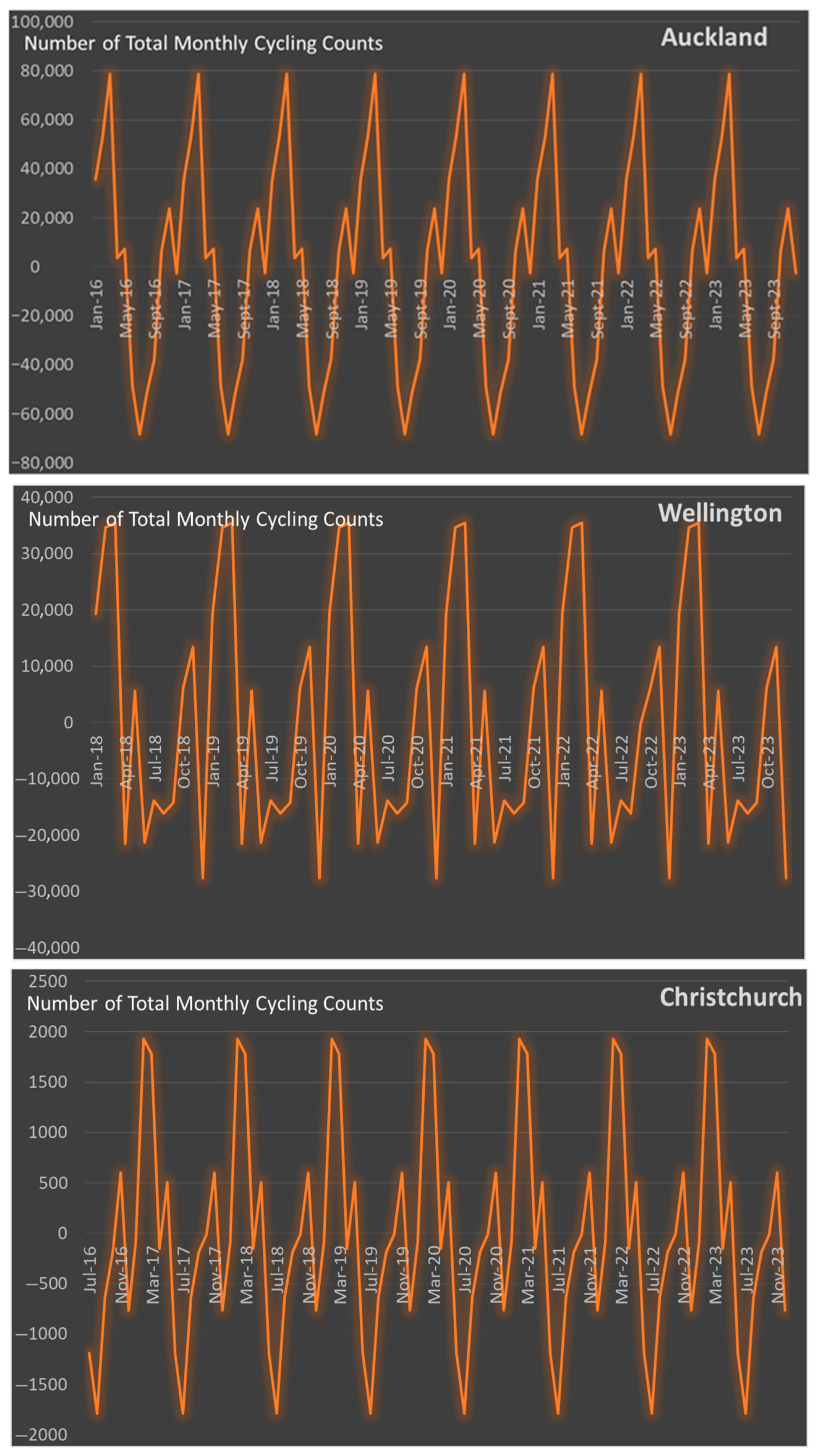
The total monthly cycling counts are presented in a time series format for each city in Figure 2. The data reveals notable heterogeneity in absolute numbers, trends, and cycling patterns across the three cities. This variability could be due to differences in city infrastructure, population density, geography, climate, or cultural factors that influence cycling habits.
Basic descriptive statistics are also provided, indicating that the computed p-value exceeds the significance level of α = 0.05. Consequently, we cannot reject the null hypothesis (H0), suggesting that the cycling numbers follow a normal distribution. The normal distribution implies that the cycling numbers are generally predictable and stable, with a regular pattern where extreme highs and lows are rare. This consistency might reflect steady cycling behavior across different times, such as predictable peak commuting hours or seasonal patterns.
A central assumption (following the results of the normal distribution) of this study is that most cycling activity is work-related, particularly commuting to and from the workplace. This hypothesis can be further evaluated by analyzing the dataset to identify relevant patterns. For example, cycling counts are expected to decline in June/July and December, coinciding with school holidays and traditional business closures. The data in Table 1 supports this assumption since both total and median cycling counts across all cities are lower during these months compared to other periods. Further evidence for this work-related cycling pattern is provided through the decomposition of each city’s monthly cycling counts into time series components. This analysis, performed using the ‘stats’ package in RStudio (2024.04), reveals a marked seasonal decline in cycling activity during June/July and December, as shown in Figure 3. These findings reinforce the assumption that cycling activity is closely related to work-related commuting patterns.
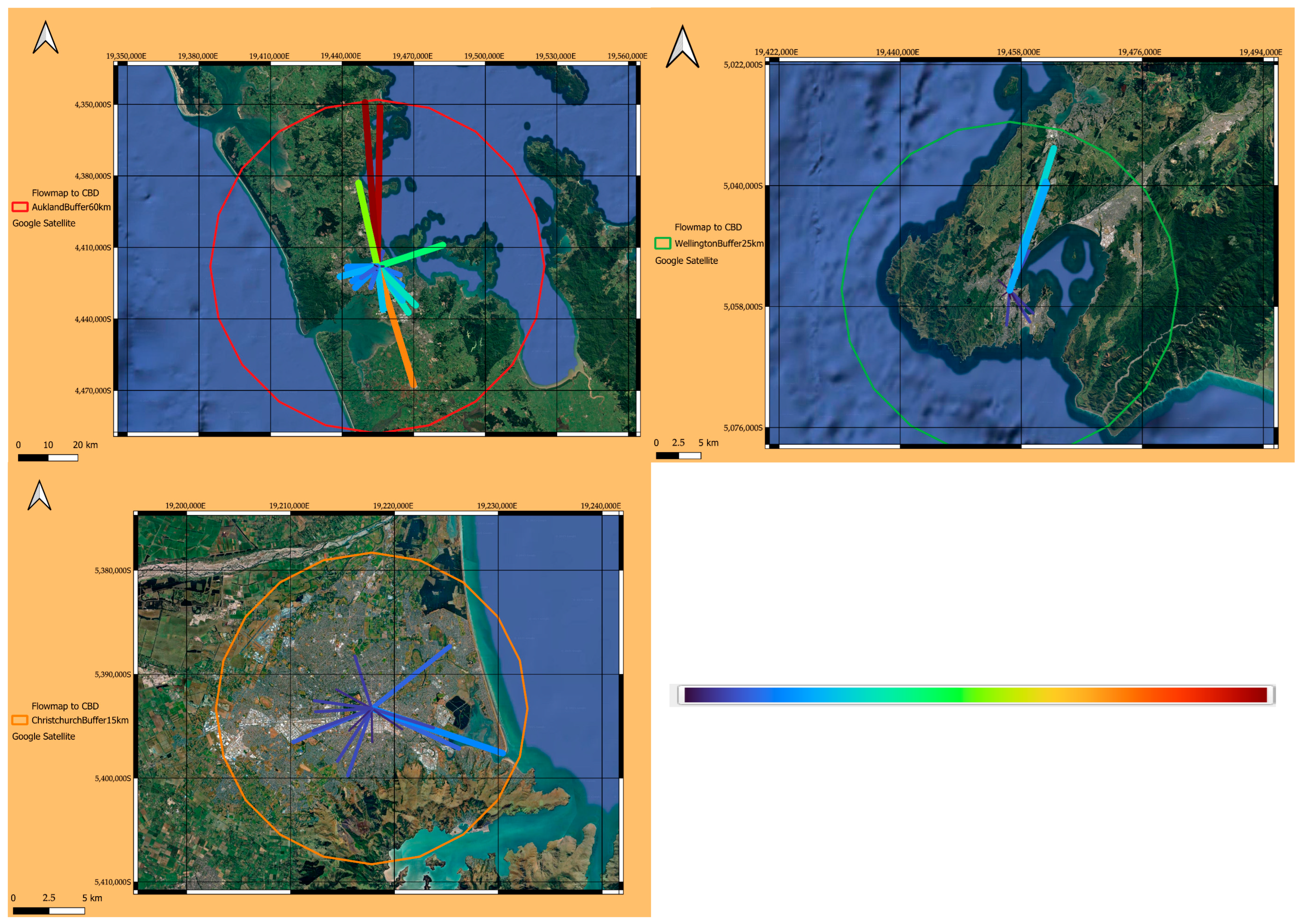
Another key assumption of this study is the existence/presence of a central workplace, which is essential for generating distance-based statistics for each cycling counter. For each city, the central workplace was assumed to be located in or around its ‘main’ or ‘historic’ central business district (CBD). This assumption enables the creation of flow maps for each city, as shown in Figure 4. These maps were developed using QGIS, with the color of each flow line representing the distance from the cycling counter to the CBD, with dark blue indicating shorter distances and dark red indicating longer distances. The red (60 km), green (25 km), and orange (15 km) circles represent the maximum buffer zones for each city, i.e., the radius equal to the farthest cycling counter from the CBD.
Additional buffer zones were established around each city’s central business district (CBD) to classify individual cycling counters based on their proximity to the CBD or assumed workplace. This approach aims to estimate cycling activity relative to distance from the workplace. A cumulative effect is anticipated, where cycling counts increase as proximity to the CBD improves, reflecting heightened cycling activity closer to the central workplace. Table 2 presents the number of cycling counters in each buffer zone. For example, there are two cycling counters within 1 km of the CBD in Auckland and Wellington, while Christchurch has only one within the same range.
The data indicates that some cities may have multiple central business districts (CBDs) or workplace hubs, as evidenced by the median cycling counts across buffer zones. For example, in Auckland, a significant concentration of cycling activity is observed between 60 km and 30 km from the presumed main CBD, suggesting the presence of a secondary business hub (Table 3). The cumulative increase in cycling counts toward the primary workplace begins at 30 km. In Wellington, the distribution of median cycling counts across buffer zones suggests that the primary CBD spans an area of at least 5 km2, with a potential secondary workplace located approximately 30 km away. Similarly, in Christchurch, the data implies the existence of either a large or secondary workplace/CBD in proximity to the main one. In all three cases, the cumulative effect of cycling counts provides compelling evidence supporting the assumptions of work-related cycling and a central workplace/CBD hub within these cities.
The identification of secondary CBDs was based on the data presented in Table 2 and Table 3, with the results visually represented in Figure 5 below. For Auckland, four decentralized secondary CBDs were identified, while Wellington and Christchurch had one and zero decentralized secondary CBDs, respectively. The establishment of these secondary CBDs significantly reduced maximum travel distances. Initially, the maximum distance recorded was 58 km. Following the addition of secondary CBDs, the maximum distance decreased to 22 km, highlighting the positive impact of decentralization on improving accessibility and reducing travel demands.
The assumption that cycling activity is work-related will be further examined using the geographically weighted regression (GWR) method to explore spatial variations and their influence on cycling patterns. Furthermore, the second assumption—regarding the presence of a central workplace—will be broadened to incorporate secondary CBDs, as suggested by the findings presented in the analysis.
Establishing an inverse relationship between distance and cycle counts will serve as crucial evidence to support the relevance and validity of these assumptions. Such a relationship would strengthen the argument that proximity plays a significant role in cycling activity, particularly within the context of work-related commutes. This approach aims to provide a more comprehensive understanding of the spatial dynamics that influence cycling behaviors.

3.2. Methodology

The study used high-quality, reliable spatially and temporally distributed cycling data across the three main urban centers of New Zealand. The study employed GWR, which extends the traditional OLS regression method by introducing a more sophisticated approach that accounts for spatial variability in relationships between independent and dependent variables. As highlighted by Lu et al. [60], GWR is a nonstationary technique that models spatially varying relationships, allowing these relationships to change across different locations; for example, the mean values vary by location. This method is grounded in Tobler’s first law of geography, which posits that “everything is related to everything else, but near things are more related than distant things” [61].
Páez and Wheeler [62] propose that GWR operates on the fundamental yet powerful principle of estimating local models using subsets of observations centered around a focal point. Since its introduction, GWR has quickly gained widespread attention in geography and related disciplines due to its ability to explore non-stationary relationships in regression analysis. The underlying concepts have also been adapted to derive local descriptive statistics and extend to other models, such as Poisson regression and probit. This method has been crucial in revealing the presence of potentially complex spatial relationships.
GWR allows for local parameters to be estimated [63] and investigates the existence of spatial non-stationarity in the relationships between a phenomenon and its determinants [64]. The general GWR equation is defined as
γ1μ = β0iμ + β1iμx1i + β2iμx2i + … + βmiμxmi
where the dependent variable “γ” at a location (µ) is regressed on a set (m) of independent variables (x) at the same location. “β” describes a relationship around the location (µ), and it is specific to that location. GWR constructs a separate equation for every spatial unit (i) of the area being studied, incorporating the dependent and explanatory variables [65].
As demonstrated in Equation (1), the fundamental concept of GWR is to investigate how the relationship between a dependent variable (Y) and one or more independent variables (X) may vary across different geographic locations, i.e., the spatial element. Unlike traditional regression models that assume a uniform relationship across the entire study area, GWR seeks to identify spatial variations. It accomplishes this by moving a search window sequentially across the dataset, analyzing one point at a time. At each point, the search window captures the surrounding data points within its radius. A regression model is then applied to this localized subset, with greater weight assigned to points closer to the focal point. Consequently, for a dataset with n observations, GWR will fit n localized regression models, allowing the examination of spatial variability in the relationships [64].
At a practical level, GWR integrates the dependent and explanatory variables of features located within the bandwidth of each target feature. The bandwidth determines the extent of the spatial neighborhood considered when fitting the local regression models. The optimal bandwidth is critical because it affects the model’s sensitivity to spatial variation. The shape and size of this bandwidth are determined by user-defined parameters, including the kernel type, Bandwidth method, distance, and number of neighbors. Therefore, when using the RStudio software program, the initial step involves estimating the appropriate bandwidth [66].

4. Results

To ensure the accuracy and robustness of the geographically weighted regression (GWR) results, the analysis was conducted in both RStudio (using the GWmodel package) and QGIS 3.40, allowing for cross-platform validation and consistency checks.
The mean and median cycle count and distance values for each of the 86 cycling counters across the three cities were log-transformed to normalize skewed distributions. For the spatial weighting, an adaptive kernel approach was employed to account for variation in counter density across space. A Gaussian kernel function was used to assign weights based on proximity.
An adaptive kernel type was selected for the GWR analysis to account for the uneven spatial distribution of cycling counters across the study area. Unlike a fixed kernel, which uses a constant bandwidth (i.e., the same distance) for all locations, an adaptive kernel adjusts the bandwidth locally to ensure a consistent number of observations are included in each local regression.
By using an adaptive kernel, the model dynamically expands the bandwidth in areas with fewer data points and contracts it in densely sampled areas, thereby improving the local fit and reducing bias. This ensures that each regression point maintains a stable level of statistical reliability while preserving spatial sensitivity. The adaptive kernel was implemented with a Gaussian weighting function, where the influence of neighboring observations decreases smoothly with increasing distance from the focal point. This method enhances the model’s ability to detect spatial heterogeneity in the relationship between cycling activity and the explanatory variables.
Bandwidth selection—a critical step in GWR—was conducted using cross-validation (CV) to minimize the residual sum of squares (RSS), ensuring the model’s goodness-of-fit while avoiding overfitting. The CV procedure evaluated a range of bandwidths to identify the optimal value that balanced local detail with model stability.
In addition, a sensitivity analysis was performed to assess the robustness of the local coefficients to bandwidth choice. Models were re-run using a range of nearest-neighbor bandwidths (e.g., 50, 75, and 100 neighbors), and key coefficient estimates remained largely consistent across scenarios. These results indicate that the model outputs are not unduly sensitive to the specific bandwidth parameter selected. Figure 5 presents the GWR-derived distance coefficients, based on the optimal bandwidth determined through this process.
All estimated coefficients are negative, ranging from −0.306 to −0.285 (as indicated in the legend of Figure 6), indicating that the relationship between distance and cycling count varies spatially. These variations in coefficients likely reflect local factors such as the presence of secondary workplaces or central business districts (CBDs), cycling infrastructure, and topographic differences.
Estimating the distance coefficients in RStudio, based on the specified parameters, yields the following results. The bandwidth is set to capture approximately 18 of the 86 data points at each location. The intercept values show spatial variation, ranging from 6.4 to 9.56, with a median of 9.25. In contrast, the global intercept of a standard OLS model is estimated at 8.69. Distance coefficients range from −0.72 to 0.47, indicating a relatively large variation in the relationship between distance and cycle count between locations. The global OLS coefficient is −0.54, representing the overall relationship between distance and cycling count if spatial variation was not considered.
The narrow range of distance coefficients derived through QGIS implies that the relationship between distance and cycling counts is spatially stable, with less variation across the areas analyzed. On the other hand, the broader range derived through RStudio, which includes both negative and positive coefficients, suggests significant spatial variability in the relationship. The negative coefficients in both analyses reinforce the assumption that an increase in distance reduces cycling activity. However, the R results suggest additional spatial complexity that may not be captured in the QGIS analysis. This is probably due to methodological differences.
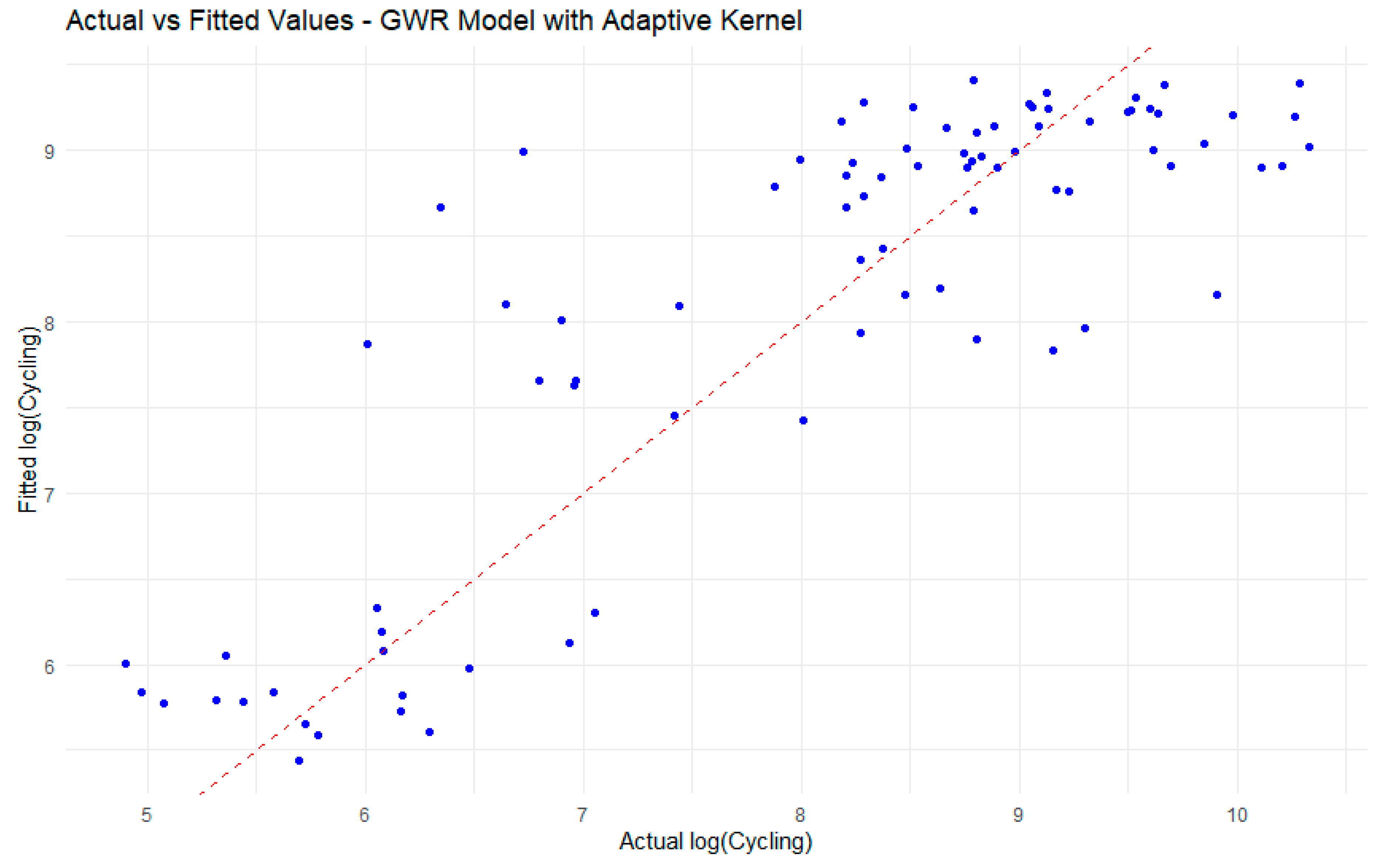
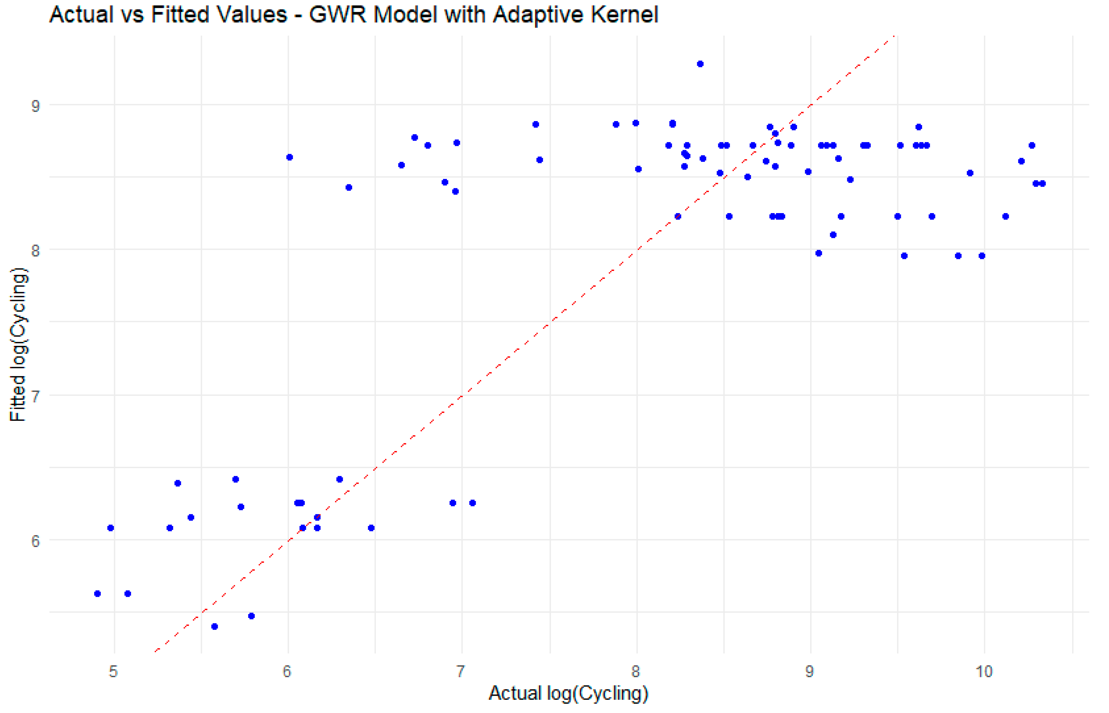
When plotting the observed versus fitted log median cycling values (Figure 7), the model demonstrates a quasi-global R2 of 73.44%, which means that approximately 73.44% of the variance in the mean cycling count is explained by the model, indicating a strong overall fit. Despite the overall strong fit, the deviations from the 45-degree line highlight areas where the model under- or overpredicts cycling counts. The observed variation in the model probably stems from local factors, as previously suggested.
The literature [14,40] suggests that weather, particularly precipitation, significantly impacts cycling volumes. Following the distance-based assessment, the effect of precipitation on cycling volumes will be examined using the GWR method. Establishing an inverse relationship between precipitation and cycling counts would provide further evidence of the connection between weather conditions and cycling activity.
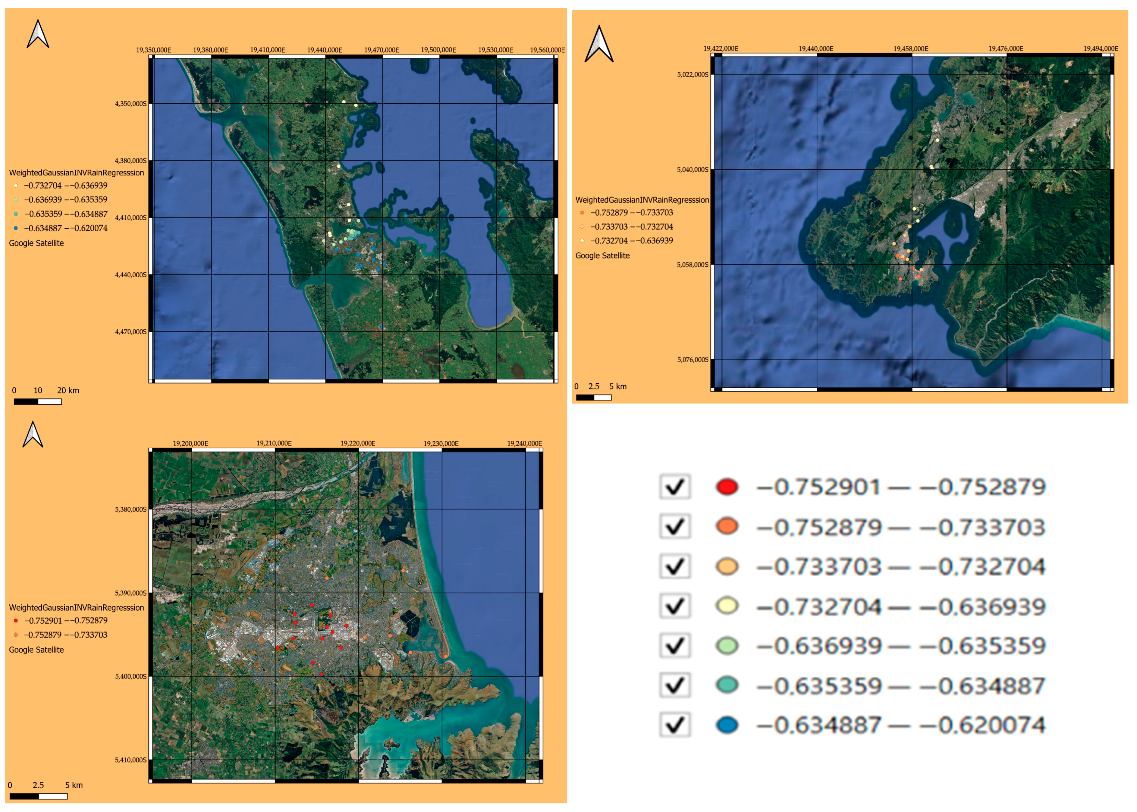
To enhance accuracy and robustness, the GWR method will be implemented in both RStudio and QGIS, facilitating cross-validation between platforms. For the analysis, the mean and median cycling counts and precipitation values for each of the 86 cycling counters across the three cities were log-transformed to normalize the data. In QGIS, the analysis parameters, including an adaptive kernel type and a Gaussian bandwidth search method, generated the precipitation coefficients shown in Figure 8. The estimated log coefficients, which are uniformly negative and range from −0.753 to −0.62 (as indicated in the legend of Figure 8), demonstrate a spatially variable relationship between precipitation and cycling counts. These spatial variations in coefficients likely reflect local influences, such as climatic and topographic differences.
Estimating the distance coefficients in RStudio, based on the specified parameters, yields the following results. The bandwidth is set to capture approximately 44 of the 86 data points at each location. The intercept values exhibit spatial variation, ranging from 24.156 to 29.815, with a median of 25.390. In contrast, the global intercept of a standard OLS model is estimated at 29.076. The log precipitation coefficients range from −99.662 to −73.620, indicating variation in the relationship between precipitation and cycling count across locations. The global OLS log coefficient is −96.461, representing the overall relationship between precipitation and cycling count if spatial variation was not considered.
The coefficients for log rain values derived from the geographically weighted regression model vary significantly between QGIS and R. The range of coefficients for the log rain variable in QGIS is between −0.753 and −0.62, while the range for the log rain coefficients in R spans from −99.662 to −73.620, which is significantly wider than the QGIS results. This disparity in coefficients is the result of the different modeling results given the software and its associated parameters, which could be influenced by how each environment handles spatial autocorrelation, bandwidth selection, or data scaling. The negative relationship between rainfall and cycling counts is clear, but the strength and consistency of this relationship need further analysis.
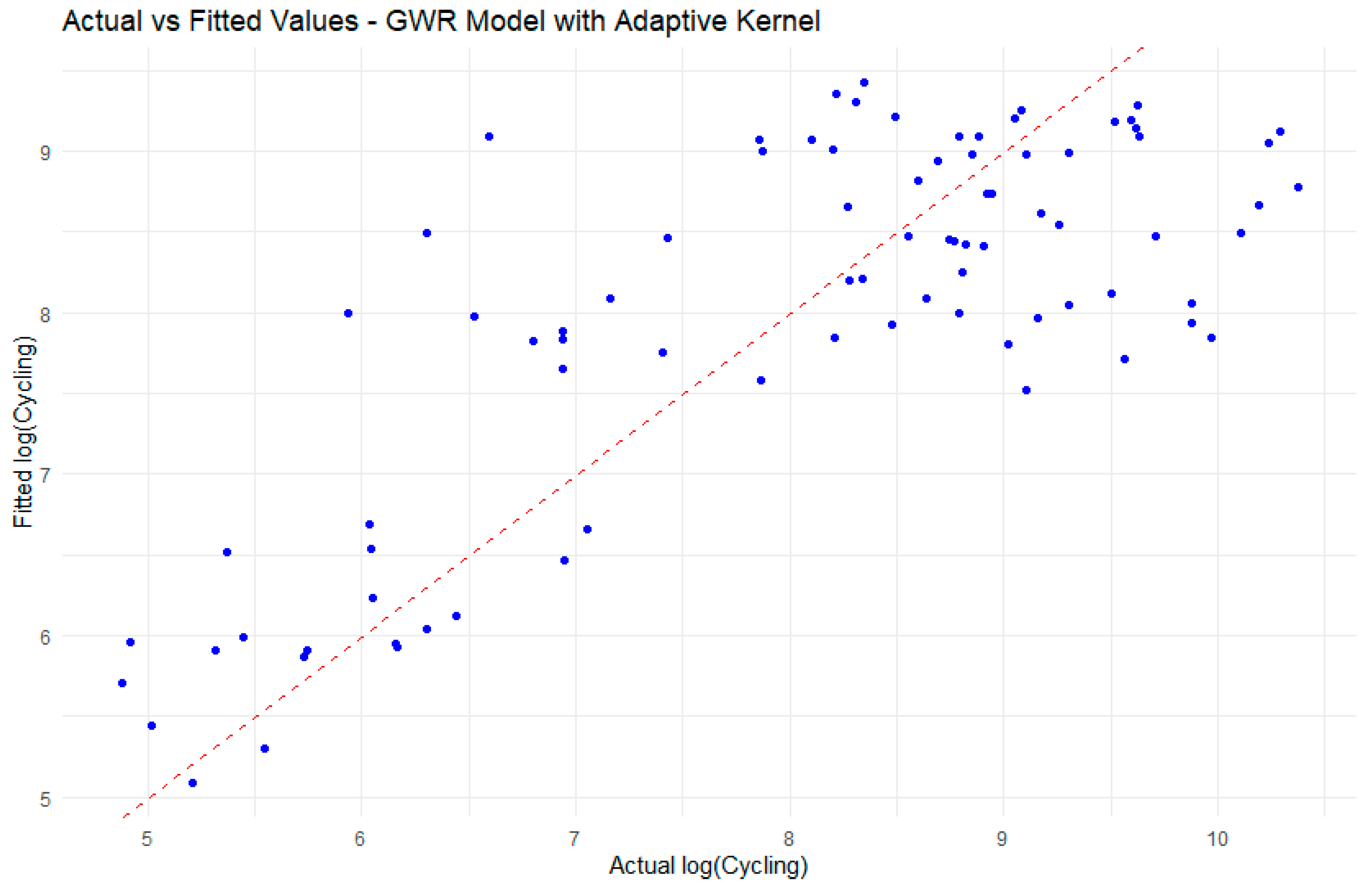
When plotting the observed versus fitted log mean cycling values (Figure 9), the model demonstrates a quasi-global R2 of 54.10%, which means that approximately 54.10% of the variance in the mean cycling count is explained by the model, indicating a moderate overall fit. The observed variation in the model likely stems from local factors such as climatic and topographic differences, as previously suggested.
In this analysis, a multiple geographically weighted regression model was developed to examine the combined influence of distance and precipitation on the response variable. The results, summarized in Table 4 and illustrated in Figure 10, provide insights into the spatial variability of these relationships. The model uses a bandwidth calibrated to include approximately 44 of the 86 data points at each location, ensuring an optimal balance between local specificity and broader spatial trends.
The GWR coefficients—intercept (X.Intercept), log-transformed distance (lndistance), and log-transformed precipitation (inrlnrain)—demonstrate spatial heterogeneity across the study area. Table 4 summarizes these estimates, while global coefficients from an OLS model are provided for comparison.
The intercept values exhibit significant spatial variation, ranging from 16.37 to 29.91, with a median value of 21.16. This variability suggests that the baseline levels of the response variable are not uniform across the study area, possibly influenced by unobserved spatial factors or the interaction of distance and precipitation with local conditions. The global intercept from the OLS model is 29.40, which falls near the upper quartile of the GWR-derived intercepts. This highlights the added value of GWR in capturing local deviations that are masked by global models. The coefficients for log-transformed distance vary narrowly between −0.573 and −0.472, with a median of −0.559. These values suggest a consistent negative relationship between distance and the response variable, with greater distances generally associated with lower outcomes. The global OLS coefficient (−0.500) lies near the midpoint of the GWR range, indicating that while distance effects are relatively stable, local variability can refine the model’s predictive accuracy.
The coefficients for log-transformed precipitation (inrlnrain) demonstrate more substantial spatial variability, ranging from −97.63 to −33.47, with a median of −56.21. This wide range indicates that precipitation’s influence on the response variable is highly localized, likely reflecting differences in how precipitation interacts with regional environmental or socioeconomic factors. The global coefficient (−95.23) is close to the lower bound of the GWR range, suggesting that, in some areas, the effect of precipitation is less pronounced than implied by the global model.
The spatial heterogeneity of the GWR coefficients underscores the importance of accounting for local variations in distance and precipitation when modeling the response variable. Unlike OLS, which assumes uniform effects across the entire study area, GWR reveals nuanced spatial patterns that can inform targeted interventions or policies.
When plotting the observed versus fitted log median cycling values (Figure 10), the model shows a quasi-global R2 of 60.19%, which means that approximately 60% of the variance in the mean cycling count is explained by the model, indicating a relatively strong overall fit. Despite the overall strong fit, the deviations from the 45-degree line highlight areas where the model under- or overpredicts cycling counts. The observed variation in the model probably stems from local factors, as previously suggested.

5. Discussion

Two critical assumptions regarding cycling volumes were evaluated in three major cities in New Zealand. The analysis first applied a single-equation GWR model to assess localized distance and precipitation relationships with cycling volumes. Subsequently, the analysis advanced to multiple equation models to capture the interaction of multiple factors and enhance the robustness of the findings. This methodological approach ensured a comprehensive understanding of the spatial variability and contextual factors influencing the volumes of bicycles in three diverse urban environments.

5.1. Spatial Variability Mechanisms

The three New Zealand cities that were used for this analysis are individually unique—in their urban design, transport network, location, topography, and micro-climate, to name a few—which is broadly captured through spatial variability. These unique features influence the use of cycling for each city, as evident from the GWR models. Ignoring the spatial uniqueness through the application of the OLS shows that overall cycling use decreases as distance and precipitation increase, with the log(distance) coefficient estimated at −0.43 and the log(precipitation) coefficient estimated at −99.42. This is a general finding and supported throughout the literature when ignoring spatial variability. The GWR results reveal there are location-specific factors shaping cycling volumes for each of these cities, with substantial variations in the coefficients for both distance and precipitation across different locations. This method provides improved statistical interpretation compared to OLS regression, highlighting the differing spatial relationships between cycling volumes and distance to central business districts. For single-equation GWR models, the coefficient for log(distance) ranged from −0.72 to 0.47. This indicates that, in some locations, increased distance significantly deters cycling volumes (e.g., a 1% increase in distance leads to a 0.72% decrease in cycling volumes), while in others, a positive relationship is observed, potentially reflecting unique urban design, infrastructure, topography, or sociodemographic factors that make cycling over longer distances more feasible or attractive.
For example, in areas with better rain-resistant cycling infrastructure or higher levels of cycling culture, especially for utilitarian use, the impact of precipitation may be less severe, a result supported in the literature [67].
In contrast, the multiple-equation GWR models showed narrower ranges for the coefficients, reflecting the incorporation of additional contextual variables that account for some of the variability observed in the single-equation models. Specifically, the log(distance) coefficients in the multiple-equation models ranged from −0.45 to −0.43, indicating a consistently negative relationship between distance and cycling volumes across locations. The log(precipitation) coefficients ranged from −101.23 to −89.03, further confirming the strong and uniform deterring effect of precipitation on cycling volumes. The spatial model reveals that the relationship between distance and cycle count is not uniform across space, with some areas showing a negative effect between distance and cycling, while others are positive. The global OLS model hides these complexities, which are shown in the GWR model.

5.2. Implications

Closer examination of the results reveals compelling location-specific patterns. The coefficients for logarithmic distance and log precipitation, derived using a GWR analysis performed in QGIS for the 86 cycling counters across three cities, are presented in Table 4. The findings provide valuable behavioral and contextual insights into utilitarian cycling activity and the factors that influence the link between the periphery and areas of high employment. The practical implications for urban cycleway planning reveal the following:
Across all cities, cycling demonstrates lower sensitivity to changes in distance compared to variations in weather conditions. Adverse weather conditions, such as rainfall, appear to have a more significant impact on cycling behavior than the physical distance of cycling routes. This suggests that to promote cycling, cities should prioritize addressing weather-related barriers. Strategies could include investing in weather-resistant cycling infrastructure, such as covered bike lanes or rain shelters, and offering real-time weather updates to help cyclists plan their trips.
At the city level, Auckland displays significantly lower distance sensitivity compared with the other two cities. Cyclists in Auckland are more likely to continue cycling as distance increases. This finding is unexpected, especially given that Wellington’s topography is similar to that of Auckland with its hills, while Christchurch has a predominantly flat terrain. This variation could be attributed to Auckland’s specific characteristics, such as its topography, urban design, or availability of alternative transportation modes. Auckland has well-developed secondary CBDs, whereas Christchurch and Wellington have one central business district (CBD). This suggests that utilitarian cycling behavior is affected by the urban framework and location of the primary and secondary central business districts. Addressing these unique factors by improving cycling route infrastructure to secondary employment nodes, rather than only the main node, could mitigate the impact of distance on cycling behavior in each city. Decentralized employment nodes reduce the distance to job opportunities, supporting the transition from motorized transport to cycling as an alternative. Observing the GWR results for the decentralized nodes in Auckland reveals that spatial variation in cycling volumes remains strong even when distance increases away from the main CBD.
Within each city, there is limited variance among individual cycling counters in terms of distance sensitivity. This consistency suggests that distance-related cycling patterns are relatively uniform within each urban area. Consequently, city-wide approaches to improving cycling infrastructure could yield broad benefits without the need for highly localized interventions targeting distance-related barriers.
In contrast to the distance variable, the precipitation variable remains negative with the use of the GWR method, highlighting and supporting existing research that demonstrates that climate and topographical features negatively influence utilitarian cycling volumes. With this in mind, the results from the GWR method show spatial variation, while not all localities share the same magnitude of this negative relationship.
At the city level, the sensitivity to precipitation is higher in Christchurch (−0.75) compared with Auckland (−0.63) and Wellington (−0.73), even though Christchurch has lower annual rainfall (675 mm) compared to Auckland (1090 mm) and Wellington (1346 mm). These intercity differences in weather sensitivity could be related to factors such as the availability of weather-resilient infrastructure, cultural attitudes towards cycling under adverse conditions, or the level of public awareness of the benefits of cycling regardless of weather. Wellington and Christchurch, in contrast, show more consistent weather sensitivity, indicating a more stable relationship between precipitation and cycling behavior.

6. Conclusions

The complexity of cities increases as they grow, requiring a response within the urban land continuum as choices are made that relate to the use of existing and new land for economic development. Promoting cycling as an alternative mode of transport is argued to be a key contributor to achieving sustainability goals for many cities. As a result, significant amounts of investment are poured into infrastructure that encourages shifting behavior for consumers, encouraging utilitarian bicycle use in addition to recreational use. Due to its continuous nature, the cycling data applied in this study represents one of the longest time series panels used in the evaluation of cycling volumes in relation to distance and precipitation.
The findings align with theoretical expectations: increased distance and higher precipitation levels are well-known deterrents to cycling activity. The logarithmic transformation of the variables allows for a proportional interpretation of these effects, enhancing the model’s ability to capture elasticities and the relative magnitude of the relationships across different contexts. The GWR approach allows an assessment of the individual spatial relevance of cycling volumes at different distances to main employment areas. This provides improved statistical interpretation compared to OLS regression, which only provides a global coefficient between cycling volumes and distance and hides the complexities.
The findings of the study contribute to urban science by demonstrating the interplay between distance and cycling as a key determinant in volumes of use. It supports the finding of Broach et al. [68] that cyclists are sensitive to distance; however, this work adds to the finding that city size is a moderating factor, as the distance sensitivity for Wellington, Christchurch, and Ackland was different. Secondly, cycling use is sensitive to weather conditions [2]. In addition, micro-climate and daily weather changes possibly influence the utilization of cycling infrastructure, with cycling numbers more responsive in Auckland than Christchurch as a result of weather.
These findings underscore the complexity of spatial interactions and emphasize the need for localized interventions when planning to promote cycling. The variability in coefficients across locations suggests that, while distance and precipitation have general effects, local factors such as infrastructure quality, topography, weather adaptation measures, and cultural attitudes toward cycling play a critical role in modulating these relationships. We acknowledge that all automated counting systems have limitations, and future work could explore validation or calibration techniques where necessary. In addition, the impacts of precipitation on cycling activity can vary depending on accompanying factors like wind and temperature. Future analysis could incorporate these additional variables to better isolate the effects of specific weather conditions on cycling behavior.

Author Contributions

Conceptualization, D.D. and C.E.C.; methodology, C.E.C.; software, C.E.C.; validation, D.D. and C.E.C.; formal analysis, D.D. and C.E.C.; investigation, D.D. and C.E.C.; resources, D.D. and C.E.C.; data curation, D.D. and C.E.C.; writing—original draft preparation, D.D.; C.E.C. and E.K.; writing—review and editing, D.D., C.E.C. and E.K.; visualization, C.E.C.; project administration, D.D. All authors have read and agreed to the published version of the manuscript.

Funding

APC funding for this article was provided for by the North-West University, South Africa.

Institutional Review Board Statement

Not applicable.

Informed Consent Statement

Not applicable.

Data Availability Statement

The original data presented in the study are openly available in Data@lincoln at https://doi.org/10.25400/lincolnuninz.29378948.v1.

Conflicts of Interest

The authors declare no conflict of interest.

References

  1. Oviedo, D.; Sabogal-Cardona, O. Arguments for Cycling as a Mechanism for Sustainable Modal Shifts in Bogotá. J. Transp. Geogr. 2022, 99, 103291. [Google Scholar] [CrossRef]
  2. Nankervis, M. The Effect of Weather and Climate on Bicycle Commuting. Transp. Res. Part A Policy Pract. 1999, 33, 417–431. [Google Scholar] [CrossRef]
  3. An, R.; Zahnow, R.; Pojani, D.; Corcoran, J. Weather and Cycling in New York: The Case of Citibike. J. Transp. Geogr. 2019, 77, 97–112. [Google Scholar] [CrossRef]
  4. Schneider, F.; Jensen, A.F.; Daamen, W.; Hoogendoorn, S. Empirical Analysis of Cycling Distances in Three of Europe’s Most Bicycle-Friendly Regions within an Accessibility Framework. Int. J. Sustain. Transp. 2023, 17, 775–789. [Google Scholar] [CrossRef]
  5. Wardman, M.; Tight, M.; Page, M. Factors Influencing the Propensity to Cycle to Work. Transp. Res. Part A Policy Pract. 2007, 41, 339–350. [Google Scholar] [CrossRef]
  6. Tyndall, J. Cycling Mode Choice amongst US Commuters: The Role of Climate and Topography. Urban Stud. 2022, 59, 97–119. [Google Scholar] [CrossRef]
  7. Howard, C.; Burns, E.K. Cycling to Work in Phoenix: Route Choice, Travel Behavior, and Commuter Characteristics. Transp. Res. Rec. J. Transp. Res. Board 2001, 1773, 39–46. [Google Scholar] [CrossRef]
  8. Goodman, A.; Sahlqvist, S.; Ogilvie, D. Who Uses New Walking and Cycling Infrastructure and How? Longitudinal Results from the UK IConnect Study. Prev. Med. 2013, 57, 518–524. [Google Scholar] [CrossRef]
  9. Sun, Y.; Mobasheri, A.; Hu, X.; Wang, W. Investigating Impacts of Environmental Factors on the Cycling Behavior of Bicycle-Sharing Users. Sustainability 2017, 9, 1060. [Google Scholar] [CrossRef]
  10. Wilson, O.; Vairo, N.; Bopp, M.; Sims, D.; Dutt, K.; Pinkos, B. Best Practices for Promoting Cycling amongst University Students and Employees. J. Transp. Health 2018, 9, 234–243. [Google Scholar] [CrossRef]
  11. Pucher, J.; Buehler, R. Safer Cycling Through Improved Infrastructure. Am. J. Public Health 2016, 106, 2089–2091. [Google Scholar] [CrossRef] [PubMed]
  12. Çiriş, S.; Akay, M.; Tümer, E. Investigating the Influence of Spatial Characteristics on Cycling Volume: A Multi-Scale Geographic Weighted Regression Approach. Transp. Res. Interdiscip. Perspect. 2024, 26, 101160. [Google Scholar] [CrossRef]
  13. Munira, S.; Sener, I.N. A Geographically Weighted Regression Model to Examine the Spatial Variation of the Socioeconomic and Land-Use Factors Associated with Strava Bike Activity in Austin, Texas. J. Transp. Geogr. 2020, 88, 102865. [Google Scholar] [CrossRef]
  14. Schmiedeskamp, P.; Zhao, W. Estimating Daily Bicycle Counts in Seattle, Washington, from Seasonal and Weather Factors. Transp. Res. Rec. J. Transp. Res. Board 2016, 2593, 94–102. [Google Scholar] [CrossRef]
  15. Miranda-Moreno, L.F.; Nosal, T.; Schneider, R.J.; Proulx, F. Classification of Bicycle Traffic Patterns in Five North American Cities. Transp. Res. Rec. J. Transp. Res. Board 2013, 2339, 68–79. [Google Scholar] [CrossRef]
  16. Chen, P.; Zhou, J.; Sun, F. Built Environment Determinants of Bicycle Volume: A Longitudinal Analysis. J. Transp. Land Use 2017, 10, 655–674. [Google Scholar] [CrossRef]
  17. Lv, H.; Li, H.; Sze, N.N.; Zhang, Z.; Ren, G.; Zhang, Y. Analysis of Factors Influencing Cycling Count: A Micro-Level Study Using Road Segment Count Data in London. Int. J. Sustain. Transp. 2023, 17, 1113–1128. [Google Scholar] [CrossRef]
  18. Jean-Louis, G.; Eckhardt, M.; Podschun, S.; Mahnkopf, J.; Venohr, M. Estimating Daily Bicycle Counts with Strava Data in Rural and Urban Locations. Travel Behav. Soc. 2024, 34, 100694. [Google Scholar] [CrossRef]
  19. NZ Transport Agency Waka Kotahi Urban Cycleways Programme. Available online: https://www.nzta.govt.nz/walking-cycling-and-public-transport/cycling/investing-in-cycling/urban-cycleways-programme?start=0 (accessed on 14 August 2024).
  20. Ministry for the Environment. Te Hau Mārohi Ki Anamata: Towards a Productive, Sustainable and Inclusive Economy: Aotearoa New Zealand’s First Emissions Reduction Plan; Ministry for the Environment Manatu Mo Te Taiao: Wellington, New Zealand, 2022; ISBN 9781991025265.
  21. Keall, M.D.; Shaw, C.; Chapman, R.; Howden-Chapman, P. Reductions in Carbon Dioxide Emissions from an Intervention to Promote Cycling and Walking: A Case Study from New Zealand. Transp. Res. D Transp. Environ. 2018, 65, 687–696. [Google Scholar] [CrossRef]
  22. Aldy, J.E.; Pizer, W.A.; Akimoto, K. Climate Policy Comparing Emissions Mitigation Efforts across Countries Comparing Emissions Mitigation Efforts across Countries. Cent. Glob. Dev. Work. Pap. 2016, 17, 501–515. [Google Scholar] [CrossRef]
  23. Bhowmick, D.; Saberi, M.; Stevenson, M.; Thompson, J.; Winters, M.; Nelson, T.; Leao, S.Z.; Seneviratne, S.; Pettit, C.; Vu, H.L.; et al. A Systematic Scoping Review of Methods for Estimating Link-Level Bicycling Volumes. Transp. Rev. 2023, 43, 622–651. [Google Scholar] [CrossRef]
  24. Zare, P.; Leao, S.; Gudes, O.; Pettit, C. A Simple Agent-Based Model for Planning for Bicycling: Simulation of Bicyclists’ Movements in Urban Environments. Comput. Environ. Urban Syst. 2024, 108, 102059. [Google Scholar] [CrossRef]
  25. Yang, Y.; Wu, X.; Zhou, P.; Gou, Z.; Lu, Y. Towards a Cycling-Friendly City: An Updated Review of the Associations between Built Environment and Cycling Behaviors (2007–2017). J. Transp. Health 2019, 14, 100613. [Google Scholar] [CrossRef]
  26. Moustaka, V.; Vakali, A.; Anthopoulos, L.G. A Systematic Review for Smart City Data Analytics. ACM Comput. Surv. 2019, 51, 1–41. [Google Scholar] [CrossRef]
  27. Borsekova, K.; Vanova, A.; Vitalisova, K. The Power of Communities in Smart Urban Development. Procedia Soc. Behav. Sci. 2016, 223, 51–57. [Google Scholar] [CrossRef]
  28. Kandt, J.; Batty, M. Smart Cities, Big Data and Urban Policy: Towards Urban Analytics for the Long Run. Cities 2021, 109, 102992. [Google Scholar] [CrossRef]
  29. Dyason, D.; Fieger, P.; Rice, J. Greened Shopping Spaces and Pedestrian Shopping Interactions: The Case of Christchurch. Int. J. Tour. Cities 2024, 10, 1247–1265. [Google Scholar] [CrossRef]
  30. Yigitcanlar, T. Smart Cities: An Effective Urban Development and Management Model? Aust. Plan. 2015, 52, 27–34. [Google Scholar] [CrossRef]
  31. Hou, Q.; Li, W.; Zhang, X.; Fang, Y.; Duan, Y.; Zhang, L.; Liu, W. Intelligent Urban Planning on Smart City Blocks Based on Bicycle Travel Data Sensing. Comput. Commun. 2020, 153, 26–33. [Google Scholar] [CrossRef]
  32. Pucher, J.; Buehler, R. Making Cycling Irresistible: Lessons from The Netherlands, Denmark and Germany. Transp. Rev. 2008, 28, 495–528. [Google Scholar] [CrossRef]
  33. Lopes, M.; Mélice Dias, A.; Silva, C. The Impact of Urban Features in Cycling Potential—A Tale of Portuguese Cities. J. Transp. Geogr. 2021, 95, 103149. [Google Scholar] [CrossRef]
  34. Goel, R.; Goodman, A.; Aldred, R.; Nakamura, R.; Martin, L.; Garcia, T.; Zapata-Diomedi, B.; Herick De Sa, T.; Tiwari, G.; De Nazelle, A.; et al. Cycling Behaviour in 17 Countries across 6 Continents: Levels of Cycling, Who Cycles, for What Purpose, and How Far? Transp. Rev. 2021, 42, 58–81. [Google Scholar] [CrossRef]
  35. Hull, A.; O’Holleran, C. Bicycle Infrastructure: Can Good Design Encourage Cycling? Urban Plan. Transp. Res. 2014, 2, 369–406. [Google Scholar] [CrossRef]
  36. Pucher, J.; Buehler, R. Cycling towards a More Sustainable Transport Future. Transp. Rev. 2017, 37, 689–694. [Google Scholar] [CrossRef]
  37. Carvajal, G.A.; Sarmiento, O.L.; Medaglia, A.L.; Cabrales, S.; Rodríguez, D.A.; Quistberg, D.A.; López, S. Bicycle Safety in Bogotá: A Seven-Year Analysis of Bicyclists’ Collisions and Fatalities. Accid. Anal. Prev. 2020, 144, 105596. [Google Scholar] [CrossRef]
  38. Gössling, S.; McRae, S. Subjectively Safe Cycling Infrastructure: New Insights for Urban Designs. J. Transp. Geogr. 2022, 101, 103340. [Google Scholar] [CrossRef]
  39. Pasha, M.; Rifaat, S.; Tay, R.; De Barros, A. Urban Design and Planning Influences on the Share of Trips Taken by Cycling. J. Urban Des. 2016, 21, 471–480. [Google Scholar] [CrossRef]
  40. Nosal, T.; Miranda-Moreno, L.F. The Effect of Weather on the Use of North American Bicycle Facilities: A Multi-City Analysis Using Automatic Counts. Transp. Res. Part A Policy Pract. 2014, 66, 213–225. [Google Scholar] [CrossRef]
  41. Levy, N.; Golani, C.; Ben-Elia, E. An Exploratory Study of Spatial Patterns of Cycling in Tel Aviv Using Passively Generated Bike-Sharing Data. J. Transp. Geogr. 2019, 76, 325–334. [Google Scholar] [CrossRef]
  42. Lee, K.; Sener, I.N. Emerging Data for Pedestrian and Bicycle Monitoring: Sources and Applications. Transp. Res. Interdiscip. Perspect. 2020, 4, 100095. [Google Scholar] [CrossRef]
  43. Dadashova, B.; Griffin, G.P.; Das, S.; Turner, S.; Sherman, B. Estimation of Average Annual Daily Bicycle Counts Using Crowdsourced Strava Data. Transp. Res. Rec. J. Transp. Res. Board 2020, 2674, 390–402. [Google Scholar] [CrossRef]
  44. Fishman, E.; Washington, S.; Haworth, N. Bike Share: A Synthesis of the Literature. Transp. Rev. 2013, 33, 148–165. [Google Scholar] [CrossRef]
  45. Kaltenbrunner, A.; Meza, R.; Grivolla, J.; Codina, J.; Banchs, R. Urban Cycles and Mobility Patterns: Exploring and Predicting Trends in a Bicycle-Based Public Transport System. Pervasive Mob. Comput. 2010, 6, 455–466. [Google Scholar] [CrossRef]
  46. Lathia, N.; Ahmed, S.; Capra, L. Measuring the Impact of Opening the London Shared Bicycle Scheme to Casual Users. Transp. Res. Part C Emerg. Technol. 2012, 22, 88–102. [Google Scholar] [CrossRef]
  47. Zhang, Y.; Thomas, T.; Brussel, M.; van Maarseveen, M. Exploring the Impact of Built Environment Factors on the Use of Public Bikes at Bike Stations: Case Study in Zhongshan, China. J. Transp. Geogr. 2017, 58, 59–70. [Google Scholar] [CrossRef]
  48. Tran, T.D.; Ovtracht, N.; D’Arcier, B.F. Modeling Bike Sharing System Using Built Environment Factors. Procedia CIRP 2015, 30, 293–298. [Google Scholar] [CrossRef]
  49. Singhvi, D.; Singhvi, S.; Frazier, P.I.; Henderson, S.G.; O’ Mahony, E.; Shmoys, D.B.; Woodard, D.B. Predicting Bike Usage for New York City’s Bike Sharing System. AAAI Workshop Comput. Sustain. 2015, 110–114. [Google Scholar]
  50. Lin, J.J.; Zhao, P.; Takada, K.; Li, S.; Yai, T.; Chen, C.H. Built Environment and Public Bike Usage for Metro Access: A Comparison of Neighborhoods in Beijing, Taipei, and Tokyo. Transp. Res. D Transp. Environ. 2018, 63, 209–221. [Google Scholar] [CrossRef]
  51. Kou, Z.; Cai, H. Understanding Bike Sharing Travel Patterns: An Analysis of Trip Data from Eight Cities. Phys. A Stat. Mech. Its Appl. 2019, 515, 785–797. [Google Scholar] [CrossRef]
  52. Vogel, P.; Greiser, T.; Mattfeld, D.C. Understanding Bike-Sharing Systems Using Data Mining: Exploring Activity Patterns. Procedia Soc. Behav. Sci. 2011, 20, 514–523. [Google Scholar] [CrossRef]
  53. Yang, H.; Lu, X.; Cherry, C.; Liu, X.; Li, Y. Spatial Variations in Active Mode Trip Volume at Intersections: A Local Analysis Utilizing Geographically Weighted Regression. J. Transp. Geogr. 2017, 64, 184–194. [Google Scholar] [CrossRef]
  54. Bao, J.; Shi, X.; Zhang, H. Spatial Analysis of Bikeshare Ridership with Smart Card and POI Data Using Geographically Weighted Regression Method. IEEE Access 2018, 6, 76049–76059. [Google Scholar] [CrossRef]
  55. Wei, Z.; Zhen, F.; Mo, H.; Wei, S.; Peng, D.; Zhang, Y. Travel Behaviours of Sharing Bicycles in the Central Urban Area Based on Geographically Weighted Regression: The Case of Guangzhou, China. Chin. Geogr. Sci. 2021, 31, 54–69. [Google Scholar] [CrossRef]
  56. Wellington City Council Cycle Count Data. Available online: https://www.transportprojects.org.nz/cycle-data (accessed on 3 December 2024).
  57. Christchurch City Council Cycle Counters. Available online: https://smartview.ccc.govt.nz/data/cycle-counters (accessed on 3 December 2024).
  58. Auckland Transport Monthly Cycle Monitoring. Available online: https://at.govt.nz/cycling-walking/research-monitoring/monthly-cycle-monitoring (accessed on 3 December 2024).
  59. Coetzee, C.; Dyason, D. Cycling Activity in New Zealand’s Three Largest Cities; Dataset; Lincoln University: Lincoln, New Zealand, 2025. [Google Scholar] [CrossRef]
  60. Lu, B.; Charlton, M.; Harris, P.; Fotheringham, A.S. Geographically Weighted Regression with a Non-Euclidean Distance Metric: A Case Study Using Hedonic House Price Data. Int. J. Geogr. Inf. Sci. 2014, 28, 660–681. [Google Scholar] [CrossRef]
  61. Zheng, B.; Lin, X.; Yin, D.; Qi, X. Does Tobler’s First Law of Geography Apply to Internet Attention? A Case Study of the Asian Elephant Northern Migration Event. PLoS ONE 2023, 18, e0282474. [Google Scholar] [CrossRef]
  62. Páez, A.; Wheeler, D.C. Geographically Weighted Regression. In International Encyclopedia of Human Geography; Elsevier: Amsterdam, The Netherlands, 2009; pp. 407–414. [Google Scholar]
  63. Fotheringham, A.S.; Brunsdon, C. Local Forms of Spatial Analysis. Geogr. Anal. 1999, 31, 340–358. [Google Scholar] [CrossRef]
  64. Fotheringham, A.S.; Brunsdon, C.; Charlton, M. Geographically Weighted Regression: The Analysis of Spatially Varying Relationships; John Wiley & Sons Ltd.: West Sussex, UK, 2002. [Google Scholar]
  65. Faka, A.; Kalogeropoulos, K.; Chalkias, C. Quality of Life in Athens, Greece, Using Geonformatics. In Geoinformatics for Geosciences; Elsevier: Amsterdam, The Netherlands, 2023; pp. 31–44. [Google Scholar]
  66. Mendez, C. Geographically Weighted Regression Models: A Tutorial Using the Spgwr Package in R 2020. Available online: https://rpubs.com/quarcs-lab/tutorial-gwr1 (accessed on 3 February 2025).
  67. Thomas, T.; Jaarsma, R.; Tutert, B.; Thomas, T.; Tutert, Á.B.; Tutert, B.; Jaarsma, R. Exploring Temporal Fluctuations of Daily Cycling Demand on Dutch Cycle Paths: The Influence of Weather on Cycling. Transportation 2013, 40, 1–22. [Google Scholar] [CrossRef]
  68. Broach, J.; Dill, J.; Gliebe, J. Where Do Cyclists Ride? A Route Choice Model Developed with Revealed Preference GPS Data. Transp. Res. Part A Policy Pract. 2012, 46, 1730–1740. [Google Scholar] [CrossRef]
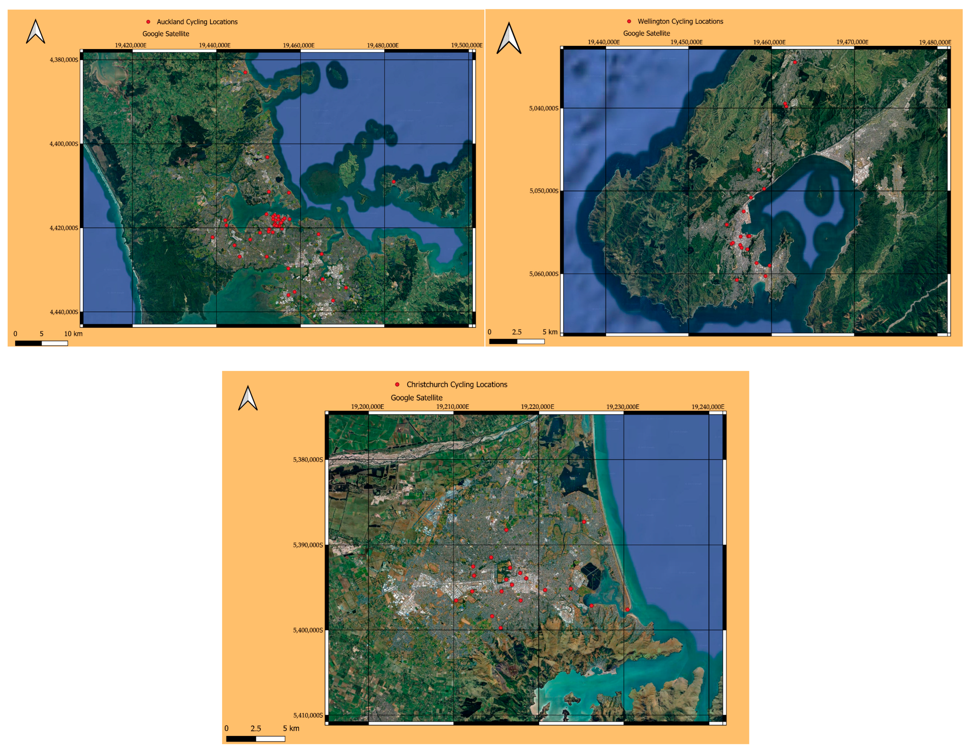
Figure 1. Location of the cycling counters per city. Source: authors’ analysis.
Smartcities 08 00133 g001
Figure 2. Cycling counter count time series and descriptive statistics per city. Source: authors’ analysis.
Smartcities 08 00133 g002aSmartcities 08 00133 g002b
Figure 3. Seasonal component of the total cycling count per city. Top image = Auckland, middle image = Wellington, and bottom image = Christchurch. Source: authors’ analysis.
Smartcities 08 00133 g003
Figure 4. Cycling counter distance flow maps. Source: authors’ analysis. Dark blue indicates shorter distances and dark red indicates longer distances.
Smartcities 08 00133 g004
Figure 5. Cycling counter distance flow maps with secondary CBDs. Source: authors’ analysis. Dark blue indicates shorter distances and dark red indicates longer distances.
Smartcities 08 00133 g005
Figure 6. Estimated log distance coefficients and legend derived from distance. Source: authors’ analysis.
Smartcities 08 00133 g006
Figure 7. Actual vs. fitted log-median cycling values derived from distance. Source: authors’ analysis.
Smartcities 08 00133 g007
Figure 8. Estimated log precipitation coefficients and legend derived from precipitation. Source: authors’ analysis.
Smartcities 08 00133 g008
Figure 9. Actual vs. fitted log-median cycling values derived from precipitation. Source: authors’ analysis.
Smartcities 08 00133 g009
Figure 10. Actual vs. fitted log mean cycling values derived from multiple geographically weighted regression. Source: own analysis.
Smartcities 08 00133 g010
Table 1. Total and median cycling count per month per city.
CityAucklandWellingtonChristchurchAucklandWellingtonChristchurch
MonthTotal Count per MonthMedian Count per Month
January3,289,4531,386,53854,581411,115230,7687566
February3,429,3231,480,81268,800410,387260,6509927
March3,633,3861,478,77767,863456,020246,9459570
April3,077,8661,130,45454,449387,508194,0117686
May3,071,6171,282,52059,179378,119222,0488705
June2,615,7131,128,70052,900327,455193,2366518
July2,465,4921,164,44948,869312,634205,3166156
August2,592,7551,157,31557,840320,265199,4817234
September2,736,7341,171,51061,250350,228196,0597755
October3,046,3201,295,05463,577363,378219,5367833
November3,211,1191,334,88368,768384,604223,7118820
December2,975,0931,104,42457,339369,982181,1747388
Source: authors’ analysis.
Table 2. Number of cycling counters in each buffer zone per city.
Km Buffer Zone (Average)AucklandWellingtonChristchurch
1221
21273
3230
5444
105410
201121
30310
60500
Source: authors’ analysis.
Table 3. Median cycling count in each buffer zone per city.
Km Buffer Zone (Average)AucklandWellingtonChristchurch
1122,02823,7203377
263,85336,1468183
3148,09845,3400
558,50995,7742536
1028,51552,0132048
2026,88018,5392465
3022,81024,9020
6086,90800
Source: authors’ analysis.
Table 4. Multiple geographically weighted regression coefficients (log format).
Summary of GWR Coefficient Estimates at Data Points:
Min.1st Qu.Median3rd Qu.Max.Global OLS
X.Intercept16.3691916.8310821.1593929.4861429.9102729.3990
lndistance−0.57291−0.57218−0.55913−0.47291−0.47238−0.4999
inrlnrain−97.63208−95.59559−56.21138−35.65933−33.47125−95.2342
Source: authors’ analysis.
Disclaimer/Publisher’s Note: The statements, opinions and data contained in all publications are solely those of the individual author(s) and contributor(s) and not of MDPI and/or the editor(s). MDPI and/or the editor(s) disclaim responsibility for any injury to people or property resulting from any ideas, methods, instructions or products referred to in the content.