Mitigation of Voltage Magnitude Profiles Under High-Penetration-Level Fast-Charging Stations Using Optimal Capacitor Placement Integrated with Renewable Energy Resources in Unbalanced Distribution Networks

Highlights

What are the main findings?

• An improved capacitor placement method using IGWO with zone-based control optimizes voltage profiles, minimizes power losses and CO₂ emissions in unbalanced distribution systems.
• The best case involved placing unbalanced capacitors and PV systems using a distributed, zone-based control strategy to handle high EV fast-charging demand.

What is the implication of the main finding?

• Coordinated zone-based placement of renewable energy and reactive power devices enhance grid resilience and operational efficiency in EV-dominated smart city networks.
• The proposed method provides a practical and scalable approach for planners to support sustainable electrification, reduce environmental impact and improve power quality in modern distribution systems.

Abstract

The rapid adoption of electric vehicles (EVs) and the increasing use of photovoltaic (PV) generation have introduced new operational challenges for unbalanced power distribution systems. These include elevated power losses, voltage imbalances, and adverse environmental impacts. This study proposed a hybrid objective optimization framework to address these issues by minimizing real and reactive power losses, voltage deviations, voltage imbalance indexes, and CO₂ emissions. Nineteen simulation cases were analyzed under various configurations incorporating EV integration, PV deployment, reactive power compensation, and zonal control strategies. An improved gray wolf optimizer (IGWO) was employed to determine optimal placements and control settings. Among all cases, Case 16 yielded the lowest objective function value, representing the most effective trade-off between technical performance, voltage stability, and sustainability. The optimized configuration significantly improved the voltage balance, reduced system losses, and maintained the average voltage within acceptable limits. Additionally, all optimized scenarios achieved meaningful reductions in CO₂ emissions compared to the base case. The results were validated with an objective function $\left(F_{best}\right)$ as a reliable composite performance index and demonstrated the effectiveness of coordinated zone-based optimization. This approach provides practical insights for future smart grid planning under dynamic, renewable, rich, and EV-dominated operating conditions.

1. Introduction

Electrical energy plays a crucial role in modern society and has become increasingly important across various sectors, particularly in transportation through the adoption of electric vehicles (EVs) and electrified technologies such as heat pump systems. Although electricity generation is a major source of global carbon dioxide (CO₂) emissions, a transition to net-zero is considered feasible through the deployment of renewable energy sources such as solar and wind power.

In response to rising electricity demands and the ongoing energy crisis, the International Energy Agency (IEA) projected an acceleration in clean energy deployment and the prioritization of grid reliability and affordability [1]. As a result, smart grids were introduced to enhance real-time coordination between electricity supply and demand, leveraging digital technologies to improve stability, efficiency, and sustainability [2,3,4]. Within these systems, distributed energy resources (DERs)—including photovoltaic (PV) systems, battery energy storage systems (BESSs), and EV fast-charging stations—were widely implemented to improve grid performance [5,6,7]. While this study focuses on the voltage stability impacts of EV fast-charging under steady-state conditions, it is acknowledged that EVs are also increasingly studied for their active participation in grid services, particularly in vehicle-to-grid (V2G) operations. For example, intelligent control strategies were proposed to coordinate EV behavior with grid operations, as demonstrated in studies on distributed model predictive control under cyberattacks [8] and credibility-based distributed frequency estimations for plug-in EVs with respect to load frequency control [9]. Optimization and resilient control techniques from recent studies offer valuable insights to mitigate voltage magnitude issues in unbalanced distribution networks with high penetration of fast-charging stations. Ayub et al. [10] introduce a Black Widow Optimization-based framework for optimal power sharing among PV, battery storage, and diesel generators, incorporating battery degradation and CO₂ emission costs. Though not directly focused on voltage control, their hybrid energy system optimization method can be adapted for optimal capacitor placement in fast-charging networks. Similarly, Hu et al. [11,12] propose resilient control strategies robust to sensor and communication faults, validated through hardware-in-the-loop testing. While developed for other domains, these approaches are relevant for maintaining voltage stability in systems that rely on extensive monitoring and control infrastructure.

Addressing power quality issues arising from the increase in modern electrical loads and mitigating their impacts through the use of distributed energy resources (DERs) is both important and necessary, particularly in the context of unbalanced power flow analysis. Therefore, this study proposes a hybrid objective optimization framework under unbalanced distribution networks, integrating reactive power compensation and PV deployment. The goal is to enhance voltage profile stability and reduce energy losses and CO₂ emissions through a simulation-based approach that is validated using the IEEE 123-bus benchmark system. The steady-state analysis conducted in this study offers a foundational model for future studies involving dynamic control, real-time coordination, and resilience-oriented strategies. The overall structure of the study is outlined in the subsequent sections, with each topic presented in a logical sequence.

2. Overviews of Capacitor Placement in Power Systems

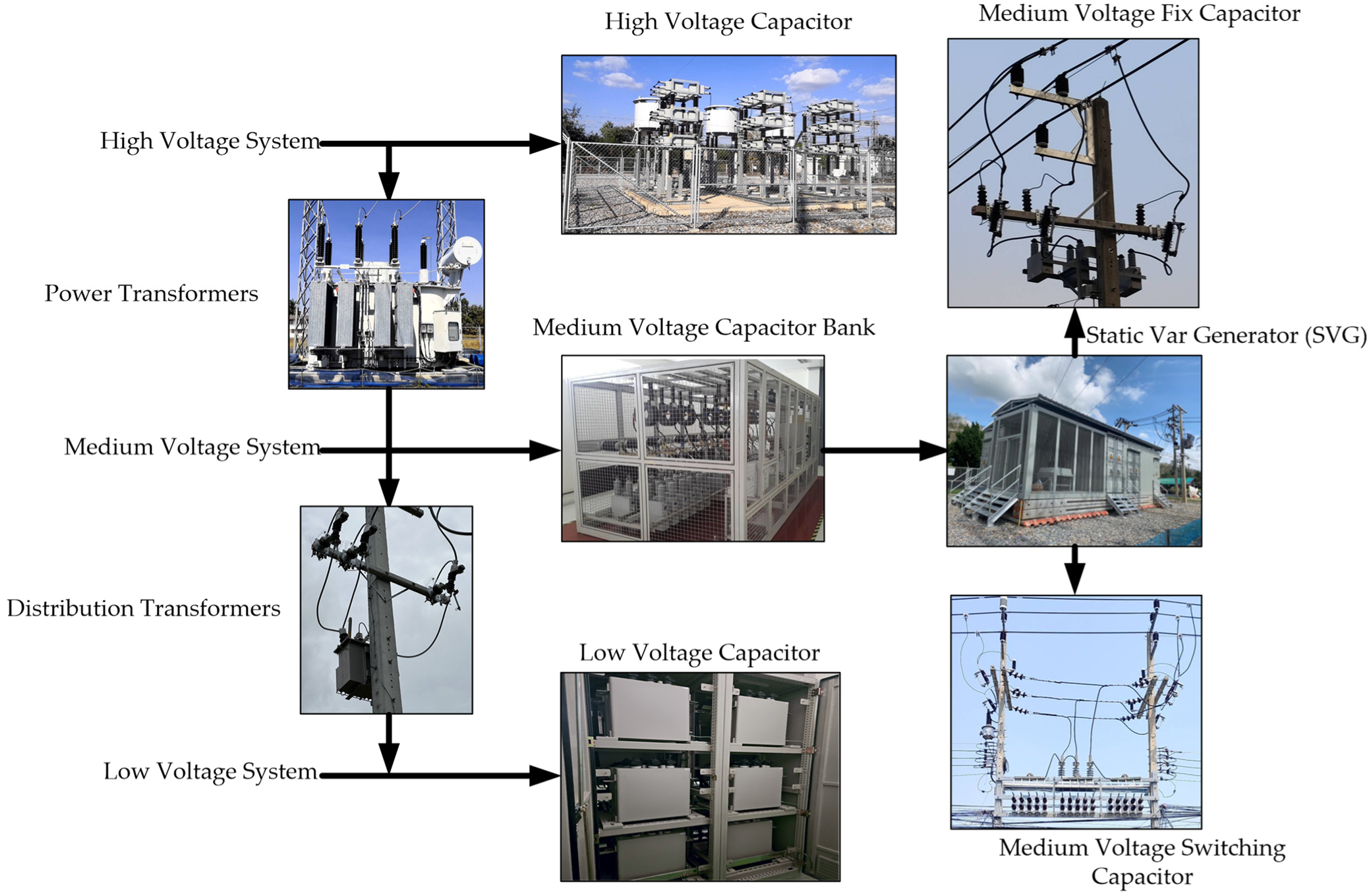
2.1. Type of Capacitor

In this study, the classification of capacitors based on their voltage rating is categorized according to their ability to withstand operating voltages. This can be divided into three main types of reactive compensators, as presented in Figure 1 [13].

Figure 1 shows the position or location of the capacitor installed in an electrical power system. The possible positions are defined using voltage levels for high-voltage, medium-voltage, and low-voltage systems. Therefore, the location of capacitors is a key factor for improving voltage stability and economic costs.

2.2. Possible Installation Positions for Capacitors in Distribution Systems

Research in various studies has shown that the proper installation of capacitors in electrical systems is crucial for maximum benefits. In general, the most suitable locations for capacitor installation are shown in Figure 2 [13].

Figure 1 shows the possible capacitor installation positions. Figure 2i presents the capacitors installed near the root node at power sources or substations. Figure 2ii presents the capacitors installed at the center of the load group. Moreover, Figure 2iii presents the capacitors installed at the end of transmission lines. However, the optimal capacitor placement still needs to be found and solved relative to optimal conditions. Simultaneously, the power flow equations that relate to the capacitors, photovoltaics, and fast charging of electric vehicles and loads are as follows [14]:

$$P_i^{Grid}+P_i^{PV}-P_i^{FCS-EV}-P_i^{load}=\sum _{j=1}^N\left|V_i\right|\left|V_j\right|\left(G_{ij}\cos {\theta }_{ij}+B_{ij}\sin {\theta }_{ij}\right)$$

(1)

$$Q_i^{Grid}+Q_i^{PV}+Q_i^{FCS-EV}+Q_i^{load}-Q_i^C=\sum _{j=1}^N\left|V_i\right|\left|V_j\right|\left(G_{ij}\sin {\theta }_{\mathit{ij}}-B_{ij}\mathrm{c}\mathrm{o}\mathrm{s}{\theta }_{ij}\right)$$

(2)

where $P_i^{Grid}$ and $Q_i^{Grid}$ denote the active and reactive power of the grid at bus $i$. $P_i^{PV}$ and $Q_i^{PV}$ denote the active and reactive power generated by DG at bus $i$. $P_i^{FCS-EV}$ and $Q_i^{FCS-EV}$ denote the active and reactive power consumed by FCS-EV on bus $i$. $P_i^{load}$ and $Q_i^{load}$ denote the active and reactive power consumed by the load at bus $i$. $Q_i^C$ denotes the reactive power of capacitors at bus $i$.

3. Literature Reviews

The proliferation of fast-charging stations (FCSs) for electric vehicles (EVs) has introduced new challenges with respect to the stability and efficiency of power distribution networks. The high-power demand and unpredictable nature of these charging stations can result in voltage fluctuations, power quality deterioration, and potential grid overloading. Conventional approaches to mitigating these issues, such as upgrading transformers and increasing conductor sizes, are often expensive and time-consuming. Consequently, alternative strategies leveraging capacitor placement and renewable energy resources have gained significant attention as cost-effective solutions for maintaining grid stability and resilience.

To explicitly define the problem, FCS integration often results in voltage deviations that exceed acceptable limits (±5% of nominal voltage), increased power losses (up to 15% in high-penetration scenarios), and severe power quality disturbances—such as harmonics and flicker phenomena. These effects necessitate advanced voltage regulation mechanisms to sustain network reliability and efficiency.

Numerous studies have explored capacitor placement as a voltage control mechanism in power distribution networks. Falaghi et al. [15] proposed a risk-based capacitor placement strategy to mitigate voltage deviations and reduce power losses. While economic savings of approximately USD 7000 per year from reduced energy losses are reported, specific percentage improvements in voltage magnitudes or loss reductions are not provided. This study incorporates load uncertainty, uses fuzzy logic to assess voltage violation risk, and considers both constant and switching capacitors, aiming to minimize investment, installation, and energy loss costs. Similarly, Zanganeh et al. [16] introduced a multi-area distribution-grid-optimization framework utilizing D-FACTS devices to enhance power quality and minimize losses. In multi-area operations, real power losses decreased significantly from 580 kW to 320 kW, highlighting improved efficiency. The minimum voltage in the IEEE 33-bus system increased from 0.9871 p.u. to 0.9904 p.u., indicating enhanced voltage stability. Similarly, in the IEEE 13-bus system, the lowest voltage improved from 0.9723 p.u. under single-area operations to 0.9846 p.u. with multi-area operations. Moreover, Parvaneh et al. [17] investigated the integration of capacitor bank placement with demand response programs to improve the operational efficiency of isolated microgrids. The proposed method reduces the real power loss from 86.6 kW to 32.1 kW and reactive loss from 42.4 kVar to 14.9 kVar, exhibiting a nearly 50% improvement compared to previous studies. The voltage magnitude improvement with respect to the minimum voltage improved from 0.967 p.u. (no capacitors) to 0.987 p.u. using different capacitor placements, indicating enhanced voltage stability. In addition to capacitor placement, renewable energy integration plays a crucial role in voltage regulation. However, its intermittent nature often exacerbates voltage instability if not optimally controlled. Mohamed El-Saeed et al. [18] emphasized the need for coordinated control between capacitors and renewables to achieve stable voltage profiles. Their study showed that optimal capacitor placement in RDNs reduces real power loss by up to 32.37% (33-bus) and 31.10% (94-bus) and reactive power loss by 31.79% and 30.49%. Financially, annual net savings reached USD 23,612 with fixed capacitors and USD 23,131 with switched capacitors in a 33-bus system, confirming both technical and economic benefits. Masood et al. [19] explored optimal capacitor placement strategies in the Bangladesh transmission network, demonstrating considerable voltage profile enhancements. Their proposed method lowers reactive power demands to 630 MVAR, achieving reductions of 90 MVAR compared to using fuzzy relational clustering with a genetic algorithm (FRC-GA). Capacitors at buses 6, 7, 8, and 12 keep voltages within 0.95–1.05 p.u., with a maximum improvement of 16.09% at bus 7 and a 4.29% average across the system. Jones et al. [20] examined capacitor placement in large-scale power distribution systems, incorporating load-tap-changing transformer control and revealing its potential to mitigate renewable-energy-induced voltage fluctuations. The use of multi-objective optimization losses is reduced by allowing higher tap settings without voltage violations. Voltage variations in T2 sub-circuits decreased by up to 63%, enhancing stability. Capacitor ratings are reduced by 70% in T1 sub-circuits and 42% in T2 sub-circuits without performance loss. T3 sub-circuits require more investment to achieve similar benefits, highlighting the value of strategic planning. Simultaneously, Peprah et al. [21] analyzed reactive power support in solar PV prosumer grids, highlighting its role in voltage regulation and stability enhancement. Reactive power support in solar PV prosumer grids significantly improves system performance. The total power loss (TPL) decreased from 76.52% to 34.04%, with active and reactive losses reduced to 5.523 kW and 2.718 kW, respectively, after PV injection. Voltage magnitudes also improved; under unbalanced loads, the minimum voltage increased from 0.97 p.u. to 0.98 p.u. with PV and static compensator support. Among different phases, phase B exhibited the best voltage profile, confirming the benefits of integrated PV and reactive power support. Other significant contributions include a two-stage optimization approach for distributed generation and capacitor placement proposed by Mouwafi et al. [22], presenting a two-stage method for the optimal placement of DGs and capacitors and resulting in significant reductions in real power loss and improvements in voltage stability. This is the lowest total real power loss among all scenarios, outperforming previous methods. Voltage magnitudes were improved across different cases, with average values of 0.9884 to 0.9925. Simultaneously, a Hybrid-Gray-Wolf-Optimizer-based capacitor placement technique was proposed by Jayabarathi et al. [23]. In a 34-bus system, HGWO achieved a power loss of 158.57 kW with nine capacitors, providing improvements over the Fuzzy method (162 kW) that are close to the results obtained via mixed-integer nonlinear programming (157.53 kW with six capacitors). The initial post-optimization voltage was expected to stay within 0.9–1.1 p.u. Statistical analyses over 50 runs confirmed HGWO’s consistency and effectiveness. Furthermore, a Shannon’s entropy-based capacitor allocation strategy was proposed by Gupta et al. [24]. Among the methods, the voltage stability index (VSI) exhibited better loss reductions, while the vector index (PLI) improved voltage profiles. Shannon’s entropy index method (SE-IM) yielded the best overall performance. Post-placement, minimum and maximum voltages improved across the network. Additionally, the methods resulted in annual cost savings due to reduced losses, confirming both technical and economic benefits. Furthermore, Gallego et al. [25] introduced a mixed-integer linear programming model that simultaneously optimizes network reconfiguration and capacitor bank placement. Their study demonstrated that optimal capacitor placement and network reconfiguration significantly reduced power losses and enhanced voltage profiles. In a 136-bus system, power loss costs decreased from USD 92,213 to USD 85,876 without investment. Installing the capacitor bank at 1500 kVar yielded a 21.64% loss reduction at a cost of USD 19,550. Overall, power loss reductions ranged from 21.12% to 68.93% across test systems. The minimum voltage magnitudes improved between 0.9714 and 0.9729 p.u., enhancing stability and reliability. Further advancements include the research of Nguyen et al. [26], who developed a hybrid neural network algorithm for the multi-objective optimization of distributed generation and capacitor banks in radial networks. Their study showed that integrating non-dispatchable PV and wind DGs significantly reduces annual energy losses in distribution networks. The proposed symbiosis organism search and neural network algorithm (SOS-NNA) can improve voltage magnitude and stability, which are crucial for reliable system operation under load imbalances and poor regulation. Enhancements in the voltage stability index further confirm improved network resilience. Additionally, SOS-NNA improves branch load balancing, contributing to reduced losses and voltage deviations. These results underscore the effectiveness of combining renewable DGs with intelligent optimization for enhanced power system performance. Mtonga et al. [27] applied the multiverse optimizer to determine optimal shunt capacitor placement and sizing. Their study highlights the use of loss sensitivity factors (LSFs) to identify optimal capacitor placement for minimizing power losses and improving voltage profiles. Normalized bus voltages help reduce the search space, focusing on areas needing voltage support. Identifying critical buses enables targeted capacitor installation with maximum impact on loss reduction and voltage enhancement. In test cases such as the IEEE 69-bus system, real and reactive power losses are 224.89 kW and 102.12 kVar, respectively, serving as performance benchmarks. In contrast, Martins et al. [28] proposed a three-level optimization framework for capacitor allocation in unbalanced systems, demonstrating its effectiveness in voltage stability improvements. The three-level optimization framework effectively minimizes energy loss due to reactive power issues. The voltage profiles across the network also improved, ensuring more stable and reliable operation. This approach was validated on five systems, including IEEE 4-node, 13-node, 37-node, and 123-node feeders, demonstrating consistent performance and robustness. Furthermore, Yinzhang Peng et al.’s [29] study proposed a combined reactive power compensation system by integrating a static var generator (SVG) and a shunt capacitor bank to enhance voltage stability in wind-power-gathering areas. The SVG alone limits voltage dips to 0.134 p.u., improving by 0.032 p.u. over the uncompensated case. Additionally, the combined setup suppresses post-fault oscillations more effectively than SVG alone while supporting transient voltage stability. Optimal device placement and parameter tuning are achieved using modal analysis and improved particle swarm optimization. In contrast, Shuya Tian et al. [30] introduced the optimized sites and sizes of VDAPFs and SVGs using particle swarm optimization (PSO), highlighting the role of SVGs in enhancing voltage stability and power quality in distribution networks. SVGs provide reactive power support, effectively mitigating voltage deviations and harmonics. Two allocation strategies (Allocation 1 and 2) are proposed based on dominant node identification to optimize SVG siting and sizing for cost-effective voltage and harmonic control. An integrated evaluation index assesses SVG performance across economic and power quality criteria. The results show that SVGs significantly reduce voltage deviation and total harmonic distortion (THDV). Future studies are recommended to address uncertainties in power quality disturbances and dynamic allocation strategies.

This study uniquely contributes to the field by selecting IGWO as the optimization technique due to its superior balance between exploration and exploitation. IGWO enhances the search for optimal capacitor and renewable placement by mimicking social leadership hierarchies. This method is particularly advantageous for large-scale distribution networks with high FCS penetration.

To provide real-world context, case studies indicate that cities with rapidly increasing EV adoption, such as Los Angeles and Shenzhen, have reported significant grid instability due to high FCS penetration. Traditional voltage regulation methods have struggled to cope with the fluctuating nature of FCS loads, further reinforcing the necessity for advanced optimization frameworks.

Although these studies have demonstrated the importance of capacitor placement for voltage control, a research gap remains in comprehensively integrating capacitor placement with renewable energy optimization to enhance overall grid resilience. By addressing this limitation, this study proposes a hybrid optimization framework that strategically combines capacitor placement and renewable energy resources to optimize voltage stability in distribution networks with high-penetration FCS.

From

Table 1. Comparison of existing methods based on optimization and control techniques.

Highlights and Brief Details	SVG	UC	RC	FC	CO	PS	VS	TL	VI	EL	AV	UF	SP	MP	CM	OB	OPT	PM	Ref.
Economic savings of USD 7000 per year	-	-	✓	✓	✓	-	-	✓	✓	✓	-	-	✓	-	CC	MO+MS	NSGA-II	BP	[15]
-	-	-	-	✓	✓	-	-	-	✓	✓	-	-	-	✓	HC	MO+MS	MPSO	BP	[16]
Reduces power losses from 86.6 kW to 32.1 kW; improved voltage from 0.967 to 0.987 p.u.	-	-	✓	-	-	-	-	-	✓	✓	-	-	-	✓	CC	MO+MS	HSA	BP	[17]
Reduces power losses by 32.37% (33-bus) and 31.10% (94-bus); economic savings from USD 23,612 to USD 23,131 (33-bus).	-	-	-	✓	✓	-	✓	-	-	-	-	-	✓	-	CC	MO+MS	NSGA-II	BP	[18]
Reduces power losses by 90 MVAR; improved voltage	-	-	✓	-	-	-	-	-	✓	✓	-	-	✓	-	CC	SO	MILP	BP	[19]
-	-	-	✓	-	-	-	-	-	✓	✓	✓	-	✓	-	CC	MO+MS	NSGA-III	BP	[20]
Reduces power losses from 76.52% to 34.04%; improved voltage from 0.97 to 0.98 p.u.	-	-	-	✓	-	✓	-	-	✓	✓		✓	✓	-	DC	MS	FBM	UP	[21]
Improved average voltage from 0.9884 to 0.9925 p.u.	-	-	✓	-	-	-	✓	-	✓	✓	-	-	✓	-	DC	MS	CBA	BP	[22]
Reduces power losses from 158.57 to 157.53 kW	-	-	✓	-	✓	-	-	-	✓	✓	-	-	✓	-	DC	MS	HGWO	BP	[23]
-	-	-	✓	-	✓	-	-	-	✓	✓	-	-	✓	-	DC	MS	SE-IM+ PSO	BP	[24]
Improved voltage to 0.9729 p.u.; economic savings of USD 85,876	-	-	✓	-	✓	-	-	-	✓	✓	-	-	✓	-	DC	MS	MILP	BP	[25]
-	-	-	✓	-	✓	-	✓	-	✓	✓	-	-	✓	-	DC	MO	SOS-NNA	BP	[26]
Reduces power losses to 224.89 kW; normalized bus voltages to 0.95	-	-	✓	-	✓	-	-	-	-	✓	-	-	✓	-	DC	MS	MVA	BP	[27]
	-	-	-	-	-	-	-	-	-	✓	-	-	-	✓	DC	MS	GA	UP	[28]
Improved voltage to 0.032 p.u.	✓	-	✓	-	✓	-	✓	-	-	-	-	-	✓	-	CC	MS	IPSO	BP	[29]
-	✓	-	-	-	-	-	-	✓	-	-	-	-	✓	-	DC	SO	PSO	BP	[30]
-	✓	✓	✓	-	✓	✓	✓	✓	✓	✓	✓	✓	✓	✓	HC	HO	IGWO	UP	Proposed

Remark: PM = Power flow method; BP = balanced power flow; UP = unbalanced power flow; OPT = optimization techniques; GA = genetic algorithm; PSO = particle swarm optimization; IGWO = improved gray wolf optimization; WOA = whale optimization algorithm; NSGA-II = non-dominated sorting algorithm II; MPSO = modified particle swarm optimization; HAS = harmony search algorithm; MILP = mixed-integer linear programming; NSGA-III = non-dominated sorting algorithm III; FBM = forward and backwards method; HGWO = hybrid gray wolf optimizer; SE-IM = novel Shannon’s entropy-based index method; VIIA = variable inclusion and inter-change algorithm; CBA = chaotic bat algorithm; OB = objective function type; SO = single-objective function; MO = multi-objective function; MS = modified single-objective function; HO = hybrid objective function; CM = control method; DC = distributed control; CC = centralized control; HC = hybrid control; AI = machine learning control; MP = multi-period power flow; SP = single-period power flow; UF = unbalanced voltage factor; AV = average voltage factor; VI = voltage deviation index; EL = energy loss; TL = total power loss; vs. = voltage stability index; PS = peak shaving; CO = cost control and economics; FC = fixed-point capacitor placement; R = randomized-point capacitor placement; UC = unbalanced capacitor placement; SVG = static var generator.

, which shows a comparison of 16 previous approaches, it can be observed that most focus on balanced power flow (BP); use traditional algorithms (e.g., NSGA-II, PSO); and only support some technical goals, such as optimizing multi-period power flow (MP), single-period power flow (SP), or the voltage deviation index (VI). Our proposed approach has the following key features: It supports unbalanced power flow (UP), which is more complicated; uses a newly developed improved gray wolf optimization (IGWO) algorithm; uses a hybrid control (HC) network for increased flexibility; and supports 13 out of 14 main technical goals, such as optimizing loss, stability, imbalance, uncertainty, and costs. Therefore, our approach is the most comprehensive compared to previous research and is suitable for modern distribution systems with high complexity.

4. Summary of Major Contributions

This study presents several key contributions to the field of distribution system optimization and renewable energy integration:

• It develops an optimization framework based on improved gray wolf optimization (IGWO) for the optimal placement and sizing of capacitors under both balanced and unbalanced network conditions, incorporating renewable energy sources to enhance voltage performance and system efficiency.
• A comprehensive voltage resilience analysis is carried out under high-penetration fast-charging electric vehicle stations (FCSs), addressing the voltage fluctuations and quality issues associated with increased EV load demands.
• This study implements a hybrid objective optimization model designed to minimize real and reactive power losses, capacitor installation costs, cumulative voltage deviations (CVDs), the voltage unbalance index ($VUI$), and the total QuadTerm and ensure voltage average compliance ($V_{avg}$), providing a holistic view of system performance.
• Validation is carried out using the unbalanced IEEE 123-bus distribution system, demonstrating the robustness and applicability of the proposed IGWO-based framework under realistic network conditions with varying control strategies and renewable integrations.

To further elaborate on these contributions, the rest of this study is organized as follows. Section 2 presents the problem formulation, outlining optimization objectives and constraints. Section 3 details the proposed methodology, including the optimization techniques used for capacitor placement and renewable energy methods. Section 4 discusses the results and provides an in-depth analysis of the simulation’s outcomes. Finally, Section 5 concludes this study and highlights potential future research directions.

5. Problem Formulation of the Proposal

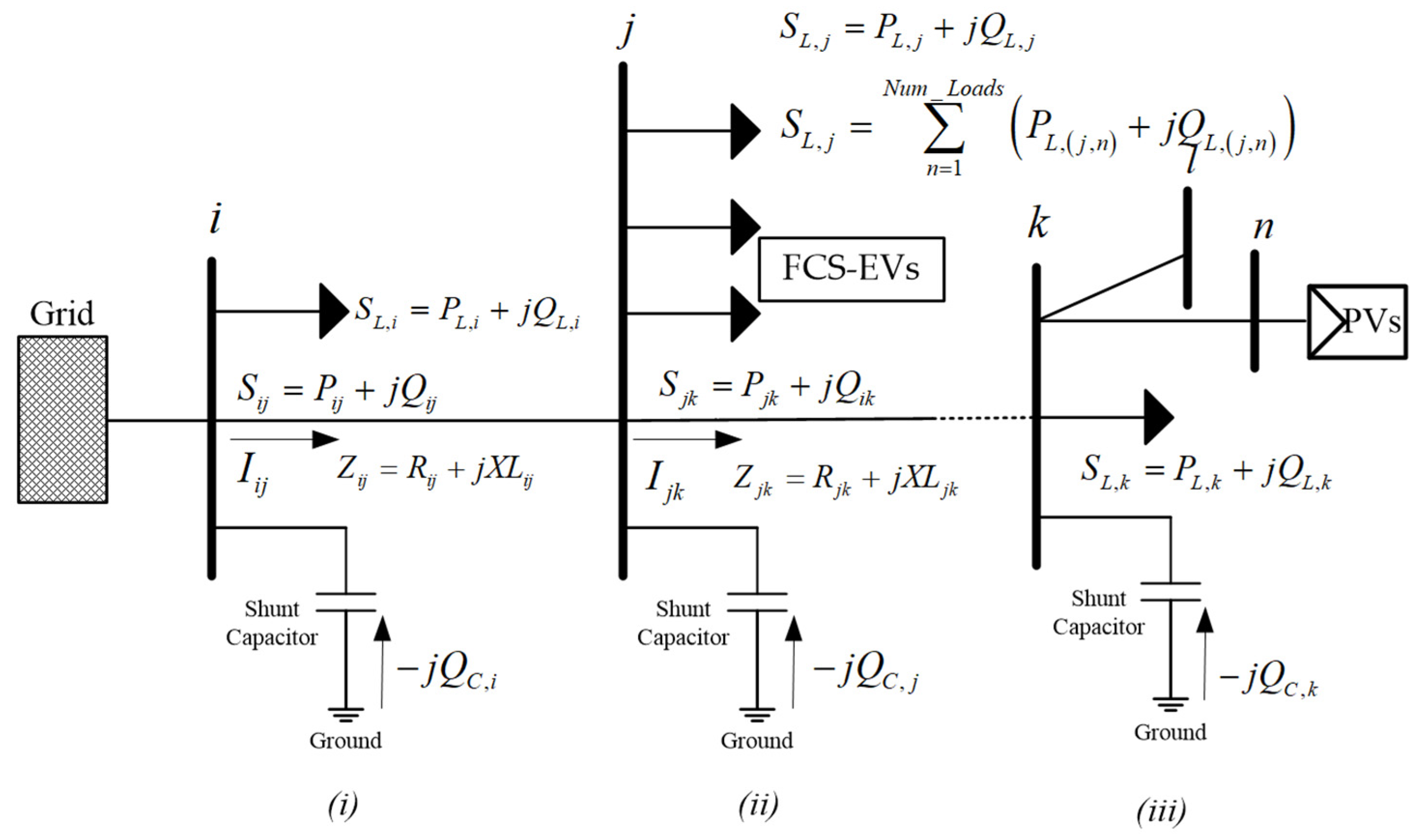
5.1. Unbalanced Power Flow Methodology

The unbalanced power flow $\left(UPF\right)$ equation is an equation used to analyze power systems that have phase imbalances. It is usually solved using the Newton–Raphson method (NR). For each bus in the power system, phases a $a,b,$ and $c$ are considered separately, and the power flow equations for each phase can be written as follows [31].

$$S_i^{\varnothing }=P_i^{\varnothing }+Q_i^{\varnothing }={V_i^{\varnothing }\left(\sum _{k=1}^n\sum _{\phi \in \left\{a,b,c\right\}}{Y}_{ik}^{\varnothing \phi }{V}_k^{\phi }\right)}^{*}$$

(3)

The complex power equation for phase $\varnothing \in \left\{a,b,c\right\}$ is shown, where $S_i^{\varnothing }$ denotes complex power at bus $i$ and phase $\varnothing$ (when $P_i^{\varnothing }$ is the active power; $Q_i^{\varnothing }$ is the reactive power); $V_i^{\varnothing }$ is the voltage at bus $i$ and phase $\varnothing$ (in polar form: $V_i^{\varnothing }=\left|V_i^{\varnothing }\right|\angle {\theta }_i^{\varnothing }$); $Y_i^{\varnothing \phi }$ is the admittance matrix element between the phase $\varnothing$ of bus $i$ and the phase $\phi$ of bus $k$; and $n$ denotes the number of buses in the system.

$$P_i^{\varnothing }=\left|V_i^{\varnothing }\right|\sum _{k=1}^n\sum _{\phi \in \left\{a,b,c\right\}}\left|V_k^{\phi }\right|\left[G_{ik}^{\varnothing \phi }cos\left({\theta }_i^{\varnothing }-{\theta }_k^{\phi }\right)+B_{ik}^{\varnothing \phi }sin\left({\theta }_i^{\varnothing }-{\theta }_k^{\phi }\right)\right]$$

(4)

$$Q_i^{\varnothing }=\left|V_i^{\varnothing }\right|\sum _{k=1}^n\sum _{\phi \in \left\{a,b,c\right\}}\left|V_k^{\phi }\right|\left[G_{ik}^{\varnothing \phi }sin\left({\theta }_i^{\varnothing }-{\theta }_k^{\phi }\right)-B_{ik}^{\varnothing \phi }cos\left({\theta }_i^{\varnothing }-{\theta }_k^{\phi }\right)\right]$$

(5)

Here, active and reactive power equations are shown, where $G_{ik}^{\varnothing \phi }$ and $B_{ik}^{\varnothing \phi }$ are the conductance and susceptance of the admittance matrix.

5.1.1. Total Power Loss and Reactive Power Loss

In an unbalanced three-phase system, the power loss can be calculated as the sum of losses in each phase (a, b, and c) and the losses due to the inter-phase imbalance. The loss in each phase is calculated as the difference between the power injected and power delivered at each bus:

$$P_{loss}^{\varnothing }=\sum _{i=1}^n\left(P_{i,inj}^{\varnothing }-P_{i,load}^{\varnothing }\right)$$

(6)

$$Q_{loss}^{\varnothing }=\sum _{i=1}^n\left(Q_{i,inj}^{\varnothing }-Q_{i,load}^{\varnothing }\right)$$

(7)

where $P_{i,inj}^{\varnothing } \mathrm{a}\mathrm{n}\mathrm{d} Q_{i,inj}^{\varnothing }$ are the real and reactive power delivered to bus $i$ in phase $\varnothing .$ $P_{i,load}^{\varnothing } \mathrm{a}\mathrm{n}\mathrm{d} Q_{i,load}^{\varnothing }$ are the load active and reactive power at bus $i$ in phase $\varnothing .$

$$P_{loss,ij}^{\varnothing }={\left|I_{ij}^{\varnothing }\right|}^2{R}_{ij}^{\varnothing }$$

(8)

$$Q_{loss,ij}^{\varnothing }={\left|I_{ij}^{\varnothing }\right|}^2{X}_{ij}^{\varnothing }$$

(9)

The transmission line loss between buses $i$ and $j$ in each phase is calculated from the current line and resistance (8,9). Here, $I_{ij}^{\varnothing }$ is the current in phase $\varnothing$ of the line between buses $i$ and $j.$ Thus, $R_{ij}^{\varnothing }$ and $X_{ij}^{\varnothing }$ are the resistance and reactance of phase line $\varnothing$, and admittance matrix $Y_{ij}^{\varnothing \phi }$ is used between phases $\varnothing$ and $\phi \left(10\right)$.

$$I_{ij}^{\varnothing }=\sum _{\phi \in \left\{a,b,c\right\}}{Y}_{ij}^{\varnothing \phi }\left(V_i^{\varnothing }-V_j^{\phi }\right)$$

(10)

Therefore, the total real power loss and reactive power loss equations are as follows.

$$P_{loss,total}=\sum _{\varnothing \in \left\{a,b,c\right\}}\sum _{i=1}^n\sum _{j\in neighbors\left(i\right)}{P}_{loss,ij}^{\varnothing }$$

(11)

$$Q_{loss,total}=\sum _{\varnothing \in \left\{a,b,c\right\}}\sum _{i=1}^n\sum _{j\in neighbors\left(i\right)}{Q}_{loss,ij}^{\varnothing }$$

(12)

5.1.2. Commutative Voltage Deviation (CVD)

The commutative voltage deviation $\left(CVD\right)$ is the average voltage deviation of each phase. It can be calculated using the difference in the voltage magnitude at each bus and the voltage reference of the system as follows:

$$CVD=\left[{\displaystyle \frac{\sum _{i=1}^n\left|V_i^{\varnothing }-V_{ref}\right|}{n}}\right]$$

(13)

where $V_{ref}$ is the voltage reference equal to 1 p.u., and $n$ is the number of buses.

5.1.3. Total Quadratic Term (Total QuadTerm) of Control Voltage Tolerance

The control voltage tolerance of the electrical power system is used to set the voltage magnitude level under the underload variations of each bus. The summation of the voltage for each bus’s underload variation indicates the voltage magnitude level under or over the standard control, and it is calculated as follows:

$$\mathrm{T}\mathrm{o}\mathrm{t}\mathrm{a}\mathrm{l}\mathrm{Q}\mathrm{u}\mathrm{a}\mathrm{d}\mathrm{T}\mathrm{e}\mathrm{r}\mathrm{m}\left(V_{\varnothing }\right)={\sum }_{i=1}^n\begin{array}{cc}{\left(V_i-V_{min}\right)}^2& if V_i<V_{min}\\ {\left(V_i-V_{max}\right)}^2& if V_i>V_{max}\\ 0& otherwise\end{array}$$

(14)

where $V_i$ is the voltage bus. $V_{min}$ and $V_{max}$ are the control voltage ranges of the 0.95–1.05 p.u. bus. $n$ is the number of buses.

5.1.4. Voltage Average $\left({\mathrm{V}}_{\mathrm{a}\mathrm{v}\mathrm{g}}\right)$

The voltage average $\left(V_{avg}\right)$ describes the difference between each phase’s voltage at any bus. $V_{avg}$ is used to consider the system’s voltage equality, and it is one of the methods used to assess the balance condition of the electrical system. $V_{avg}$ can be represented as follows:

$$V_{avg}={\displaystyle \frac{1}{3}}\sum _{i=1}^n{V}_i^{\varnothing }$$

(15)

where $V_{avg}$ is the voltage average at bus $i$. $\varnothing$ is the phase sequence described via $\varnothing \in \left\{a,b,c\right\}$.

5.1.5. Voltage Unbalance Index (VUI)

In the static-state simulation, this study utilized the IEEE 123-bus test system (in which single-phase, two-phase, and three-phase configurations are mixed) for simulation purposes, and the respective magnitude of the voltage unbalance index $(VUI$) is defined as follows:

$$VUI=max\left|{\displaystyle \frac{V_i^{\varnothing }-V_{avg}}{V_{avg}}}\right|·100$$

(16)

5.1.6. Environmental Performance Indices (EPIs)

Environmental performance indices (EPIs) are related to the reduced power generation achieved by using green energy. This research focuses on PV power generation, which is generated within a solar period at an average of 4.5 hr. per day. The reduced power loss is caused by the capacitor’s time period at an average of 19.5 hr. per day. However, broader environmental aspects, such as land use for PV installations and EV battery degradation, are beyond the scope of this study. Our focus is limited to CO₂ emissions that directly relate to power loss and renewable energy integration. The EPIs are represented as follows [32]:

$${CO}_2=\left[\left(\left(PV{+Ploss}_{\left(Reduce\right)}\right)·T_{PV}·E \right){+(Ploss}_{\left(Reduce\right)}·T_C)\right]·360 day/y$$

(17)

where $T_{PV}$ is the peak sun hour: 4.5 hr. per day. $T_C$ is the time period of the capacitor’s operation: 19.5 hr. per day. $E$ is the emission factor of the Thailand voluntary emission reduction program (T-VER), which is equal to 0.5251 $t{CO}_2/MWh$.

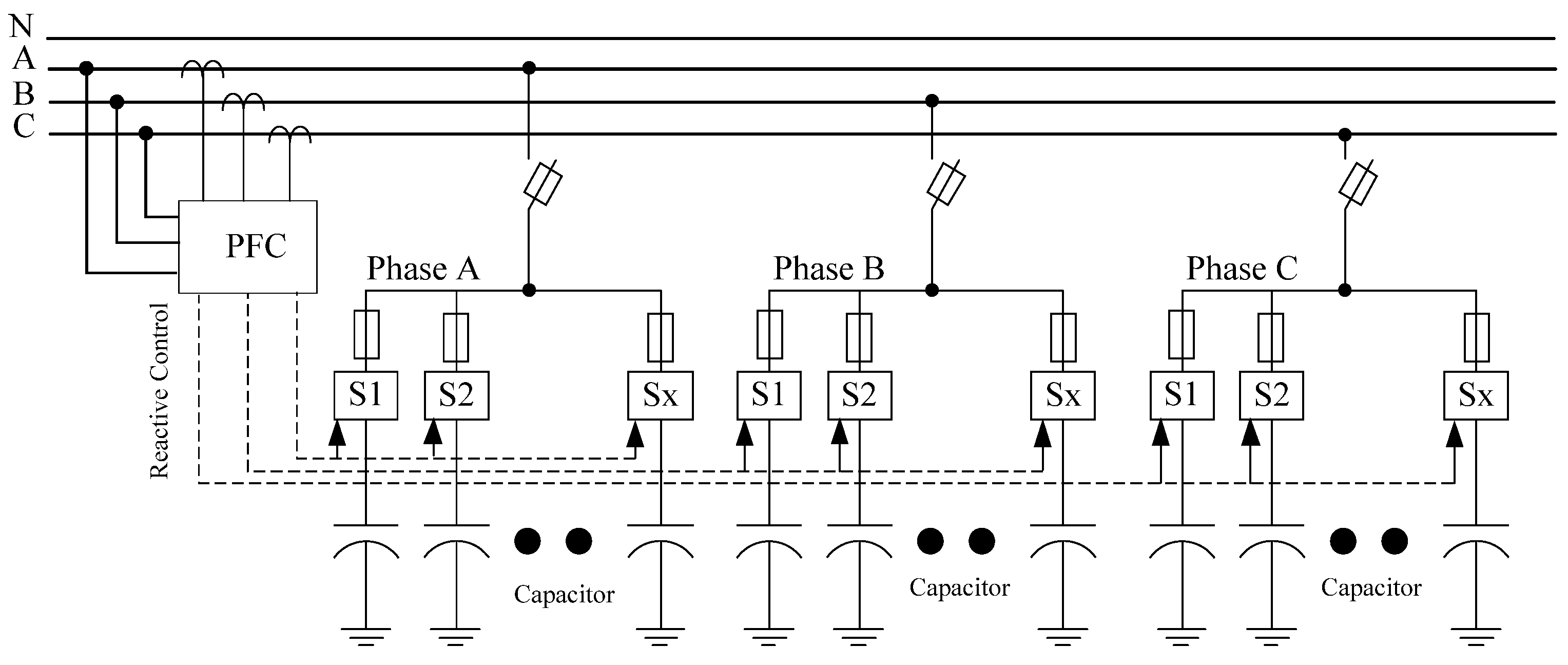
5.2. Unbalanced Control of Capacitor Steps

The control diagram of capacitors consists of the power factor controller, switch or contractor, and capacitors. The reactive compensation of capacitors can operate under dependency and generate reactive power via stepping operations relative to the required power system [19]:

$$\left.\begin{array}{c}{Q}_A=Q_{C1,A}·S_1+Q_{C2,A}·S_2+Q_{Cx,A}·S_x\\ Q_B=Q_{C1,B}·S_1+Q_{C2,B}·S_2+Q_{Cx,B}·S_x\\ Q_C=Q_{C1,C}·S_1+Q_{C2,C}·S_2+Q_{Cx,C}·S_x\end{array} \right\} ;S_1, S_2,S_x\in \left\{0, 1\right\}$$

(18)

where $Q_{C1,A,B,C}$ is the reactive power of capacitor set 1 $\left(S_1\right)$ of phases $A, B, \mathrm{a}\mathrm{n}\mathrm{d} C$;

$Q_{C2,A,B,C}$ is the reactive power of capacitor set 2 $\left(S_2\right)$ of phases $A, B, \mathrm{a}\mathrm{n}\mathrm{d} C$;

$Q_{Cx,A,B,C}$ is the reactive power of capacitor set $x$ $\left(S_x\right)$ of phases $A, B, \mathrm{a}\mathrm{n}\mathrm{d} C$.

$$Q_{\varnothing }={\sum }_{i=1}^n{Q}_{Ci,\varnothing }·S_i \mathrm{for} \varnothing \in \left\{A,B,C\right\}$$

(19)

Here, $i$ is the number of capacitor steps.

Figure 3 illustrates the schematic of an unbalanced capacitor control system designed for phase-wise reactive power compensation. Each phase (A, B, C) is equipped with independently switchable capacitor banks (S1, S2, Sx), allowing the power factor controller (PFC) to selectively regulate reactive power based on unbalanced load conditions. This configuration enhances voltage profile stability and minimizes unbalanced across the network phases.

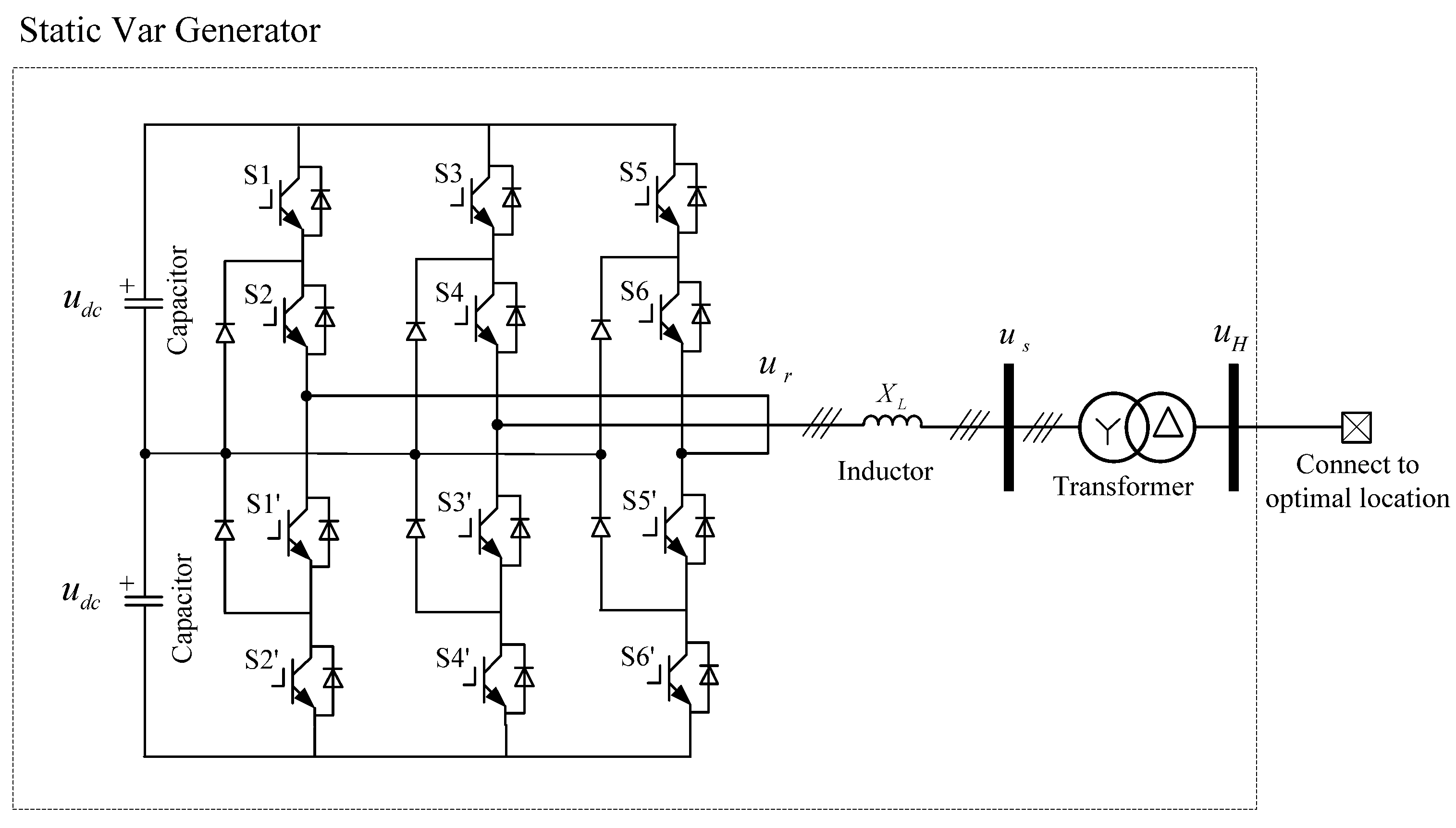
5.3. Static Var Generator (SVG)

The SVG is shown in Figure 4. It is connected to the high-voltage side of the point of common coupling (PCC) via a connection with the transformer and inductor $\left(L\right)$. The SVG outputs a fundamental component voltage $\left(U_r\right)$ at the same frequency as the system voltage $\left(U_s\right)$ through SPWM modulation (or other modulation methods) [33]. The SVG is represented by only compensating the reactive power and generating fine values, which is greater than the unbalanced control of the capacitor step.

If the loss of the connection inductor is ignored, the steady-state power expression of the SVG can be obtained using Equation (21):

$$P_{SVG}={\displaystyle \frac{U_s·U_r}{X_L}}\sin \delta$$

(20)

$$Q_{SVG}={\displaystyle \frac{U_s·\left(U_r\cos \delta -U_s\right)}{X_L}}$$

(21)

The SVG only considers the reactive power, in which real power equals zero, by controlling the power angle of $\delta$. This model is selected in this study, and it can be expressed as follows:

$$Q_{SVG}={\displaystyle \frac{U_s·\left(U_r-U_s\right)}{X_L}}; \delta =0$$

(22)

Therefore, the voltage of $U_s$ can be improved as follows:

$$U_s^2-U_s·U_r+Q_{SVG}·X_L=0$$

(23)

$$U_S={\displaystyle \frac{U_r\pm \sqrt{U_r^2-(4·Q_{SVG}·X_L)}}{2}}; U_r^2-(4·Q_{SVG}·X_L)\ge 0$$

(24)

where $Q_{SVG}$ is the reactive power of SVG. $U_s$ is the voltage magnitude at a common connection point. $U_r$ is the output voltage magnitude of the SVG. $X_L$ is the inductive resistance value of the connection inductor.

5.4. Photovoltaic System Modeling

The distributed energy resources (DERs) are represented by the PV power plant. The active power output of a solar PV system is determined using solar irradiance, temperature, and system efficiency [34]:

$$P_{PVs}\left(t\right)=G\left(t\right)·A_{PVs}·{\eta }_{PVs}$$

(25)

where $P_{PVs}$ is the PV system’s active power output (in MW) at time $t$; $G$ is the solar irradiance (in $\mathrm{k}\mathrm{W}/{\mathrm{m}}^2$) at time $t$; $A_{PVs}$ is the total area of PV panels (in ${\mathrm{m}}^2$); ${\eta }_{PVs}$ is the overall efficiency of the PV system, including the panel, inverter, and system losses. The module’s efficiency ${\eta }_{PVs}$ is temperature-dependent:

$${\eta }_{PVs}={\eta }_{module,STC}\left[1·\beta ·\left(T_c-T_{STC}\right)\right]$$

(26)

where ${\eta }_{module,STC}$ is the module’s efficiency at standard test conditions (STCs). $\beta$ is the temperature coefficient of power ($\%/℃$). $T_c$ is the cell temperature ($℃$). $T_{STC}$ is the standard test condition temperature (25 °C).

The cell temperature $T_c$ can be approximated as follows:

$$T_c=T_a+\left[{\displaystyle \frac{G\left(t\right)}{G_{ref}}}\right]·NOCT$$

(27)

where $T_a$ is the ambient temperature ($℃$).$G_{ref}$ is reference irradiance (typically 1000 $\mathrm{W}/{\mathrm{m}}^2$). $NOCT$ is the nominal operating cell temperature ($℃$).

The reactive power control of PV power plants is used to control the power and voltage of the point of common coupling (PCC). PV can be controlled using PF control, which is related to the reactive power output, and it can be defined as follows:

$$Q_{PVs}=\sqrt{S_{PVs}^2-P_{PVs}^2}$$

(28)

$$Q_{PVs}=P_{PVs}·\tan \left({\cos }^{-1}\left(PF\right)\right)$$

(29)

$$PF=0.85$$

(30)

where $Q_{PVs}$ is the reactive power generated by the PV system (in MVar). $S_{PVs}$ is the apparent power capacity of the PV system (in MVA). $P_{PVs}$ is the active power generated by the PV system (in MW).

5.5. Fast-Charging Station for Electric Vehicles (FCS-EV)

Most of these devices are related via power electronic conversion from AC to DC; they are also called rectifier circuits and connected using a wire conductor to the battery system on electric vehicles. Thus, many researchers have studied the characteristics of FCS-EVs in order to find and analyze the impact of electric vehicles on grids. This research study uses the constant power model of FCS-EVs, as shown in Figure 5 [35].

$$P_i^{FCS-EV}=P_i^{fixed}$$

(31)

$$Q_i^{FCS-EV}=P_i^{FCS-EV}\tan \left({\cos }^{-1}\left(PF\right)\right)$$

(32)

$$PF=0.95$$

(33)

Here, $P_i^{FCS-EV}$ and $Q_i^{FCS-EV}$ are the active and reactive power consumed by FCS-EVs at bus $i$. $P_i^{fixed}$ is the size of the FCS. $PF$ is the power factor of the FCS.

5.6. Improved Gray Wolf Optimization

The gray wolf optimization (GWO) algorithm is inspired by the social leadership and hunting behavior of gray wolves in nature. Wolf hunting consists of three main steps: encircling, hunting, and attacking the prey [36].

Encircling: The encircling stage can be modeled using Equations (34) and (35).

$$D=‖C·X_p\left(t\right)-X\left(t\right)‖$$

(34)

$$X\left(t+1\right)=X_p\left(t\right)-A·D$$

(35)

$$A=2·A·r_1-a\left(t\right)$$

(36)

$$C=2·r_2$$

(37)

$$a\left(t\right)=2-\left(2·t\right)/interation$$

(38)

Hunting: To mathematically model wolves’ hunting behavior, it is assumed that α, β, and δ denote knowledge of the location of the prey.

$$X\left(t+1\right)={\displaystyle \frac{X_{i1}+X_{i2}+X_{i3}}{3}}$$

(39)

Attacking: The hunting process is terminated when the prey stops moving and the wolves start an attack. This can be carried out mathematically using the value of $a$, which decreases linearly over iterations, controlling exploration and exploitation. As shown in Equation (38), it is updated in each iteration to range from 2 to 0.

In this section, an improved grey wolf optimizer (IGWO) is proposed. The improvements include a new search strategy associated with selecting and updating steps. IGWO includes three phases: initializing, movement, and selecting and updating.

Initializing phase: In this phase, N wolves are randomly distributed in the search space in each range of $\left[l_j , u_j\right]$ using Equation (40).

$$X_{ij}=l_j+{rand}_j\left[\mathrm{0,1}\right]·\left(l_j, u_j\right) , i\in \left[1 , N\right] , j\in \left[1 , D\right]$$

(40)

Movement phase: There are two formats in this phase. The canonical GWO search strategy follows the new position of wolf $X_i\left(t\right)$, named $X_{IGWO}\left(t+1\right)$, and it is calculated using equation (41) and the dimension-learning-based hunting (DLH) search strategy:

$$R_i\left(t\right)=‖X_i\left(t\right)-X_{IGWO}\left(t+1\right)‖$$

(41)

$$X_{IDLH,d}\left(t+1\right)=X_{i,d}\left(t\right)+rand·\left(X_{n,d}-X_{r,d}\right)$$

(42)

Selecting and updating phase: In this phase, the superior candidate is first selected by comparing the fitness values of two candidates $X_{IGWO}\left(t+1\right)$ and $X_{IDLH}\left(t+1\right)$ using Equation (43).

$$X_i\left(t+1\right)=\left\{\begin{array}{cc}{X}_{IGWO}\left(t+1\right),& if f\left(X_{IGWO}\right)<f\left(X_{IDLH}\right)\\ X_{IDLH}\left(t+1\right)& otherwise\end{array}\right.$$

(43)

Then, $X_i\left(t+1\right)$ is updated to the new position.

Finally, after performing this procedure for all individuals, the number of iterations is increased by one, and the search can be iterated until a predefined number of iterations is reached. The pseudo-code of the proposed IGWO algorithm is shown in Algorithm 1.

Algorithm 1 Improved Gray Wolf Optimization
	Input: f(x), N, dim, Iteration, LB, UB
	Output: nvar, Fbest
1:	Begin
2:	Initializing (Randomly N wolves in program and calculated of fitness function)
3:	For iter = 2 to Iteration
4:	$\mathrm{Find} {\mathrm{X}}_{\mathsf{\alpha }}$$, {\mathrm{X}}_{\beta }$$\mathrm{and} {\mathrm{X}}_{\delta }$
5:	For i = 1 to N
6:	$\mathrm{Calculation} X_{i1}$, $X_{i2}$, $X_{i3}$
7:	$\mathrm{Calculation} X_{IGWO}\left(t+1\right)$ by using Equation (39)
8:	$\mathrm{Calculation} R_i\left(t\right)$ by using Equation (41)
9:	$\mathrm{Constructing} \mathrm{neighborhood} X_i\left(t\right)$ with radius $R_i\left(t\right)$
10:	For d = 1 to dim
11:	$X_{IDLH,d}\left(t+1\right)$ by using Equation (42)
12:	End for
13:	$\mathrm{Selection} \mathrm{of} \mathrm{the} \mathrm{best} (X_{IGWO}\left(t+1\right)$, $X_{IDLH,d}\left(t+1\right)$)
14:	Updating population
15:	End for
16:	End for
17:	Return nvar, Fbest
18:	End

6. Methodology

Although this study applied analyses for the steady-state case, previous studies utilized unstable analyses [8,9]. The control of a flexible power system used to improve the voltage stability of a power system can also be utilized [11,12]. However, this study focuses on simulation-based analysis using the IEEE 123-bus benchmark system, which is widely accepted for academic and technical evaluation. Future research should consider the use of real operational data to further support our method’s applicability.

6.1. Hybrid Objective Function for Optimization Techniques

The hybrid objective function is formulated to minimize the following: power losses, reactive power loss, commutative voltage deviation $\left(CVD\right)$, $VUI$, total QuadTerm, voltage average ${(V}_{avg})$, and cost of the capacitor. In our study, voltage stability was assessed using the commutative voltage deviation $\left(CVD\right)$, $VUI$, total QuadTerm, and voltage average ${(V}_{avg})$. A specific voltage stability index (VSI) was not used in this study.

The optimization aims to minimize multi-objective function $F$ by combining several goals:

$$\begin{gathered} \min F=\left[w_1·P_{loss,total}+w_2·Q_{loss,total}+w_3·QuadTerm+w_4·CVD+w_5 \\ ·V_{avg}+w_6·VUI+w_7·Cost\right] \end{gathered}$$

(44)

where $P_{loss,total}$ is the total active power loss in the network. $Q_{loss,total}$ is the total reactive power loss in the network. $Total QuadTerm$ is the minimum total number of quadratic programming algorithms. $CVD$ is the commutative voltage deviation. $V_{avg}$ is the voltage average relative to the network. $VUI$ is the voltage unbalance factor in the network. $Cost$ is the installation cost of capacitors. All seven variables were adjusted to p.u. values. $w_1, w_2, w_3, w_4, w_5, w_6, \mathrm{a}\mathrm{n}\mathrm{d} w_7$ are the weights assigned to each objective, which are set up at 0.2, 0.1, 0.1, 0.1, 0.1, 0.3, and 0.1, respectively.

6.2. Inequality Constraint and Limits

6.2.1. The Voltage Magnitude at the Bus Must Remain Within Permissible Limits

$$V_{min}<\left|V_i^{\varnothing }\right|<V_{max} ,\dots \forall i\in Buses$$

(45)

where $\left|V_i^{\varnothing }\right|$ is the absolute voltage magnitude at bus $i$. $V_{min}$ and $V_{max}$ are the minimum and maximum voltage magnitude limits at 0.95 p.u. and 1.05 p.u., respectively.

6.2.2. Load Line Limit

The line load on each transmission line must not exceed its capacity.

$$S_{ij}=\sqrt{P_{ij}^2+Q_{ij}^2} \le S_{ij}^{max},\dots \forall (i,j)\in Line$$

(46)

6.2.3. FCS-EV and Capacitors

The FCS-EV station must consume energy from the grid, and it cannot be installed in the same location as the next FCS-EV station, as shown in as in Equations (47) and (48). Simultaneously, the capacitors cannot be installed at the same position as the capacitors used in Equation (49).

$$P_i^{FCS-EV},Q_i^{FCS-EV}\ge 0$$

(47)

$${\mathbb{Z}}_{FCS-EV}=\left\{s_1,s_2,\dots ,s_N\right\}; s_i\ne s_{j } {\forall }_i\ne j, i,j \in \left\{\mathrm{1,2},\dots N\right\}$$

(48)

$${\mathbb{Z}}_{Capacitors}=\left\{s_1,s_2,\dots ,s_N\right\}; s_i\ne s_{j } {\forall }_i\ne j, i,j \in \left\{\mathrm{1,2},\dots N\right\}$$

(49)

6.2.4. The Power Balance of the Grid Is Considered Relative to the Load Power Demand, the Power Demand of FCS-EV, and the Active Power Output of PV. It Is Described Using Equations (50) and (51)

$$P_{Grid}=P_{load}+P_{FCS-EV}-P_{PV}$$

(50)

$$\begin{gathered} if Q_{\varnothing }<Q_{\varnothing }^{ref}-∆Q \mathrm{then} \mathrm{Turn} \mathrm{ON} \mathrm{next} S_i \\ if Q_{\varnothing }>Q_{\varnothing }^{ref}+∆Q \mathrm{then} \mathrm{Turn} \mathrm{OFF} \mathrm{next} S_i \end{gathered}$$

(51)

where $∆Q$ is the tolerance of the different reactive powers of the grid.

6.2.5. Power Factor (PF) Constraints: The PF of DG Must Remain Within Its Operational Limits as Follows

$${PF}_{min}\le {PF}_N\le {PF}_{max},\dots \forall N\in Number of DG$$

(52)

6.2.6. Renewable Power Output Constraints: The Power Generated by PV Systems Must Re-Spect Resource Availability, Which Is Described as Follows

$$P_{PV}^{min}\le P_{PV}\le P_{PV}^{max},\dots \forall t$$

(53)

6.3. Simulation Parameters

Table 2. Parameters of multi-optimization techniques.

Description	Parameters	Value/Range
Capacitors:
Possible position of capacitor	Cap. Pos.	All buses of three phases
Size of capacitors	Cap. Step Cap. Size	6 steps 25, 50, 75, 100, 125, 150 kVar
Static Var Generator (SVG):
	Pos.	All buses of three phases
		$5\text{–}100 \mathrm{kVar} \text{@} 1\varnothing$
		$15\text{–}300 \mathrm{kVar} \text{@} 3\varnothing$
Voltage set point	Vset.	1 p.u.
Electric Vehicle Fast-Charging Station:
Fast-charging station capacity	FCS Cap.	22, 50, 125, 150, 300 kW
Possible position of FCS-EVs	FCS Pos.	All buses of three phases
Power factor of FCS-EVs	PF	0.95
Photovoltaic System:
PV power plant capacity	PVs Cap.	$15\text{–}500 \mathrm{kVA} \text{@} 1\varnothing$
		$100\text{–}1500 \mathrm{kVA} \text{@} 3\varnothing$
Position of PV power plant	PVs Pos.	bus No. 195, 251, 451
Power factor of PV	PF	0.85
Optimization Algorithm:
Solving the problem limit range	Iteration	100
Improve gray wolf optimization (IGWO):
Number of wolves	N	100

shows the parameters of the multi-optimization techniques used to find optimal conditions. Thus, all basic parameters of each optimization are needed to carry out performance comparisons.

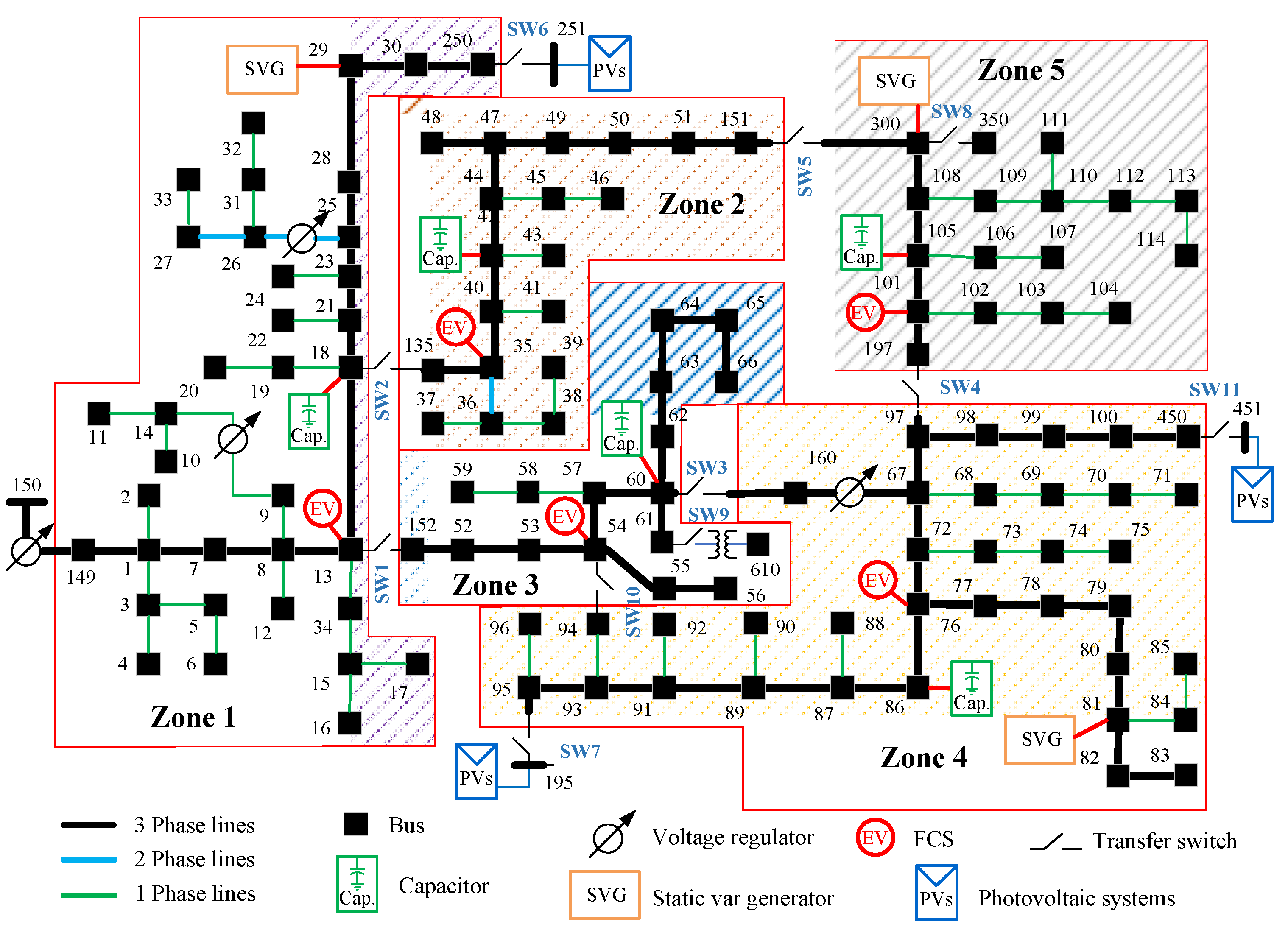
6.4. Modified IEEE 123-Bus Testing System

This study modified the IEEE 123-bus system [37] to apply voltage improvements under different capacitor placements. This electrical power system is an unbalanced system that closely mirrors the complexity of real-world electrical networks. The IEEE 123-bus system was modeled under steady-state conditions using the peak demand of each study case. The analysis involved randomly assigning power values for EVs and capacitors (following IEEE Std 1036-2010 [38]), which should not exceed 40 to 50% of the transformer rating—and PVs (IEEE 1547 [39]), which should not exceed 75 to 100%. This study utilized MATLAB version 2018b along with Open Distribution System Simulator (OpenDSS) interfaces 10.1.0.1 (64-bit build)—Columbus [40] for case analyses, and it can be applied to problems, such as those reported by the authors [41,42,43,44]. The initial simulation parameters were set as follows:

• Many researchers modified the IEEE 123-bus system by dividing the system into zones to solve issues [45,46,47]. Therefore, this research study was defined in accordance with an analysis zone named the All-Zone (AZ) (as shown in Figure 6), which was further divided into 5 zones (Zs) (as shown in

  Table 3. Zone division patterns with five zones and bus identification.

  Zone	Bus (Number)
  1	149, 1, 7, 8, 13, 18, 21, 23, 25, 28, 29, 30, 250
  2	135, 35, 40, 42, 44, 47, 48, 49, 50, 51, 151
  3	152, 52, 53, 54, 55, 56, 57, 60, 62, 63, 64, 65, 66
  4	160, 67, 97, 98, 99, 100, 450, 72, 72, 76, 77, 78, 79, 80, 81, 82, 83, 86, 87, 89, 91, 93, 95
  5	197, 101, 105, 108, 300

  ).
• Previous research focuses on the reactive power compensation using capacitors that are balanced [15,48,49]. Thus, this scenario defined the balanced-phase capacitors with initial values set to 15 to 300 kVar (balanced static var generator, BSVG) using 6-step configurations: 75, 150, 225, 300, and 450 kVar (balanced step capacitor, BSC). The capacitor’s sizing steps (25, 50, and 75 kVar) were selected based on the commonly available standard ratings of practical distribution systems. This ensures that the optimization results are more applicable in the real world.
• Unbalanced-phase capacitors were set to 5 to 100 kVar per phase (unbalanced static var generator for reactive compensation, USVG) with 6-step configurations: 25, 50, 75, 100, 125, and 150 kVar (unbalanced step capacitor, USC).
• FCS-EV (EV) power levels were set at 22, 50, 125, 200, and 300 kW. Each FCS-EV installation is unique and not repeated, with different power capacities allocated to distinct zones based on spatial availability and operational requirements.
• PV locations were assigned to buses 195, 251, and 451 with the following configurations: single-phase PV (PV1P): 30 to 500 kVA with PF = 0.85; and three-phase PV (PV3P) at 100–1500 kVA with PF = 0.85.
• Capacitors, EV, and PV were only installed on three-phase buses, with the condition that each can only occupy one bus.
• The automatic voltage regulators (AVRs) for all transformers were uncontrolled relative to tap adjustments, and existing capacitors were disconnected from the system.

6.5. Definition of the Case Study

To assess the performance of the proposed optimal control strategies under realistic operating conditions, a comprehensive set of case studies was performed using the IEEE 123-bus unbalanced distribution test system. These case studies were designed to evaluate the impact of various control configurations on voltage magnitude levels, energy losses, and system balance across different deployment scenarios.

As summarized in

Table 4. The five defined simulation models and 19 case studies.

Simulation Model	Case	Case Configuration										Case Descriptions
		Base Case (BC)	FCS-EV	PV1P	PV3P	BSVG	USVG	BSC	USC	Zone (Z)	All-Zone (AZ)
1	1	✓										Find values to assess the impact of the base case
	2	✓	✓							✓		Randomize EV values to assess impact
	3	✓			✓							Randomize PV3P values to assess impact
2	4	✓				✓				✓		Randomize BSVG within each zone with CC method
	5	✓				✓					✓	Randomize BSVG across all zones with DC method
	6	✓						✓		✓		Randomize BSC within each zone
	7	✓						✓			✓	Randomize BSC across all zones with DC method
3	8	✓	✓				✓			✓		Randomize USVG and EV within each zone with CC method
	9	✓	✓				✓				✓	Randomize USVG and EV across all zones with DC method
	10	✓	✓						✓	✓		Randomize USC and EV within each zone with CC method
	11	✓	✓						✓		✓	Randomize USC and EV across all zones with DC method
4	12	✓	✓		✓		✓			✓		Randomize USVG, EV, and PV3P within each zone with CC method
	13	✓	✓		✓		✓				✓	Randomize USVG, EV, and PV3P across all zones with DC method
	14	✓	✓		✓				✓	✓		Randomize USC, EV, and PV3P within each zone with CC method
	15	✓	✓		✓				✓		✓	Randomize USC, EV, and PV3P across all zones with DC method
5	16	✓	✓	✓			✓			✓		Randomize USVG, EV, and PV1P within each zone with CC method
	17	✓	✓	✓			✓				✓	Randomize USVG, EV, and PV1P across all zones with DC method
	18	✓	✓	✓					✓	✓		Randomize USC, EV, and PV1P within each zone
	19	✓	✓	✓					✓		✓	Randomize USC, EV, and PV1P across all zones with DC method

✓ (Checkmark): Denotes that the component was included in the configuration. [ ] (Empty box): Denotes that the component was not included in that configuration.

, a total of nineteen simulation cases were developed and grouped into five analytical models. Each model incorporated a unique combination of control variables—such as fast-charging-station electric vehicles (FCS-EVs), capacitor banks, and photovoltaic (PV) systems—and both localized (zone-specific) and distributed (All-Zone) control schemes were considered. The randomized allocation of these parameters allowed for the investigation of the system’s behavior under diverse and uncertain conditions, reflecting real-world variabilities in distributed energy resources.

Table 4 presents the simulation setup used in this study, which includes 19 case studies divided into 5 groups. Each case tests different combinations of control elements, such as single-phase photovoltaic (PV1P) systems, three-phase photovoltaic (PV3P) systems, fast-charging electric vehicles (FCS EVs), balanced static var generators (BSVGs), unbalanced static var generators (USVGs), balanced step capacitors (BSCs), and unbalanced step capacitors (USCs). The simulations were carried out under two deployment types: Z refers to a single zone, and AZ refers to all zones across the network. This table forms the basis for the case studies and supports the comparison of how each control configuration affects voltage stability and power loss in the system. In addition,

Table 5. Definition of variables for using optimal control from the proposal.

Case	Variable No. X1 to Xn
	Zone 1			Zone 2			Zone 3			Zone 4			Zone 5			FCS-EVs	PV-Size Bus 195	PV-Size Bus 251	PV-Size Bus 451
	Cap. Bus	Phase ABC	EVs Bus	Cap. Bus	Phase ABC	EVs Bus	Cap. Bus	Phase ABC	EV Bus	Cap. Bus	Phase ABC	EVs Bus	Cap. Bus	Phase ABC	EVs Bus	Size	Phase ABC	Phase ABC	Phase ABC
1	-	-	-	-	-	-	-	-	-	-	-	-	-	-	-	-	-		-
2	-	-	X1	-	-	X2	-	-	X3	-	-	X4	-	-	X5	X6	-		-
3	-	-	-	-	-	-	-	-	-	-	-	-	-	-	-	-	X1	X2	X3
4	X1	X2	-	X3	X4	-	X5	X6	-	X7	X8	-	X9	X10	-	-	-		-
5	X1	X2	-	X3	X4	-	X5	X6	-	X7	X8	-	X9	X10	-	-	-		-
6	X1	X2	-	X3	X4	-	X5	X6	-	X7	X8	-	X9	X10	-	-	-		-
7	X1	X2	-	X3	X4	-	X5	X6	-	X7	X8	-	X9	X10	-	-	-		-
8	X1	X2–X4	X5	X6	X7–X9	X10	X11	X12–X14	X15	X16	X17–X19	X20	X21	X22–X24	X25	X26	-		-
9	X1	X2–X4	X5	X6	X7–X9	X10	X11	X12–X14	X15	X16	X17–X19	X20	X21	X22–X24	X25	X26	-		-
10	X1	X2–X4	X5	X6	X7–X9	X10	X11	X12–X14	X15	X16	X17–X19	X20	X21	X22–X24	X25	X26	-		-
11	X1	X2–X4	X5	X6	X7–X9	X10	X11	X12–X14	X15	X16	X17–X19	X20	X21	X22–X24	X25	X26	-		-
12	X1	X2–X4	X5	X6	X7–X9	X10	X11	X12–X14	X15	X16	X17–X19	X20	X21	X22–X24	X25	X26	X27	X28	X29
13	X1	X2–X4	X5	X6	X7–X9	X10	X11	X12–X14	X15	X16	X17–X19	X20	X21	X22–X24	X25	X26	X27	X28	X29
14	X1	X2–X4	X5	X6	X7–X9	X10	X11	X12–X14	X15	X16	X17–X19	X20	X21	X22–X24	X25	X26	X27	X28	X29
15	X1	X2–X4	X5	X6	X7–X9	X10	X11	X12–X14	X15	X16	X17–X19	X20	X21	X22–X24	X25	X26	X27	X28	X29
16	X1	X2–X4	X5	X6	X7–X9	X10	X11	X12–X14	X15	X16	X17–X19	X20	X21	X22–X24	X25	X26	X27–X29	X30–X32	X33–X35
17	X1	X2–X4	X5	X6	X7–X9	X10	X11	X12–X14	X15	X16	X17–X19	X20	X21	X22–X24	X25	X26	X27–X29	X30–X32	X33–X35
18	X1	X2–X4	X5	X6	X7–X9	X10	X11	X12–X14	X15	X16	X17–X19	X20	X21	X22–X24	X25	X26	X27–X29	X30–X32	X33–X35
19	X1	X2–X4	X5	X6	X7–X9	X10	X11	X12–X14	X15	X16	X17–X19	X20	X21	X22–X24	X25	X26	X27–X29	X30–X32	X33–X35

presents the definitions of the variables used across these simulation cases. It maps each control parameter to its corresponding location, bus number, and role within the optimal control framework, serving as a reference for the implementation and interpretation of simulation results.

Table 5 outlines the optimization variables applied across all case studies. Cases 1 to 3 focus on identifying the optimal locations for balanced-phase capacitors. Cases 4 to 7 extend this by determining both the size and placement of these devices. In Cases 8 to 11, unbalanced-phase capacitors and FCS-EV load distributions are optimized to identify suitable capacities and installation points. Cases 12 to 15 examine the optimal power injection levels for balanced-phase PV systems at nodes 195, 251, and 451. Finally, Cases 16 to 19 analyze unbalanced-phase PV power injections to reflect more realistic system conditions.

7. Simulation Results and Discussion

All simulations were carried out using a high-performance computing platform equipped with a 13th Gen Intel^® Core™ i9-13980HX processor (Santa Clara, CA, USA) (2.20 GHz) and 64.0 GB of RAM. MATLAB served as the primary computational environment, and it was integrated with OpenDSS to enable the detailed modeling and analysis of unbalanced power distribution networks.

The IEEE 123-bus distribution test system was selected as the benchmark due to its complexity and suitability for analyzing voltage unbalance and the integration of distributed energy resources. The simulation framework was organized into five distinct models, as summarized in Table 5. Each model represents a specific configuration of control strategies and deployment schemes designed to evaluate system performance under varying operating conditions. The models are outlined as follows:

Model 1: Baseline configuration

The system was initialized with randomized values for fast-charging-station electric vehicle (FCS-EV) and photovoltaic (PV) systems. This configuration served as the reference point for evaluating the performance of all other models.

Model 2: Conventional capacitor control (BSVG and BSC)

Balanced capacitor values were randomized and implemented under two control methods: balanced static var generator (BSVG) and balanced step capacitor (BSC). Each method was tested in both zone-specific (Z) and All-Zone (AZ) configurations to compare local versus network-wide impacts.

Model 3: Unbalanced control with FCS-EVs (USVG and USC)

This model introduced unbalanced control strategies—unbalanced static var generator (USVG) and unbalanced step capacitor (USC)—combined with randomized FCS-EV distributions and capacitor values. Both Z and AZ configurations were evaluated to assess their effectiveness under asymmetrical load conditions.

Model 4: Integration of three-phase PV (PV3P)

Building on Model 3, this configuration incorporated three-phase PV systems. Capacitor, FCS-EV, and PV3P parameters were jointly randomized and assessed using USVG and USC strategies under both Z and AZ deployments.

Model 5: Integration of single-phase PV (PV1P)

This model was adapted from Model 4 by replacing three-phase PV systems with single-phase PV systems (PV1P). The objective was to examine the effects of phase-specific generation on voltage regulation and reactive power control.

The results of each simulation model, including key performance indicators such as voltage profiles, energy losses, and system response characteristics, are presented in the following analysis. These results provide comparative insights across the 19 case configurations and form the foundation for evaluating the effectiveness of each operating control strategy.

The Gray wolf optimizer (GWO) is a population-based metaheuristic algorithm that has been widely applied in various engineering optimization problems due to its simplicity and efficiency. However, the traditional form of GWO often encounters challenges related to limited exploration capabilities and premature convergence. To address these limitations, the algorithm was enhanced and extended, resulting in the improved gray wolf optimizer (IGWO). This improved version incorporates adaptive parameter control and enhanced search strategies to increase convergence speeds and solution accuracies. Accordingly, this research adopts IGWO as the primary optimization method for solving the defined objective function. To further validate the effectiveness of IGWO, a performance comparison was conducted with the hybrid gray wolf optimizer (HGWO) [23], which integrates genetic operations such as crossover and mutation. The comparative results, presented in Figure 7 and

Table 6. Comparison of best score ($F_{best}$) value and total simulation time using IGWO and HGWO from Cases 6, 7, 16, and 17.

Simulation	IGWO		HGWO
Case	${\mathit{F}}_{\mathit{b}\mathit{e}\mathit{s}\mathit{t}}$	Time (s)	${\mathit{F}}_{\mathit{b}\mathit{e}\mathit{s}\mathit{t}}$	Time (s)
6	1.721	383.329	1.721	453.022
7	1.581	381.077	1.581	635.709
16	0.896	387.340	1.013	447.863
17	1.035	397.383	0.953	478.438

, demonstrate the relative performance of both algorithms under identical simulation conditions and support the selection of IGWO for this study.

The convergence performance analysis presented in Figure 7 provides compelling evidence of IGWO’s superiority across multiple test scenarios. The convergence curves demonstrate that IGWO consistently achieves near-optimal solutions within 10–20 iterations, significantly outpacing the hybrid GWO approach, which requires substantially more computational iterations to reach comparable solutions. In Cases 6 and 7, IGWO achieves superior objective function values of approximately 1.57–1.58 compared to HGWO’s 1.60–1.62, representing a notable performance improvement. More remarkably, in the more complex Cases 16 and 17, IGWO demonstrates exceptional performance by reaching optimal values in the range of 0.88–0.96, while HGWO stagnates at suboptimal values between 1.04 and 1.20, illustrating dramatic performance differences that become more pronounced with an increase in problem complexity. After showing that the proposed IGWO algorithm performed better than the other methods, detailed simulation results were presented across multiple test scenarios.

Table 6 presented a comparison of the best score $F_{best}$ and total simulation time between IGWO and HGWO for Cases 6, 7, 16, and 17. In Cases 6 and 7, both algorithms yielded the same $F_{best}$, but IGWO required significantly less computation time (reduced by 70–250 s). In Case 16, IGWO achieved a better $F_{best}$ value (0.896 < 1.013) while also requiring less time. In Case 17, HGWO slightly outperformed in terms of $F_{best}$, but IGWO still exhibited faster runtimes. Overall, IGWO demonstrated superior computational efficiency and better solution quality in more complex scenarios. Thus, IGWO is more suitable for practical distribution systems requiring both accuracy and time-efficient optimization.

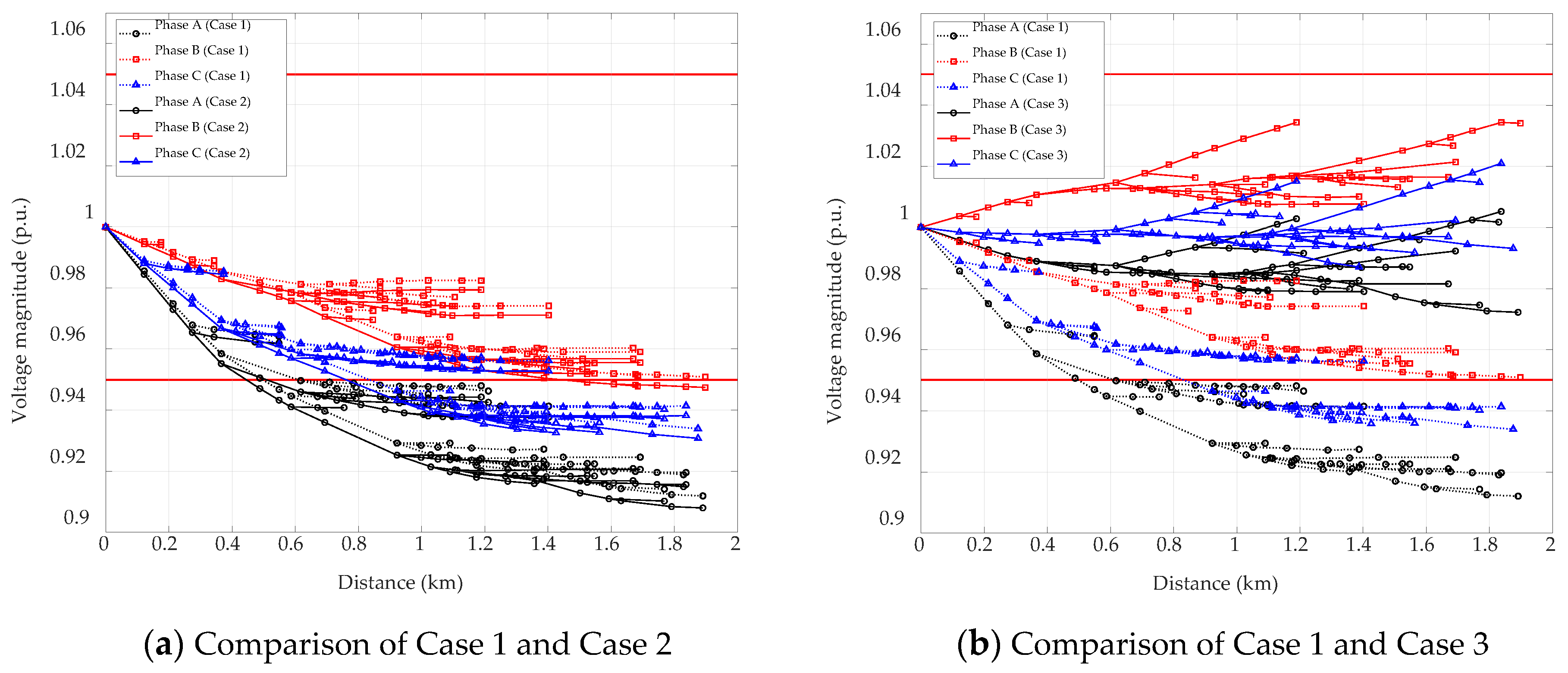
7.1. Simulation Model 1 (Case 1 to Case 3)

This simulation was conducted on the IEEE 123-bus unbalanced distribution system to evaluate the impact of distributed energy resource (DER) integration, specifically fast-charging stations for electric vehicles (FCS-EVs) and photovoltaic (PV) systems. Three cases were considered: Case 1 (base system without DERs), Case 2 (non-optimized DER deployment), and Case 3 (optimized DER deployment using improved gray wolf optimization, IGWO). The assessment focused on key performance indicators, including the voltage unbalance index $\left(VUI\right)$, voltage average $\left(V_{avg}\right)$, real and reactive power losses ($P_{loss}$ and $Q_{loss}$), and annual carbon emissions.

Table 7. Simulation Model 1: Comparison for analyzing the impact of Cases 1 to 3.

Case	${\mathit{F}}_{\mathit{b}\mathit{e}\mathit{s}\mathit{t}}$	$\mathit{V}\mathit{U}\mathit{I}$	${\mathit{V}}_{\mathit{a}\mathit{v}\mathit{g}}$	${\mathit{P}}_{\mathit{l}\mathit{o}\mathit{s}\mathit{s}}$	${\mathit{Q}}_{\mathit{l}\mathit{o}\mathit{s}\mathit{s}}$	CO2	FCS-EVs		PV Size (kVA)
		(%)	(kV)	(kW)	(kVar)	(tCO2/Y)	Bus	Size (kW)	Bus 195	Bus 251	Bus 451
1	-	4.850	2.295	109.118	218.429	-	-	-	-	-	-
2	3.212	5.202	2.287	125.600	252.400	158	149, 135, 152, 160, 197	300, 125, 200, 50, 22	-	-	-
3	1.423	3.358	2.408	57.670	113.740	−8632	-	-	1333	1356	480

presents the simulation results of Model 1 under three scenarios (Case 1 to Case 3), evaluating the impact of different DER deployment strategies on power quality, energy loss, and carbon emissions.

In Case 1, the system operated without any DERs. The simulation yielded a $VUI$ of 4.850%, an average voltage of 2.295 kV, and power losses of 109.118 kW and 218.429 kVar. CO₂ emissions were not evaluated in this scenario, as no local generation or offsetting re-sources were integrated.

In Case 2, the IGWO algorithm was applied to determine the placement of FCS-EVs, which were installed at buses 149, 135, 152, 160, and 197 with rated capacities of 300, 125, 200, 50, and 22 kW, respectively. The results indicated a $VUI$ of 5.202% and a slight de-crease in average voltage to 2.287 kV. Real and reactive power losses increased to 125.600 kW and 252.400 kVar, respectively. Additionally, annual CO₂ emissions were estimated at 158 metric tons of CO₂, which is attributed to the added charging load without sufficient renewable generation to offset the impact.

In Case 3, the IGWO algorithm was employed to determine the optimal locations and sizes of PV systems, which were installed at buses 195, 251, and 451 with capacities of 1333 kVA, 1356 kVA, and 480 kVA, respectively. This scenario demonstrated the best overall performance. The $VUI$ was reduced to 3.358%, while the average voltage increased to 2.408 kV. Real and reactive power losses were significantly reduced to 57.670 kW and 113.740 kVar, respectively. Moreover, the system achieved a CO₂ reduction of approximately 8632 metric tons per year, reflecting the substantial environmental benefits of optimal PV integration.

Figure 8a presents the convergence profiles of the improved gray wolf optimization (IGWO) for Case 2 and Case 3 over 100 iterations. The best score of Case 2 is shown on the left vertical axis (black diamond line), while that of Case 3 is displayed on the right vertical axis (red square line). Both cases (Case 2 and 3) exhibited rapid convergence during the initial 20 and 40 iterations. However, Case 3 consistently achieved a lower final objective function value of approximately 1.423 compared to 3.212 in Case 2. This result indicates that the PV-based configuration in Case 3 is more effective in meeting the optimization criteria than the FCS-EV-based deployment in Case 2.

Figure 8b illustrates the distribution of real power losses across the IEEE 123-bus system for all three cases. The x-axis represents branch numbers, the y-axis indicates the power loss in kilowatts (kW), and the z-axis separates the cases: Case 1 (red), Case 2 (green), and Case 3 (blue). The maximum power loss is the highest in Case 1 (22.222 kW), followed by Case 2 (26.925 kW), while Case 3 demonstrates the lowest loss at 6.208 kW. The consistently shorter blue bars of Case 3 reflect a substantial reduction in branch-level losses, attributed to the optimized placement and sizing of PV systems. In contrast, the higher and greater number of power losses in Case 1 and Case 2 signify the inefficiencies associated with the absence of DERs and suboptimal DER integration, respectively.

Overall, Figure 8 confirms the superior performance of optimization-guided DER planning. Case 3 not only achieved the lowest objective function value but also minimized real power losses across the distribution network, enhancing both energy efficiency and system reliability.

Figure 9 presents a comparison of voltage profiles across all three phases for selected cases, highlighting the impact of PV integration and FCS-EV loading under different system configurations. Figure 8a compares the base case (Case 1) with Case 2, where FCS-EVs were added without PV support. The voltage profiles declined across all phases, with the most pronounced reduction observed in Phase A. This result suggests that the introduction of uncoordinated EV charging increased load imbalances and worsened voltage regulation throughout the feeder.

In contrast, Figure 9—showing Case 2, which included PV integration—shows improved voltage levels compared to the base case (Case 1). The voltage drops along the feeder were less severe, especially in all phases, indicating that PV generation contributed to enhanced local voltage support.

Overall, the results in Figure 9 confirm that PV integration improved voltage stability, while FCS-EV loading without appropriate control measures resulted in greater voltage deviations and reduced power quality.

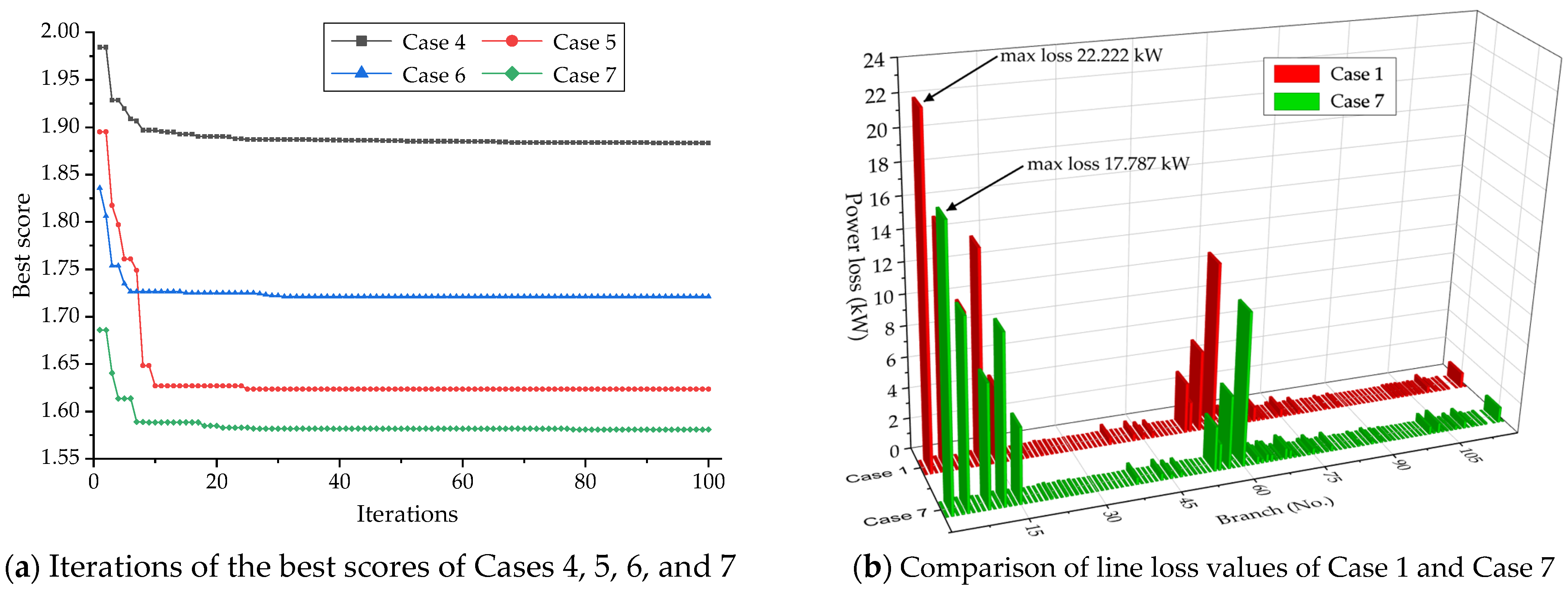
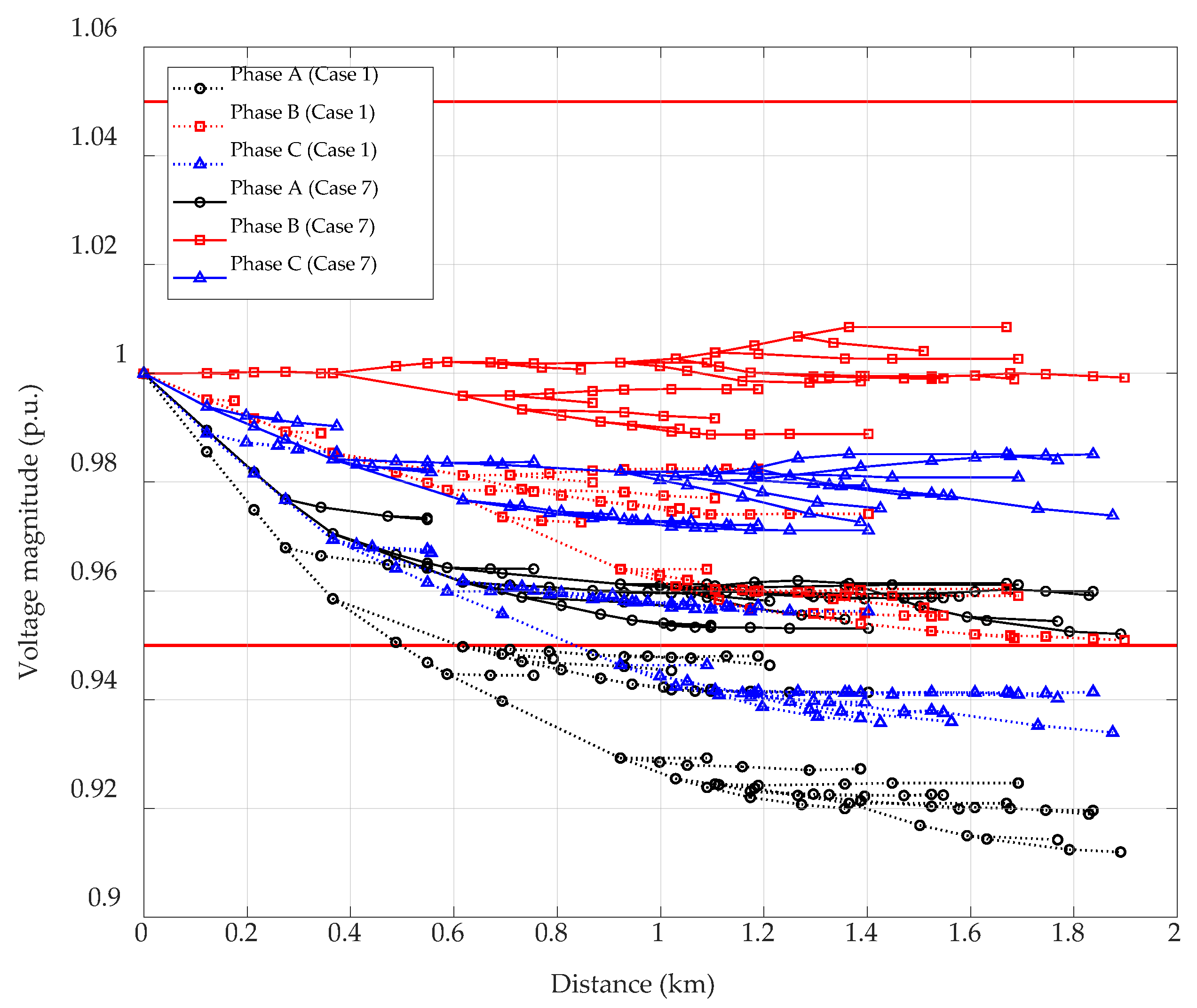
7.2. Simulation Model 2 (Case 4 to Case 7)

This section presents the results of Simulation Model 2, which examines the effects of two capacitor control strategies—balanced static var generator (BSVG) and balanced step capacitor (BSC)—on capacitor placement and sizing within a distribution power system.

Four scenarios were evaluated: Case 4 (BSVG in zone Z), Case 5 (BSVG in zone AZ), Case 6 (BSC in zone Z), and Case 7 (BSC in zone AZ).

The analysis focused on performance indicators, including the voltage unbalance index $\left(VUI\right)$, real and reactive power losses ($P_{loss}$ and $Q_{loss}$), average voltage magnitude $\left(V_{avg}\right)$, and estimated annual CO₂ emission reductions.

The comparative results are summarized in

Table 8. Simulation Model 2 is a comparison for analyzing the impact in cases 4 to 7 (without FCS-EVs).

Case	${\mathit{F}}_{\mathit{b}\mathit{e}\mathit{s}\mathit{t}}$	$\mathit{V}\mathit{U}\mathit{I}$	${\mathit{V}}_{\mathit{a}\mathit{v}\mathit{g}}$	${\mathit{P}}_{\mathit{l}\mathit{o}\mathit{s}\mathit{s}}$	${\mathit{Q}}_{\mathit{l}\mathit{o}\mathit{s}\mathit{s}}$	CO2	Capacitors
		(%)	(kV)	(kW)	(kVar)	(tCO2/Y)	Bus	Size (kVar)
4	1.883	3.679	2.336	89.958	180.610	−184	13, 135, 60, 97, 108	300, 265, 300, 300, 300
5	1.624	2.998	2.348	94.903	190.820	−136	300, 100, 105, 108, 95	295, 275, 297, 296, 300
6	1.721	3.292	2.348	90.799	182.650	−176	13, 135, 60, 97, 108	225, 125, 450, 450, 450
7	1.581	3.357	2.359	95.071	191.610	−135	105, 91, 108, 72, 62	450, 375, 450, 125, 375

. In addition, Figure 9 illustrates the convergence trends and system losses, while Figure 10 provides a voltage profile comparison between the base case (Case 1) and the best-performing case (Case 7).

Table 8 presents a comparison of the performance results of Cases 4 to 7 under Simulation Model 2. Each case was evaluated based on key indicators, including the optimization objective value $\left(Fbest\right)$, voltage unbalance index $\left(VUI\right)$, real power loss $\left(P_{loss}\right)$, reactive power loss $\left(P_{loss}\right)$, average voltage magnitude ${(V}_{avg})$, estimated annual CO₂ reduction, and the placement and size of capacitors.

Case 4, in which BSVG control was applied in zone Z, resulted in the highest voltage unbalance index (3.679%) among all cases. The real power loss was 89.958 kW, and the reactive power loss was 180.610 kVar. Despite these losses, Case 4 achieved the greatest annual CO₂ reduction, estimated at 184 tons. The capacitors were uniformly sized at 300 kVar and installed at five key locations: buses 13, 135, 60, 97, and 108. The optimization objective value $\left(Fbest\right)$ was recorded at 1.663. These results indicated that uniform capacitor sizing in limited zones could support environmental targets but may result in higher voltage imbalance.

In Case 5, the IGWO algorithm was used to determine the placement and sizing of capacitors, which were installed at buses 300, 100, 105, 108, and 95 with rated capacities of 295, 275, 297, 296, and 300 kVar, respectively. The simulation produced a voltage unbalance index $\left(VUI\right)$ of 2.998% and a slight increase in average voltage to 2.348 kV. The real power loss was reduced to 94.903 kW, and the reactive power loss decreased to 190.820 kVar. The estimated annual reduction in CO₂ emissions was approximately 136 metric tons. These results reflected the effect of additional capacitor support to meet the system’s reactive power demand.

In Case 6, the improved gray wolf optimizer (IGWO) algorithm was applied to determine the optimal placement and sizing of capacitors. The capacitors were installed at buses 13, 135, 60, 97, and 108, with rated capacities of 225, 125, 450, 450, and 450 kVar, respectively.

The simulation returned to a voltage unbalance index $\left(VUI\right)$ of 3.292% and an average voltage of 2.348 kV. The real and reactive power losses were reduced to 90.799 kW and 182.650 kVar, respectively. The estimated annual reduction in CO₂ emissions was approximately 176 metric tons. These results indicated that the use of varied capacitor sizes at strategic locations supported both power quality improvements and emission reductions.

In Case 7, the IGWO algorithm was used to determine the placement and sizing of capacitors, which were installed at buses 105, 91, 108, 72, and 62, with rated capacities of 450, 375, 450, 125, and 375 kVar, respectively.

The simulation produced a voltage unbalance index $\left(VUI\right)$ of 3.357% and increased the average voltage to 2.359 kV. Real and reactive power losses were reduced to 95.071 kW and 191.610 kVar, respectively. Additionally, the simulation assisted in lowering CO₂ emissions by 135 metric tons per year. This is the outcome of adding extra capacitors to satisfy the electrical system’s requirements.

Figure 10a presents the convergence profiles of the improved gray wolf optimization (IGWO) for Cases 4 to 7 over 100 iterations. The best scores of the objective function from Case 4 to Case 7 are shown on different color lines: black-box, red-circle, blue-triangle, and green-diamond lines. All four cases (Case 4 to Case 7) exhibit rapid convergence during the initial 30 iterations, and the values of the best score $\left(F_{best}\right)$ relative to individual values are as follows: 1.883, 1.624, 1.721, and 1.581, respectively. The significance of the best score values was discussed, and in evaluating the algorithm’s performance, Case 7 exhibited the lowest objective function value of this experimental simulation, which was approximately 1.581, compared to all cases. This result indicates that the configuration used to size and position the capacitor in Case 7 has the best efficiency in improving the voltage, as observed via the $V_{avg}$ value of 2.359 kV in Table 8.

Figure 10b presents the real power losses of the transmission lines across the IEEE 123-bus system for Cases 1 and 7, and the lowest value of the best solutions was revealed in Case 7. Thus, a comparison of the line loss values of Case 1 and Case 7 was carried out. The maximum power loss of the root line is the highest in Case 1 (22.222 kW), while Case 7 demonstrates the lowest loss at 17.787 kW. The consistently shorter blue bars of Case 7 reflect a reduction in branch-level losses, which is attributed to the optimized placement and sizing of capacitor systems.

Figure 11 presents a comparison of voltage profiles across all three phases for selected cases, highlighting the impact of capacitor installations under different system configurations. Case 7, which included capacitor installations, exhibited improved voltage levels compared to Case 1 (without a capacitor). The voltage drops along the feeder were less severe, especially in all phases, indicating that optimal capacitor placement contributed to improving the voltage magnitude profiles.

In particular, the results shown in Figure 10 strengthen the fact that optimal capacitor placement installations improved voltage magnitude profiles, which resulted in reduced voltage deviations, and this improved the voltage magnitude profiles level over 0.95 p.u.

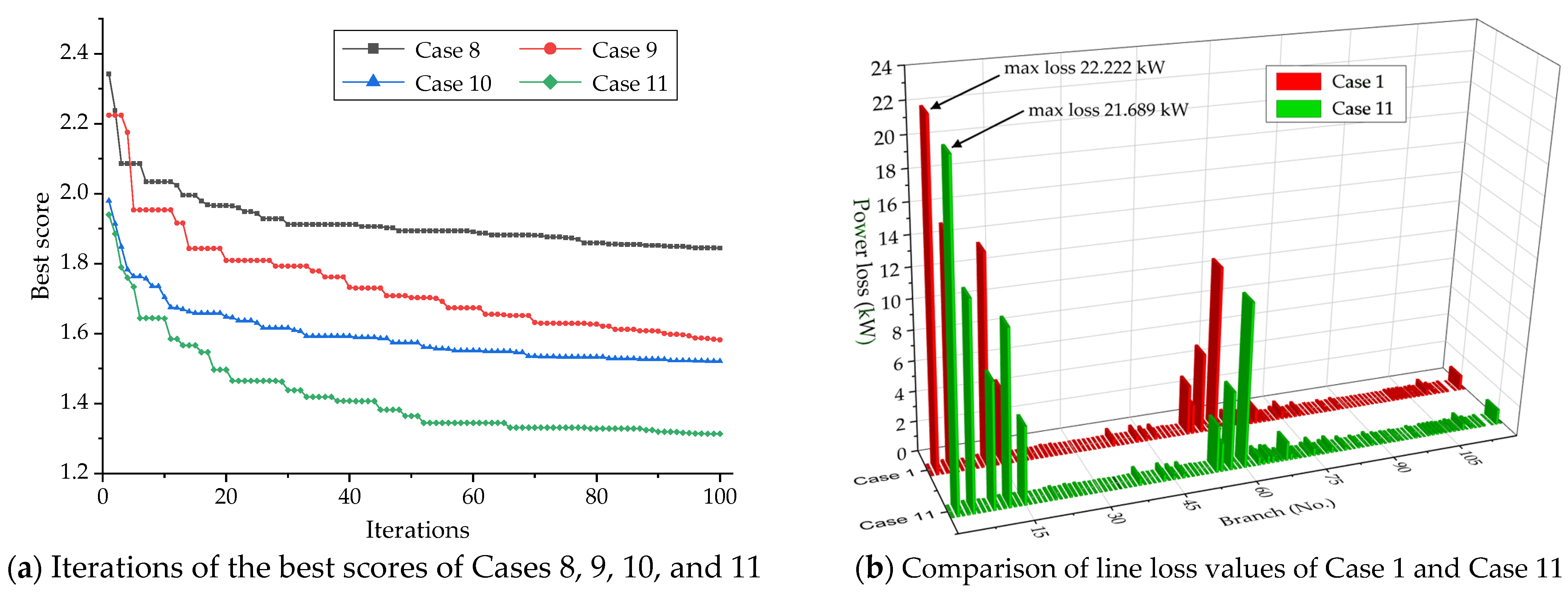
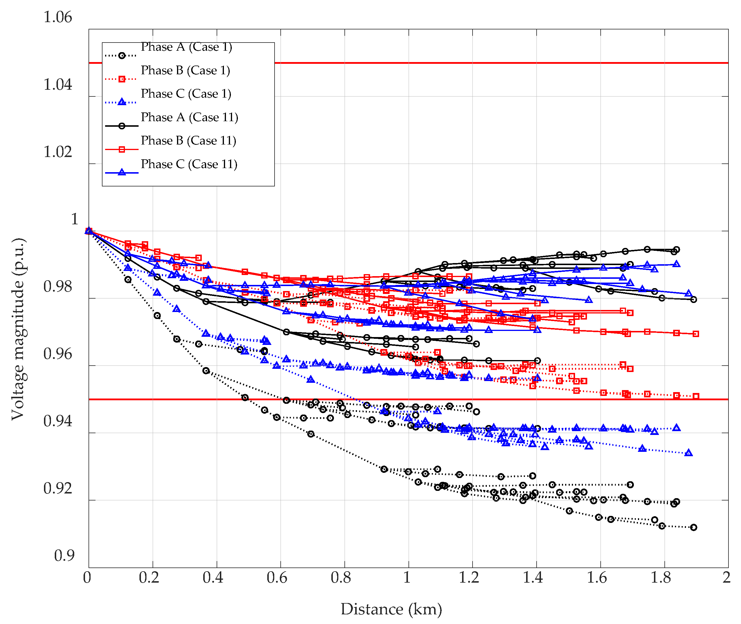
7.3. Simulation Model 3 (Case 8 to Case 11)

This scenario is integrated by FCS-EVs, representing the impact of FCS-EV’s domination over the grid. Therefore, impact moderation can be defined by implementing unbalanced static var generators (USVGs) and unbalanced step capacitor (USC) control strategies to determine the optimal sizing and locations of capacitors within the distribution power system. Four case studies were considered—Case 8 (USVG-controlled testing in Z), Case 9 (USVG-controlled testing in AZ), Case 10 (USC-controlled testing in Z), and Case 11 (USC-controlled testing in AZ)—focusing on an assessment of key performance indicators. The comparative analysis of Simulation Model 3 is summarized in

Table 9. Simulation 3: comparison to analyze impacts in Cases 8 to 11 (with FCS-EVs).

Case	${\mathit{F}}_{\mathit{b}\mathit{e}\mathit{s}\mathit{t}}$	$\mathit{V}\mathit{U}\mathit{I}$	${\mathit{V}}_{\mathit{a}\mathit{v}\mathit{g}}$	${\mathit{P}}_{\mathit{l}\mathit{o}\mathit{s}\mathit{s}}$	${\mathit{Q}}_{\mathit{l}\mathit{o}\mathit{s}\mathit{s}}$	CO2	Capacitor		FCS-EVs
		(%)	(kV)	(kW)	(kVar)	(tCO2/Y)	Bus	Size (kVar)A-B-C	Bus	Size (kW)
8	1.844	3.357	2.328	104.900	210.280	−40	29	98-99-100	149	300
							47	100-97-99	135	200
							63	100-9-99	152	50
							91	100-83-99	160	22
							300	100-92-98	197	125
9	1.583	2.763	2.341	99.962	200.440	−88	82	100-84-85	149	300
							77	100-99-96	28	22
							108	100-59-91	1	200
							89	100-82-92	7	125
							78	99-91-95	152	50
10	1.521	2.448	2.349	103.380	206.530	−55	25	150-125-150	149	300
							47	150-100-150	135	200
							64	150-125-150	152	125
							93	150-150-150	160	22
							108	150-25-150	101	50
11	1.314	1.962	2.360	103.970	207.900	−49	80	150-125-150	149	300
							72	150-50-125	30	22
							98	150-125-150	7	125
							93	150-75-125	152	50
							108	150-50-125	1	200

. The convergence characteristics and transmission line losses are illustrated in Figure 12, while the voltage magnitude profile comparison between Case 1 (the base case) and Case 11 (the best-performing scenario) is presented in Figure 13.

Table 9 shows the simulation results of Model 3 under four scenarios (Case 8 to Case 11) by evaluating the impact of FCS-EVs using reactive power compensation with different SVG and capacitor placements.

In Case 8, the IGWO algorithm was applied to determine the placement of capacitors, which were installed at buses 29, 47, 63, 91, and 300 with rated capacities per A-B-C phase of 98-99-100, 100-97-99, 100-9-99, 100-83-99, and 100-92-98 kVar, respectively. The placement of FCS-EVs was determined, and they were installed at buses 149, 135, 152, 160, and 197 with rated capacities of 300, 200, 50, 22, and 125 kW, respectively. The results show that the highest value of $F_{best}$ was greater than each case, reflecting the impact of $VUI$, $P_{loss}$, and $Q_{loss}$ with values of 1.844, 3.357%, 104.900 kW, and 210.280 kVar, respectively. Additionally, CO₂ emissions could be lowered by approximately 40 metric tons per year. This is the result of the addition of special capacitors to meet the requirements of electrical systems with FCS-EVs that are also connected to the system.

In Case 9, the IGWO algorithm was applied to determine the placement of capacitors, which were installed at buses 82, 77, 108, 89, and 78 with rated capacities per A-B-C phase of 100-84-85, 100-99-96, 100-59-91, 100-82-92, and 99-91-95 kVar, respectively. The placement of FCS-EVs was determined, and they were installed at buses 149, 28, 1, 7, and 152 with rated capacities of 300, 22, 200, 125, and 50 kW, respectively. The $F_{best}$ value of 1.583 was not the lowest of each case, but this was also revealed by minimizing the active power and reactive power loss and reducing the CO₂ by 99.962 kW, 200.440 kVar, and 88 metric tons per year.

In Case 10, the IGWO algorithm was applied to determine the placement of capacitors, which were installed at buses 25, 47, 64, 93, and 108 with rated capacities per A-B-C phase of 150-125-150, 150-100-150, 150-125-150, 150-150-150, and 150-25-150 kVar, respectively. The placement of FCS-EVs was determined, and they were installed at buses 149, 135, 152, 160, and 101 with rated capacities of 300, 200, 125, 22, and 50 kW, respectively. The $F_{best}$ value and percentage of $VUI$ of Case 10 shows that the minimized value is comparable to the Case 8 and Case 9 values of 1.521 and 2.448%. Simultaneously, Model 3 (Case 8, 9, 10, and 11) is not the best, and it can assist in lowering CO₂ emissions by about 55 metric tons per year.

In Case 11, the IGWO algorithm was applied to determine the placement of capacitors, which were installed at buses 80, 72, 98, 93, and 108 with rated capacities per A-B-C phase of 150-125-150, 150-50-125, 150-125-150, 150-75-125, and 150-50-125 kVar, respectively. The placement of FCS-EVs was determined, and they were installed at buses 149, 30, 7, 152, and 1 with rated capacities of 300, 22, 125, 50, and 200 kW, respectively. The results revealed the lowest $F_{best}$ and percentage values of $VUI$ and $V_{avg}$: 1.314, 1.962%, and 2.360 kV, respectively. Simultaneously, the maximum values were observed with respect to the active and reactive power loss and reduction in CO₂ emissions: 103.970 kW, 207.900 kVar, and 49 metric tons per year.

Figure 12a presents the convergence profiles of the improved gray wolf optimization (IGWO) for Cases 8 to 11 over 100 iterations. The best scores from Case 8 to Case 11 are shown on different color lines: the black-box, red-circle, blue-triangle, and green-diamond lines. All four cases exhibit rapid convergence during the initial 90 iterations, and the values of the best scores $\left(F_{best}\right)$ from Case 8 to Case 11 are as follows: 1.844, 1.583, 1.521, and 1.314. However, Case 11 had the lowest objective function value of this experimental simulation at approximately 1.314 compared to all cases. This result indicates that the configuration used to size and position the capacitor in Case 11 has the best efficiency in improving voltages, as observed in the $V_{avg}$ value of 2.360 kV.

Figure 12b presents the real power losses of the transmission line across the IEEE 123-bus system for both cases. A comparison of the line loss values of Case 1 and Case 11 (the best case) was carried out. The maximum power loss is the highest in Case 1 (22.222 kW), while Case 11 demonstrates the lowest loss at 21.689 kW under testing conditions. The consistently shorter green bars of Case 11 reflect a reduction in branch-level losses, which is attributed to the optimized placement and sizing of capacitors and FCS-EVs in the systems.

Figure 13 presents a comparison of voltage profiles across all three phases to select the best case, highlighting the impact of capacitor installations under different system configurations. Case 11, which included capacitor and FCS-EV installations, exhibited improved voltage levels compared to Case 1. The voltage drops along the feeder were significantly reduced across all phases, showing that the best placement of capacitors and FCS-EV installations helped improve the voltage levels in the electrical power system. In particular, the results in Figure 13 confirm that optimal capacitor placement and optimal FCS-EV installations can improve voltage stability, which results in reduced voltage deviations and greater voltage magnitude profiles.

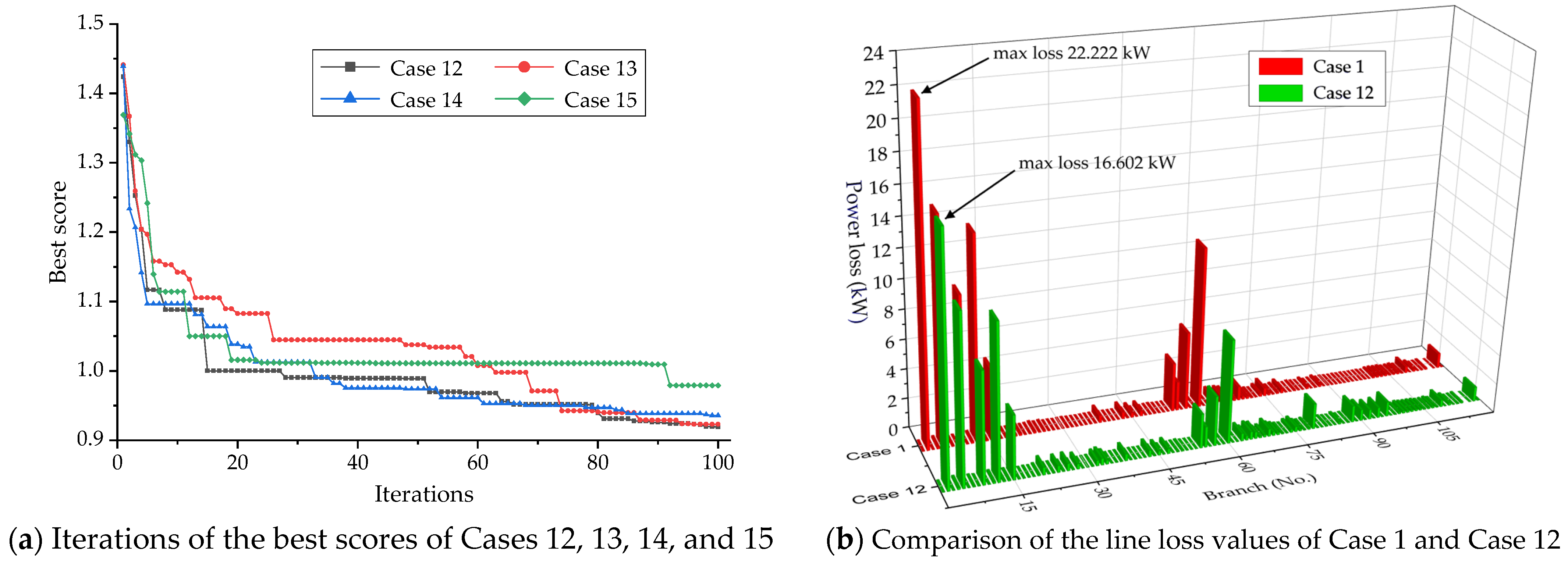
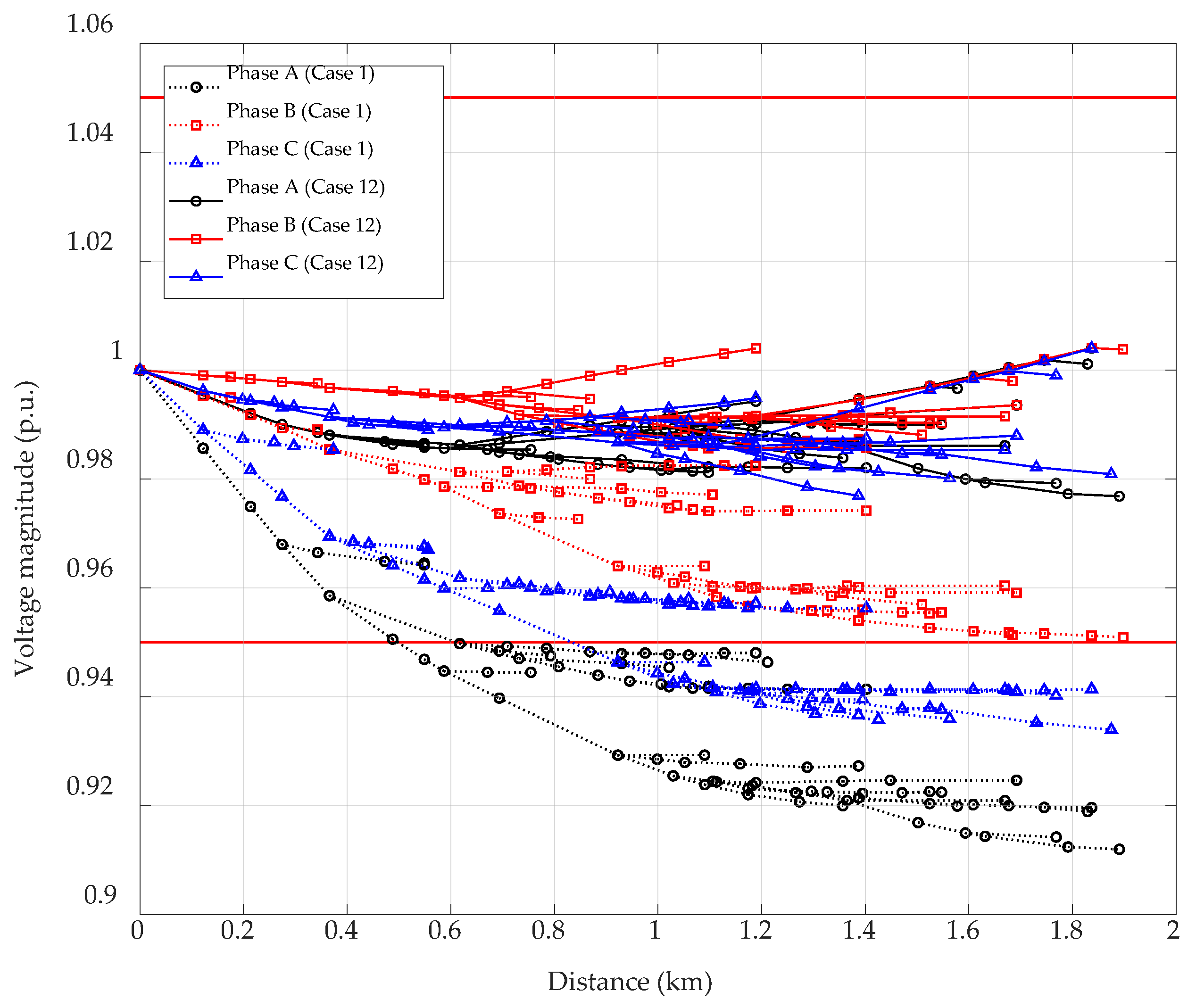
7.4. Simulation 4 Model 4 (Case 12 to Case 15)

This section presents the results of Simulation Model 4, which examined the impact of FCS-EVs in different possible system locations. Static var generator (SVG) and step capacitor (SC) control strategies were used to improve this problem. Simultaneously, a suitable PV size will be installed at fixed buses such as 195, 251, and 451 with a three-phase balanced system. Four case studies were considered—Case 12 (USVG-controlled testing in zone Z), Case 13 (USVG-controlled testing in zone AZ), Case 14 (USC-controlled testing in zone Z), and Case 15 (USC-controlled testing in all zones, AZ)—this was carried out by considering the assessment focused on key performance indicators. The comparative analysis of Simulation Model 4 is summarized in

Table 10. Simulation 4: comparison to analyze impacts in Cases 12 to 15.

Case	${\mathit{F}}_{\mathit{b}\mathit{e}\mathit{s}\mathit{t}}$	$\mathit{V}\mathit{U}\mathit{I}$	${\mathit{V}}_{\mathit{a}\mathit{v}\mathit{g}}$	${\mathit{P}}_{\mathit{l}\mathit{o}\mathit{s}\mathit{s}}$	${\mathit{Q}}_{\mathit{l}\mathit{o}\mathit{s}\mathit{s}}$	CO2	Capacitor		FCS-EV		PV Size (kVA)
		(%)	(kV)	(kW)	(kVar)	(tCO2/Y)	Pos.	Size (kVar) A-B-C	Pos.	Size (kW)	Pos. 195	Pos. 251	Pos. 451
12	0.919	1.376	2.383	90.366	179.53	−5602	28	75-6-70	149	200	1242	623	246
							49	96-6-92	48	50
							62	90-12-63	54	125
							97	89-15-38	95	300
							197	52-8-32	105	22
13	0.932	1.41	2.383	87.368	171.97	−5992	63	59-18-81	95	300	1374	549	329
							135	95-9-85	93	200
							62	87-7-13	35	50
							49	88-9-66	23	22
							66	100-11-50	53	125
14	0.936	1.063	2.384	120.05	240.34	−4688	25	125-25-125	149	300	745	558	563
							40	150-25-100	135	125
							55	75-25-50	52	200
							67	100-25-100	100	22
							108	125-25-75	197	50
15	0.979	1.297	2.391	118.75	238.92	−4734	50	50-25-75	135	50	715	365	799
							80	125-25-125	152	125
							35	100-25-25	149	200
							81	125-50-75	1	300
							49	125-50-12	40	22

. The convergence characteristics and transmission line losses are illustrated in Figure 14, while the voltage magnitude comparison between Case 1 (the base case) and Case 12 (the best-performance scenario) is presented in Figure 15.

Table 10 shows the simulation results of Model 4 under four scenarios (Case 12 to Case 15) by evaluating the impact of FCS-EVs using reactive power compensation with different SVG and capacitor placements. Simultaneously, the PVs are installed by using three phases in a balanced system.

In Case 12, the IGWO algorithm was applied to determine the placement of capacitors, which were installed at buses 28, 49, 62, 97, and 197 with rated capacities per A-B-C phase of 75-6-70, 96-6-92, 90-12-63, 89-15-38, and 52-8-32 kVar, respectively. The placement of FCS-EVs was determined, and they were installed at buses 149, 48, 54, 95, and 105 with rated capacities of 200, 50, 125, 300, and 22 kW, respectively. The placement of PV3P was determined, and it was installed with rated capacities of 1242, 623, and 246 kVA. The results indicated that the lowest $F_{best}$ value was 0.919. This is the best outcome of Model 4 (Cases 12, 13, 14, and 15), but it does not represent the best objective function values. However, $VUI$, $V_{avg}$, $P_{loss}$, $Q_{loss}$, and CO₂-emission-lowering values were 1.376%, 2.383 kV, 90.366 kW, 179.530 kVar, and 5602 metric tons per year, respectively. While Case 12 may not produce noticeable results, overall, it still represents the best outcome of Model 4. This is the result of the addition of special capacitors and PVs relative to meeting the requirements of electrical systems with FCS-EVs.

In Case 13, the IGWO algorithm was applied to determine the placement of capacitors, which were installed at buses 63, 135, 62, 49, and 66 with rated capacities per A-B-C phase of 59-18-81, 95-9-85, 87-7-13, 88-9-66, and 100-11-50 kVar, respectively. The placement of FCS-EVs was determined, and they were installed at buses 95, 93, 35, 23, and 53 with rated capacities of 300, 200, 50, 22, and 125 kW, respectively. The placement of PV3Ps was also determined, and they were installed with rated capacities of 1374, 549, and 329 kVA. The results show that the lowest values of $P_{loss}$ and $Q_{loss}$ were 87.368 kW and 171.970 kVar, respectively. CO₂ emissions were also lowered by approximately 5992 metric tons per year. Moreover, the maximum value of the $VUI$ was 1.410%.

In Case 14, the IGWO algorithm was applied to determine the placement of capacitors, which were installed at buses 25, 40, 55, 67, and 108 with rated capacities per A-B-C phase of 125-25-125, 150-25-100, 75-25-50, 100-25-100, and 125-25-75 kVar, respectively. The placement of FCS-EVs was determined, and they were installed at buses 149, 135, 52, 100, and 197 with rated capacities of 300, 125, 200, 22, and 50 kW, respectively. The placement of PV3Ps was determined, and they were installed with rated capacities of 745, 558, and 563 kVA. The $F_{best}$ value was 0.936, and this was not the lowest of each case; however, these results are revealed by minimizing the $VUI$ of 1.063%. Simultaneously, the maximum values of $P_{loss}$ and $Q_{loss}$ were 120.050 kW and 240.340 kVar, respectively. Additionally, CO₂ emissions were lowered by approximately 4688 metric tons per year.

In Case 15, the IGWO algorithm was applied to determine the placement of capacitors, which were installed at buses 50, 80, 35, 81, and 49 with rated capacities per A-B-C phase of 50-25-75, 125-25-125, 100-25-25, 125-50-75, and 125-50-125 kVar, respectively. The placement of FCS-EVs was determined, and they were installed at buses 135, 152, 149, 1, and 40 with rated capacities of 50, 125, 200, 300, and 22 kW, respectively. The placement of PV3Ps was carried out, and they were installed with rated capacities of 715, 365, and 799 kVA. The results show the highest $F_{best}$ value, which was greater than in the other cases, reflecting the impact of $VUI$, $P_{loss}$, and $Q_{loss}$: 0.979, 1.297%, 118.750 kW, and 238.920 kVar, respectively. Additionally, CO₂ emissions were lowered by approximately 4734 metric tons per year.

Figure 14a presents the convergence profiles of the improved gray wolf optimization (IGWO) for Case 12 to Case 15 over 100 iterations. The best scores from Case 12 to Case 15 are shown using colored lines: the black-box, red-circle, blue-triangle, and green-diamond lines. All four cases exhibit rapid convergence during the initial 90 iterations, for which the values of the best scores $\left(F_{best}\right)$ from Case 12 to Case 15 are as follows: 0.919, 0.932, 0.936, and 0.979, respectively. However, Case 12 exhibited the lowest objective function value of this experimental simulation at approximately 0.919 compared to all cases. This result indicates that the configuration used to size and position the capacitor in Case 11 has the best efficiency in improving the voltage magnitude profiles of the electrical power system.

Figure 14b presents the active power losses of the transmission line across the IEEE 123-bus system for both cases and the comparison of line loss values for Cases 1 and 12. The maximum power loss is the highest in Case 1 (22.222 kW), while Case 12 demonstrates the lowest loss at 16.602 kW. The consistently shorter green bars of Case 12 reflect a reduction in branch-level losses, which is attributed to the optimized placement and sizing of capacitors, FCS-EV, and PV3P in systems.

Figure 15 shows a comparison of voltage levels in all three phases for different cases, emphasizing how capacitor installations affect the system in various setups. Case 12, which had capacitor, FCS-EV, and PV3P installations, exhibited better voltage levels than Case 1. The voltage drops along the feeder were not as severe, especially in all phases, suggesting that the best capacitor, FCS-EV, and PV3P placements helped improve the voltage levels of the grid. Case 12, which included capacitor, FCS-EV, and PV3P installations, exhibited improved voltage levels compared to Case 1. The voltage drops along the feeder were lower, especially in all phases, showing that the best capacitor, FCS-EV, and PV3P placements helped improve the voltage levels of the grid (Figure 15). The results revealed that the best capacitor placement and FCS-EV and PV3P installations enhanced voltage stability, resulting in lower voltage deviations and improved power quality.

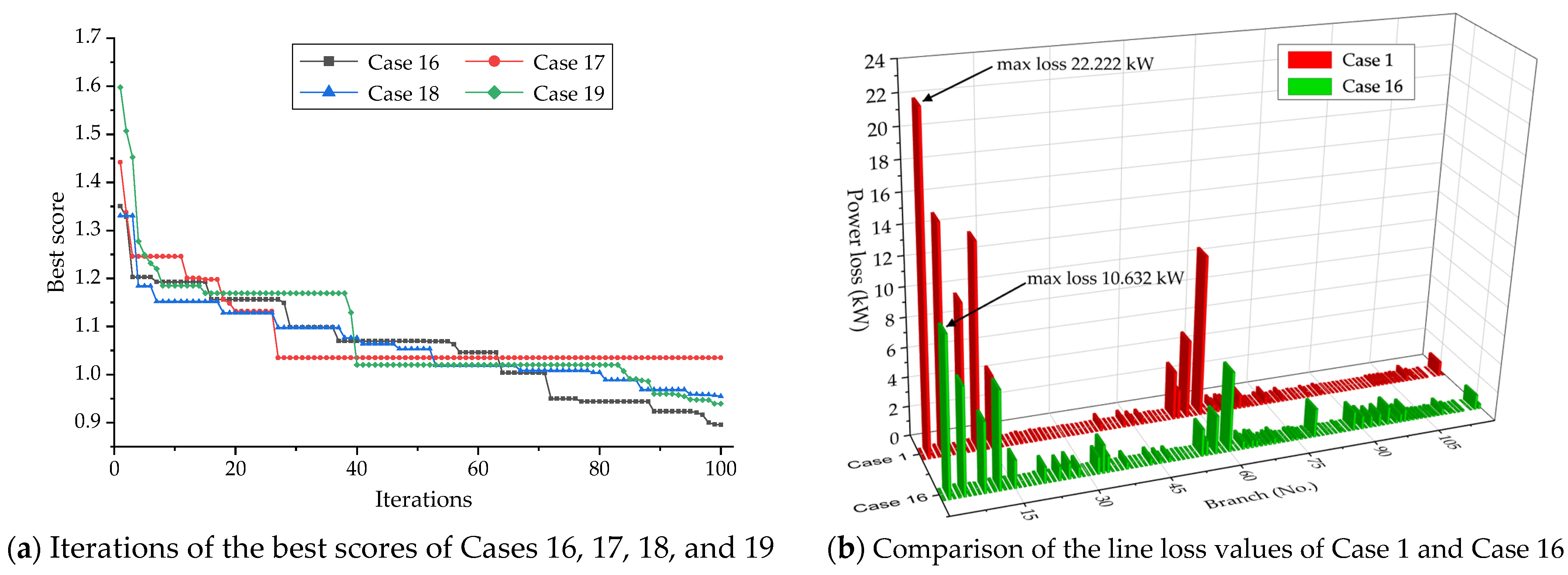
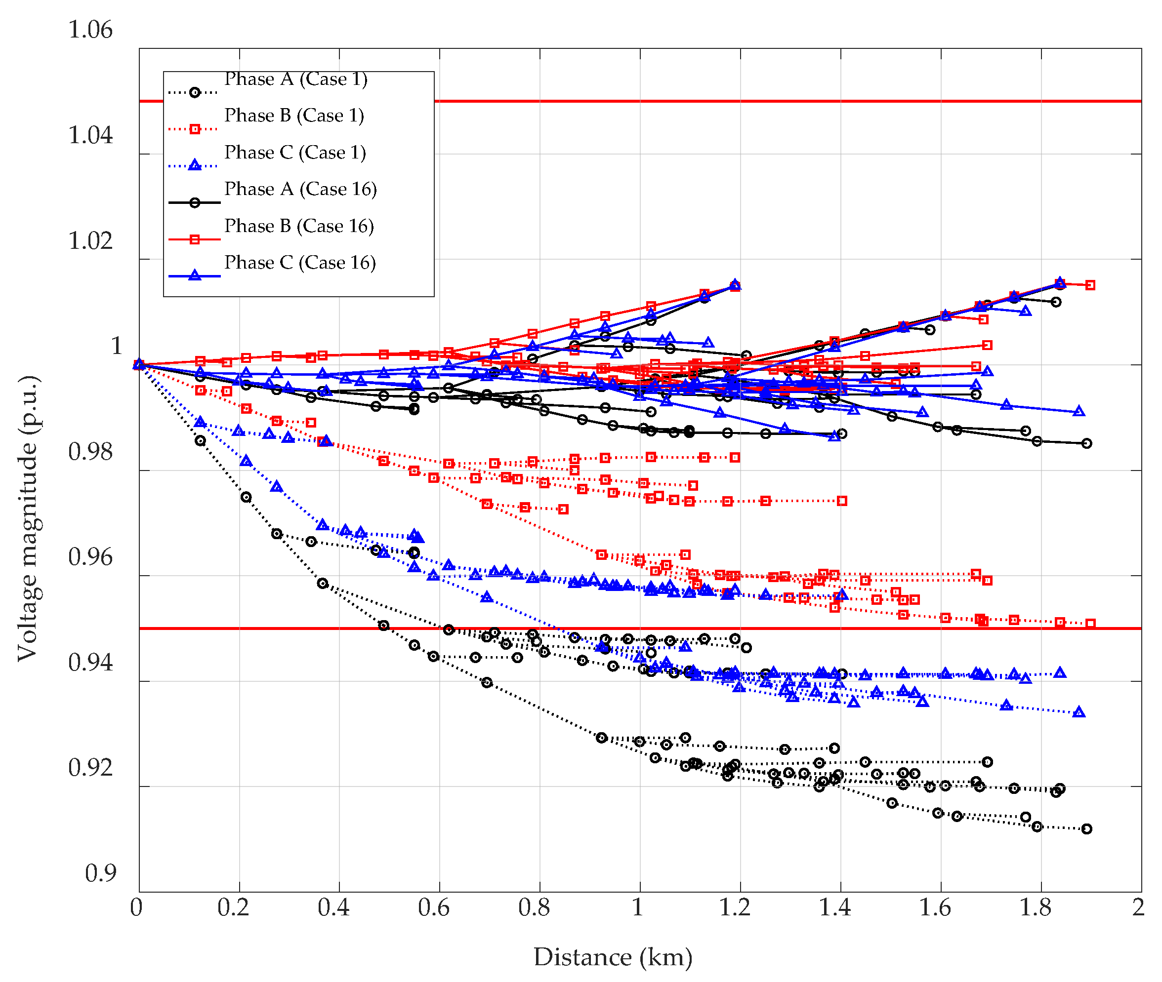
7.5. Simulation 5 Model 5 (Case 16 to Case 19)

Simulation 5 was carried out to find the optimal conditions for implementing unbalanced static var generator (USVG) and unbalanced step capacitor (USC) control. The optimization techniques applied strategies for determining the optimal sizing and positions of capacitors and FCS-EV and the most suitable sizing per phase of PV1P-installed positions at buses 195, 251, and 451 within the distribution power system.

Four case studies were considered—Case 16 (USVG-controlled testing in zone Z), Case 17 (USVG-controlled testing in zone AZ), Case 18 (USC-controlled testing in zone Z), and Case 19 (USC-controlled testing in zone AZ)—and the assessment focused on key performance indicators. The comparative analysis of Simulation Model 5 is summarized in

Table 11. Simulation Model 4: comparison for analyzing the impact in Cases 16 to 19.

Case	${\mathit{F}}_{\mathit{b}\mathit{e}\mathit{s}\mathit{t}}$	$\mathit{V}\mathit{U}\mathit{I}$	${\mathit{V}}_{\mathit{a}\mathit{v}\mathit{g}}$	${\mathit{P}}_{\mathit{l}\mathit{o}\mathit{s}\mathit{s}}$	${\mathit{Q}}_{\mathit{l}\mathit{o}\mathit{s}\mathit{s}}$	CO2	Capacitor		FCS-EV		PV Size (kVA)
		(%)	(kV)	(kW)	(kVar)	(tCO2/Y)	Pos.	Size (kVar) A-B-C	Pos.	Size (kW)	Pos.195 A-B-C	Pos.251 A-B-C	Pos.451 A-B-C
16	0.896	1.626	2.404	74.599	148.86	−3418	25	48-16-57	29	200	475-482-462	497-406-385	230-70-75
							51	6-11-15	50	22
							53	73-39-82	55	50
							450	19-69-75	95	300
							101	30-12-77	101	125
17	1.035	1.428	2.383	125.31	252.39	−2249	13	52-75-28	152	300	291-252-227	378-288-345	267-191-232
							72	40-57-93	149	22
							149	64-64-15	250	200
							135	89-40-61	1	50
							108	83-6-39	47	125
18	0.955	1.067	2.39	134.08	270.09	−1926	18	25-50-125	7	200	257-223-230	357-209-276	22-192-253
							47	100-50-75	42	125
							55	75-50-125	52	300
							76	75-75-75	78	22
							108	150-50-50	101	50
19	0.94	1.309	2.385	122.78	246.69	−1598	66	50-75-50	14,940	300	209-239-220	280-65-262	148-121-218
							51	125-50-75	99	50
							97	125-125-75	25	125
							108	150-50-75	81	200
							48	50-50-100	14,940	22

. The convergence characteristics and transmission line losses are illustrated in Figure 16, while the voltage magnitude profile comparison between Case 1 (the base case) and Case 16 (the best-performance scenario) is presented in Figure 17.

Table 11 shows the simulation results of Model 5 under four scenarios (Case 16 to Case 19) by evaluating the impact of PV1P (fixed position) using active power compensation with different SVG and capacitor placements.

In Case 16, the IGWO algorithm was applied to determine the placement of capacitors, which were installed at buses 25, 51, 53, 450, and 101 with rated capacities per A-B-C phase of 48-16-57, 6-11-15, 73-39-82, 19-69-75, and 30-12-77 kVar, respectively. The placement of FCS-EVs was determined, and they were installed at buses 29, 50, 55, 95, and 101 with rated capacities of 200, 22, 50, 300, and 125 kW, respectively. The placement of PV1Ps was also determined, and they were installed at fixed buses 195, 251, and 451 with rated capacities per phase of 475-482-462, 497-406-385, and 230-70-75 kVA, respectively. The results revealed the lowest $F_{best}$, active power $P_{loss}$, and reactive power $Q_{loss}$ values of 0.896, 74.599 kW, and 148.680 kVar, respectively. Simultaneously, the maximum $V_{avg}$ and CO₂ reduction values were 2.404 kV and approximately 3418 metric tons per year. These are the best values of Model 5 (Cases 16, 17, 18, and 19). Case 16 achieved the lowest objective function value ($F_{best}$ = 0.896) due to its use of unbalanced capacitors and static var generators (SVGs) under a distributed control (DC) strategy in the simulated system. This approach allows for the more precise adjustment of reactive power compared to other methods, particularly under unbalanced load conditions. With only 630.136 kVar of installed capacity and the lowest total cost of USD 9041, Case 16 demonstrated the most efficient and well-balanced performance within our optimization framework.

In Case 17, the IGWO algorithm was applied to determine the placement of capacitors, which were installed at buses 13, 72, 149, 135, and 108 with rated capacities per A-B-C phase of 52-75-28, 40-57-93, 64-64-15, 89-40-61, and 8-36-39 kVar, respectively. The placement of FCS-EVs was determined, and they were installed at buses 152, 149, 250, 1, and 47 with rated capacities of 300, 22, 200, 50, and 125 kW, respectively. The placement of PV1Ps was determined, and they were installed at fixed buses 195, 251, and 451 with rated capacities per phase of 291-252-227, 378-288-345, and 267-191-232 kVA, respectively. The results show the highest $F_{best}$ value compared to the other cases; moreover, the $VUI$, $P_{loss}$, and $P_{loss}$ values were 1.035, 1.428%, 125.310 kW, and 252.390 kVar, respectively. Additionally, CO₂ emissions were lowered by approximately 2249 metric tons per year.

In Case 18, the IGWO algorithm was applied to determine the placement of capacitors, which were installed at buses 18, 17, 55, 76, and 108 with rated capacities per A-B-C phase of 25-50-125, 100-50-75, 75-50-125, 75-75-75, and 150-50-50 kVar, respectively. The placement of FCS-EVs was determined, and they were installed at buses 7, 42, 52, 78, and 101 with rated capacities of 200, 125, 300, 22, and 50 kW, respectively. The placement of PV1Ps was determined, and they were installed at fixed buses 195, 251, and 451 with rated capacities per phase of 257-223-230, 357-209-276, and 22-192-253 kVA, respectively. The $F_{best}$ value of 0.955 was not the lowest for each case; $VUI$ minimization and CO₂-emission-lowering values were 1.067 kW and 1926 metric tons per year.

In Case 19, the IGWO algorithm was applied to determine the placement of capacitors, which were installed at buses 66, 51, 97, 108, and 48 with rated capacities per A-B-C phase of 50-75-50, 125-50-75, 125-125-75, 150-50-75, and 50-50-100 kVar, respectively. The placement of FCS-EVs was determined, and they were installed at buses 149, 40, 99, 25, and 81 with rated capacities of 300, 50, 125, 200, and 22 kW, respectively. The placement of PV1Ps was determined, and they were installed at fixed buses 195, 251, and 451 with rated capacities per phase of 209-239-220, 280-65-262, and 148-121-218 kVA, respectively. The $F_{best}$ of Case 19 exhibits a lower value compared to Case 17 and Case 18: 0.940, 1.035, and 0.955, respectively. Additionally, CO₂ emissions are lowered by approximately 1598 metric tons per year.

Figure 16a presents the convergence profiles of the improved gray wolf optimization (IGWO) for Case 16 to Case 19 over 100 iterations. The best scores from Case 16 to Case 19 are shown in the colored lines: the black-box, red-circle, blue-triangle, and green-diamond lines. All four cases exhibit rapid convergence during the initial 100 iterations, for which the best scores $\left(F_{best}\right)$ of Case 16 to Case 19 are as follows: 0.896, 1.035, 0.955, and 0.940, respectively. However, Case 16 has the lowest objective function value of this experimental simulation at approximately 0.896, compared to all cases. This result indicates that the configuration used to size and position the capacitor in Case 16 has the best efficiency in improving voltages.

Figure 16b illustrates the actual power losses of the transmission line throughout the IEEE 123-bus system for both scenarios. A comparison of line loss values between Case 1 and Case 16 was carried out. The maximum power loss is the greatest in Case 1 (22.222 kW), while Case 12 exhibits a minimum loss of 10.632 kW. The consistently shorter green bars of Case 16 indicate a decrease in branch-level losses due to the optimized positioning and sizing of capacitors, FCS-EVs, and PV1Ps inside the systems.

Figure 17 illustrates a comparison of voltage magnitude profiles across all three phases for various scenarios, emphasizing the effect of capacitor installations under distinct system topologies. Case 16, incorporating FCS-EV and PV1P capacitor installations, shows enhanced voltage levels relative to Case 1. The voltage magnitude profiles are significantly enhanced, particularly throughout all stages, meaning that the appropriate positioning of capacitor, FCS-EV, and PV1P installations is the primary contributor to the voltage enhancement observed, which is indicated by the average voltage of 2.404 kV. The results depicted in Figure 17 demonstrate that the ideal placement of the capacitor, FCS-EV, and PV1P significantly improves voltage stability, diminishes voltage deviations, and enhances the power quality relative to voltage stability.

7.6. Comparison of Economic Analysis Results

In this section, a comparative analysis is performed on all 19 case studies to determine the installation size and cost of capacitors for voltage improvement. The economic reason is crucial for investment decision-making relative to improving the electrical power system. The cost of medium-voltage static var generators (SVGs) ranges from USD 6.82 to 13.64 per kVar depending on the voltage level, enclosure type, and cooling system [50,51]. In contrast, basic medium-voltage capacitor units cost between USD 2 and USD 10 per kVar depending on the manufacturer and specifications [52]. This research study is defined by the average value of SVGs and capacitor banks per kVar: USD 10.33 and USD 6, respectively. However, in realistic installation conditions, the actual values may be higher than the values observed here.

Table 12. Comparison of the investment costs of reactive power compensation.

Simulation Model	Case	Total Reactive Power (kVar)	Cost of Investment (USD)
1	1	-	-
	2	-	-
	3	-	-
2	4 (SVG)	1464.400	15,127.252
	5 (SVG)	1462.700	15,109.691
	6	1700.000	10,200.000
	7	1775.000	10,650.000
3	8 (SVG)	1371.700	14,169.661
	9 (SVG)	1370.600	14,158.298
	10	2025.000	12,150.000
	11	1850.000	11,100.000
4	12 (SVG)	742.080	7665.6864
	13 (SVG)	778.222	7782.220
	14	1150.000	6900.000
	15	1125.000	6750.000
5	16 (SVG)	630.136	6509.305
	17 (SVG)	806.000	10,650.000
	18	1150.000	6900.000
	19	1225.000	7350.000

shows a comparison of reactive power compensation investment costs, which are divided relative to five simulation models—the sub-components are capacitors and static var generator (SVGs). The investment costs of both capacitors and static var generator (SVGs) are presented using the total reactive power values. The maximum and minimum costs of the SVG are presented relative to Case 4 and Case 16, with costs of USD 15,127.252 and USD 6509.305, respectively. The maximum and minimum costs of the capacitors are presented relative to Case 7 and Case 15, with costs of USD 10,650.000 and USD 6750.000, respectively. Therefore, the size of the required reactive power determines the investment cost. It is interesting to note that SVG investments cost more than capacitors. Simultaneously, the total sizing of the reactive power of SVGs is less than the capacitors that resonate with the SVGs, and this can be generated by finding the reactive power values.

7.7. Discussion of Simulations

This study introduces a multi-scenario simulation framework to assess the efficacy of distributed control strategies in an imbalanced IEEE 123-bus distribution network. A total of nineteen cases, grouped into five model configurations, were developed to investigate various combinations of control components, including fast-charging-station electric vehicles (FCS-EVs), single-phase and three-phase photovoltaic systems (PV1P and PV3P), static var generators (BSVG/USVG), and step capacitors (BSC/USC), which are applied under both zone-specific and comprehensive deployment schemes. The system’s performance was evaluated using six key metrics: the optimization objective function ($F_{best}$), voltage unbalance index ($VUI$), average voltage ($V_{avg}$), active power loss ($P_{loss}$), reactive power loss ($Q_{loss}$), and CO₂ emissions.

In the comparative analysis of balanced and unbalanced capacitor and SVG configurations (Model 2 and Model 3, Cases 4 to 11, without PV integration), the average optimization objective values were 1.702 for Cases 4–7 (BSC and BSVG) and 1.566 for Cases 8–11 (USC and USVG). This indicates that the unbalanced configurations outperform their balanced counterparts. The average voltage unbalance index further supports this trend, with values of 3.332% for BSC/BSVG and 2.633% for USC/USVG. However, the integration of FCS-EVs resulted in an increase in both active and reactive power losses.

In a second comparison involving Models 4 and 5 (Cases 12 to 19), the influence of PV integration with unbalanced control components was assessed. The average objective optimization values for Model 4 (Cases 12–15: USVG + PV3P) and Model 5 (Cases 16–19: USVG + PV1P) were 0.942 and 0.957, respectively. These results suggest that three-phase PV systems (PV3P) are more effective than single-phase PV systems (PV1P) in improving overall system performance, particularly in reducing voltage imbalances and active and reactive power losses. Nonetheless, the average voltage magnitude ($V_{avg}$) of Model 4 was slightly lower than that of Model 5. Notably, Case 16 (Model 5) demonstrated that combining PV1P with USVG can effectively enhance voltage magnitudes, reduce power losses, and improve voltage unbalance conditions.

Figure 18 presented a comparative analysis of the real power loss $\left(P_{loss}\right)$, reactive power loss $\left(Q_{loss}\right)$, and objective function $\left(F_{best}\right)$ across 19 simulation cases. Among these indicators, $F_{best}$ served as the principal metric for evaluating multi-objective optimization outcomes, as it integrated the combined effects of energy losses, voltage deviations, unbalance values, and associated costs. Our analysis revealed that Case 16 obtained the lowest $F_{best}$ value, indicating the most effective system performance overall. This case incorporated a combination of voltage support compensation, electric vehicle (EV) control, and PV1P randomization applied within each zone. The observed reduction in both Ploss and $Q_{loss}$ in this case confirmed that the strategy effectively minimized energy losses while maintaining voltage quality and system balance. In contrast, Case 2 exhibited the highest $F_{best}$ value primarily due to substantial power losses and voltage imbalances resulting from uncoordinated EV integration. This outcome emphasized the adverse effects of uncontrolled EV deployment on system performance and validated the need for intelligent planning. Cases 3 and 4 showed significant improvements over the base case, with notable reductions in Ploss and $Q_{loss}$ that resulted in lower $F_{best}$ values. However, some of the later cases, such as Cases 18 and 19, demonstrated increased losses and a corresponding increase in $F_{best}$; this is likely due to the less efficient distribution of control strategies across all zones. The overall trend of $F_{best}$ values decreased steadily from Case 2 to Case 16, indicating the increasing effectiveness of the applied optimization framework. These results highlighted the importance of targeted reactive power compensation, zone-based control, and coordinated resource allocation. The findings support the use of multi-objective optimization in enhancing technical efficiency, improving voltage stability, and supporting environmentally and economically sustainable distribution system operations.

Figure 19 presents the trends in the objective function ($F_{best}$), voltage unbalance index ($VUI$), average voltage ($V_{avg}$), and CO₂ emissions across all 19 simulation cases. $F_{best}$ served as the primary performance indicator, reflecting the combined impact of energy losses, voltage imbalances, and environmental costs. $F_{best}$ decreased sharply between Case 2 and Case 3 and reached its minimum value in Case 16. This confirmed that the configuration in Case 16—which applied voltage support, controlled EV loads, and PV1P randomization—realized the most effective balance across all objectives. $VUI$ followed a similar trend, with the lowest values occurring in Cases 12 to 16, indicating improved phase voltage symmetries due to the reactive power support implemented. $V_{avg }$ remained stable across all cases, and it was consistently between 2.3 and 2.4 kV, suggesting that voltage regulation was maintained regardless of the control strategy. CO₂ emissions were significantly reduced in Case 3 and remained lower than the base case throughout all optimized scenarios. These results demonstrate that coordinated zone-based optimization effectively minimizes losses, improves voltage quality, and supports emission reduction. Case 16 offered the best overall performance, validating the use of $F_{best}$ as a reliable composite metric for guiding control strategies in modern distribution systems.

Table 13. Convergence performance of IGWO.

Model 1		Model 2		Model 3		Model 4		Model 5
Case	Iterations	Case	Iterations	Case	Iterations	Case	Iterations	Case	Iterations
2	17	4	82	8	96	12	98	16	99
3	78	5	25	9	100	13	94	17	27
		6	31	10	92	14	98	18	100
		7	78	11	94	15	92	19	99
Avg.	47.50		54.00		95.50		95.50		81.25

presents the convergence performance analysis of IGWO across five models, revealing a clear relationship between system complexity and computational requirements. Model 1, representing the baseline configuration with randomized FCS-EV and PV systems, achieved the fastest convergence at 47.50 iterations. In contrast, Model 2—with conventional capacitor control (BSVG and BSC) implemented—required slightly more iterations at 54.00. The most computationally intensive configurations were Models 3 and 4; both averaged 95.50 iterations due to unbalanced control strategies and three-phase PV system integration, respectively, demonstrating how unbalanced systems and multi-phase coordination can significantly impact optimization efficiency. Model 5—incorporating single-phase PV systems—required an intermediate number of 81.25 iterations for convergence. With an overall average of 73.67 iterations across all case studies, these results demonstrate that the system’s complexity directly influences computational requirements, providing valuable insights into the scalability and practical applicability of IGWO for diverse power system optimization scenarios.

8. Conclusions

This research study presented a hybrid objective optimization framework for unbalanced power distribution systems, addressing a key gap in conventional research, which typically assumes balanced conditions. Based on the IEEE 123-bus benchmark, nineteen simulation scenarios were constructed to evaluate different combinations of distributed energy resources (DERs), including fast-charging electric vehicles (FCS-EVs), single-phase and three-phase photovoltaic systems (PV1P and PV3P), static var generators (USVG and BSVG), and step capacitors (USC and BSC), implemented under both zone-specific and system-wide control strategies.

The improved gray wolf optimization (IGWO) algorithm was used to optimize the placement and sizing of these resources by considering multiple objectives: active and reactive power losses, voltage deviations, voltage imbalances, average voltages, and installation costs. The results consistently showed that unbalanced control strategies outperformed balanced strategies in terms of technical efficiency and environmental benefits.

Among all cases, Case 16 achieved the best performance, combining PV1P and USVG under zone-specific distributed control. This configuration yielded significant improvements in voltage regulation and lower power losses (74.599 kW and 148.86 kVar) and notable CO₂ reductions (−3418 kg/year). This study also demonstrated that control strategies evolving from fixed-step balanced capacitors to unbalanced SVGs provide increasingly precise reactive power compensation and better system stability.

Overall, the proposed framework offers a scalable and effective approach for improving power quality and operational efficiency in modern distribution networks.

Future studies will extend this framework to include adaptive control algorithms, time-series-based uncertainty modeling, and multi-period coordination. These enhancements aim to improve system performance under real-world dynamic conditions and further support the integration of smart grid technologies and electric mobility.

References

1. IEA. Electricity Market Report 2023; IEA: Paris, France, 2023. [Google Scholar]
2. Rezapour, H.; Fathnia, F.; Fiuzy, M.; Falaghi, H.; Lopes, A.M. Enhancing power quality and loss optimization in distorted distribution networks utilizing capacitors and active power filters: A simultaneous approach. Int. J. Electr. Power Energy Syst. 2024, 155, 109590. [Google Scholar] [CrossRef]
3. Poshtyafteh, M.; Barati, H.; Falehi, A.D. Optimal placement of distribution network-connected microgrids on multi-objective energy management with uncertainty using the modified Harris Hawk optimization algorithm. IET Gener. Transm. Distrib. 2024, 18, 809–833. [Google Scholar] [CrossRef]
4. Pamuk, N.; Uzun, U.E. Optimal Allocation of Distributed Generations and Capacitor Banks in Distribution Systems Using Arithmetic Optimization Algorithm. Appl. Sci. 2024, 14, 831. [Google Scholar] [CrossRef]
5. Mohanad Muneer, Y.; Ali Nasser, H.; Wathiq Rafa, A.; Daniel Augusto, P. Power Loss Reduction and Reliability Improvement of Radial Distribution Systems Using Optimal Capacitor Placement Technique. J. Technol. 2024, 6, 1–9. [Google Scholar] [CrossRef]
6. Lanjewar, S.F.; Jain, S. Power System Sustainability Enhancement Through Capacitor Placement. Process Integr. Optim. Sustain. 2024, 8, 631–654. [Google Scholar] [CrossRef]
7. Elseify, M.A.; Hashim, F.A.; Hussien, A.G.; Kamel, S. Single and multi-objectives based on an improved golden jackal optimization algorithm for simultaneous integration of multiple capacitors and multi-type DGs in distribution systems. Appl. Energy 2024, 353, 122054. [Google Scholar] [CrossRef]
8. Hu, Z.; Liu, S.; Luo, W.; Wu, L. Intrusion-Detector-Dependent Distributed Economic Model Predictive Control for Load Frequency Regulation With PEVs Under Cyber Attacks. IEEE Trans. Circuits Syst. I. Regul. Pap. 2021, 68, 3857–3868. [Google Scholar] [CrossRef]
9. Hu, Z.; Liu, S.; Wu, L. Credibility-based distributed frequency estimation for plug-in electric vehicles participating in load frequency control. Int. J. Electr. Power Energy Syst. 2021, 130, 106997. [Google Scholar] [CrossRef]
10. Ayub, M.A.; Hussan, U.; Rasheed, H.; Liu, Y.; Peng, J. Optimal energy management of MG for cost-effective operations and battery scheduling using BWO. Energy Rep. 2024, 12, 294–304. [Google Scholar] [CrossRef]
11. Hu, Z.; Su, R.; Zhang, K.; Xu, Z.; Ma, R. Resilient Event-Triggered Model Predictive Control for Adaptive Cruise Control Under Sensor Attacks. IEEE/CAA J. Autom. Sin. 2023, 10, 807–809. [Google Scholar] [CrossRef]
12. Hu, Z.; Su, R.; Veerasamy, V.; Huang, L.; Ma, R. Resilient Frequency Regulation for Microgrids Under Phasor Measurement Unit Faults and Communication Intermittency. IEEE Trans. Ind. Inform. 2025, 21, 1941–1949. [Google Scholar] [CrossRef]
13. IEEE 18-2012; IEEE Standard for Shunt Power Capacitors. IEEE: Piscataway, NJ, USA, 2013. [CrossRef]
14. Chitgreeyan, N.; Pilalum, P.; Kongjeen, Y.; Kongnok, R.; Buayai, K.; Kerdchuen, K. Modified MATPOWER for Multi-Period Power Flow Analysis with PV Integration. GMSARN Int. J. 2025, 19, 165–174. [Google Scholar]
15. Falaghi, H.; Ramezani, M.; Elyasi, H.; Farhadi, M.; Estebsari, A. Risk-Based Capacitor Placement in Distribution Networks. Electronics 2022, 11, 3145. [Google Scholar] [CrossRef]
16. Zanganeh, M.; Moghaddam, M.S.; Azarfar, A.; Vahedi, M.; Salehi, N. Multi-area distribution grids optimization using D-FACTS devices by M-PSO algorithm. Energy Rep. 2023, 9, 133–147. [Google Scholar] [CrossRef]
17. Parvaneh, M.H.; Moradi, M.H.; Azimi, S.M. The advantages of capacitor bank placement and demand response program execution on the optimal operation of isolated microgrids. Electr. Power Syst. Res. 2023, 220, 109345. [Google Scholar] [CrossRef]
18. Mohamed El-Saeed, M.A.E.; Abdel-Gwaad, A.F.; Farahat, M.A. Solving the capacitor placement problem in radial distribution networks. Results Eng. 2023, 17, 100870. [Google Scholar] [CrossRef]
19. Masood, N.A.; Jawad, A.; Ahmed, K.T.; Islam, S.R.; Islam, M.A. Optimal capacitor placement in northern region of Bangladesh transmission network for voltage profile improvement. Energy Rep. 2023, 9, 1896–1909. [Google Scholar] [CrossRef]
20. Jones, E.S.; Jewell, N.; Liao, Y.; Ionel, D.M. Optimal Capacitor Placement and Rating for Large-Scale Utility Power Distribution Systems Employing Load-Tap-Changing Transformer Control. IEEE Access 2023, 11, 19324–19338. [Google Scholar] [CrossRef]
21. Peprah, F.; Gyamfi, S.; Effah-Donyina, E.; Amo-Boateng, M. Evaluation of reactive power support in solar PV prosumer grid. E-Prime—Adv. Electr. Eng. Electron. Energy 2022, 2, 100057. [Google Scholar] [CrossRef]
22. Mouwafi, M.T.; El-Sehiemy, R.A.; El-Ela, A.A.A. A two-stage method for optimal placement of distributed generation units and capacitors in distribution systems. Appl. Energy 2022, 307, 118188. [Google Scholar] [CrossRef]
23. Jayabarathi, T.; Raghunathan, T.; Sanjay, R.; Jha, A.; Mirjalili, S.; Cherukuri, S.H.C. Hybrid Grey Wolf Optimizer Based Optimal Capacitor Placement in Radial Distribution Systems. Electr. Power Compon. Syst. 2022, 50, 413–425. [Google Scholar] [CrossRef]
24. Gupta, S.; Yadav, V.K.; Singh, M. Optimal Allocation of Capacitors in Radial Distribution Networks Using Shannon’s Entropy. IEEE Trans. Power Deliv. 2022, 37, 2245–2255. [Google Scholar] [CrossRef]
25. Gallego, L.A.; López-Lezama, J.M.; Carmona, O.G. A Mixed-Integer Linear Programming Model for Simultaneous Optimal Reconfiguration and Optimal Placement of Capacitor Banks in Distribution Networks. IEEE Access 2022, 10, 52655–52673. [Google Scholar] [CrossRef]
26. Nguyen, T.P.; Nguyen, T.A.; Phan, T.V.-H.; Vo, D.N. A comprehensive analysis for multi-objective distributed generations and capacitor banks placement in radial distribution networks using hybrid neural network algorithm. Knowl.-Based Syst. 2021, 231, 107387. [Google Scholar] [CrossRef]
27. Mtonga, T.P.M.; Kaberere, K.K.; Irungu, G.K. Optimal Shunt Capacitors’ Placement and Sizing in Radial Distribution Systems Using Multiverse Optimizer. IEEE Can. J. Electr. Comput. Eng. 2021, 44, 10–21. [Google Scholar] [CrossRef]
28. Martins, A.S.C.; Costa, F.R.M.d.S.; de Araujo, L.R.; Penido, D.R.R. Capacitor Allocation in Unbalanced Systems Using a Three-Level Optimization Framework. IEEE Lat. Am. Trans. 2021, 19, 1599–1607. [Google Scholar] [CrossRef]
29. Peng, Y.; Wang, H.; Zhao, Q.; Nan, D.; Li, W. Research and Application of Combined Reactive Power Compensation Device Based on SVG+SC in Wind Power Gathering Area. Appl. Sci. 2022, 12, 10906. [Google Scholar] [CrossRef]
30. Tian, S.; Jia, Q.; Xue, S.; Yu, H.; Qu, Z.; Gu, T. Collaborative optimization allocation of VDAPFs and SVGs for simultaneous mitigation of voltage harmonic and deviation in distribution networks. Int. J. Electr. Power Energy Syst. 2020, 120, 106034. [Google Scholar] [CrossRef]
31. Mehmood, A.; Yang, F.; Dong, J.; Luo, Z.; Yi, L.; Wu, T. Modeling and Load Flow Analysis for Three phase Unbalanced Distribution System. In Proceedings of the 2021 4th International Conference on Energy, Electrical and Power Engineering (CEEPE), Chongqing, China, 23–25 April 2021; pp. 44–48. [Google Scholar]
32. Yu, Y.; Jin, Z.-x.; Li, J.-z.; Jia, L. Research on the Impact of Carbon Tax on CO2 Emissions of China’s Power Industry. J. Chem. 2020, 2020, 3182928. [Google Scholar] [CrossRef]
33. Xu, W. Grid-connected inductor design of static var generator for photovoltaic system. J. Phys. Conf. Ser. 2023, 2450, 012008. [Google Scholar] [CrossRef]
34. Ai, Y.; Du, M.; Pan, Z.; Li, G. The optimization of reactive power for distribution network with PV generation based on NSGA-III. CPSS Trans. Power Electron. Appl. 2021, 6, 193–200. [Google Scholar] [CrossRef]
35. Chitgreeyan, N.; Kongjeen, Y.; Buayai, K.; Kerdchuen, K. Impact of Voltage Unbalance System on Modern Microgrid System under High Penetration of Fast Charging Station. GMSARN Int. J. 2021, 15, 353–359. [Google Scholar]
36. Nadimi-Shahraki, M.H.; Taghian, S.; Mirjalili, S. An improved grey wolf optimizer for solving engineering problems. Expert. Syst. Appl. 2021, 166, 113917. [Google Scholar] [CrossRef]
37. PES Distribution System Analysis Subcommittee. feeder123.zip. IEEE Power & Energy Society. 2017. Available online: https://cmte.ieee.org/pes-testfeeders/wp-content/uploads/sites/167/2017/08/feeder123.zip (accessed on 21 June 2025).
38. IEEE 1036-2010; IEEE Guide for the Application of Shunt Power Capacitors. IEEE: Piscataway, NJ, USA, 2011. [CrossRef]
39. IEEE 1547-2018; IEEE Standard for Interconnection and Interoperability of Distributed Energy Resources with Associated Electric Power Systems Interfaces. IEEE: Piscataway, NJ, USA, 2018. [CrossRef]
40. Dugan, R.C.; Montenegro, D. The Open Distribution System Simulator (OpenDSS) Reference Guide; EPRI: Palo Alto, CA, USA, 2020. [Google Scholar]
41. Kongjeen, Y.; Bhumkittipich, K.; Mithulananthan, N. Optimal DG Sizing and Location in Modern Power Grids using PEVs Load Demand Probability. ECTI Trans. Electr. Eng. Electron. Commun. 2019, 17, 51–59. [Google Scholar] [CrossRef]
42. Baek, S.; Lim, B.; Han, C.; Yoo, Y. A Study on Real-Time OLTC Control in PV-Integrated Distribution Systems Using Machine Learning. In Proceedings of the 2025 IEEE International Conference on Consumer Electronics (ICCE), Osaka, Japan, 11–14 January 2025; pp. 1–6. [Google Scholar]
43. Alshehri, M.; Yang, J.; Lou, C.; Min, L. Optimal Operation in Active Distribution Networks Using Soft Open Point Integrated with Energy Storage. In Proceedings of the 2025 IEEE Texas Power and Energy Conference (TPEC), College Station, TX, USA, 10–11 February 2025; pp. 1–6. [Google Scholar]
44. Pandey, S.; Sasane, S.; Paul, S. Data-Driven Power Flow Solutions for Distribution Networks with Solar Energy Resources. In Proceedings of the 2025 3rd IEEE International Conference on Industrial Electronics: Developments & Applications (ICIDeA), Bhubaneswar, India, 21–22 February 2025; pp. 1–6. [Google Scholar]
45. Xiao, M.; Wang, S.; Ullah, Z.; Li, Y.; Arghandeh, R. Topology detection in power distribution system using kernel-node-map deep networks. IET Gener. Transm. Distrib. 2020, 14, 4033–4041. [Google Scholar] [CrossRef]
46. Li, P.; Wu, Z.; Meng, K.; Chen, G.; Dong, Z.Y. Decentralized Optimal Reactive Power Dispatch of Optimally Partitioned Distribution Networks. IEEE Access 2018, 6, 74051–74060. [Google Scholar] [CrossRef]
47. Arce Polanco, L.; Osman, I.; Ren, B.; Zhong, Q.-C.; Bayne, S. Large-Scale Adoption of Self-Synchronized Universal Droop Controller-Based Inverters to Enable Ancillary Services for Different Modes of Distribution System Operations. In Proceedings of the 2020 5th IEEE Workshop on the Electronic Grid (eGRID), Aachen, Germany, 2–4 November 2020; pp. 1–6. [Google Scholar]
48. Jahromi, M.H.M.; Dehghanian, P.; Khademi, M.R.M.; Jahromi, M.Z. Reactive Power Compensation and Power Loss Reduction using Optimal Capacitor Placement. In Proceedings of the 2021 IEEE Texas Power and Energy Conference (TPEC), College Station, TX, USA, 2–5 February 2021; pp. 1–6. [Google Scholar]
49. Mondal, S.; De, M. Optimal Capacitor Placement for Unbalanced Distribution System using Graph Theory. IETE J. Res. 2023, 69, 6512–6519. [Google Scholar] [CrossRef]
50. ZDDQ Electric. High Voltage Static Var Generator HV SVG STATCOM Outdoor Container. Available online: https://www.zddqelectric.com/high-voltage-static-var-generator-hv-svg-statcom-outdoor-container_p21.html. (accessed on 10 May 2025).
51. Sanhe Electric. Medium Voltage Advanced Static Var Generator. Available online: https://www.sanhenergy.com/Medium-Voltage-Advanced-Static-Var-Generator-pd599741798.html (accessed on 10 May 2025).
52. Northeast Power Systems, Inc. (NEPSI). Cost per kvar for Medium Voltage Capacitors. Available online: https://nepsi.com/resource/Cost%20per%20kvar.pdf (accessed on 10 May 2025).
Figure 1. Types of capacitors integrated into an electrical power system.
Smartcities 08 00102 g001
Figure 2. Possible positions for the installation of capacitors.
Smartcities 08 00102 g002
Figure 3. Schematic diagram of unbalanced capacitor control.
Smartcities 08 00102 g003
Figure 4. Schematic diagram of the static var generator.
Smartcities 08 00102 g004
Figure 5. Schematic diagram of a fast-charging station for electric vehicles (FCS-EV).
Smartcities 08 00102 g005
Figure 6. Modified IEEE 123-bus testing system.
Smartcities 08 00102 g006
Figure 7. Comparison of the best score of each iteration using IGWO and HGWO from Cases 6, 7, 16, and 17.
Smartcities 08 00102 g007
Figure 8. Optimization convergence and line loss comparison for DER deployment scenarios.
Smartcities 08 00102 g008
Figure 9. Comparison of the voltage profiles of (a) Case 1 and Case 2 and (b) Case 1 and Case 3.
Smartcities 08 00102 g009
Figure 10. Comparison of the iteration’s best score (a) and comparison of the line loss values (b).
Smartcities 08 00102 g010
Figure 11. Comparison of the voltage magnitude profile values of Case 1 and Case 7.
Smartcities 08 00102 g011
Figure 12. Comparison of the iteration’s best score (a) and comparison of line loss values (b).
Smartcities 08 00102 g012
Figure 13. Comparison of the voltage magnitude profile values of Case 1 and Case 11.
Smartcities 08 00102 g013
Figure 14. Comparison of the iteration’s best scores (a) and comparison of line loss values (b).
Smartcities 08 00102 g014
Figure 15. Comparison of the voltage magnitude profile values of Case 1 and Case 12.
Smartcities 08 00102 g015
Figure 16. Comparison of the iteration’s best score (a) and comparison of line loss values (b).
Smartcities 08 00102 g016
Figure 17. Comparison of the voltage magnitude profile values of Case 1 and Case 16.
Smartcities 08 00102 g017
Figure 18. Hybrid objective performance comparison across 19 simulation cases: from Case 1 to Case 19.
Smartcities 08 00102 g018
Figure 19. Comparison of F b e s t , V U I , V a v g , and CO2 emissions across simulation cases: from Case 1 to Case 19.
Smartcities 08 00102 g019