Article

Non-Linearity Flux of Fractional Transport Density Equation in Traffic Flow with Solutions

by
Rfaat Moner Soliby
* and
Siti Suhana Jamaian
Department of Mathematics and Statistics, Faculty of Applied Sciences and Technology, Universiti Tun Hussein Onn Malaysia, Pagoh Educational Hub, Muar 84600, Johor, Malaysia
*
Author to whom correspondence should be addressed.
Smart Cities 2022, 5(4), 1655-1669; https://doi.org/10.3390/smartcities5040084
Submission received: 18 October 2022 / Revised: 18 November 2022 / Accepted: 24 November 2022 / Published: 28 November 2022
(This article belongs to the Special Issue Early Career Researchers’ Contributions in Smart Cities)

Abstract

:
In the present paper, we derive and solve the space-fractional traffic flow model which is considered as a generalization of the transport density equation. Based on the fundamental physical principles on finite-length highway where the number of vehicles is conserved, without entrances or exits, we construct a fractional continuity equation. As a limitation of the classical calculus, the continuity equation is constructed based on truncating after the first order of Taylor expansion, which means that the change in the number of vehicles is linear over the finite-length highway. However, in fractional calculus, we prove that nonlinear flow is a result of truncating the fractional Taylor polynomial after the second term with zero error. Therefore, the new fractional traffic flow model is free from being linear, and the space now is described by the fractional powers of coordinates, provided with a single variable measure. Further, some exact solutions of the fractional model are generated by the method of characteristics. Remarkably, these solutions have significant physical implications to help to make the proper decisions for constructing traffic signals in a smart city.

1. Introduction

Since the invention of the wheel, humans have dreamed of travelling smoothly without interference. Indeed, in traffic flow theory, with the development of new intelligent transportation systems humans have revealed new horizons and hope to construct a truly smart transportation. However, planning a smart city requires a rigorous understanding of the traffic features, particularly the traffic flow and density which are thought the fundamental characteristics for determining traffic congestion. Thus, various mathematical models were proposed in order to describe and predict the traffic behavior.
Classical mathematical models for traffic flow in city road networks are based on traditional conservation law using partial differential equations (PDEs). However, a recent investigation within Bellcore of large sets of actual network traffic measurements in smart cities have shown that traffic behavior has features that are more accurately described in terms of fractional models rather than classical models [1]. Over the last few decades, fractional-order differential equations have been considered as the most preeminent tool in describing anomalous and scaling phenomena [2]. In fact, fractional calculus is frequently used in diverse domains such as bioengineering [3], medicine [4], gas dynamics [5], continuum mechanics [6], and finance [7]. Obviously, the major reasons behind such a concern are due to fractional derivative, which recently showed significant results towards various complex systems. Moreover, without using the concept of fractionality many models remain inadequate such as viscoelastically [8] and fluid flow [9].
Generally, in classical calculus, PDEs are used to describe many traffic flow models, namely, microscopic, mesoscopic, and macroscopic models. The major step in modelling traffic behavior was introduced by the pioneering work of Lighthill, Whitham, and independently Richards (LWR) [10,11]. Actually the macroscopic LWR model is a type of the so-called continuity equation which describes how a scalar quantity, such as number of vehicles ( N O V ) , are transported in space. However, using the classical LWR we implicitly admit that the flux within the road segment ( R S ) is linear, which means that the change in traffic flow is directly proportional to the change in coordinates as a result of linear approximation [12]. Yet, because many factors affect the traffic flow such as drivers’ heterogeneity styles or traffic peak hours, this assumption is not accurate because traffic, in general, exhibits irregular and complex behavior [13,14,15,16]. Therefore, the constraint of being linear flow is considered as a limitation of LWR model and various physical phenomena. Hence, we prove that using non-integer fractional operators can address this restriction, so the resultant model is free from being strictly linear. At the end, we provide analytical solutions with physical meaning of the geometrical structures for different choices of the free parameters present in the solutions.
The present paper is motivated by the desire to validate and solve the work made in [17,18,19,20] by deriving a vehicular fractional model so that it can be used to construct a more general model in physics and transportation engineering. The structure of this paper is as follows: In Section 2, we introduce two fractional operators with some required properties. In Section 3 we discuss the fractional Taylor expansion and demonstrate the implication of truncating the series. In Section 4, we derive and validate the fractional continuity equation. In Section 5, solutions and simulation for the proposed fractional model are obtained by using the characteristics method. In Section 6 an application is provided to illustrate the fractional-order effects. Finally, we provide conclusions in Section 7.

2. Fractional Derivative

In this section, we present the main definitions and tools which are useful to derive and solve the fractional model.
Definition 1. 
The Caputo fractional derivative of a function f : [ a , ) of order α is defined as,
D a + α f ( t ) = 1 Γ ( 1 α ) a t ( t τ ) α f ( t ) t d τ ,   t > τ
Regarding the fractional integral, we adopt the Riemann–Liouville integral as,
I a + α f ( t ) = 1 Γ ( α ) a t ( t τ ) α 1 f ( t ) d τ
In [21], it is proved that based on the fundamental theorem of fractional calculus, it is widely accepted to combine the Caputo fractional derivative with the Riemann–Liouville fractional integral since these operators are one-sided inverses of each other as,
D a + α I a + α f ( t ) = f ( t )
Important properties of Caputo fractional derivative are as follows,
D a + α t λ = Γ ( 1 + λ ) Γ ( 1 + λ α ) t λ α
D a + α ( C ) = 0 , C
For more details, please see [22].
Definition 2. 
For a function f : [ 0 , ) . Then, the generalized fractional derivative GFD of f of order 0 < α 1 , is defined by,
α f ( x ) x α = lim ε 0 f ( x + Γ ( β ) Γ ( β + 1 α ) ε x 1 α ) f ( x ) ε
for all x + and β ( 1 , 0 ) ( 0 , + ) .
The following properties are well-known and used in this work. Assume f and g are α differentiable functions at a point x > 0 , then one has the following,
1 .   α x α ( a f + g ) ( x ) = a α x α f ( x ) + α x α g ( x ) , a
2 .   α x α ( f g ) ( x ) = g ( x ) α x α f ( x ) + f ( x ) α x α g ( x )
3 .   α x α x β = Γ ( β + 1 ) Γ ( β + 1 α ) x β α
4 .   α x α λ = 0 , λ
5 .   α x α f ( x ) = Γ ( β ) Γ ( β + 1 α ) x 1 α d f d x ( x )
For more details and proofs, see [23,24].
Remark. 
It is verified that the GFD operator is compatible with the Caputo operator.

3. Truncating Series

Taylor theorem relies on the fact that the true function value would be equal to the Taylor polynomial approximation plus some reminder which also can be considered as the error between the actual function value and the Taylor polynomial. However, truncating after k-th order with zero error we implicitly admit that the origin function is of the k-th order. Therefore, if we obtain the exact value by considering the k-th order truncation with zero error that means the origin function is of k-th degree, because the (k + 1)-th order is zero. For example, truncating after the 2nd order derivative with zero error means the origin function is quadratic as depicted in Figure 1.
Theorem 1.
Let Q ( x ) a continuous function in [ 0 ,   x 2 ] , α ( 0 ,   1 ] and n satisfies,
  • D 0 m α Q C [ 0 ,   x 2 ] , m = 1 ,   ,   n .
  • D 0 ( n + 1 ) α Q ( x ) is continuous on [ 0 ,   x 2 ] .
Then for each x [ 0 ,   x 2 ] and x 1 ( 0 ,   x 2 ] , the power series formula about x 1 in Caputo sense is defined as,
Q ( x ) = m = 0 n D 0 m α Q ( x 1 ) Γ ( 1 + m α ) Δ m + R n ( x , x 1 , 0 )
where R n ( x , x 1 , 0 ) is the remainder term and D 0 n α means the application of the fractional derivative n times. To clarify we take n = 3 and substitute in Equation (11) to obtain,
Q ( x ) = Q ( x 1 ) + D 0 α Q ( x 1 ) Δ 1 Γ ( 1 + α ) + D 0 α ( D 0 α Q ( x 1 ) ) Δ 2 Γ ( 1 + 2 α ) + D 0 α ( D 0 α ( D 0 α Q ( x 1 ) ) ) Δ 3 Γ ( 1 + 3 α ) + R 3 ( x , x 1 , 0 ) ,
where
Δ 1 = x α x 1 α Δ 2 = x 2 α x 1 2 α Γ ( 1 + 2 α ) Γ 2 ( 1 + α ) x 1 α Δ 1 Δ 3 = x 3 α x 1 3 α Γ ( 1 + 3 α ) Γ ( 1 + α ) Γ ( 1 + 2 α ) x 1 α Δ 2 Γ ( 1 + 3 α ) Γ ( 1 + α ) Γ ( 1 + 2 α ) x 1 2 α Δ 1 .
For the proof and details, we refer the reader to [25,26].

4. Derivation and Validation

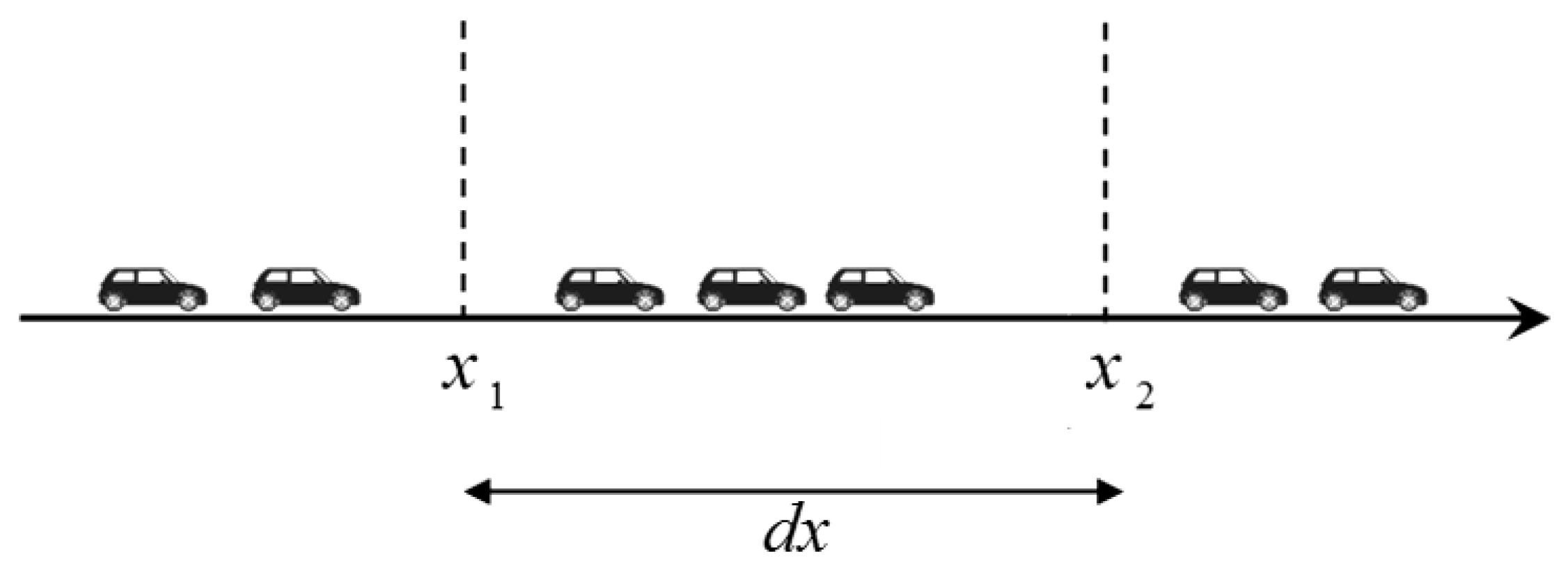
In this work, we assume that the flow Q is a function with a fractional index α and can be expanded as a series following the Theorem 1. To set up the mathematical statement of the fractional transport density equation, the traffic flow into and out of the R S = [ x 1 , x 2 ] in the highway is considered in Eulerian description. We are interested in the density of vehicles which flow in at point x 1 and out at point x 2 as shown in Figure 2.
Starting from the classical calculus for unsteady flow we define the density as [27],
ρ ( x , t ) = N O V f r o m x 1 t o x 2 d x
and the flow as,
Q ( x , t ) = N O V f r o m t 1 t o t 2 d t
During this study vehicles are neither created (entrance) nor destroyed (exit). Therefore, we follow the same methodology used in the fluid mechanic in derivation of the continuity equation. So based on the hydrodynamic relationship we have,
Q ( x 1 ) = ρ v
where ρ and v are the density and velocity, respectively. Q ( x 1 ) represents the flow into the R S . Though, the flow out of the R S is estimated according to Taylor expansion around x 1 as,
Q ( x 2 ) = ρ v + ( ρ v ) x d x + 1 2 ! 2 ( ρ v ) x 2 ( d x ) 2 +
So,
Q ( x 2 ) Q ( x 1 ) = ( ρ v ) x d x + 1 2 ! 2 ( ρ v ) x 2 ( d x ) 2 +
In classical calculus, particularly in fluid dynamic, it is widely confirmed that we truncate this series so we ignore terms higher than order d x , so Equation (15) becomes,
Q ( x 1 ) Q ( x 2 ) = ( ρ v ) x d x
However, this truncation indicates that the change in flux is linear which is not only considered as a limitation for the traffic flow theory, but also for various areas of science and engineering.
On the other side, in fractional calculus, it was proven that the mass ( N O V ) obeys the power law with respect to length scale of the spatial coordinate as [28,29],
N O V ( x , α ) x α
where α ( 0 ,   1 ] is the fractal parameter describing the order of space-derivative; therefore, we assume that the traffic flow is following the real-order power-laws as,
Q ( x ) = x λ
where λ . Substituting Equation (17) into Equation (4) yields,
D 0 α x λ = Γ ( 1 + λ ) Γ ( 1 + λ α ) x λ α
Now, based on Equation (17) we define,
Q ( x 2 ) Q ( x 1 ) = x 2 λ x 1 λ
or,
Q ( x 2 ) = Q ( x 1 ) + ( x 2 λ x 1 λ )
Expanding Q ( x 2 ) about x 1 using fractional Taylor power series defined in Theorem 1, one can obtain,
Q ( x 2 ) = Q ( x 1 ) + D 0 α ( x 1 λ ) Γ ( 1 + α ) ( x 2 α x 1 α ) + D 0 α D 0 α ( x 1 λ ) Γ ( 1 + 2 α ) x 1 α ( x 2 α x 1 α ) +
As long as the flow in Equation (21) is represented as polynomial with non-negative real power, the fractional Taylor expansion is exact if the fractional α o r d e r equals the λ degree polynomial as we explained in Section 3.
Thus, setting α = λ and substituting in Equation (18) results,
D 0 α x λ = Γ ( 1 + α ) .
Equation (22) indicates that the Caputo derivative of the proposed flux is constant. So by using zero derivative property introduced in Equation (5) and combining Equation (21) and Equation (22) we obtain,
Q ( x 2 ) = Q ( x 1 ) + ( x 2 α x 1 α ) + 0 +
As a result, setting the fractional α o r d e r equals the λ degree is exactly similar to the concept of truncating the Taylor polynomial after the second term with zero error in order to obtain the exact estimate. Furthermore, setting α = λ we implicitly admit that the flux is nonlinear since D 0 α x λ = Γ ( 1 + α ) is a constant. Because unlike classical derivative, when fractional derivative is constant then the origin function is nonlinear. Let us rewrite Equation (21) as,
Q ( x 2 ) Q ( x 1 ) = D 0 α Q ( x 1 ) Γ ( 1 + α ) ( x 2 α x 1 α ) .
On the other side, in traffic flow theory, since the R S = [ x 1 , x 2 ] is fixed in space, one can conclude easily,
N O V = ρ x 1 x 2 d x = ρ ( x 2 x 1 ) veh .
Further, based on the control volume analysis in fluid dynamics, the time rate of change in N O V in the fixed R S in a differential form is defined as,
d N O V d t = d ρ d t x 1 x 2 d x .
The above equation represents the accumulation. In fact, the length-space in Equation (26) was measured by usual metric d x as the Euclidean distance. Nevertheless, this argument is valid for the standard measure in metric space d x , but not for the fractional space. Hence, we need to adopt a fractional measure, namely d M α ( x ) . Now, based on the fractal geometry, this relation between the fractional and classical measures takes the form as concluded in [30,31],
d M α ( x ) = ψ ( α , x ) d x .
Clearly, the fractional transformation ψ ( α , x ) between the two spaces, must be written in power law to reflect fractality [32,33], which means spatial scale dependence of space. Notably, the transformation ψ ( α , x ) can take many forms based on what type of fractional integral we adopt. Here, in this study, we consider the Riemann–Liouville fractional integral. It is stated in [34,35] that the fractional variable measure is defined as,
d M α ( x ) = x α 1 Γ ( α ) d x
Now, we define the fractional measure for the region R S of 1-dimentional space as [36],
M α ( S R ) = R S d M α ( x ) = 1 Γ ( α ) R S x α 1 d x < + for   any   R S +
Notice that when α = 1 , we recover to the Euclidean distance in + as,
M 1 ( S R = [ x 1 , x 2 ] ) = 1 Γ ( 1 ) R S x 1 1 d x = ( x 2 x 1 )
For a fractional generalization for the Equation (26), we apply the fractional variable measure d M α ( x ) as,
N O V t = ρ t x 1 x 2 d M α ( x ) = ρ t 1 Γ ( α ) x α α | x 1 x 2 = ρ t x 2 α x 1 α Γ ( 1 + α ) .
Intuitively, analogous to derivation of the balance law in continuum mechanics that mass ( N O V ) is conserved, accordingly for the fixed R S the sum of the accumulation inside the R S and fluid that is flowing out of the R S must be equal to the amount of fluid flowing into the R S . That is,
N O V t + Q ( x 2 ) = Q ( x 1 ) ,
so,
Δ Q ( x ) = N O V t .
Combining Equations (24), (30), and (32) yields,
D 0 α Q ( x 1 ) Γ ( 1 + α ) ( x 2 α x 1 α ) = ρ t x 2 α x 1 α Γ ( 1 + α ) ,
by simple calculation and using the differential symbol,
ρ ( x , t ) t + α Q ( x , t ) x α = 0 .
This is a differential statement of conserved N O V which is referred to as the space-fractional transport density equation or simply the space-fractional LWR model (F-LWR).
Regarding the units, the conventional space operator x has dimensions of inverse kilometers km 1 , while the fractional space derivative operator α x α has, km α . Thus, in order to be consistent with the space dimensionality we introduce the new parameter σ in the following way,
1 σ 1 α α x α = 1 km for   α ( 0 ,   1 ] .
In this manner, the model is dimensionally consistent if the new parameter σ has dimension of space as, [ σ ] = km . Then, replacing x in classical LWR by 1 σ 1 α α x α , we obtain a consistent model. However, for simplicity we take σ = 1 in this work, accordingly Equation (34) is dimensionally consistent.
Later, in similar fashion, one can extend this model to space and time-fractional LWR model as [17,18,19],
β ρ ( x , t ) t β + α Q ( x , t ) x α = 0

5. Characteristics Method

Many attempts have been made to address the fractional transport equation using different fractional operators aligned with different methods. Wang et al. [17] studied the F-LWR model using local fractional conservation laws based on the fractional vector integrals. Meanwhile, Li et al. [37] used the fractional Laplace variational iteration method in Hausdorff fractional derivative sense. Wu [38] used modified Riemann–Liouville operator and the fractional Jumarie–Taylor’s series of multivariate functions. Dubey et al. [39] approached the F-LWR using the homotopy analysis method along with the Mittag-Leffler function in fractal space.
However, in this study, we implemented the characteristics method aligned with the GFD fractional derivative, then traffic simulation to detect the effects of the fractional order was provided.
In fact, it is proven that smooth or classical solutions of the continuity equation does not exist. Yet, this model arises in physics so some solutions exist. Thus, any suggested solutions can only be formed within a space of nondifferentiable functions at some points ( x N o n d i f f , t N o n d i f f ) , namely the weak solutions [40,41,42].
Consider the Cauchy problem of the fractional LWR model as,
t ρ ( x , t ) + α x α Q ( x , t ) = 0 ,   0 < α 1
ρ ( x , 0 ) = ρ 0 ( x ) .
Before constructing a weak solution, however, we provide some preliminary relations. Under uninterrupted flow conditions, speed, density, and flow are all related by the fundamental relation,
Q = v ρ
Moreover, the speed and density are linked by the Greenshields relation [43],
v = v m ( 1 ρ ρ m )
where v m , ρ m are the maximum speed and density allowed on a road, respectively. So, one can find,
Q = ( v m ρ v m ρ m ρ 2 ) ,
substituting Equation (37) into Equation (36) to obtain,
t ρ ( x , t ) + α x α ( v m ρ v m ρ m ρ 2 ) = 0 ,
using properties (6)–(10) yields,
t ρ ( x , t ) + ( v m 2 v m ρ m ρ ) Γ ( β ) Γ ( β + 1 α ) x 1 α x ρ ( x , t ) = 0 ,
therefore, the characteristic equations are provided by,
x α 1 d x d s = Γ ( β ) Γ ( β + 1 α ) ( v m 2 v m ρ m ρ ) d t d s = 1 d ρ d s = 0 .
.
Subject to the initial conditions,
{ t ( r , 0 ) = 0 x ( r , 0 ) = ( α r ) 1 / α ρ ( r , 0 ) = ψ ( r ) ,
integrating system (40), we obtain,
{ x = α Γ ( β ) Γ ( β + 1 α ) ( v m 2 v m ρ m ρ ) s + α c 1 ( r ) α t = s + c 2 ( r ) ρ = ψ ( r ) .
To determine the r-dependence, c 1 ( r ) and c 2 ( r ) we use the initial conditions (41),
{ x = α ( v m 2 v m ρ m ρ ) Γ ( β ) Γ ( β + 1 α ) t + r α t = s ρ = ψ ( r ) .
So,
r = x α α Γ ( β ) Γ ( β + 1 α ) ( v m 2 v m ρ m ρ ) t .
Therefore, the solution of the initial value problem can be written as,
ρ ( x , t ) = ψ ( x α α Γ ( β ) Γ ( β + 1 α ) ( v m 2 v m ρ m ρ ) t ) ,
where ψ ( x , t ) is an arbitrary function. For simplicity, we take ψ ( θ ) = θ and substitute in Equation (45) to obtain,
ρ = ρ m ( Γ ( β + 1 α ) x α α Γ ( β ) v m t ) ρ m Γ ( β + 1 α ) 2 α Γ ( β ) v m t .
According to Malaysian Institute of Road Safety Research (MIRO) the speed limit is v m = 80 km/h and suppose that the average length of a car is about 5 m, thus the maximum density is ρ m = 200 veh/km. For the sake of simplicity, we also set β = 1 . Therefore,
ρ = 5 ( Γ ( 2 α ) x α 80 α t ) 5 Γ ( 2 α ) 4 α t .
Taking the Riemann problem as piecewise constant initial data which represent a red signal light as,
ρ ( x , t ) = { ρ l = 110 ; x < s t + ε 0 ρ r = 200 ; x > s t + ε 0 ,
where ε 0 + and ρ l , ρ r represent the values of the density on the R S at the left and at the right, respectively. Moreover, s is the propagation speed which can be found from the jump condition,
s = 1 ρ r ρ l ρ l ρ r Γ ( β ) Γ ( β + 1 α ) ( v m 2 v m ρ m ρ ) x 1 α d ρ = 44 Γ ( β ) Γ ( β + 1 α ) x 1 α .
So, system (48) can be expressed as,
ρ ( x , t ) = { ρ l = 110 ; x < 44 Γ ( β ) Γ ( β + 1 α ) x 1 α t + ε 0 ρ r = 200 ; x > 44 Γ ( β ) Γ ( β + 1 α ) x 1 α t + ε 0 .
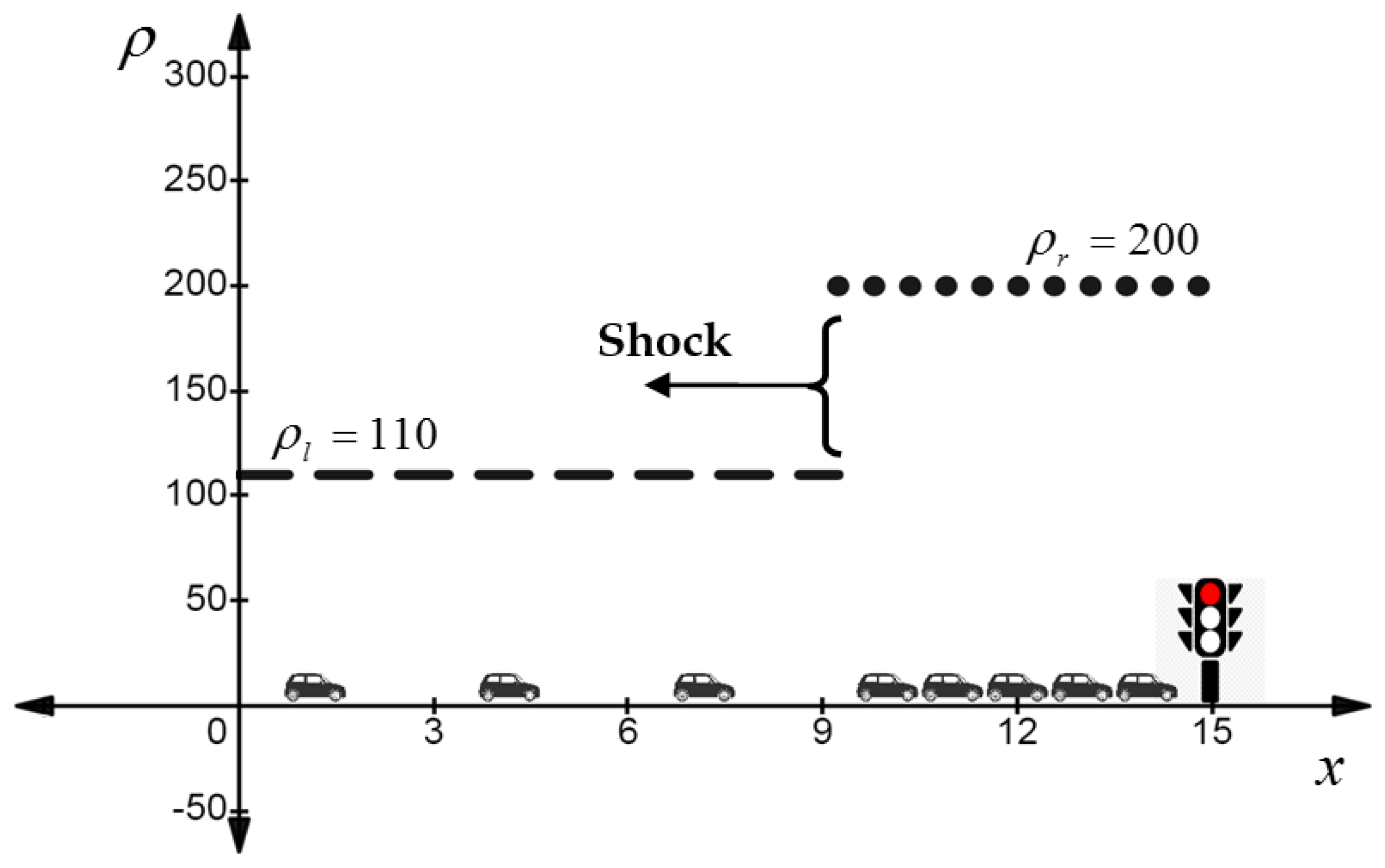
Clearly, system (50) is a discontinuous solution for Equation (39). In fact, it represents a red-light traffic where the density increases dramatically from ρ l = 110 to ρ r = 200 and forms a shock wave at x = ε 0 in finite time. This jam wave propagates against the stream to form a queue in front of the traffic signal, and it moves with negative speed, s satisfying the Rankine–Hugoniot jump condition,
s = 44 Γ ( β ) Γ ( β + 1 α ) x 1 α
as shown in Figure 3. Unlike the classical calculus, the jam speed now depends on the fractional order α . Moreover, the most important part is that each traffic signal has its own character based on the value of the fractional order α . Therefore, using the fractional model, the traffic engineers can predict various locations and speeds of the shock wave for each traffic signal.
It turns out that, according to Table 1, by increasing the value of α the shock wave speed decreases, as a result the shock location increases.
However, in general, when the traffic signal light turns red the drivers reduce their speeds gradually, not sharply. Thus, we are interested in constructing a continuous solution corresponds to Riemann problem. Hence, we look for a solution which continuously connects the density from left ρ l with the density from right ρ r , namely, the weak solution.
To perform this we set,
110 < 5 ( Γ ( 2 α ) x α 80 α t ) 5 Γ ( 2 α ) 4 α t < 200 .
Therefore, the solution takes the form as,
ρ ( x , t ) = { ρ l = 110 ; x < 110 Γ ( 2 α ) 8 α t Γ ( 2 α ) α ρ s y n c = 5 ( Γ ( 2 α ) x α 80 α t ) 5 Γ ( 2 α ) 4 α t ; 110 Γ ( 2 α ) 8 α t Γ ( 2 α ) α x ρ r = 200 ; x < 200 Γ ( 2 α ) 80 α t Γ ( 2 α ) α , 200 Γ ( 2 α ) 80 α t Γ ( 2 α ) α
where ρ s y n c is the synchronized density phase, so the drivers inside this phase adjust their speeds according to the jam ahead.
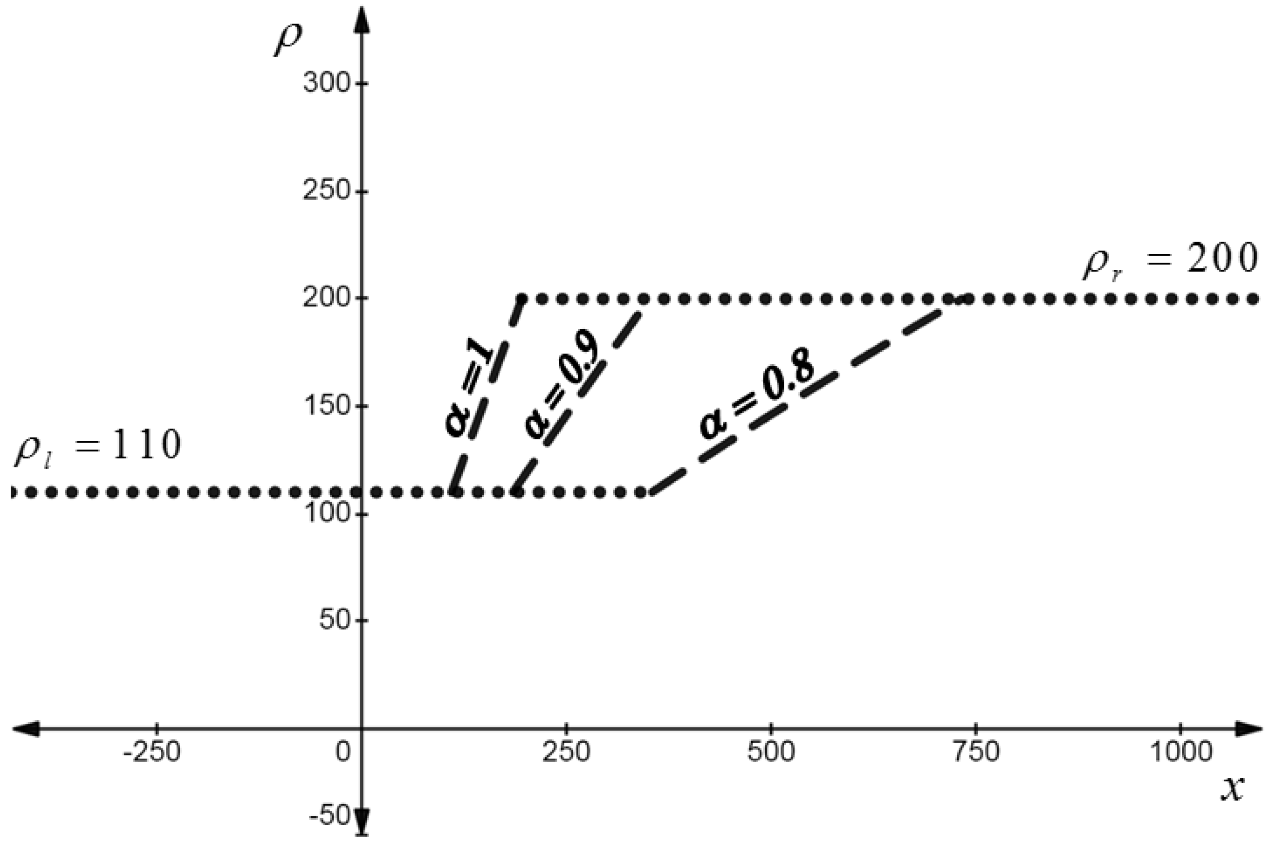
Now, to illustrate the effects of the non-integer fractional order on the proposed model we vary the value of fractional order in Equation (52) with α = 0.8 ,   0.9 and 1, in which the last value belongs to classical calculus. We denote the drivers who follow α = 0.8 character by 0.8 drivers. Mathematically speaking, as the value of the fractional order increases, the density profile tends to be more linear, as shown in Figure 4. Yet, the significance of the current work lies in the physical interpretation of varying the fractional order. Evidently, the space interval of the synchronized density phase for the 0.8 drivers is longer than 0.9 drivers, which indicates that the latter drivers decrease their speeds sharper than 0.8 drivers. Put differently, the larger the α value , the more aggressive driving style due to the fact that the 0.8 drivers have sufficiently enough space to reduce their speeds gradually in reference to the jam ahead. Meanwhile, in the classical calculus mode when α = 1 the synchronized density recovers to a linear function in space.
The fractional-order value can be empirically set using traffic detector data for a long period of time for each signal. However, we recommend data collected based on the Global Positioning System (GPS) where the mean difference between two densities is not significant at less than 5% error.
So far, however, all previous studies have introduced only numerical solutions with no traffic simulation while the current study provides exact analytical solutions and vehicular simulation associated to successive signalized intersections. As some research has been carried out on a fractional LWR model, only two studies have attempted to deal with linear speed–density relationship. Singh et al. [44] solved various F-LWR models numerically using a constant, linear, and non-linear speed–density relation and obtained nondifferentiable solutions, while this works uses exact solutions through Equation (52) which are considered differentiable almost everywhere. Wang et al. [17], derived the F-LWR model based on the fractional vector integrals and used a linear velocity to introduce the Cauchy problem of the nonlinear F-LWR model; however, the authors did not solve the model. On the other side, concerning the constant velocity, Li et al. [37] applied the fractional Laplace transform to solve the model, nevertheless the authors assumed that the vehicles’ speed is 1 km/h and gained nondifferentiable solutions. Similarly, both Jassim [19] and Kumar et al. [18] used the hyperbolic boundary condition along with constant velocity to obtain nondifferential solutions. Finally, in contrast to the abovementioned works, the results of this study are exact and analytic; therefore, there are less computations with guaranteed accuracy.

6. Discussion

In designing smart transportation infrastructure, traffic engineers are highly recommended to determine the proper value of the fractional order that can fit each specific traffic signal on the road which can be found by using various hardware, such as cameras and sensors or software such as GPS applications. Knowing the α value is of great importance so that the traffic engineers can predict various speeds of the jam for a particular traffic signal on road so as to construct the best locations of some successive signals. As a further advantage of using the fractional model, the traffic engineers can set the best waiting time at a red-light traffic in order to prevent the jam wave from reaching the next signal.
Example. 
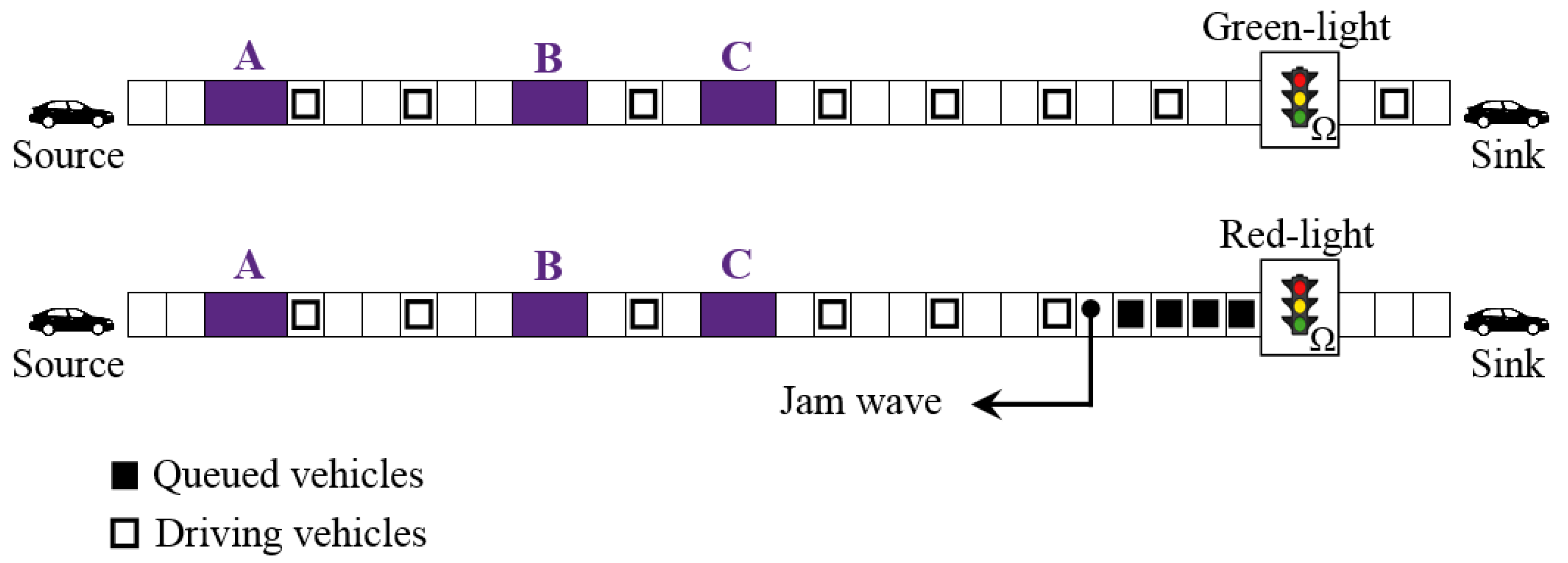
In this simulation we adopt the Riemann problem Equation (50), so a comparison between two different scenarios when α 1 = 0.90 and α 2 = 0.95 is conducted with the purpose of describing the implications and benefits of the fractional model in constructing successive signalized junctions. Now, let us assume a traffic signal is sited at the location x = 15 km, mentioned as Ω-signal, where a traffic engineer plans to set another traffic signal on the left and has only three choices, location A = 14 , B = 14.2 or C = 14.3 as shown in Figure 5. Taking into account that the jam wave results from the red-light of the Ω-signal is not allowed to reach the proposed locations A, B or C, given that the Ω-signal shows a red light for 50 s, a green light for 50 s, and a yellow light for 2 s. Thus, it is of fundamental importance that the Ω-signal turns green before the jam wave reaches the proposed locations.
As the Ω-signal light turns red, traffic starts backing up to the left, and the speed of the backward propagation of a queue is provided as Equation (49). Hence, the jam wave location is,
x | Shock location = 44 Γ ( β ) Γ ( β + 1 α ) x 1 α t + 15 .
Substituting x = 14 ,   14.2 and 14.3 km in Equation (53) yields the expected durations of jam wave to reach the given locations as shown in Table 2.
Based on Table 2, the traffic engineer has two different scenarios. First, if the Ω-signal behaves under the α 1 order effect, then locations B and C are definitely rejected as the traffic jam arrives to them before the Ω-signal turns green, meanwhile, as the queue reaches location A, the Ω-signal already turned green about 7 s ago considering 2 s for the yellow light. Hence, location A is the only reasonable option. Second, if α 2 controls the Ω-signal behavior, then location C is out of the scope because its expected duration is less than 50 s. In fact, locations A and B are clearly accepted. So, the proper decision depends on the value of the fractional order which is considered the crucial component of the jam wave speed and location.

7. Conclusions

In this study, we established and solved a new fractional generalization for the continuity equation, particularly the F-LWR model. As a pursuit of these we herein match the degree and the order for the Caputo fractional Taylor expansion, consequently we obtain zero error and the exact value. Then, we link the fractional measure with Riemann–Liouville fractional integral on space scale to obtain a relation between the single variable measure of fractional space and the measure of integer space. Advantageously, this extension from classical to fractional space eliminated the linear restriction of the flux in the road segment; therefore, various nonlinear and complex behaviors of the traffic flow can be predicted, such as nonhomogeneous driving style. Verifying nonlinearity for the fractional transport equation is of paramount importance not only for the traffic flow theory, but also for several fields of physics such as hydrodynamics, electromagnetism, and quantum mechanics. In the last part, two different solutions are obtained by using the characteristics method in line with the generalized fractional derivative. Consequently, the effects of the fractional-order derivative are simulated in regard to traffic signals. As a future scope of the work, we suggest extending this model to a space and time fractional LWR model in order to analyze the impact of the time dependent variable order.

Author Contributions

Original draft preparation, investigation, conceptualization, analysis R.M.S.; review, editing and supervision S.S.J. All authors have read and agreed to the published version of the manuscript.

Funding

This research received no external funding.

Institutional Review Board Statement

Not applicable.

Informed Consent Statement

Not applicable.

Data Availability Statement

Not applicable.

Conflicts of Interest

The authors declare no conflict of interest.

References

  1. Erramilli, A.; Willinger, W.; Pruthi, P. Fractal traffic flows in high-speed communications networks. Fractals 1994, 2, 409–412. [Google Scholar] [CrossRef]
  2. Chen, W.; Sun, H.; Zhang, X.; Korošak, D. Anomalous diffusion modeling by fractal and fractional derivatives. Comput. Math. Appl. 2010, 59, 1754–1758. [Google Scholar] [CrossRef] [Green Version]
  3. Magin, R.L. Fractional Calculus in Bioengineering; Begell House: Danbury, CT, USA, 2006. [Google Scholar]
  4. Hadid, S.B.; Ibrahim, R.W.; Altulea, D.; Momani, S. Solvability and stability of a fractional dynamical system of the growth of COVID19 with approximate solution by fractional Chebyshev polynomials. Adv. Differ. Equ. 2020, 2020, 338. [Google Scholar] [CrossRef]
  5. Iqbal, N.; Akgul, A.; Shah, R.; Bariq, A.; Mossa Al-Sawalha, M.; Ali, A. On solutions of fractional-order gas dynamics equation by effective techniques. J. Funct. Spaces 2022, 2022, 3341754. [Google Scholar] [CrossRef]
  6. Mainardi, F. Fractional Calculus: Some Basic Problems in Continuum and Statistical Mechanics. In Fractals and Fractional Calculus in Continuum Mechanics; Springer: New York, NY, USA, 1997. [Google Scholar]
  7. Laskin, N. Fractional market dynamics. Phys. A Stat. Mech. Its Appl. 2000, 287, 482–492. [Google Scholar] [CrossRef]
  8. Bagley, R.L.; Calico, R.A. Fractional order state equations for the control of viscoelastically damped structures. J. Guid. Control Dyn. 1991, 14, 304–311. [Google Scholar] [CrossRef]
  9. Ali, F.; Sheikh, N.A. Introductory Chapter: Fluid Flow Problems. In Fluid Flow Problems; IntechOpen: London, UK, 2018. [Google Scholar]
  10. Lighthill, M.J.; Whitham, G.B. On kinematic waves-II. A theory of traffic flow on long crowded roads. Proc. R. Soc. London Ser. A Math. Phys. Sci. 1955, 229, 317–345. [Google Scholar]
  11. Richards, P.I. Shock waves on the highway. Oper. Res. 1956, 4, 42–51. [Google Scholar] [CrossRef]
  12. Mason, A. Advanced Differential Equations; ED-Tech: London, UK, 2019. [Google Scholar]
  13. Peitgen, H.-O.; Jurgens, H.; Saupe, D. Chaos and Fractals. In New Frontiers of Science; Springer: Berlin/Heidelberg, Germany, 1992. [Google Scholar]
  14. Boris, S.K. Complex dynamics of traffic management. In Encyclopedia of Complexity and Systems Science; Springer: New York, NY, USA, 2009. [Google Scholar]
  15. May, A.D. Traffic Flow Fundamentals; Prentice Hall: Englewood Cliffs, NJ, USA, 1990. [Google Scholar]
  16. Shang, P.; Wan, M.; Kama, S. Fractal nature of highway traffic data. Comput. Math. Appl. 2007, 54, 107–116. [Google Scholar] [CrossRef] [Green Version]
  17. Wang, L.F.; Yang, X.J.; Baleanu, D.; Cattani, C.; Zhao, Y. Fractal dynamical model of vehicular traffic flow within the local fractional conservation laws. Abstr. Appl. Anal. 2014, 2014, 1–5. [Google Scholar] [CrossRef] [Green Version]
  18. Kumar, D.; Tchier, F.; Singh, J.; Baleanu, D. An efficient computational technique for fractal vehicular traffic flow. Entropy 2018, 20, 259. [Google Scholar] [CrossRef]
  19. Jassim, H.K. On approximate methods for fractal vehicular traffic flow. TWMS J. App. Eng. Math. 2017, 7, 58–65. [Google Scholar]
  20. Wheatcraft, S.W.; Meerschaert, M.M. Fractional conservation of mass. Adv. Water Resour. 2008, 31, 1377–1381. [Google Scholar] [CrossRef]
  21. Almeida, R. A Caputo fractional derivative of a function with respect to another function. Commun. Nonlinear Sci. Numer. Simul. 2017, 44, 460–481. [Google Scholar] [CrossRef] [Green Version]
  22. Podlubny, I. Fractional Differential Equations; Academic Press: San Diego, CA, USA, 1999; ISBN 0-1255-8840-2. [Google Scholar]
  23. Abu-Shady, M.; Kaabar, K.A. A Generalized definition of the fractional derivative with applications. Math. Probl. Eng. 2021, 2021, 1–9. [Google Scholar] [CrossRef]
  24. Martínez, F.; Kaabar, K.A. A Novel theoretical investigation of the Abu-Shady–Kaabar fractional derivative as a modeling tool for science and engineering. Comput. Math. Methods Med. 2022, 2022, 1–8. [Google Scholar] [CrossRef] [PubMed]
  25. Usero, D. Fractional Taylor Series for Caputo Fractional Derivatives: Construction of Numerical Schemes. 2008. Preprint. Available online: http://www.fdi.ucm.es/profesor/lvazquez/calcfrac/docs/paper_Usero.pdf (accessed on 2 June 2022).
  26. Vargas, A.M. Finite difference method for solving fractional differential equations at irregular meshes. Math. Comput. Simul. 2022, 193, 204–216. [Google Scholar] [CrossRef]
  27. Olayode, I.O.; Tartibu, L.K.; Campisi, T. Stability analysis and prediction of traffic flow of trucks at road intersections based on heterogenous optimal velocity and artificial neural network model. Smart Cities 2022, 5, 1092–1114. [Google Scholar] [CrossRef]
  28. Ostoja-Starzewski, M.; Li, J.; Joumaa, H.; Demmie, P. From fractal media to continuum mechanics. ZAMM 2014, 94, 373–401. [Google Scholar] [CrossRef]
  29. Cai, W.; Chen, W.; Wang, F. Three-dimensional Hausdorff derivative diffusion model for isotropic/anisotropic fractal porous media. Therm. Sci. 2018, 22, S1–S6. [Google Scholar] [CrossRef]
  30. Tarasov, V. Anisotropic fractal media by vector calculus in non-integer dimensional space. J. Math. Phys. 2014, 55, 083510. [Google Scholar] [CrossRef] [Green Version]
  31. El-Nabulsi, R.A.; Anukool, W. Quantum dots and cuboid quantum wells in fractal dimensions with position-dependent masses. Appl. Phys. A 2021, 127, 856. [Google Scholar] [CrossRef]
  32. Balankin, A.S. A continuum framework for mechanics of fractal materials I: From fractional space to continuum with fractal metric. Eur. J. Phys. B 2015, 88, 90. [Google Scholar] [CrossRef]
  33. El-Nabulsi, R.A.; Anukool, W. Fractal dimension modeling of seismology and earthquakes dynamics. Acta Mech. 2022, 233, 2107–2122. [Google Scholar] [CrossRef]
  34. Tarasov, V.E. Fractional Dynamics: Applications of Fractional Calculus to Dynamics of Particles, Fields, and Media; Springer: Berlin, Germany, 2010. [Google Scholar]
  35. Li, J.; Ostoja-Starzewski, M. Comment on hydrodynamics of fractal continuum flow and map of fluid flow in fractal porous medium into fractal continuum flow. Phys. Rev. E 2013, 88, 057001. [Google Scholar] [CrossRef] [PubMed] [Green Version]
  36. Tarasov, V.E. Fractional systems and fractional Bogoliubov hierarchy equations. Phys. Rev. E 2005, 71, 0111102. [Google Scholar] [CrossRef] [PubMed] [Green Version]
  37. Li, Y.; Wang, L.F.; Zeng, S.D.; Zhao, Y. Local fractional Laplace variational iteration method for fractal vehicular traffic flow. Adv. Theor. Math. Phys. 2014, 2014, 649318. [Google Scholar] [CrossRef]
  38. Wu, G.C. A fractional characteristic method for solving fractional partial differential equations. Appl. Math. Lett. 2011, 24, 1046–1050. [Google Scholar] [CrossRef] [Green Version]
  39. Dubey, V.P.; Kumar, D.; Alshehri, H.M.; Dubey, S.; Singh, J. Computational analysis of local fractional LWR model occurring in a fractal vehicular traffic flow. Fractal Fract. 2022, 6, 426. [Google Scholar] [CrossRef]
  40. Dafermos, C. Hyperbolic Conservation Laws in Continuum Physics; Springer: Berlin, Germany, 2000. [Google Scholar]
  41. Glimm, J.G. Solutions in the large for nonlinear hyperbolic systems of equations. Commun. Pure Appl. Math. 1965, 18, 697–715. [Google Scholar] [CrossRef]
  42. Daganzo, C.F.; Geroliminis, N. An analytical approximation for the macroscopic fundamental diagram of urban traffic. Transp. Res. Part B Methodol. 2008, 42, 771–781. [Google Scholar] [CrossRef]
  43. Greenshields, B.D. A study of traffic capacity. In Proceedings of the Fourteenth Annual Meeting of the Highway Research Board, Washington, DC, USA, 6–7 December 1934; pp. 448–477. Available online: http://pubsindex.trb.org/view.aspx?id=120649 (accessed on 8 March 2022).
  44. Singh, N.; Kumar, K.; Goswami, P.; Jafari, H. Analytical method to solve the local fractional vehicular traffic flow model. Math. Methods Appl. Sci. 2022, 45, 3983–4001. [Google Scholar] [CrossRef]
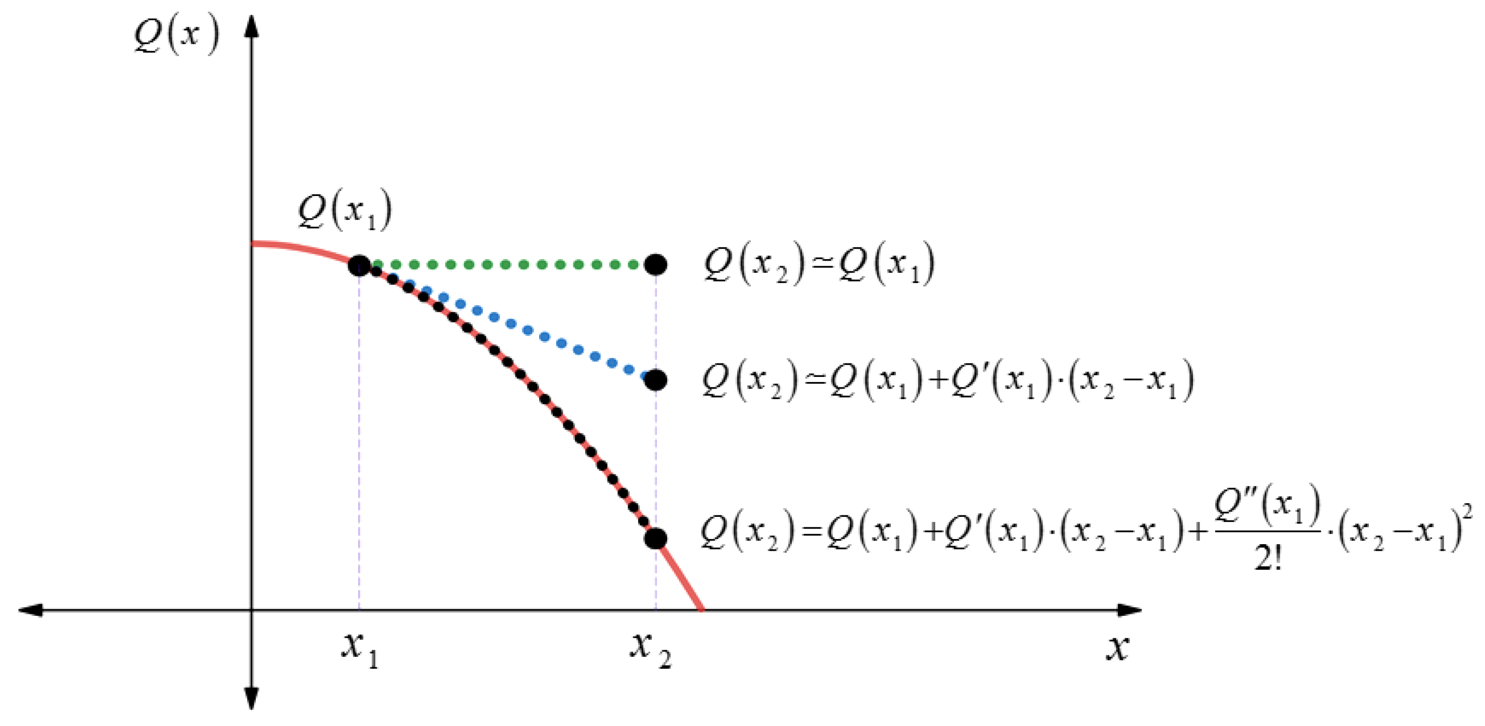
Figure 1. Second-order Taylor approximation around x 1 to obtain the exact value for a quadratic function at x 2 .
Smartcities 05 00084 g001
Figure 2. Schematic diagram for fixed road segment R S in a moving traffic.
Smartcities 05 00084 g002
Figure 3. Schematic diagram for moving shock wave start at the location x = 15 km with α = 0.7 and t = 0.06 h .
Smartcities 05 00084 g003
Figure 4. Density in the space. Exact solution at time t = 0.2 hours for different fractional-order values, α = 0.8 , α = 0.9 , and α = 1 .
Smartcities 05 00084 g004
Figure 5. Schematic diagram describes the formation of travelling jam moves towards three different locations A, B, and C.
Smartcities 05 00084 g005
Table 1. Shock location and speed for various fractional-order values.
Time (h)Fractional OrderShock Location (km)Shock Speed (km/h)
t = 0.06 α = 0.1 x = 4.459 s = 175.67
α = 0.3 x = 5.462 s = 158.93
α = 0.7 x = 9.263 s = 95.600
Table 2. Durations in seconds of the shock wave to reach various locations A, B, and C using different values of the fractional order.
ABC
α 1 = 0.90 59.7847.7541.75
α 2 = 0.95 69.8055.8048.81
Publisher’s Note: MDPI stays neutral with regard to jurisdictional claims in published maps and institutional affiliations.