Novel Method for Speeding Up Time Series Processing in Smart City Applications

Abstract

The huge amount of daily generated data in smart cities has called for more effective data storage, processing, and analysis technologies. A significant part of this data are streaming data (i.e., time series data). Time series similarity or dissimilarity measuring represents an essential and critical task for several data mining and machine learning algorithms. Consequently, a similarity or distance measure that can extract the similarities and differences among the time series in a precise way can highly increase the efficiency of mining and learning processes. This paper proposes a novel elastic distance measure to measure how much a time series is dissimilar from another. The proposed measure is based on the Adaptive Simulated Annealing Representation (ASAR) approach and is called the Adaptive Simulated Annealing Representation Based Distance Measure (ASAR-Distance). ASAR-Distance adapts the ASAR approach to include more information about the time series shape by including additional information about the slopes of the local trends. This slope information, together with the magnitude information, is used to calculate the distance by a new definition that combines the Manhattan, Cosine, and Dynamic Time Warping distance measures. The experimental results have shown that the ASAR-Distance is able to overcome the limitations of handling the local time-shifting, reading the local trends information precisely, and the inherited high computational complexity of the traditional elastic distance measures.

1. Introduction

In recent years, smart cities have witnessed the creation of huge volumes of data with businesses growing more automated and communication technologies progressing. For instance, the global Internet of Things (IoT) industry has become vast and rapidly expanding. It is estimated that IoT connected devices would reach over 41 billion, generating 79.4 zettabytes of data by 2025 [1]. A serious proportion of this continuously generated data is streaming data or time series data (i.e., a succession of real values in time order). The processing and analysis of such a vast amount of data represent a real challenge for operating data-based smart city services [2]. As this massive amount of data contains very useful information for optimizing smart city services and achieving sustainable development goals (including sustainable cities), it became crucial to develop more effective time-series data storage, processing, and analysis methods [3,4,5]. The data comes from various smart city sectors and usually carries useful knowledge about the source sector. For instance, time series data comes from and is also utilized in smart agriculture [6], smart energy [7], smart health [8], smart transport [9], and several smart city services [10,11,12].

Machine learning algorithms can extract meaningful knowledge from time series data [13,14]. Such algorithms need to study and analyze the historical behavior of time series. Some of the tasks may also need to measure the similarity/distance between time series such as anomaly detection [15], clustering [16], classification [17], and motif discovery [18]. The similarity measure explains how much one time series is similar to another, while the distance measure explains how much they are different. Consequently, the two terms will be used interchangeably in this paper. Measuring the similarity between time series adds high computation complexity to these algorithms, especially for high-dimensional time series. Consequently, traditional similarity measures, which use the time series in its raw form, require more computation resources to achieve an efficient processing time. In our previous research [19], we have proposed the Adaptive Simulated Annealing Representation (ASAR) approach. ASAR has shown its ability to represent the time series data in much lower dimensionality while preserving the shape of the time series, addressing the big data storage challenge in smart cities. Moreover, ASAR can reduce the computation complexity of any machine learning task that needs to measure similarity by lowering the dimensionality of the data.

ASAR has no constraints for using a particular similarity measure after transforming the data to the new representation. Therefore, it has introduced a new solution for reducing the computation complexity overhead by storing the time series data in ASAR form. However, a proper similarity measure is needed to increase the accuracy by making it able to read more information about the time series shape. The similarity measures in the literature suffer from various problems. Some measures are straightforward, such as the Euclidean distance [20], but they cannot handle the time shifting in time series data (i.e., time series that have a similar shape but they have segments with different phases). Consequently, such measures fail to discover the similarity in shape efficiently. On the other hand, elastic measures, such as Dynamic Time Warping (DTW) [21], can handle time shifting, but they go with high computation overhead, making them unsuitable for handling large datasets of time series data for smart city services. Moreover, even with the ability to handle time-shifting, the trend information may be read imprecisely. For instance, DTW computes the distance between two points based only on their magnitude without considering the trend information.

To overcome these limitations, we have proposed a novel measure that supports the merits of the elastic measures in handling time shifting, but taking into account the trend information to detect the shape similarity more precisely. Furthermore, by lowering the data dimensionality, the computation overhead is reduced. The proposed measure is firstly adapting ASAR by adding more information about the segments’ slopes to the new representation, which provides more information about the local trends. Then it combines Manhattan distance [22], cosine distance [23], and DTW in one unified distance measure that can compare the similarity between the instances based on not only the magnitude but also the trend information. This distance measure is tailored to study the dissimilarity in shape by keeping only the relevant information of the local trends in the raw time series and comparing this information between the different time series. Therefore, the main contributions of this novel distance measure are the following: it can take into account the original shape of the time series (by keeping the relevant information about the local trends), can handle the local time-shifting, and is able to measure the distance in a much lower dimensionality (as this method needs less computational resources).

The rest of the paper is organized as follows. The related work is presented in Section 2. The proposed distance measure and the experimental evaluation are introduced in Section 3 and Section 4, respectively. The conclusion of this research is presented in Section 5.

2. Related Work

A variety of similarity/distance measures have been proposed in the literature to show how much a time series is similar/dissimilar to another. A distance measure that can reflect the underlying information and the shape similarity between the time series is crucial for various data mining tasks such as time series classification, anomaly detection, and clustering. Part of the proposed measures can be used only with specific time series representations, while the other can be used regardless of the representation form.

The Minkowski distance ($L_p-norms$) [22] and its variants are the most basic time series distance measures. For two time series $T_1$ and $T_2$, Minkowski distance is defined as $L_p(T_1,T_2)=\sqrt[p]{{\sum }_{i=1}^n{|T_{1_i}-T_{2_i}|}^p}$. The Manhattan distance ($L_1-norm$) and the Euclidean distance ($L_2-norm$) are considered as the most popular variants where $p=1$ and $p=2$, respectively. These distance measures allow only one-to-one comparison between time series. In other words, each i-th point in the first time series must be compared with the i-th point in the second time series. These measures are straightforward, easy to implement, and have linear computational complexity. However, they have some drawbacks, such as the two time series must have the same length to compare them. In addition, they are sensitive to the noise and shifting along the time axes. Another distance method that belongs to this group is the cosine distance [23]. It compares the distance between instances based on their trend. However, it does not take the magnitude into account. The issue of Minkowski distance (i.e., being unable to handle local time shifting) has inspired Berndt and Clifford [21] to propose an elastic distance measure called the Dynamic Time Warping (DTW). Unlike $L_p-norms$ and cosine distance measures, DTW allows one-to-many comparison between time series. DTW uses dynamic programming to find an optimal warping path, i.e., the path that minimizes the total cumulative distance between two time series. DTW is widely used in the literature in different tasks such as time series classification and clustering due to its high accuracy and ability to handle time shifting. It is also a parameter-free measure. However, finding the optimal warping path costs high computational complexity (quadratic), making it inefficient for handling time series with large lengths.

More elastic measures have been proposed. Vlachos et al. [24] have proposed the Longest Common Subsequence (LCSS) measure, which gives more weights for the similar parts of the time series. LCSS allows one-to-many/one-to-none comparison between time series. LCSS matches two points in two time series if the distance between them is less than a threshold. Another similarity measure is the Edit Distance on Real sequence (EDR) [25]. Similar to LCSS, EDR compares the distance between two points to a threshold. However, it quantifies the resulted distance as either 0 or 1. In addition, EDR adds penalties in case of a matching gap, where the penalties are based on the gap length. Edit distance with Real Penalty (ERP), a measure that combines the advantages of DTW and EDR, was proposed [26]. ERP sets a reference point. If a distance between two points was larger than a threshold, the distance is computed between one of the points and the reference point instead of between the two points. Chen et al. [27] have proposed the Spatial Assembling Distance (SpADe). SpADe is a warping distance that can handle shifting and scaling in the y and time axes. SpADe looks for the matching segments (patterns) in the two time series, then finds the two time series that contain the most similar matching patterns to show the most similar time series.

Several methods have been proposed in the literature to measure the similarity between time series by converting the time series to another form first. Symbolic representation, known as the Symbolic Aggregate approXimation (SAX), is one of the most extensively used time series representation methods [28,29]. SAX divides the time series into equal-length segments. The mean value of a segment is used to assign a symbol. SAX then calculates the distance between the symbols using a special lookup function. SAX accelerates time series data mining. However, it loses essential information about the local trends during the representation process as it considers only the mean value of the segment (i.e., it does not take into account the trend of the segment). Another method is the symbolic representation of the Fragment Alignment Distance (FAD) method [30]. The Derivative time series Segment Approximation (DSA) method [31] is used by FAD to calculate the derivative of a time series. The derivative sequence is then converted into a symbolic sequence by defining a threshold and comparing it to the derivative estimation value of each sample. Zhang and Pi [30] have proposed two ways to calculate the distance. The first one is simply using the Dynamic Time Warping (DTW) algorithm to measure the distance between two symbolic representations. The second defines a new distance function that compares the fragments instead of the points, where a fragment is a set of successive points with the same symbol. Three scenarios are defined. In the first one, if the symbols of the two fragments are different, then the distance is equal to 1. In the second one, if they are the same, then the distance depends on the length of each fragment. In the third one, if the two series are not equal in length, then some fragments from one of the two series will be without mapped fragments to compare; in that case, the distance is equal to 1, which means these fragments are not similar to any fragment. Kamalzadeh et al. [32] have proposed the bilateral slope-based distance (BSD). BSD is based on their proposed segmentation method, Adaptive Particle Swarm Optimization Segmentation (APSOS) [33]. APSOS segments the time series by looking for the points that best segment the time series. By setting an optimization goal to minimize the error between the raw time series and the segmented time series, these points are found using an adapted particle swarm optimization algorithm. To measure the distance, they have adapted their segmentation method by including the slopes of the segments. BSD uses the slope information and the Euclidean distance to measure the distance between the time series. This addition of the slope information allows for a comparison based on both the magnitude and the trend information.

The methods in the literature have one or more of the following drawbacks: the group of methods that allows one-to-one comparison [22] suffers from an inability to handle the local time-shifting. Moreover, the time series must have a similar length. On the other hand, the other group of methods (the elastic measures) [21,24,25,26,27], which allows one-to-many comparison, suffers from high computational complexity. Transforming the time series into symbolic representation [28,29,30] also comes with several drawbacks, such as losing the local trend information and the original data distribution. We propose a novel distance measure to address and overcome these drawbacks, which will be introduced in detail in the next section.

3. Adaptive Simulated Annealing Representation (ASAR) Based Distance Measure

The distance measure quality highly depends on the measure’s objective (i.e., to discover a similarity/dissimilarity in time, shape, or magnitude). In this paper, we focus on the objective of finding similar patterns in shape where the exact time is not important. For this purpose, time elastic methods such as DTW are preferred. Our time elastic method is capable of measuring the dissimilarity by adapting ASAR to provide more information about the local trends and by combining the DTW with the Manhattan and Cosine distance measures.

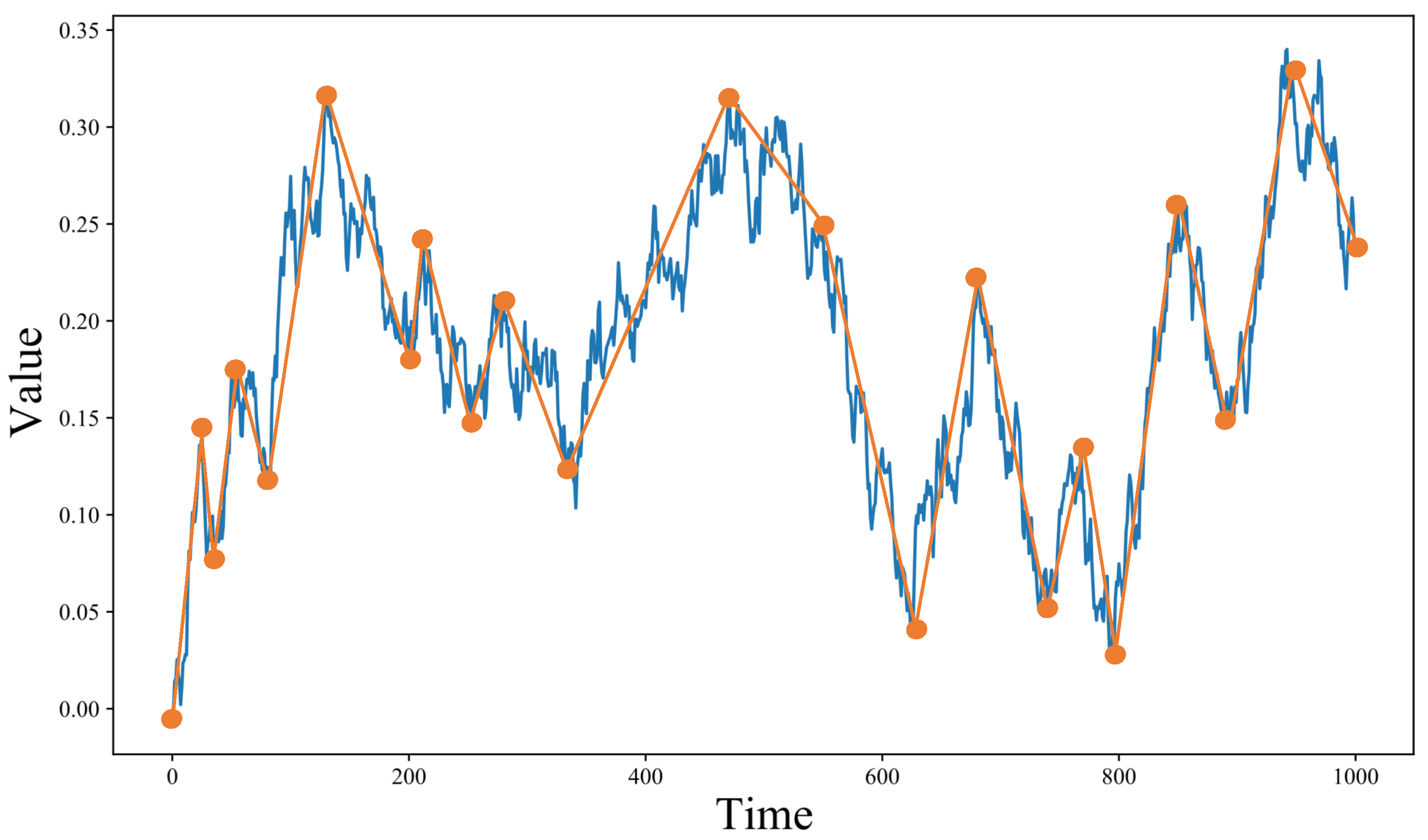
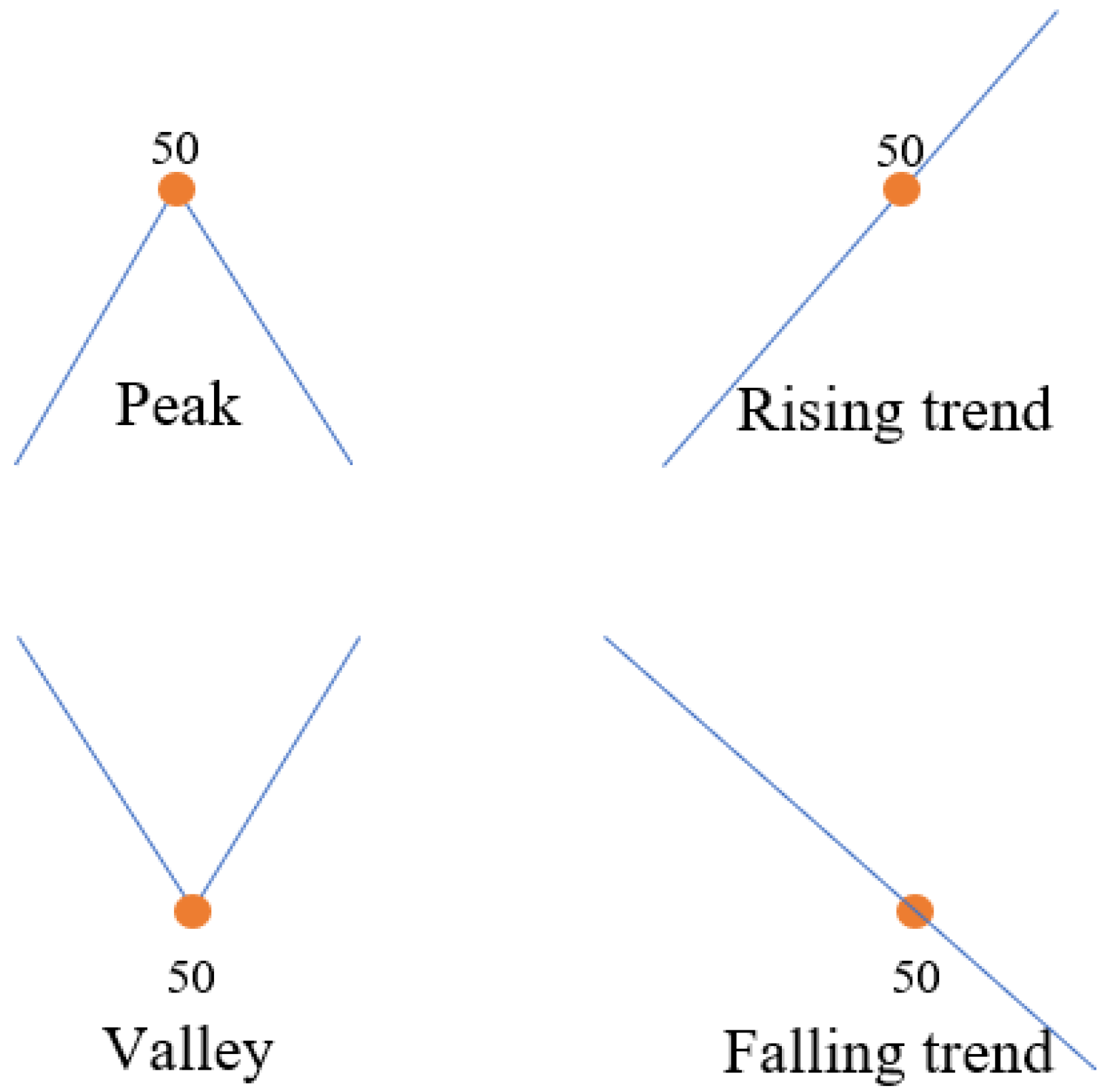
3.1. Adaptive Simulated Annealing Representation (ASAR)

ASAR aims to save storage space when storing time series datasets generated on a daily basis by the sensing infrastructure to be utilized for the optimization of smart city services. At the same time, ASAR aims to fulfill this objective without losing information to make it suitable for future data mining and machine learning tasks. ASAR approaches the representation of time series as an optimization problem. It locates the instances in the raw time series which capture the shape while neglecting the remainder of the instances. Each time series comprises multiple local trends that form a time series shape. Two time series, for example, may have the same shape, implying that they follow the same local trends. The time of occurrence of the local trends, on the other hand, does not have to be the same. Heuristic algorithms can be utilized to solve this optimization problem. To be able to utilize a heuristic algorithm, the time series representation must first be formulated as an optimization problem with the objective of minimizing the time series dimensions while keeping the same shape. Assume X is a time series of length n that is defined as:

$$X=\{X_1,X_2,...,X_n\}$$

The goal of ASAR is to find a new time series R that represents the X time series shape with lower dimensionality. The new representation R can be defined as follows:

$$R=\{R_1,R_2,...,R_k\}$$

(1)

The segments of the new representation R can be used to estimate the corresponding values in the raw time series X. The $R{X}_i$’s approximate corresponding value of $X_i$ can be computed as follows [19]:

$$R{X}_i=\frac{1}{(e-s)}[(i-s)X_e+(e-i)X_s]$$

(2)

s, i, and e are timestamps from the raw time series, where s is the starting point of the segment where i locate, and e is the endpoint of this segment. The proof and more details are shown in the original paper [19].

The approximate values ($R{X}_i\forall s<i<e$) are used to calculate the Mean of Squared Errors ($MSE$) for each segment between the raw time series and the corresponding approximate values in the new representation. $MSE$ is the average of the squared errors and is defined as [19]:

$$MSE(s,e)=\frac{1}{e-s+1}\times \sum _{i=s}^e{(X_i-R{X}_i)}^2$$

(3)

$MSE$ measures how well a segment with a beginning point s and an endpoint e aligns the raw time series samples in the range ($s,e$). The $MSE$ values are then compared to determine the superiority of various data representation segments. In other words, ASAR computes the $MSE$ for several segments (same beginning point but different ends) to determine the best segment with the lowest $MSE$ among them, indicating the best alignment between the new segment and the raw time series data. In this regard, the objective function of ASAR has been defined as follows [19]:

$$e=\underset{state}{argmin}MSE(s,state)$$

(4)

The starting point in the first segment will be the first point in the raw time series. Essentially, this objective function finds the segment’s endpoint. Once the ideal endpoint has been identified and recorded, ASAR begins searching for the next endpoint, using the previous endpoint as the starting point for the next segment.

The Simulated Annealing (SA) heuristic algorithm [34] is utilized in our method to find the new representation of the time series that can maintain its shape. Therefore, the time series representation was formulated as an optimization problem in order to use the Simulated Annealing algorithm (see Equation (4)) to identify the ideal endpoints to build the new representation. More information can be found in the original research paper [19]. To simplify ASAR’s idea and to provide a better understanding, see Figure 1.

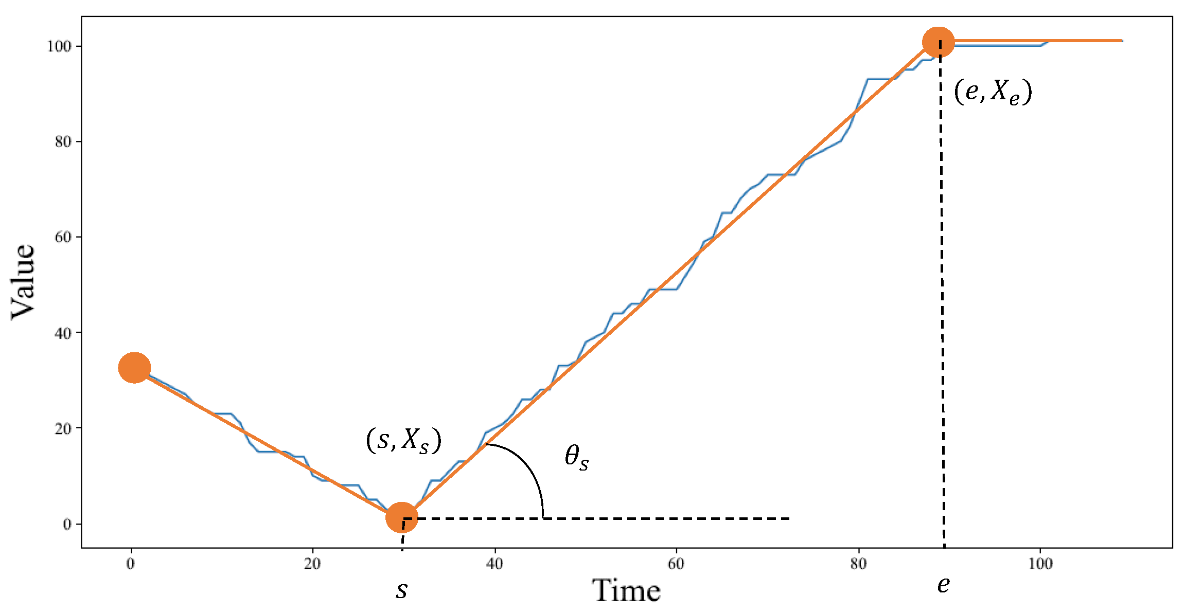
3.2. Enriching ASAR with the Slope Information

While choosing the optimal endpoints from the raw time series to form the new representation, the slopes of the segments are lost (i.e., a segment is a line in the raw time series which connects two endpoints). The slopes can provide very useful information about the local trends. For example, one of the drawbacks of DTW is that it compares the similarity between two instances based only on their magnitude and neglects the trend information. Hence, it may match two instances with the similar values but different trends. Figure 2 shows four different possible scenarios of trends for different instances that have the same value (50, for example). While DTW is searching for the best match, any two of these instances will be considered a perfect match, and the distance between them will be 0. However, it can be noticed that they are different, and a measure that can take their trend into account is required.

Inspired by the BSD method [32], to overcome this drawback, we have modified ASAR to contain the slope information of the original local trends by adding the angle between the horizontal line and the segments to the new representation, see Figure 3. Therefore, we modify Equation (1) as follows:

$$R=\{(R_1,{\theta }_1),(R_2,{\theta }_2),...,(R_k,{\theta }_k)\}$$

(5)

where $\theta$ is the angle between the horizontal line and the line connecting the two endpoints in the raw time series and can be calculated as follows.

$${\theta }_s=arctan\left(\frac{X_e-X_s}{e-s}\right)$$

(6)

where s is the starting point of the line, and e is the endpoint of this line which is found using Equation (4).

By adding this information, the modified representation will contain more information about the shape of the time series by including the information of the slopes of the local trends. In the next subsection, our novel distance measure will be presented, tailored to contain more information about the original shape of the time series.

3.3. Adaptive Simulated Annealing Representation Based Distance Measure (ASAR-Distance)

As previously mentioned, a novel distance measure is proposed in this paper, which aims to satisfy two main objectives: to decrease the dimensionality of the data (enhancing the computation efficiency to speed up the machine learning and data mining algorithms of smart city services) and to increase the accuracy of the distance measures by including more information about the shape of the time series.

Considering two time series ($R^1$) and ($R^2$) (in their adapted ASAR representation), we propose to measure the distance between two points (for instance, i and j) by combining the Manhattan distance and the cosine distance (which makes comparisons based on the slopes) to take into consideration both magnitude and trend:

$$D(R_i^1,R_j^2)=|R_i^1-R_j^2|+(1-cos\left({\theta }_{i,j}\right))$$

(7)

where i and j are the time stamps of the two points, and ${\theta }_{i,j}$ is the angle between $R_i^1$ trend and $R_j^2$ trend (i.e, $|{\theta }_i^1-{\theta }_j^2|$). However, by using this distance definition, only the right trend (future trend) comparison is taken into account, while there are four possible trends changing at a particular point in the raw time series (i.e., rising–rising trend, falling–falling trend, Peak (rising–falling) trend, and Valley (falling–rising) trend). Therefore, we propose to include the previous trend information as well to compare the trend status of the target points by modifying the previous equation as follows:

$$D(R_i^1,R_j^2)=|R_i^1-R_j^2|+(1-cos\left({\theta }_{i,j}\right))+(1-cos\left({\theta }_{i-1,j-1}\right))$$

(8)

By using this definition, the slope information (the local trend information) can be taken into account more precisely as it can compare the four possible trends that a point may lie in. In addition, this measure is combined with the DTW elastic distance measure to find the optimal points’ matching by discovering the optimal path between the two time series.

For the optimal alignment (optimal path) between the two time series, the path that achieves the minimum total cumulative distance should be found, which can be done using dynamic programming as follows:

$$g(R_i^1,R_j^2)=D(R_i^1,R_j^2)+min\left\{\begin{array}{c}g(R_i^1,R_{j-1}^2)\hfill \\ g(R_{i-1}^1,R_{j-1}^2)\hfill \\ g(R_{i-1}^1,R_j^2)\hfill \end{array}\right.$$

(9)

where $D(R_i^1,R_j^2)$ can be computed using Equation (8), which computes the distance between two particular points, and the result (g) represents the ASAR-Distance value. In the next section, the designed experiments and their results are presented to show the effectiveness of using the novel ASAR-Distance to support and speed up the data-based smart city services.

4. Experimental Results and Discussion

In this section, a validation experiment is designed and applied to evaluate the efficiency of the proposed distance method in measuring the dissimilarity between time series and speeding up the data-based smart city applications. ASAR-Distance is compared with the Euclidean and DTW distance methods in two different representation forms, raw time series and ASAR representation. Since direct comparing of distance methods is impossible as no particular information can be extracted from the measure, time series classification and clustering are employed in this paper to compare the distance methods’ ability to measure the time series similarity in shape.

4.1. Assessment Algorithms

Two machine learning methods are applied in this paper to evaluate ASAR-Distance efficiency. The methods are chosen to have a high dependence on the utilized distance method. The first method is the well-known K Nearest Neighbor (K-NN) for classification, while the second is hierarchical clustering.

4.1.1. One Nearest Neighbor Classification (1-NN)

The tested time series is classified using the classes of the closest k time series in K Nearest Neighbor (K-NN) classification [35]. To put it in another way, the method examines the classes of the nearest k time series (using a similarity measure) and uses a majority vote to forecast the tested time series class. Because classification is not the primary goal of this research, the One Nearest Neighbor (1-NN) approach was chosen as the most basic, clear, and conventional way to examine the similarity between time series. Furthermore, it gives a more fair comparison because it does not require parameter adjustment, resulting in impartial findings. We employ half of the dataset under investigation as a training dataset and half as a testing dataset.

4.1.2. Hierarchical Clustering

Hierarchical clustering is a cluster analysis method that aims to create a hierarchy of clusters [36]. There are typically two types of hierarchical clustering: agglomerative and divisive. The agglomerative technique is a “bottom-up” solution in which each time series starts as a single cluster and is combined with cluster pairings to form the hierarchy. The divisive technique is a “top-down” solution in which all time series (altogether) start as a single cluster and are iteratively separated as one progresses down the hierarchy. Agglomerative clustering is faster than divisive, so it has been used in this paper to test the ASAR-Distance efficiency.

4.2. Assessment Criteria

In this study, the F-measure (or F-score) [37] is utilized to compare the classification and clustering outcomes for the ASAR-Distance and the competing methods. It is an accuracy metric calculated by the precision and recall of the test. The precision explains the correct positive predictions out of all positive predictions, while the recall shows the missed positive predictions. The precision is calculated by dividing the number of true predicted positives by the total number of predicted positives. The recall (i.e., sensitivity) is calculated by dividing the number of true predicted positives by the number of real positives. As neither precision nor recall, by themselves, express the entire performance effectiveness, F-Measure combines precision and recall into a single measure that captures both features. The F-measure is defined as follows:

$$F-measure=\frac{2·Precision·Recall}{Precision+Recall}=\frac{TP}{TP+\frac{1}{2}(FP+FN)}$$

(10)

where $TP$ (true positive) is the number of true predicted positives, $FP$ (false positive) is the number of false predicted positives, and $FN$ (false negative) is the number of false predicted negatives.

4.3. Dataset Description

In this study, the UCR Time Series Classification Archive [38] is used to assess the proposed distance method. The data in the repository is z-normalized and comes from a range of domains, giving time series shape diversity. The experiment in this study was run on 11 different datasets. The datasets vary in length and have a range of characteristics. In addition, the datasets have been chosen to be connected to the smart city services. Therefore, datasets of the types: sensor, image, and motion were chosen as they are in the main interest of the smart city applications. However, some datasets were chosen to be not connected to the smart cities to show the ability of the method to measure the distance in other types of time series as well (such as the WormsTwoClass and the Yoga datasets). The UCR repository contains two sets of data: training and testing. We chose the testing set for this experiment because of its larger size so we can evaluate the ability of the proposed method to speed up time series processing in smart cities where big data is available, and to deliver more robust findings. The dataset information utilized in the experiment is shown in

Table 1. The selected datasets from the UCR archive.

Name	Type	Dataset Size	Time Series Length	Number of Classes
HandOutlines	Image	1000	2709	2
StarLightCurves	Sensor	1000	1024	3
Lightning2	Sensor	60	637	2
OSULeaf	Image	200	427	6
WormsTwoClass	Motion	180	900	2
Yoga	Image	1000	426	2
Trace	Sensor	100	275	4
Car	Sensor	60	577	4
CricketX	Motion	390	300	12
InlineSkate	Motion	550	1882	7
UWaveGestureLibraryAll	Motion	1500	945	8

. We chose datasets with diverse time series lengths (short, medium, and long), types, and shapes to evaluate ASAR-Distance’s ability to handle various data forms.

4.4. Effectiveness Evaluation

Euclidean, DTW, and ASAR-Distance are parameter-free methods. However, ASAR needs parameters tuning to create the representation of the time series. As ASAR is not the main focus of this paper, we refer the readers to the paper where ASAR was initially introduced for the details and explanation of its parameter tuning [19].

Three separate evaluations are carried out in this study. We employ 1-NN classification and hierarchical clustering to evaluate ASAR-Distance’s effectiveness in measuring the dissimilarity in shape. Moreover, the effectiveness of ASAR-Distance in supporting rapid data mining operations in smart cities is demonstrated by comparing the time needed to perform classification and clustering tasks using the ASAR-Distance and the competing methods in the case of using the raw time series and the ASAR form. Because 1-NN classification and hierarchical clustering are not the primary goals of this paper, we compute the relative F-measure outcomes by using the different distance methods taking the Euclidean distance on the raw time series as a baseline. This allows us to examine how successful a distance method is compared to using the time series in its raw form with the Euclidean distance. The F-measure relative results for the 1-NN classification are shown in

Table 2. F-measure relative results for 1-NN classification.

Dataset	Raw Time Series		ASAR Form
	Euclidean	DTW	Euclidean	DTW	ASAR-Distance
HandOutlines	1.00	0.99	1.01	1.00	1.02
StarLightCurves	1.00	1.02	1.02	1.01	0.97
Lightning2	1.00	0.88	0.80	0.91	1.04
OSULeaf	1.00	0.97	0.76	0.83	0.93
WormsTwoClass	1.00	0.91	1.02	1.06	1.06
yoga	1.00	1.01	0.84	0.85	0.87
Trace	1.00	0.97	1.19	1.30	1.30
Car	1.00	1.08	1.08	0.93	0.93
CricketX	1.00	1.08	0.84	0.84	0.84
InlineSkate	1.00	0.96	1.06	1.06	1.12
UWaveGestureLibraryAll	1.00	1.01	0.94	0.96	1.00
Average	1.00	0.99	0.96	0.98	1.01

.

Table 3. F-measure relative results for hierarchical clustering.

Dataset	Raw Time Series		ASAR Form
	Euclidean	DTW	Euclidean	DTW	ASAR-Distance
HandOutlines	1.00	1.00	1.00	1.10	1.50
StarLightCurves	1.00	1.04	1.77	1.77	1.70
Lightning2	1.00	1.02	0.84	0.84	1.14
OSULeaf	1.00	0.97	1.12	1.12	1.15
WormsTwoClass	1.00	0.96	1.02	1.04	0.94
yoga	1.00	1.05	1.05	1.12	1.14
Trace	1.00	1.00	1.00	1.00	1.00
Car	1.00	1.00	0.95	0.60	0.60
CricketX	1.00	1.00	1.21	1.25	1.92
InlineSkate	1.00	1.02	1.00	1.00	1.11
UWaveGestureLibraryAll	1.00	1.02	0.95	0.45	1.08
Average	1.00	1.01	1.08	1.03	1.21

, on the other hand, displays the F-measure relative outcomes for the hierarchical clustering task. Among the competing approaches, ASAR-Distance has performed the best. It boosted the accuracy of clustering by 21%.

As previously mentioned, lowering the dimension of the raw time series data results in faster data processing. This can contribute to handling the high computational complexity when using the elastic measures. The runtime needed to finish each experiment was calculated to compare the speed of these methods. The experiments in this paper have been conducted on a platform with an QEMU Virtual CPU with clock speeds at 2.5 and 2.19 GHz with 12 GB RAM, running Windows 10 (64-bit). Python programming language was used to implement and test all the methods. Figure 4 and Figure 5 show the run time of each machine learning task on this platform. We have separated this comparison into two figures, one by using the Euclidean distance and one by using the elastic measures (i.e., the DTW distance and ASAR-Distance). This separation has been done to show clear figures as the time needed in the case of the Euclidean is much lower than for the elastic measures (i.e., the y-axis values are from different ranges). Furthermore, the numerical results for the runtime are shown in

Table 4. Summary of classification and clustering runtimes (in seconds).

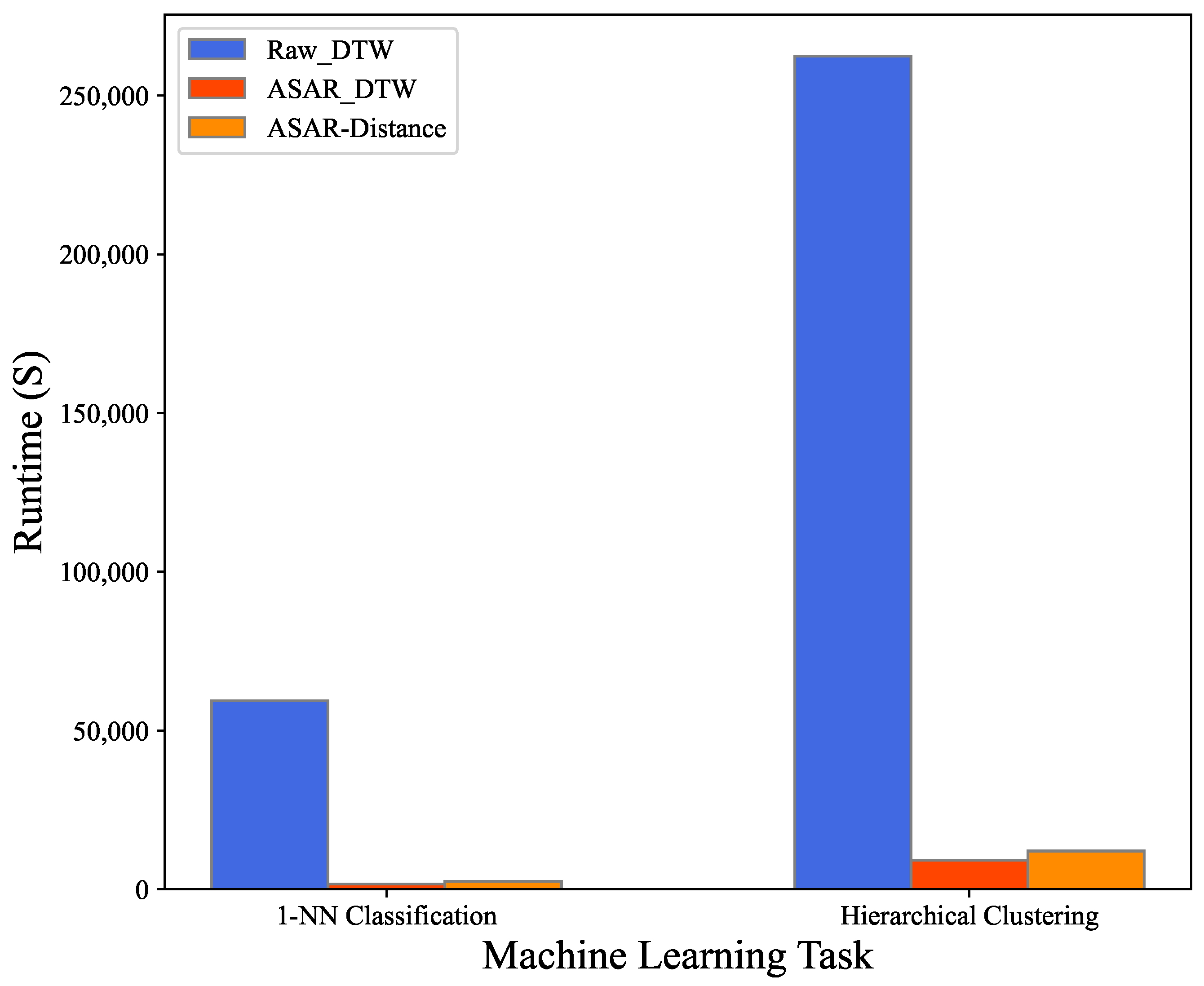
Machine Learning Task	Raw Time Series		ASAR Form
	Euclidean	DTW	Euclidean	DTW	ASAR-Distance
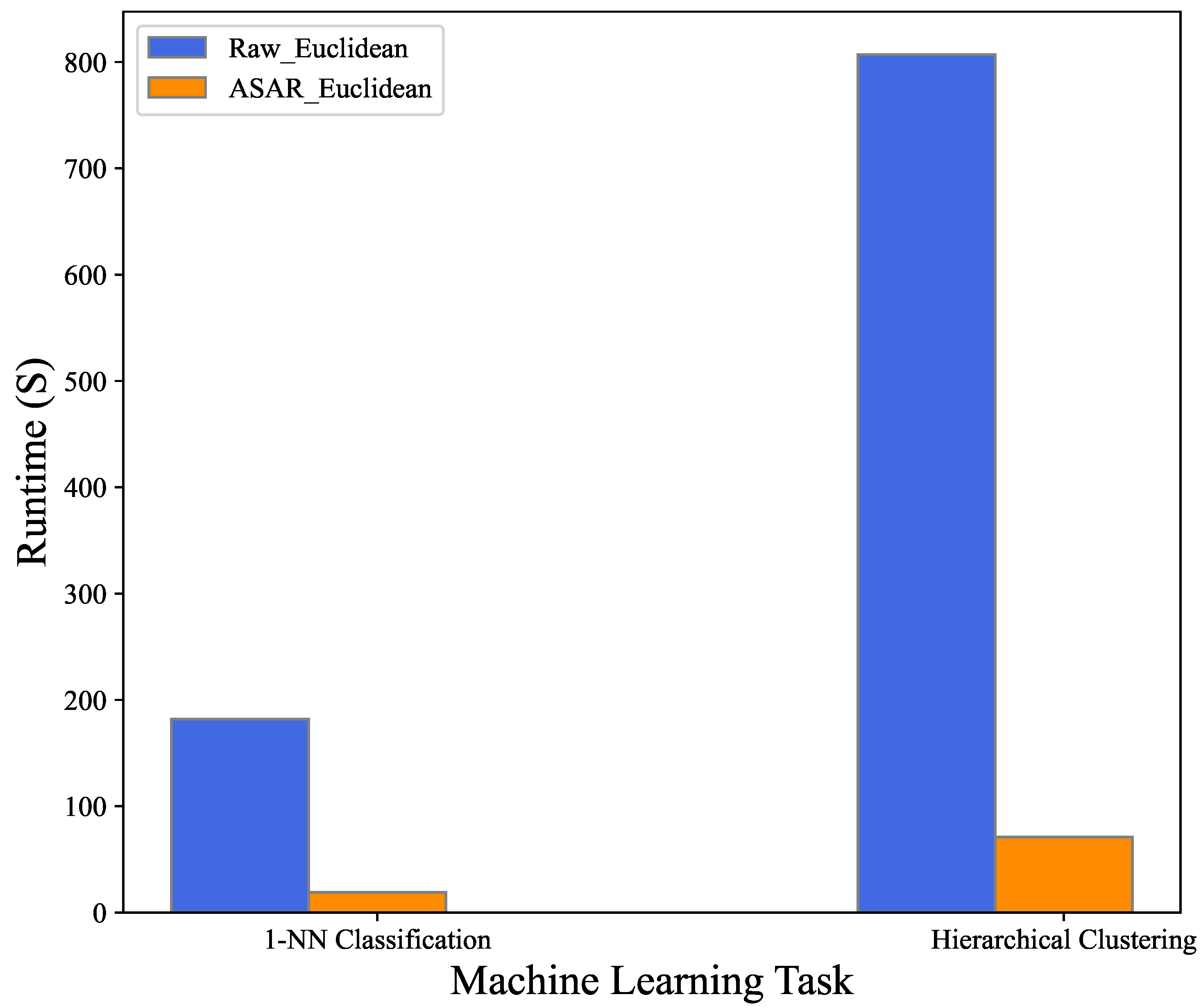
1-NN Classification	182	59,439	19	1642	2556
Hierarchical Clustering	807	262,376	71	9217	12,081

.

4.5. Results Discussion

Table 2 shows that by using the proposed measure, the 1-NN classification becomes more precise by an average of 1% compared to the baseline, which is the Euclidean distance when using the raw time series. However, some loss in accuracy happened when using the ASAR representation with the Euclidean and DTW distance measures (accuracy was still high, which means that the time series information has been preserved). On the other hand, ASAR-Distance has shown superiority among the competing methods, where it has enhanced the hierarchical clustering accuracy by an average of 21%. Even when using the ASAR representation with the Euclidean and DTW distance measures, the accuracy has increased by an average of 8% and 3%, respectively.

Regarding the processing time, the main objective of this paper, ASAR again shows superiority by lowering the dimension of the time series. Figure 4 shows a comparison between using the raw time series and the ASAR form to apply the machine learning tasks with the Euclidean distance. It can be seen that the runtime for the ASAR form is much lower than for the raw time series. In Figure 5, the same comparison can be seen, but with the elastic measures (i.e., DTW and the ASAR-Distance measures). The figure shows the long processing time needed when utilizing the time series in its raw form. This time has been decreased remarkably by lowering the dimension of the data. The best performance was obtained by using the ASAR form with the DTW. Still, ASAR-Distance has shown a very close runtime, making it much faster than using the raw time series with the DTW. A numerical comparison is also shown in Table 4.

The results above confirm that the ASAR representation and its variant proposed in this paper can decrease the time series dimensionality and preserve the shape while keeping all the relevant information about the local trends. In addition, it proves that the ASAR-Distance can measure the similarity better than the competing methods, with an average of 1% in the case of 1-NN classification and an average of 21% in the case of hierarchical clustering. This benefit of high accuracy in measuring the similarity is obtained with relatively low computational cost. Researchers have preferred the DTW measure over the Euclidean distance in many machine learning applications for its ability to handle the local time-shifting even with the inherited long runtime. The proposed distance measure in this paper introduces a solution for smart city applications to overcome this issue, making it possible to use an elastic measure that can handle the local time-shifting and decrease the runtime. The results have shown that the ASAR-Distance measure does not only reduce the runtime of using an elastic measure but increases the accuracy of measuring the similarity by reading more information about the local trends in the raw time series.

5. Conclusions

In this paper, a novel elastic distance measure, ASAR-Distance, has been proposed. ASAR-Distance aims to overcome the limitations of handling the local time shifting, reading the local trends information precisely, and the inherited high computational complexity of the elastic distance measures. A modified version of the ASAR approach has been introduced by adding the slope information for each segment. This information can help compare the instances in two time series by comparing based on the trends in addition to comparing based on the magnitude (by combining the Manhattan, Cosine, and Dynamic Time Warping distance measures). The experimental results have shown that the ASAR-Distance has fulfilled its objective and was able to overcome these limitations. They show that ASAR-Distance introduces a solution for using the preferable elastic measures, with higher efficiency of measuring the similarity and lower computational cost of applying machine learning tasks, which can speed up the time series processing for smart city applications.

References

- Saqib, M.; Jasra, B.; Moon, A.H. A lightweight three factor authentication framework for IoT based critical applications. J. King Saud Univ. Comput. Inf. Sci. 2021; in press. [Google Scholar] [CrossRef]
- Syed, A.S.; Sierra-Sosa, D.; Kumar, A.; Elmaghraby, A. IoT in smart cities: A survey of technologies, practices and challenges. Smart Cities 2021, 4, 429–475. [Google Scholar] [CrossRef]
- Wu, J.; Guo, S.; Li, J.; Zeng, D. Big data meet green challenges: Greening big data. IEEE Syst. J. 2016, 10, 873–887. [Google Scholar] [CrossRef]
- Wu, J.; Guo, S.; Huang, H.; Liu, W.; Xiang, Y. Information and communications technologies for sustainable development goals: State-of-the-art, needs and perspectives. IEEE Commun. Surv. Tutor. 2018, 20, 2389–2406. [Google Scholar] [CrossRef] [Green Version]
- Doan, Q.T.; Kayes, A.; Rahayu, W.; Nguyen, K. Integration of iot streaming data with efficient indexing and storage optimization. IEEE Access 2020, 8, 47456–47467. [Google Scholar] [CrossRef]
- Koubaa, A.; Aldawood, A.; Saeed, B.; Hadid, A.; Ahmed, M.; Saad, A.; Alkhouja, H.; Ammar, A.; Alkanhal, M. Smart Palm: An IoT framework for red palm weevil early detection. Agronomy 2020, 10, 987. [Google Scholar] [CrossRef]
- Kim, H.; Choi, H.; Kang, H.; An, J.; Yeom, S.; Hong, T. A systematic review of the smart energy conservation system: From smart homes to sustainable smart cities. Renew. Sustain. Energy Rev. 2021, 140, 110755. [Google Scholar] [CrossRef]
- Khan, M.M.; Mehnaz, S.; Shaha, A.; Nayem, M.; Bourouis, S. IoT-Based Smart Health Monitoring System for COVID-19 Patients. Comput. Math. Methods Med. 2021, 2021, 8591036. [Google Scholar] [CrossRef]
- Bawaneh, M.; Simon, V. Anomaly detection in smart city traffic based on time series analysis. In Proceedings of the 2019 International Conference on Software, Telecommunications and Computer Networks (SoftCOM), Split, Croatia, 19–21 September 2019; pp. 1–6. [Google Scholar]
- Pardini, K.; Rodrigues, J.J.; Kozlov, S.A.; Kumar, N.; Furtado, V. IoT-based solid waste management solutions: A survey. J. Sens. Actuator Netw. 2019, 8, 5. [Google Scholar] [CrossRef] [Green Version]
- Ali, G.; Ali, T.; Irfan, M.; Draz, U.; Sohail, M.; Glowacz, A.; Sulowicz, M.; Mielnik, R.; Faheem, Z.B.; Martis, C. IoT based smart parking system using deep long short memory network. Electronics 2020, 9, 1696. [Google Scholar] [CrossRef]
- Kaginalkar, A.; Kumar, S.; Gargava, P.; Niyogi, D. Review of urban computing in air quality management as smart city service: An integrated IoT, AI, and cloud technology perspective. Urban Clim. 2021, 39, 100972. [Google Scholar] [CrossRef]
- Ali, M.; Alqahtani, A.; Jones, M.W.; Xie, X. Clustering and classification for time series data in visual analytics: A survey. IEEE Access 2019, 7, 181314–181338. [Google Scholar] [CrossRef]
- Ciaburro, G.; Iannace, G. Machine Learning-Based Algorithms to Knowledge Extraction from Time Series Data: A Review. Data 2021, 6, 55. [Google Scholar] [CrossRef]
- Blázquez-García, A.; Conde, A.; Mori, U.; Lozano, J.A. A review on outlier/anomaly detection in time series data. ACM Comput. Surv. (CSUR) 2021, 54, 1–33. [Google Scholar] [CrossRef]
- Belhadi, A.; Djenouri, Y.; Nørvåg, K.; Ramampiaro, H.; Masseglia, F.; Lin, J.C.W. Space–time series clustering: Algorithms, taxonomy, and case study on urban smart cities. Eng. Appl. Artif. Intell. 2020, 95, 103857. [Google Scholar] [CrossRef]
- Abanda, A.; Mori, U.; Lozano, J.A. A review on distance based time series classification. Data Min. Knowl. Discov. 2019, 33, 378–412. [Google Scholar] [CrossRef] [Green Version]
- Torkamani, S.; Lohweg, V. Survey on time series motif discovery. Wiley Interdiscip. Rev. Data Min. Knowl. Discov. 2017, 7, e1199. [Google Scholar] [CrossRef]
- Bawaneh, M.; Simon, V. A Novel Time Series Representation Approach for Dimensionality Reduction. Infocommun. J. 2022, 14, 44–55. [Google Scholar] [CrossRef]
- Faloutsos, C.; Ranganathan, M.; Manolopoulos, Y. Fast subsequence matching in time-series databases. Acm. Sigmod. Rec. 1994, 23, 419–429. [Google Scholar] [CrossRef] [Green Version]
- Berndt, D.J.; Clifford, J. Using dynamic time warping to find patterns in time series. In KDD Workshop; AAAI Press: Seattle, WA, USA, 1994; Volume 10, pp. 359–370. [Google Scholar]
- Yi, B.K.; Faloutsos, C. Fast time sequence indexing for arbitrary Lp norms. In Proceedings of the 26th International Conference on Very Large Data Bases Cairo (VLDB’00), Cairo, Egypt, 10–14 September 2000; pp. 385–394. [Google Scholar]
- Ahmadi, A.; Karray, F.; Kamel, M.S. Flocking based approach for data clustering. Nat. Comput. 2010, 9, 767–791. [Google Scholar] [CrossRef]
- Vlachos, M.; Kollios, G.; Gunopulos, D. Discovering similar multidimensional trajectories. In Proceedings of the 18th International Conference on Data Engineering, San Jose, CA, USA, 26 February–1 March 2002; pp. 673–684. [Google Scholar]
- Chen, L.; Özsu, M.T.; Oria, V. Robust and fast similarity search for moving object trajectories. In Proceedings of the 2005 ACM SIGMOD International Conference on Management of Data, Baltimore, MA, USA, 14–16 June 2005; pp. 491–502. [Google Scholar]
- Chen, L.; Ng, R. On the marriage of lp-norms and edit distance. In Proceedings of the Thirtieth International Conference on Very Large Data Bases-Volume 30, Toronto, ON, Canada, 31 August–3 September 2004; pp. 792–803. [Google Scholar]
- Chen, Y.; Nascimento, M.A.; Ooi, B.C.; Tung, A.K. Spade: On shape-based pattern detection in streaming time series. In Proceedings of the 2007 IEEE 23rd International Conference on Data Engineering, Istanbul, Turkey, 15–20 April 2007; pp. 786–795. [Google Scholar]
- Lin, J.; Keogh, E.; Lonardi, S.; Chiu, B. A symbolic representation of time series, with implications for streaming algorithms. In Proceedings of the 8th ACM SIGMOD Workshop on Research Issues in Data Mining and Knowledge Discovery, San Diego, CA, USA, 13 June 2003; pp. 2–11. [Google Scholar]
- Lin, J.; Keogh, E.; Wei, L.; Lonardi, S. Experiencing SAX: A novel symbolic representation of time series. Data Min. Knowl. Discov. 2007, 15, 107–144. [Google Scholar] [CrossRef] [Green Version]
- Zhang, M.; Pi, D. A new time series representation model and corresponding similarity measure for fast and accurate similarity detection. IEEE Access 2017, 5, 24503–24519. [Google Scholar] [CrossRef]
- Gullo, F.; Ponti, G.; Tagarelli, A.; Greco, S. A time series representation model for accurate and fast similarity detection. Pattern Recognit. 2009, 42, 2998–3014. [Google Scholar] [CrossRef]
- Kamalzadeh, H.; Ahmadi, A.; Mansour, S. Clustering time-series by a novel slope-based similarity measure considering particle swarm optimization. Appl. Soft Comput. 2020, 96, 106701. [Google Scholar] [CrossRef]
- Kamalzadeh, H.; Ahmadi, A.; Mansour, S. A shape-based adaptive segmentation of time-series using particle swarm optimization. Inf. Syst. 2017, 67, 1–18. [Google Scholar] [CrossRef]
- Kirkpatrick, S.; Gelatt, C.D.; Vecchi, M.P. Optimization by simulated annealing. Science 1983, 220, 671–680. [Google Scholar] [CrossRef]
- Lee, Y.H.; Wei, C.P.; Cheng, T.H.; Yang, C.T. Nearest-neighbor-based approach to time-series classification. Decis. Support Syst. 2012, 53, 207–217. [Google Scholar] [CrossRef]
- Murtagh, F.; Contreras, P. Algorithms for hierarchical clustering: An overview. Wiley Interdiscip. Rev. Data Min. Knowl. Discov. 2012, 2, 86–97. [Google Scholar] [CrossRef]
- Fawcett, T. An introduction to ROC analysis. Pattern Recognit. Lett. 2006, 27, 861–874. [Google Scholar] [CrossRef]
- Dau, H.A.; Keogh, E.; Kamgar, K.; Yeh, C.C.M.; Zhu, Y.; Gharghabi, S.; Ratanamahatana, C.A.; Hu, B.; Begum, N.; Bagnall, A.; et al. The UCR Time Series Classification Archive. 2018. Available online: https://www.cs.ucr.edu/~eamonn/time_series_data_2018/ (accessed on 6 April 2022).