Improvement of Natural Frequency Prediction from Spectrogram of Bone-Conducted Sound by Data Augmentation

Abstract

In this study, the effect of data augmentation on machine learning (ML) models that predict the natural frequency of human long bones from the spectrogram of bone-conducted sound was investigated. Bone-conducted sound was recorded from the tibia of 45 healthy university students using a custom-developed hammering device. Short-Time Fourier Transform (STFT) was applied to the recorded sounds to generate spectrograms, from which six ML models were examined to predict the natural frequency. Ground-truth natural frequency was defined as peak values identified from Fast Fourier Transform (FFT) spectra obtained by recorded waveforms of sounds. Data augmentation was performed by shifting bone-conducted sound waveforms, expanded to 5 levels, i.e., 3-fold (3×) to 11-fold (11×). All models showed improved accuracy by data augmentations compared to the original dataset, with a particularly substantial improvement observed in many models when the dataset was expanded from the original to the 3× level. Among the ML models examined here, DenseNet-121 with 11× data augmentation achieved the lowest MAE and the highest R² (10.00 ± 2.27 Hz; R² = 0.927 ± 0.046), followed by PeleeNet, which is constructed on a lightweight DenseNet architecture, with 7× data augmentation (MAE = 10.37 ± 2.91 Hz, R² = 0.920 ± 0.059).

1. Introduction

Bone mineral density (BMD) measurement is widely used to evaluate bone health. To measure BMD, DXA (Dual-energy X-ray Absorptiometry), QCT (Quantitative Computed Tomography), and QUS (Quantitative Ultrasound) have been widely used. Among these methods, DXA is currently the most commonly used measurement method [1,2]. However, this method is typically applied only to specific populations, such as postmenopausal women and individuals with low bone mass or bone loss [3,4]. Furthermore, it does not accurately identify osteoporosis measures areal BMD, which measures areal density values in grams per square centimeter, not volumetric density [5]. Among all non-vertebral fractures in elderly men and women, the proportions with BMD below the osteoporosis threshold were only 21% and 34% in men and women, respectively, indicating that factors other than BMD are also necessary for predicting fracture risk [6]. On the other hand, CT can measure volumetric BMD; thus, CT discriminates fragility fractures better than DXA [7]. Although CT is more accurate than DXA, it is rarely used for routine examinations due to the radiation dose, cost, and the need for standardized protocols [8]. In contrast, QUS, which is a method for estimating BMD based on the speed at which ultrasound waves travel through bone [9], is safer with more compact measurement equipment that does not require radiation exposure. QUS differs from DXA in its measurement principle, and it has been shown to have a weak correlation with DXA-based BMD (r = 0.35), missing the majority of osteoporotic patients, and may not be a sufficiently reliable screening tool [10]. BMD measurement has several limitations, including the risk of radiation exposure and low reproducibility across measurements. In addition, as BMD does not sufficiently reflect overall bone strength, it is necessary to evaluate overall bone strength, including both bone mineral density and bone quality [11]. Therefore, an accurate and non-radiative measurement method suitable for routine clinical screening is required.

As one approach to bone strength measurement, the impulse response method has been conducted [12,13,14,15,16]. BMD alone does not represent mechanical bone strength, as current BMD measurement methods evaluate bone based on age-related reference values of density rather than directly measuring mechanical properties [16]. The impulse response method enables measurement of the mechanical properties of bone. This method estimates bone strength by applying a weak impact to one end of the bone to generate bone-conducted sound, from which the natural frequency of the bone can be measured.

In previous studies using the impulse response method, experimenters manually applied an impact to the bone, and the natural frequency of the bone-conducted sound was estimated using FFT analysis, requiring both manual measurement and signal analysis. The previous manual method is extremely difficult to maintain accuracy because variability in the natural frequency can occur if the hammering force is not constant. In addition, it was also difficult to identify the natural frequency through signal processing with FFT. Even when using an automated device to measure, specialized expertise was still required in certain situations, such as appropriate subject positioning and interpretation of waveform results [16,17]. The fact that this method requires a well-trained experimenter is considered as one reason why this method may not be widely used as a screening tool. To address this limitation, a machine learning (ML) model for predicting the natural frequency is being developed, which employs time-frequency analysis to obtain spectrogram images from bone-conducted sound, from which the natural frequency is estimated using Convolutional Neural Network (CNN)-based image analysis [18]. A similar approach has already been applied to the detection of internal defects in concrete using hammering-sound tests. In conventional peak frequency methods with FFT analysis, identifying defects required user expertise and subjective judgment [19]. In concrete hammering tests, FFT-based frequency analysis has been conventionally used; however, it is difficult to identify defects from the spectra because their interpretation required expertise [20]. By applying STFT-based spectrograms as inputs to CNN models, defect classification has been demonstrated without relying on expert judgment [19,20]. This indicates that this approach can overcome the challenges that require specialized expertise. Since the impulse response method for bone shares the same measurement principle of impact-induced vibration analysis, a similar transition from FFT-based analysis to STFT-based spectrogram input for CNN is proposed in the present study. Our previous research reported that the proposed method can visualize time transition and frequency in bone-conducted sound, enabling a more comprehensive analysis than the conventional method [18]. Furthermore, it suggested that in applying a ML model, there is a possibility of preventing measurement errors by automatically and prompting re-measurement when the analysis of bone-conducted sound is inaccurate. To establish the proposed method as a practical screening tool using the impulse response method, the ML model should reproduce natural frequencies of conventional FFT analysis. Since a wide variety of CNN architectures are available, it is necessary to explore the models for the predictions of the natural frequency from spectrograms of bone-conducted sound. In general, large amounts of datasets are mandatory to develop a ML model. However, collecting enough of bone-conducted sound data to develop it requires considerable cost and effort. To support such difficulty, data augmentation is used as an effective technique to improve the generalization performance of models and reduce the dependence on large datasets [21]. In our previous study [18], only ResNet was used and the effect of data augmentation on the prediction accuracy was not examined; in this study, the effect of data augmentation by time-shifting the waveforms on the prediction accuracy of the natural frequency of bone-conducted sound is investigated by examining six ML models and changing the augmentation levels.

2. Methods

2.1. Dataset

The dataset used in this study was obtained by measuring the bone-conducted sound of the tibia in 45 healthy male and female university students using a custom-developed hammering device (17 males and 28 females; mean age: 20.36 ± 1.53 years; no fracture present in the measured tibia at the time of measurement). The tibia was selected as the target bone in this study, since it is a long bone with relatively thin overlying soft tissue at the medial surface, which facilitates non-invasive hammering measurements.

The principle of the impulse response method is to evaluate mechanical properties of bone by analyzing vibrations generated by a strike. More specifically, this method models the vibration of a long bone as that of a beam with both ends free, based on the transverse vibration of beams in Timoshenko beam theory, and estimates them from its natural frequency [13,22].

Equation (1) is the formula for calculating the natural frequency from the equation of motion for transverse vibration of beams.

$$\begin{array}{c}{f}_n={\displaystyle \frac{{\omega }_n}{2\pi }}={\displaystyle \frac{{{\lambda }_n}^2}{2\pi L^2}}\sqrt{{\displaystyle \frac{E{I}_Z}{\rho S}}}.\end{array}$$

(1)

Here, $f_n$ is the natural frequency, $n$ the vibrational mode number, $E$ the Young’s modulus, $I_z$ the moment of inertia, $L$ the length of beam (the bone length), ${\lambda }_n$ the vibrational mode, $\rho$ the mass density (the bone mineral density), and $S$ the cross-sectional area of the beam. From this equation, we can obtain

$$\begin{array}{c}{\displaystyle \frac{{\rm E}}{\rho }}={\displaystyle \frac{4{\pi }^{2}S}{{{\lambda }_n}^4{I}_Z}}{f_n}^2{L}^4.\end{array}$$

(2)

The bone strength index is defined as $E/\rho$, the left-hand side of Equation (2). Here, by assuming that $I_z$, ${\lambda }_n$, $S$ are constants, from the observed values of ${f_n}^2{L}^4$, we can evaluate the bone strength index, $E/\rho$.

To get bone-conducted sound waveforms, an acceleration sensor (GSS-4SC, SENSATEC, Kyoto, Japan) was attached to the medial condyle of the right tibia, and five consecutive hammer strikes were applied perpendicular to the medial malleolus of the right foot. The sampling frequency was set to 11,025 Hz. A total of 225 bone-conducted sound recordings obtained from this measurement were used in this study.

2.2. Analysis Methods for Natural Frequency of Bone-Conducted Sound

The obtained bone-conducted sound was analyzed using both FFT and STFT. It is necessary to account for such vibrational mode and soft tissue effects in the evaluation of bone-conducted sound [13,16]. The natural frequency of the first vibrational mode of the wet tibia in the sagittal plane has been reported to be 360 Hz [13], the natural frequency of non-fractured tibia measured by impulse response method has been reported to be approximately 300–400 Hz in clinical research [23], and the frequency of the tibialis anterior has been reported to be 16.3–62.6 Hz [24]. To remove these influences, a bandpass filter of 200–500 Hz was applied for waveform processing. The FFT conditions were set as follows: FFT size was 1024 and frequency resolution was 10.8 Hz. The STFT conditions were set as follows: FFT size was 512, window length 512, hop length 128 (1/4), time resolution 11.6 ms, and frequency resolution 21.6 Hz. Hanning window was applied in both cases.

Spectrograms were obtained by applying Short-Time Fourier Transform (STFT) to the bone-conducted sound and were converted to images of 224 × 224 × 3 pixels. The ground-truth labels for the natural frequency were defined as the peak frequency manually identified using FFT analysis of each sound. Natural frequencies were predicted by the model from the input spectrograms.

2.3. ML Models

Six ML models were examined in this study: AlexNet [25], VGG-16 [26], ResNet-18 [27], DenseNet-121 [28], PeleeNet, a lightweight variant of DenseNet with fewer layers [29], and EfficientNet-B0 [30]; parameter counts are summarized in

Table 1. ML models and number of parameters.

Model	Parameters
AlexNet	71,922,433
VGG-16	134,264,641
ResNet-18	11,449,281
DenseNet-121	7,562,817
PeleeNet	2,817,841
EfficientNet-B0	4,050,852

. As the number of parameters increases, the complexity of the model increases.

2.4. Data Augmentation

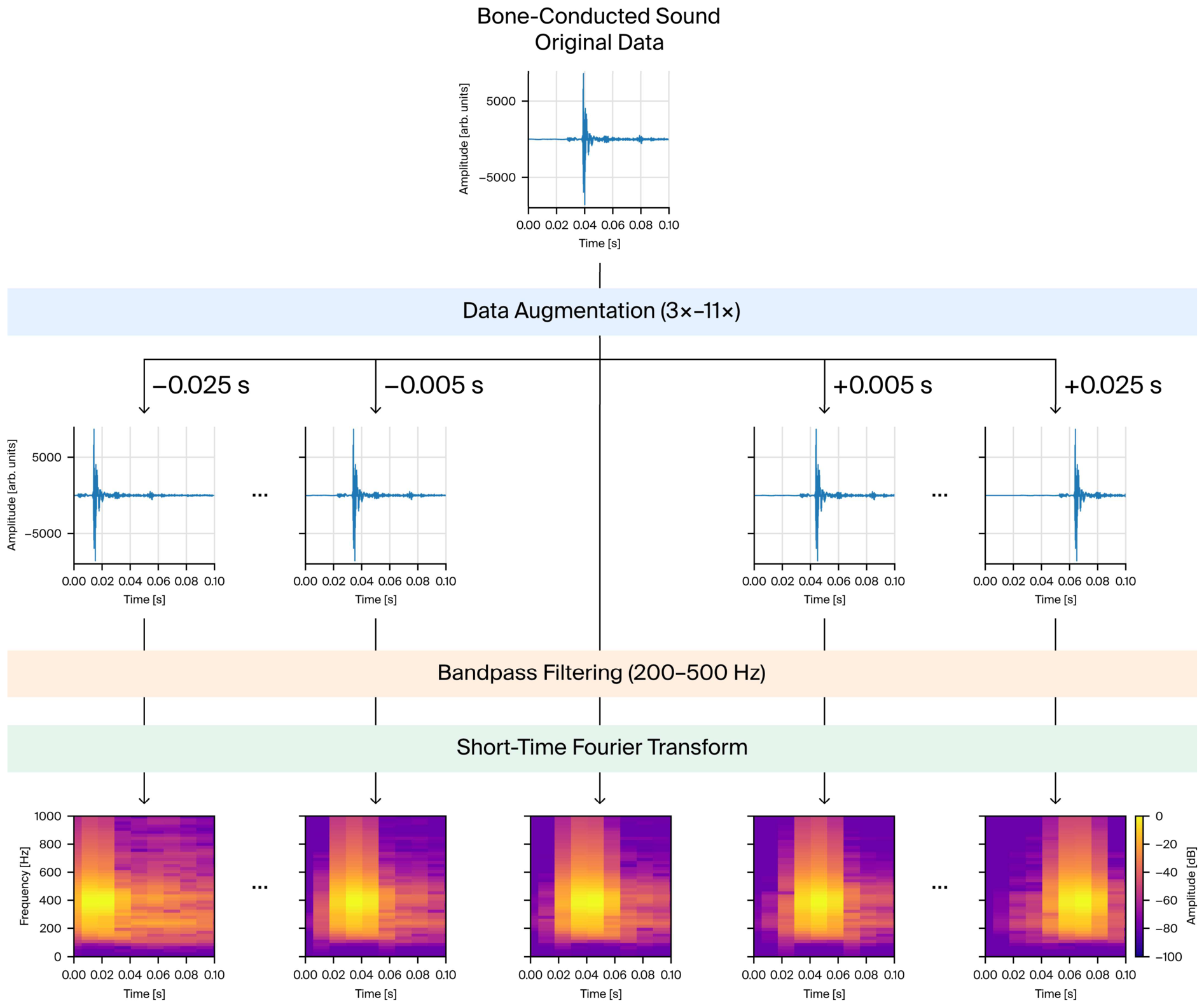
In this study, the bone-conducted sound waveforms were shifted forward and backward in time prior to bandpass filtering to generate additional spectrograms, thereby augmenting the training dataset. Here, only the above-mentioned time-shift method was used for data augmentation to minimize the influence of bandpass filtering as in our previous study [18]. The training dataset was expanded to N times its original size (N-fold: N×), where the shift step was 0.005 s per increment. Five augmentation levels were evaluated: 3× (0, ±0.005 s), 5× (0, ±0.005, ±0.010 s), 7× (0, ±0.005, ±0.010, ±0.015 s), 9× (0, ±0.005, ±0.010, ±0.015, ±0.020 s), and 11× (0, ±0.005, ±0.010, ±0.015, ±0.020, ±0.025 s). Data augmentation procedure is schematically shown in Figure 1, which was applied only to the training set within each fold of cross-validation.

2.5. Training and Evaluation Methods for ML Models

The training conditions for the ML models in this study are shown in

Table 2. Training conditions of ML models.

Hyperparameters	Conditions
Input size	224 × 224 × 3
Epochs	50
Optimizer	Adam [32]
Loss function	MSE (mean squared error)
Batch size	ReLU [33]
Initial learning rate	0.001

. To prevent stagnation in model learning, ReduceLROnPlateau was employed to adjust the learning rate when training progress stalled. This function automatically reduces the learning rate by a factor of 0.5 [31]. The learning rate was automatically halved when the validation loss did not improve for 5 consecutive epochs.

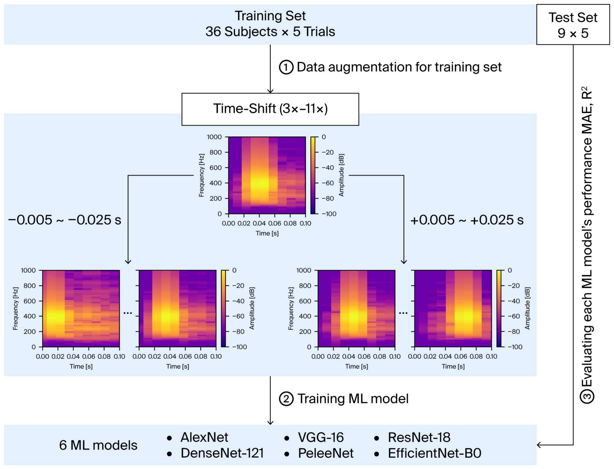
To evaluate model performance while preventing data from the same participant appearing in both the training and test sets, 5-fold cross-validation was performed at the subject level (Group K-Fold), in which all recordings from the same participant were assigned exclusively to either the training or test set. Because data from the same subject are correlated, including them in both sets increases the risk of overfitting [34]. The 45 subjects were divided into five folds, resulting in a training set of 180 recordings (36 subjects × 5 recordings) per fold. The mean MAE (Mean Absolute Error) and mean R² across the five validation folds were calculated (Figure 2). All models were trained from scratch without pre-trained weights, since ImageNet images differ substantially from bone-conducted sound spectrogram.

3. Results and Discussion

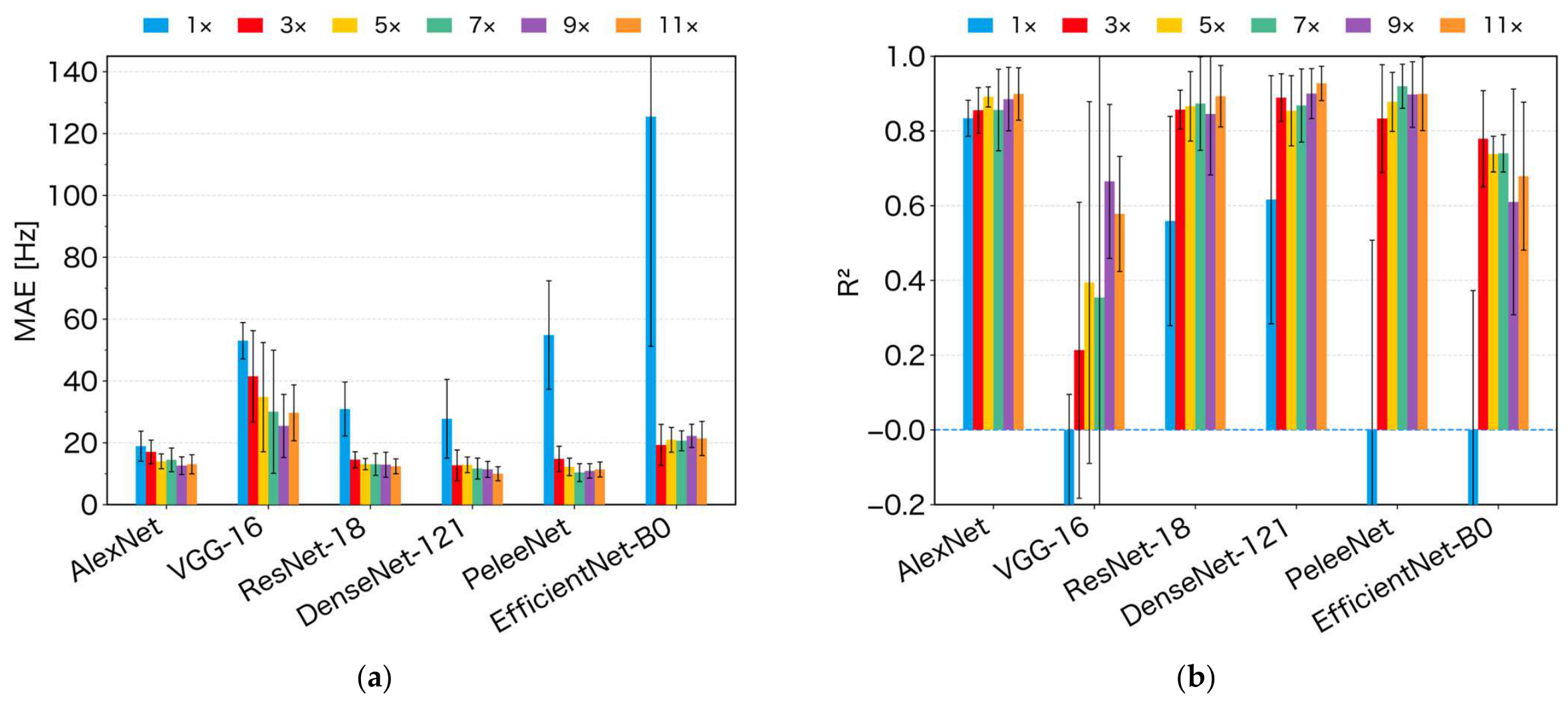
Figure 3a,b shows the mean MAE and the mean R², respectively, of the validation data from the cross-validation for 1× to 11× data augmentation. A tendency for MAE to decrease and for R² to increase as the level of data augmentation increased was observed, indicating an improvement in prediction accuracy.

Table 3. Top five models ranked by MAE.

Rank	Model	Fold	MAE ± SD (Hz)
1	DenseNet-121	11	10.00 ± 2.27
2	PeleeNet	7	10.37 ± 2.91
3	PeleeNet	9	10.91 ± 2.36
4	PeleeNet	11	11.34 ± 2.44
5	DenseNet-121	9	11.38 ± 2.58

shows the results for the top five models ranked in ascending order of MAE. The model with the lowest MAE and the highest R² was DenseNet-121 with 11× augmentation, yielding an MAE of 10.00 ± 2.27 Hz, and R² = 0.927 ± 0.046. This was followed by PeleeNet with 7× augmentation (MAE = 10.37 ± 2.91 Hz, R² = 0.920 ± 0.059). Those with the third, fourth and the fifth lowest MAEs were PeleeNet with 9× and 11×, and DenseNet-121 with 9× augmentations, respectively.

DenseNet-121 with 11× augmentation achieved the lowest MAE among the models. The MAE of 10.00 Hz corresponds to 2.69% of the mean natural frequency (371.87 Hz), while PeleeNet with 7× augmentation achieved a comparable MAE of 10.37 Hz (2.79%). This indicates that the ML-based automated prediction reproduces natural frequencies by the FFT analysis used in previous studies using the impulse response method. While only ResNet-18 was used in the previous study [18], here we examined six ML models. Among the models examined here and included in the previous study, the DenseNet architecture (DenseNet-121 and PeleeNet) achieved relatively higher prediction accuracy than the other models. This suggested that the architectures of these two may be well-suited for natural frequency prediction from spectrograms of bone-conducted sound.

DenseNet-121 with 11× augmentation shows lower MAE and higher R² than PeleeNet with 7× augmentation. However, there was no significant difference between the top two models when the one-sided Wilcoxon signed-rank test was used (p = 0.3125). This indicates that PeleeNet can achieve the prediction accuracy as good as DenseNet-121, though PeleeNet had approximately one-third the number of parameters.

As shown in Figure 3a, increasing the level of data augmentation generally improved prediction accuracy. In particular, for ResNet, DenseNet, PeleeNet, and EfficientNetB0, the statistical analysis using the one-sided Wilcoxon signed-rank test showed that a statistically significant improvement in accuracy was confirmed when data augmentation was applied to 3× compared with the original dataset (1×) (p < 0.05). These results suggest that even with a small number of datasets, it is possible to develop a more accurate ML model by data augmentation. This indicates that it may be possible to develop the ML model with higher accuracy by using data augmentation, even if data collection is difficult. However, in VGG-16, PeleeNet, and EfficientNet-B0, MAE was increased and R² was decreased from 9× to 11×, from 7× to 9×, and from 7× to 9×, respectively. This suggests that excessive augmentation may introduce redundant or less informative samples, leading to model saturation [35]. Papasratorn et al. [36] reported that the highest accuracy was achieved at 10-fold augmentation and performance declined at higher augmentation factors in all deep learning models for automated recognition of contiguity between the mandibular third molar and inferior alveolar canal, using panoramic radiographs. From the observation of a similar trend in the present study, the following hypothesis appears: an optimal level of data augmentation exists in image analysis of spectrogram-obtained bone-conducted sound. To verify this hypothesis, it is necessary to conduct a validation process using visualization of augmented samples or feature-space analysis.

One limitation of this study is that augmentation levels were evaluated only up to 11×, and the optimal fold of data augmentation differed among the models. Another limitation is that although Group K-Fold cross-validation was employed here, there is a lack of an independent external validation dataset, since we have only small numbers in the dataset, i.e., 45 subjects who are healthy university students in the present study. Thus, the reported method with the current dataset is limited to the application only for healthy young adults. Finally, the dataset with the excessive data augmentation may possibly produce redundant samples. To reveal this, feature-space analysis can be effective to verify the similarity between the original dataset and augmented samples.

Future development is directed toward an edge device that can automatically perform the entire process from measurement to analysis on site. To achieve this, it is necessary to develop a lightweight CNN model that can operate on small devices with limited computational resources, such as a Raspberry Pi, while enabling real-time analysis on site [31,37]. CNN models with a high number of parameters, such as VGG-16, require substantial computational resources, making them impractical for deployment on resource-constrained edge devices [37]. Therefore, considering the model for practical use, the six ML models developed using Keras frameworks were converted to ONNX formats [38], and the inference time was measured using an Apple M5 MacBookPro (10-core CPU, 10-core GPU, 16-core Neural Engine, 24 GB RAM). For models developed using 11× augmentation, the time per image was calculated from the time from nine subjects.

Table 4. Computational costs of the ML models for training.

Model	Training Time (s)	Peak GPU Memory Usage (GB)	FLOPs
AlexNet	881.7	2.44	2.54 G
VGG-16	3887.5	7.29	30.95 G
ResNet-18	1015.6	1.43	3.64 G
DenseNet-121	7111.7	7.51	5.70 G
PeleeNet	4827.8	1.71	1.03 G
EfficientNet-B0	3446.9	4.23	0.80 G

shows the computational costs of the ML models for training with 11× augmentation, and

Table 5. Inference time and model size of each model.

Model	Inference Time (One/ms)	Model Size (MB)
AlexNet	8.23	274.36
VGG-16	57.49	512.19
ResNet-18	17.32	43.63
DenseNet-121	17.10	28.61
PeleeNet	4.62	10.84
EfficientNet-B0	12.64	15.34

shows the measured inference time and model size for each model after the models were converted. This demonstrated that PeleeNet had the smallest model size and the faster inference time. Considering prediction accuracy, the cost of calculation, and inference time, PeleeNet, which offers a well-balanced combination of being a lightweight model and having higher prediction accuracy, may be considered to be a promising candidate for an edge device application.

From these findings, future work should explore a wider range of augmentation levels to determine the optimal fold for each model and identify the most suitable model according to the available computational resources.

4. Conclusions

In this study, the effect of data augmentation has been investigated to improve prediction accuracy for the natural frequency of human long bones from spectrograms of bone-conducted sound. Six ML models were examined, and the fold of data augmentation was set at five levels from 3× to 11×. The investigation of data augmentation effects revealed that all models achieved higher prediction accuracy when the data augmentation was applied than with the original (1×) dataset. Among these, an improvement in accuracy was observed in many models when the dataset was extended from 1× to 3× augmentation. It should be noted here that the current data augmentation method is based upon the time-shift of the waveforms of bone-conducted sound, which can produce slightly different data; however, these profiles are similar, yielding improvements regarding the data representation capabilities in machine learning. Considering the examination results on augmentation levels, current time-shift-type augmentation worked well. In addition, it was suggested that it is possible for ML models to improve the prediction accuracy by applying data augmentation even with a small dataset of bone-conducted sounds. Furthermore, PeleeNet, which has the smaller number of parameters among six ML models, demonstrated prediction accuracy as good as the models with more complex architectures. Based on the results of prediction accuracy, inference time, and computational costs, it is suggested that a lightweight model such as PeleeNet can achieve higher prediction accuracy by combining a lightweight model with data augmentation techniques in the task of predicting natural frequencies from bone-conducted sounds. Future work will focus on identifying the model with higher prediction accuracy and the optimal level of data augmentation for practical applications. Additional verifications are required to use (1) recently developed models (e.g., Vision Transformer (ViT) model, ConvNeXt and EfficientFormer) and (2) other methods of data augmentation such as time stretching, pitch shift and mixup. In addition, a dataset needs to be collected from varieties of populations, including individuals with osteoporosis, since the correlation has not yet been confirmed between bone strength and natural frequency of bone; then, the clinical application using the best model trained with the dataset should be discussed.

References

1. Blake, G.M.; Fogelman, I. Technical principles of dual energy X-ray absorptiometry. Semin. Nucl. Med. 1997, 27, 210–228. [Google Scholar] [CrossRef] [Scilit] [PubMed]
2. Njeh, C.F.; Fuerst, T.; Hans, D.; Blake, G.M.; Genant, H.K. Radiation exposure in bone mineral density assessment. Appl. Radiat. Isot. 1999, 50, 215–236. [Google Scholar] [CrossRef] [Scilit] [PubMed]
3. Lewiecki, E.M.; Watts, N.B.; McClung, M.R.; Petak, S.M.; Bachrach, L.K.; Shepherd, J.A.; Downs, R.W. Official positions of the International Society for Clinical Densitometry. J. Clin. Endocrinol. Metab. 2004, 89, 3651–3655. [Google Scholar] [CrossRef] [Scilit] [PubMed]
4. Camacho, P.M.; Petak, S.M.; Binkley, N.; Diab, D.L.; Eldeiry, L.S.; Farooki, A.; Harris, S.T.; Hurley, D.L.; Kelly, J.; Lewiecki, E.M.; et al. American Association of Clinical Endocrinologists/American College of Endocrinology Clinical Practice Guidelines for the Diagnosis and Treatment of Postmenopausal Osteoporosis—2020 Update. Endocr. Pract. 2020, 26, 1–46. [Google Scholar] [CrossRef] [Scilit] [PubMed]
5. Link, T.M. Osteoporosis imaging: State of the art and advanced imaging. Radiology 2012, 263, 3–17. [Google Scholar] [CrossRef] [Scilit]
6. Schuit, S.C.E.; van der Klift, M.; Weel, A.E.A.M.; de Laet, C.E.D.H.; Burger, H.; Seeman, E.; Hofman, A.; Uitterlinden, A.G.; van Leeuwen, J.P.T.M.; Pols, H.A.P. Fracture incidence and association with bone mineral density in elderly men and women: The Rotterdam Study. Bone 2004, 34, 195–202. [Google Scholar] [CrossRef] [Scilit] [PubMed]
7. Fusco, S.; Spadafora, P.; Gallazzi, E.; Ghiara, C.; Albano, D.; Sconfienza, L.M.; Messina, C. Comparison between quantitative computed tomography-based bone mineral density values and dual-energy X-ray absorptiometry-based parameters of bone density and microarchitecture: A lumbar spine study. Appl. Sci. 2025, 15, 3248. [Google Scholar] [CrossRef] [Scilit]
8. Vikram, M.A.; Ananthasayanam, J.R.; Srinivasan, S.M.S.; Natarajan, P.; Ramakrishnan, K.K. Sensitivity, specificity, and interrater reliability in the use of computed tomography as an alternative to dual X-ray absorptiometry to detect osteoporosis and osteopenia. Texila Int. J. Public Health 2025, 25, 1–9. [Google Scholar] [CrossRef] [Scilit]
9. Chin, K.Y.; Ima-Nirwana, S. Calcaneal quantitative ultrasound as a determinant of bone health status: What properties of bone does it reflect? Int. J. Med. Sci. 2013, 10, 1778–1783. [Google Scholar] [CrossRef] [Scilit] [PubMed]
10. Nguyen, H.G.; Lieu, K.B.; Ho-Le, T.P.; Ho-Pham, L.T.; Nguyen, T.V. Discordance between quantitative ultrasound and dual-energy X-ray absorptiometry in bone mineral density: The Vietnam Osteoporosis Study. Osteoporos. Sarcopenia 2021, 7, 6–10. [Google Scholar] [CrossRef] [Scilit] [PubMed]
11. NIH Consensus Development Panel on Osteoporosis Prevention, Diagnosis, and Therapy. Osteoporosis prevention, diagnosis, and therapy. JAMA 2001, 285, 785–795. [PubMed]
12. Holi, M.S.; Radhakrishnan, S. In vivo assessment of osteoporosis in women by impulse response technique. In Proceedings of the TENCON 2003 Conference on Convergent Technologies for the Asia-Pacific Region, Bangalore, India, 15–17 October 2003; pp. 1395–1398. [Google Scholar] [CrossRef] [Scilit]
13. Nakatsuchi, Y.; Tsuchikane, A.; Nomura, A. The vibrational mode of the tibia and assessment of bone union in experimental fracture healing using the impulse response method. Med. Eng. Phys. 1996, 18, 575–583. [Google Scholar] [CrossRef] [Scilit] [PubMed]
14. Singh, V.R.; Yadav, S.; Adya, V.P. Role of natural frequency of bone as a guide for detection of bone fracture healing. J. Biomed. Eng. 1989, 11, 457–461. [Google Scholar] [CrossRef] [Scilit] [PubMed]
15. Ide, T.; Akamatsu, N. Bone-conducted sound examination. BME 1990, 4, 1–9. (In Japanese) [Google Scholar] [CrossRef]
16. Yano, S.; Nakabayashi, M. Fundamental investigation of strength indexes of human bones using natural frequencies of forearm. Trans. JSME Ser. C 2000, 66, 220–225. (In Japanese) [Google Scholar] [CrossRef] [Scilit]
17. Kawabata, K. Development of Simple Analytical Method of Bone Strength and Study on Influence of Trace Element on Bone Strength. Ph.D. Thesis, Waseda University, Tokyo, Japan, 2019. [Google Scholar]
18. Morimoto, T.; Kawabata, K.; Hirota, O.; Ishikawa, M.; Yamamoto, T. Analysis of natural frequencies of bone-conducted sounds using short-time Fourier transform. J. Biomech. Sci. Eng. 2026; in press. [CrossRef] [Scilit]
19. Lu, C.; Sonoda, Y. Application of light-weighted CNN for diagnosis of internal concrete defects using hammering sound. Nondestruct. Test. Eval. 2024, 39, 2426–2449. [Google Scholar] [CrossRef] [Scilit]
20. Dorafshan, S.; Azari, H. Deep learning models for bridge deck evaluation using impact echo. Constr. Build. Mater. 2020, 263, 120109. [Google Scholar] [CrossRef] [Scilit]
21. Omoniyi, T.M.; Abel, B.; Omoebamije, O.; Onimisi, Z.M.; Matos, J.C.; Tinoco, J.; Minh, T.Q. The effect of data augmentation on performance of custom and pre-trained CNN models for crack detection. Appl. Sci. 2025, 15, 12321. [Google Scholar] [CrossRef] [Scilit]
22. Timoshenko, S.P. On the correction for shear of the differential equation for transverse vibrations of prismatic bars. Lond. Edinb. Dublin Philos. Mag. J. Sci. 1921, 41, 744–746. [Google Scholar] [CrossRef] [Scilit]
23. Nakatsuchi, Y.; Tsuchikane, A.; Nomura, A.; Yoshida, I. Assessment of fracture healing in the tibia using the impulse response method. Jpn. Soc. Clin. Biomech. 1996, 17, 471–475. (In Japanese) [Google Scholar]
24. Wakeling, J.M.; Nigg, B.M. Modification of soft tissue vibrations in the leg by muscular activity. J. Appl. Physiol. 2001, 90, 412–420. [Google Scholar] [CrossRef] [Scilit] [PubMed]
25. Krizhevsky, A.; Sutskever, I.; Hinton, G.E. ImageNet classification with deep convolutional neural networks. Commun. ACM 2017, 60, 84–90. [Google Scholar] [CrossRef] [Scilit]
26. Simonyan, K.; Zisserman, A. Very deep convolutional networks for large-scale image recognition. In Proceedings of the 3rd International Conference on Learning Representations (ICLR 2015), San Diego, CA, USA, 7–9 May 2015. [Google Scholar] [CrossRef] [Scilit]
27. He, K.; Zhang, X.; Ren, S.; Sun, J. Deep residual learning for image recognition. In Proceedings of the IEEE Conference on Computer Vision and Pattern Recognition (CVPR 2016), Las Vegas, NV, USA, 27–30 June 2016; pp. 770–778. [Google Scholar] [CrossRef] [Scilit]
28. Huang, G.; Liu, Z.; van der Maaten, L.; Weinberger, K.Q. Densely connected convolutional networks. In Proceedings of the IEEE Conference on Computer Vision and Pattern Recognition (CVPR 2017), Honolulu, HI, USA, 21–26 July 2017; pp. 2261–2269. [Google Scholar] [CrossRef] [Scilit]
29. Wang, R.J.; Li, X.; Ling, C.X. Pelee: A real-time object detection system on mobile devices. In Proceedings of the 32nd Conference on Neural Information Processing Systems (NeurIPS 2018), Montréal, QC, Canada, 3–8 December 2018; pp. 1967–1976. [Google Scholar] [CrossRef] [Scilit]
30. Tan, M.; Le, Q.V. EfficientNet: Rethinking model scaling for convolutional neural networks. In Proceedings of the 36th International Conference on Machine Learning (ICML 2019), Long Beach, CA, USA, 9–15 June 2019; pp. 6105–6114. [Google Scholar] [CrossRef] [Scilit]
31. Aboluhom, A.A.A.; Kandilli, I. Real-time facial recognition via multitask learning on Raspberry Pi. Sci. Rep. 2025, 15, 28467. [Google Scholar] [CrossRef] [Scilit] [PubMed]
32. Kingma, D.P.; Ba, J. Adam: A method for stochastic optimization. In Proceedings of the 3rd International Conference on Learning Representations (ICLR 2015), San Diego, CA, USA, 7–9 May 2015. [Google Scholar] [CrossRef] [Scilit]
33. Gao, Y.; Xiong, J.; Shen, C.; Jia, X. Improving robustness of a deep learning-based lung-nodule classification model of CT images with respect to image noise. Phys. Med. Biol. 2021, 66, 245005. [Google Scholar] [CrossRef] [Scilit] [PubMed]
34. Tougui, I.; Jilbab, A.; El Mhamdi, J. Impact of the choice of cross-validation techniques on the results of machine learning-based diagnostic applications. Healthc. Inform. Res. 2021, 27, 189–199. [Google Scholar] [CrossRef] [Scilit] [PubMed]
35. Jiang, Y.; Manem, V.S.K. Data augmented lung cancer prediction framework using the nested case control NLST cohort. Front. Oncol. 2025, 15, 1492758. [Google Scholar] [CrossRef] [Scilit] [PubMed]
36. Papasratorn, D.; Pornprasertsuk-Damrongsri, S.; Yuma, S.; Weerawanich, W. Investigation of the best effective fold of data augmentation for training deep learning models for recognition of contiguity between mandibular third molar and inferior alveolar canal on panoramic radiographs. Clin. Oral Investig. 2023, 27, 3759–3769. [Google Scholar] [CrossRef] [Scilit] [PubMed]
37. Zhang, R.; Jiang, H.; Wang, W.; Liu, J. Optimization methods, challenges, and opportunities for edge inference: A comprehensive survey. Electronics 2025, 14, 1345. [Google Scholar] [CrossRef] [Scilit]
38. Openja, M.; Nikanjam, A.; Yahmed, A.H.; Khomh, F.; Jiang, Z.M. An empirical study of challenges in converting deep learning models. In Proceedings of the 2022 IEEE International Conference on Software Maintenance and Evolution (ICSME), Limassol, Cyprus, 3–7 October 2022; pp. 13–23. [Google Scholar] [CrossRef] [Scilit]
Figure 1. Data augmentation procedure. The original waveform (top) was shifted, e.g., in 11× augmentation from −0.025 s (left) to +0.025 s (right) by a step of 0.005 s, to generate augmented data. Following bandpass filtering, spectrograms were obtained using STFT.
Signals 07 00087 g001
Figure 2. Evaluation procedure of six ML models. The dataset was split into five subsets by subject. Data augmentaion was applied only to the training set. Then, the ML models trained using training set with augmentated data, and the models were evaluated prediction accuracy using test set.
Signals 07 00087 g002
Figure 3. Mean MAE of validation data for 1× to 11× data augmentation across each model (a) and mean R2 of validation data for 1× to 11× data augmentation across each model (b).
Signals 07 00087 g003