A Fuzzy Model for Predicting the Group and Phase Velocities of Circumferential Waves Based on Subtractive Clustering

Abstract

Acoustic scattering is a highly effective tool for non-destructive control and structural analysis. In many real-world applications, understanding acoustic scattering is essential for accurately detecting and characterizing defects, assessing material properties, and evaluating structural integrity without causing damage. One of the most critical aspects of characterizing targets—such as plates, cylinders, and tubes immersed in water—is the analysis of the phase and group velocities of antisymmetric circumferential waves (A₁). Phase velocity helps identify and characterize wave modes, while group velocity allows for tracking energy, detecting, and locating anomalies. Together, they are essential for monitoring and diagnosing cylindrical shells. This research employs a Sugeno fuzzy inference system (SFIS) combined with a Fuzzy Subtractive Clustering (FSC) identification technique to predict the velocities of antisymmetric (A₁) circumferential signals propagating around an infinitely long cylindrical shell of different b/a radius ratios, where a is the outer radius, and b is the inner radius. These circumferential waves are generated when the shell is excited perpendicularly to its axis by a plane wave. Phase and group velocities are determined by using resonance eigenmode theory, and these results are used as training and testing data for the fuzzy model. The proposed approach demonstrates high accuracy in modeling and predicting the behavior of these circumferential waves. The fuzzy model’s predictions show excellent agreement with the theoretical results, as confirmed by multiple error metrics, including the Mean Absolute Error (MAE), Standard Error (SE), and Mean Relative Error (MRE).

1. Introduction

Cylindrical tubes play a vital role in numerous industrial sectors, including the mechanical, aeronautical, shipbuilding, civil engineering, petrochemical, chemical, and energy production industries. They are widely used for fluid transportation and structural applications, as well as in cooling and heating systems, among other uses.

To ensure their proper functioning and to prevent failures, various inspection techniques are employed. These include visual inspection, ultrasonic testing, and other non-destructive evaluation (NDE) methods. In this context, T. Yin et al. [1] contribute to this field by developing and demonstrating an amplitude modulation vibro-acoustic technique for damage detection and evaluation. Their study shows how modulated acoustic responses can reveal nonlinear features associated with material degradation, providing a sensitive and non-destructive means of assessing the integrity of structural components such as cylindrical tubes. Complementarily, X. Hu et al. [2] conduct numerical and experimental investigations on the mode conversion of guided waves in partially immersed plates, aiming to better understand wave conversion mechanisms in this type of configuration. Their work improves the interpretation of ultrasonic signals, with applications in material characterization and non-destructive testing.

Among these techniques, ultrasonic testing stands out for its ability to assess the integrity of cylindrical structures by analyzing the propagation of acoustic waves. In this context, the phase and group velocities of circumferential guided waves (such as Lamb or flexural modes) become critical parameters. These velocities provide essential information about the material properties and possible defects within the tube.Phase velocity indicates how wave fronts propagate, while group velocity reflects how energy or information travels through the structure. Monitoring variations in these velocities allows for the accurate detection and characterization of flaws, making them indispensable for the non-destructive evaluation of cylindrical tubes.

When an air-filled tube is submerged in water and excited by a plane acoustic wave incident perpendicularly to its axis, circumferential waves are produced within the shell as well as at the water–shell interface. At certain frequencies, these waves form standing waves around the circumference of the tube, resulting in resonances. Each resonance is characterized by a mode number n, which corresponds to the number of wavelengths fitting around the tube’s perimeter. These resonances appear as peaks in the acoustic pressure spectrum backscattered by the tube. Numerous academics have studied this subject in detail and have produced important conclusions, Nahraoui et al. [3] examined the characterization of submerged tubes using artificial neural networks, highlighting the ability of data-driven methods to model the nonlinear interactions between tube geometry and acoustic wave propagation, thereby contributing to the advancement of non-destructive characterization techniques for cylindrical structures. L. Flax et al. [4] aimed to explain how incident sound waves interact with elastic structures—such as shells or tubes—to generate resonant modes and how these modes can be identified through the scattered acoustic response. This theory provides a foundation for interpreting resonance patterns observed in acoustic backscattering, with applications in underwater target identification and non-destructive testing. Maze et al. [5] developed an experimental method called the Method for Identification and Isolation of Resonances (MIIR) for studying resonances in cylinders and tubes, and Haumesser et al. [6] aimed to experimentally identify the resonance frequencies and vibration modes of a finite cylindrical shell immersed in water and to compare them with theoretical models. G. Maze et al. [7] analyzed ultrasonic wave scattering using air-filled tubes immersed in water, with the goal of characterizing the acoustic resonances generated by the interaction between the wave and the elastic structure. Maze et al. [8] introduced a significant analogy between cylindrical shells and flat plates, allowing for the use of Lamb wave theory to interpret the behavior of guided circumferential waves. These waves propagate around the shell in the form of symmetric (Si) and antisymmetric (Ai) modes (i = 0, 1, 2, …: index of wave), similar to Lamb waves in flat plates, and are responsible for the observed resonance patterns. This analogy provides a useful framework for classifying and predicting the acoustic response of cylindrical shells using established plate wave models. For a tube made of any given material, the resonance dimensionless frequencies of circumferential waves primarily depend on the radius ratio b/a (where a is the outer radius and b the inner radius of the tube). The resonance modes n of a given wave type (Ai and Si) align along specific trajectories when plotted as a function of the dimensionless frequency. For i ≥ 1, the trajectories of the resonance modes of circumferential waves in a cylindrical shell are directly related to both the phase and group velocities, which themselves depend on the physical properties of the tube. In fact, the characterization of an elastic, air-filled cylindrical shell immersed in water can be effectively achieved through the analysis of the phase and group velocities of circumferential waves propagating around the tube. Nahraoui et al. [9] aimed to apply a neuro-fuzzy modeling approach to the acoustic form function of submerged cylindrical tubes. By integrating soft computing methods, their goal was to create a robust predictive model capable of capturing the complex behavior of acoustic backscattering in underwater environments. A. Dariouchy et al. [10] studied the acoustic behavior of elastic tubes and developed a neural network-based model to predict the cut-off dimensionless frequency, demonstrating that artificial intelligence can provide fast and accurate predictions while reducing the limitations of conventional analytical methods. Tan et al. [11] investigated how surface elastic waves interact with a stainless-steel cylindrical shell at an air–water interface, leading to increased backscattering through mode transitions and periodic echoes. They studied the shift in resonance frequency due to changing exposure using phase matching theory.

A theoretical study of the free vibrations of composite circulatory and cylinder-containing fluids was presented by Thinh and Nguyen [12]. They examined a new analytical model based on Reissner–Mindlin theory, and they proposed and validated non-viscous incompressible fluid equations using both numerical and experimental results.

In many engineering situations, uncertainty and a lack of information are major factors in decision-making and modeling. In this instance, engineers and researchers frequently find it difficult to develop mathematical formulas to characterize an elastic air-filled tube immersed in water. There is no specific mathematical method for calculating the group velocity of these waves. Previous studies equate a cylinder with an a/b radius ratio approaching 1 to a plate, and in this case, the equations used for the plate remain valid for the cylindrical tube. The scattering process was mostly characterized in the frequency domain in previous investigations. The backscattered pressure modulus in the far field, represented by the form function of the shell, can be readily derived from a computational model, and it is also known as a backscattered spectrum. The backscattered pressure field, aside from specular reflection, is mostly caused by the interactions of several crawling wave types, which produce “resonances” in the spectrum. But the basic properties of circumferential waves, including velocity dispersion, cannot be adequately described by this spectrum approach. Some studies have demonstrated the usefulness of using time–frequency representation, such as the Wigner–Ville distribution [13], where the velocity dispersion properties of circumferential signals are distinctly evident and allow for simultaneous analysis in both the time and frequency domains. Moreover, the scattered pressure field’s acoustic energy is examined, and this method can only estimate approximate values of the circumferential wave group velocities. Numerous studies have attempted to characterize this scattering [4,5,6,8,14]. In this paper, during the training and testing phases, the phase and group velocities obtained from resonance eigenmode theory are used as input parameters for the Sugeno fuzzy inference system and a subtractive clustering fuzzy identification approach. This fuzzy model is proposed as an appropriate solution to simulate and forecast the phase and group velocities of highly nonlinear acoustic pressure symmetric waves S_i and antisymmetric waves A_i that are backscattered by objects with basic geometric shapes, like a water-immersed cylindrical shell for various b/a ratios. The combination of Sugeno and subtractive clustering offers a good balance between accuracy, simplicity, and adaptability while automating rule generation from data, making it more efficient than manual fuzzy methods or certain heavier hybrid approaches (ANFIS). Subtractive clustering is used in both input and output space to carry out the model-building process. The clustering parameters will be thoroughly adjusted to create a minimum error model. As previously indicated, the fuzzy model that is produced can forecast both the phase velocity and the group velocity for a specific set of input data. To assess the fuzzy model’s performance, a comparative analysis between the suggested models and the theoretical approach was conducted using various input sets. The values determined by the theoretical method and the values anticipated by the fuzzy logic model are shown to be in good agreement. The radius ratios used are between 0.4 and 0.99. They correspond to the cylindrical targets observed in underwater acoustic environments. This technique permits us to recognize an unknown cylindrical target from acoustic scattering.

2. Fundamental Concepts of Fuzzy Logic System

2.1. Fuzzy Set Theory

The foundation for fuzzy logic’s development is fuzzy set theory, and this is a logical progression of traditional set theory. Each fuzzy set is characterized by a membership function that admits any intermediate values from 0 to 1. However, the bivalent truth function that defines a classical set only permits the values 0 and 1, indicating that an element is either completely or partially a part of a set. The degrees of membership, which are the values of a membership function (MF), indicate precisely to what extent an element belongs to a fuzzy set that it represents [15]. Fuzzy set theory is a method for treatment ambiguity and deciphering vague data in intricate situations. Their characteristics include MFs linked to phrases or words used in the rule antecedents, consequences of the fuzzy logic system [16].

2.2. Structure of Fuzzy Inference Systems

The knowledge representation of fuzzy systems is typically based on “If–Then” rules that depict the connections between input and output variables. In general, they can be presented as follows:

If antecedent, Then consequent.

The antecedent (premise) serves as a linguistic representation that defines the conditions for the validity of the described phenomenon. The consequent represents the behavior related to the validity conditions stated by the antecedent. Fuzzy rules establish logical relationships between system variables by associating qualitative values of one variable with those of another variable. Qualitative values usually have a linguistic interpretation, designated by linguistic terms (labels). Linguistic terms are distinguished from numerical input/output variables by appropriate fuzzy sets. More precisely, the MFs of fuzzy sets serve as an interface between the numerical input/output variables and the qualitative language values in the rules.

The structure of the consequent rule-based fuzzy models allows for the distinction of two types [17].

2.2.1. Mamdani Fuzzy Models

The language fuzzy model’s antecedent and consequent (also known as the Mamdani model) are both fuzzy propositions that utilize linguistic variables [18,19].

2.2.2. Takagi–Sugeno (TS)

In this model, the consequent uses numerical rather than linguistic variables, in the form of a constant, a polynomial, or more generally a function or a differential equation which depends on the input variables of the fuzzy rules [20].

Below is a brief explanation of fuzzy logic’s fundamental ideas as they relate to modeling. It is presumed that the reader is already knowledgeable about this particular topic. For a more exhaustive discussion, the reader is directed to the following references, [17,21,22,23].

Let us examine a linguistic rule R_i of the following form:

R_i If x is A_i Then y is B_i i = 1, 2, 3……r,

In order to establish some of the fundamental components of fuzzy logic, this is required for our work.

In the above, y ∈ Y is the variable of the conclusion, representing the fuzzy system’s output; r is the model’s number of rules; and the antecedent variable represented by x ∈ X is the system’s input. The areas (discourse universe) of the input and output variables are represented by X and Y, respectively. The qualitative values of the fundamental variables x and y are represented by the language words A_i and B_i. These linguistic concepts are described by fuzzy sets, which are characterized by MFs. These MFs define a mapping from each of the discourse universes to the interval [0, 1]; thus the following can be obtained:

$${{\mathsf{\mu }}_{\mathrm{A}}}_{\mathrm{i}}\left(\mathrm{x}\right):\mathrm{X}\to \left[0,1\right], {{\mathsf{\mu }}_{\mathrm{B}}}_{\mathrm{i}}\left(\mathrm{x}\right):\mathrm{Y}\to [0,1]$$

The partial membership of an element to a set is permitted under fuzzy set theory [24]. Let us take as an example ${{\mathsf{\mu }}_{\mathrm{A}}}_{\mathrm{i}}\left(\mathrm{x}\right)$, which symbolizes the value of the MF (called the degree of membership) of x to the set characterized by A_i. The element x is entirely a member of the set if its degree of membership is one. If it is zero, consequently, element x is not a member of the set. If the degree is between zero and one, then x belongs partially to the fuzzy set.

The degree of membership signifies an advancement in the certainty of facts. Applications typically use a variety of MF types. Figure 1 shows an overview of the most common MFs.

The developer of the model (the expert) can use prior knowledge or experimentation to define the membership functions. The latter approach is typical of knowledge-based fuzzy modeling [25].

In the defined context, the meanings of language concepts are represented by MFs. Methods for acquiring or modifying MFs can be applied when the input and output data of the process are accessible.

Classically, the internal working of fuzzy systems is based on a structure, shown in Figure 2 [17,26], which includes the steps outlined below.

2.2.3. Fuzzification

The fuzzification step consists of transforming the available numerical inputs into fuzzy parts. These then feed the inference mechanism, which, based on an input value and the knowledge provided by the knowledge base, determines the corresponding output value. This knowledge base is made up of the rule base and the database; it retains the membership functions correlated with the linguistic words employed in the fuzzy system. This forms the basis of the system’s “approximate reasoning”, as the combination of inputs with fuzzy rules enables conclusions to be drawn.

In fuzzy logic, rules are frequently established based on the expert’s understanding of the system’s behavior and dynamics. These rules define the relationship between the input fuzzy sets and the corresponding control fuzzy sets [27,28,29]. A rule usually takes the IF–THEN form already mentioned above.

Therefore, the number of rules defined depends directly on the number of subsets defined for each input and output variable. If we define the input and output of n variables in our system, and for each universe of discourse of these variables, we have m_i fuzzy subsets; the following relationship defines the maximum number of rules [30].

$$r_{max}={\prod }_{i=1}^n{m}_i$$

(1)

2.2.4. Inference Mechanism

Having decided which rules to apply, now this step consists of defining the degrees of membership of the output variable to the fuzzy sets [31]. There are two fundamental methods that allow these degrees of membership to be calculated.

There are many other methods for achieving this, but the difference between them is defined essentially by the way of using fuzzy operators (AND, OR, and NOT).

2.2.5. Defuzzification

Defuzzification is the final stage of fuzzy logic. Before the inference engine outputs are applied to the process to be controlled or modeled, the latter, which are represented as the degrees of MFs of the output, must be converted [31,32]. So, the defuzzification step consists of converting these fuzzy values into real variables which can be used. Depending on the form of the desired value, the type of control, and the type of MFs of the output, there are three fundamental methods of defuzzification [29].

2.3. Subtractive Clustering

The fundamental principle behind clustering is to extract naturally occurring data groups from a big dataset. This enables a model’s behavior to be succinctly represented. Therefore, clustering may be a useful method for handling massive volumes of data. Every data point is taken into consideration as a potential cluster center in subtractive clustering method [33]. When the problem’s dimension is raised, this will resolve the computing challenges in mountain clustering. At any given place x_i, the density is equal to the following:

$$D_i={\sum }_{j=1}^{N}exp(-{\displaystyle \frac{{‖x_i-x_j‖}^2}{{\left(\raisebox{1ex}{$r_a$}\!\left/ \!\raisebox{-1ex}{$2$}\right.\right)}^2}})$$

(2)

where N is the number of points; xi represents a data point; and r_a is the clustering radius, which is a positive value, and it indicates a specific region where data points outside this radius will have a lower density measurement contribution. The initial center of cluster is chosen from among the data points with the greatest density. To determine the center of the next cluster, the density measure is corrected to neglect the impact of the previously determined cluster center and the data points surrounding it. This is performed by subtraction, as shown in the following equation:

$$D_i=D_i-D_k={\sum }_{j=1}^{N}exp(-{\displaystyle \frac{{‖x_i-x_k‖}^2}{{\left(\raisebox{1ex}{$r_b$}\!\left/ \!\raisebox{-1ex}{$2$}\right.\right)}^2}})$$

(3)

$D_k$ represents the potential of the center of the ith group, while C_k denotes the center of the ith group. The effective subtractive range is defined by the positive constant r_b that exceeds r_a, which also contributes to the avoidance of nearby group centers. This process is expressed by applying the following formula:

$$r_b=\rho r_a$$

(4)

ρ, the crushing coefficient, is a positive constant that exceeds 1. The kernel of the second cluster is determined by calculating its potential relative to a distance criterion, under the influence of a lower rejection threshold ε (rejection rate) and an upper acceptance threshold $\overline{\mathsf{\epsilon }}$ (acceptance rate).

This procedure is repeated until the input and output areas have a sufficient number of clustering centers [34]. The four essential elements for subtractive clustering are the squash factor ρ, cluster radius ra, rejection ratio $\underset{\_}{\mathsf{\epsilon }}$, and acceptance ratio $\overline{\mathsf{\epsilon }}$. These elements influence the number of rules and the error performance indicators.

For example, a high value of r_a typically produces an approximate model with few clusters, while a low value of r_a may lead to an over-defined system containing an excessive number of rules. The membership functions for each data point in each input space are exponentially distributed based on the center of each cluster [33]:

$${{\rm Y}}_{ij}={\sum }_{j = 1}^{N}exp(-{\displaystyle \frac{{‖x_i - x_j‖}^2}{{\left(\raisebox{1ex}{$r_a$}\!\left/ \!\raisebox{-1ex}{$2$}\right.\right)}^2}})$$

(5)

where the ${\mathrm{i}}_{\mathrm{t}\mathrm{h}}^{\prime }$ data point and the ${\mathrm{k}}_{\mathrm{t}\mathrm{h}}^{\prime }$ cluster center are distant according to the following measure: ${‖{\mathrm{x}}_{\mathrm{i}}-{\mathrm{x}}_{\mathrm{j}}‖}^2$. The Mamdani model is a commonly used fuzzy model, where all inputs and outputs of the conditional rules are fuzzy sets [35].

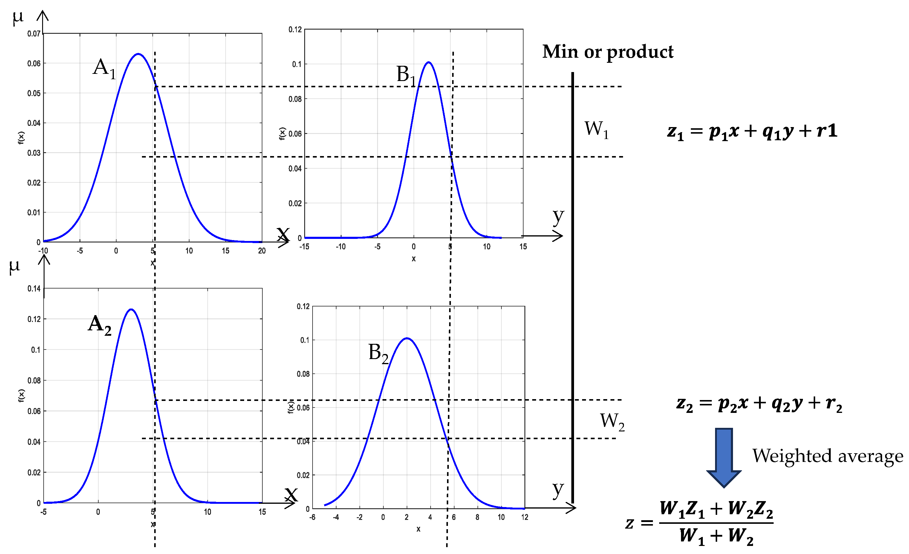
Another type of fuzzy model was proposed by Takagi–Sugeno [20]. The Takagi–Sugeno model is associated with rules based on a specific format. Rather than relying on Mamdani’s vague consequences, this approach is distinguished by functional consequences. The Sugeno model, which has “m” inputs, can be represented as a set of “n” rules following the following structure [36]:

$$R_i:If x_1=A_1^i AND x_2=A_2^i,\dots .AND x_m=A_m^{i}THEN Y_i=a_{i0}+a_{i1}{x}_i+\dots +a_{im}{x}_m$$

The regression parameters represented by ${\mathrm{a}}_{\mathrm{i}0},{\mathrm{a}}_{\mathrm{i}1}{\mathrm{x}}_{\mathrm{i}},\dots ,{\mathrm{a}}_{\mathrm{i}\mathrm{m}}{\mathrm{x}}_{\mathrm{m}}$, where i = 1, 2, 3…n, are adjusted by least squares estimation (LSE).

As shown in Figure 3, the final result is determined by calculating the weighted average of the outputs of each rule, thus producing a linear combination of the input variables added to a fixed term [37].

3. Theoretical Study

3.1. Acoustic Backscattering

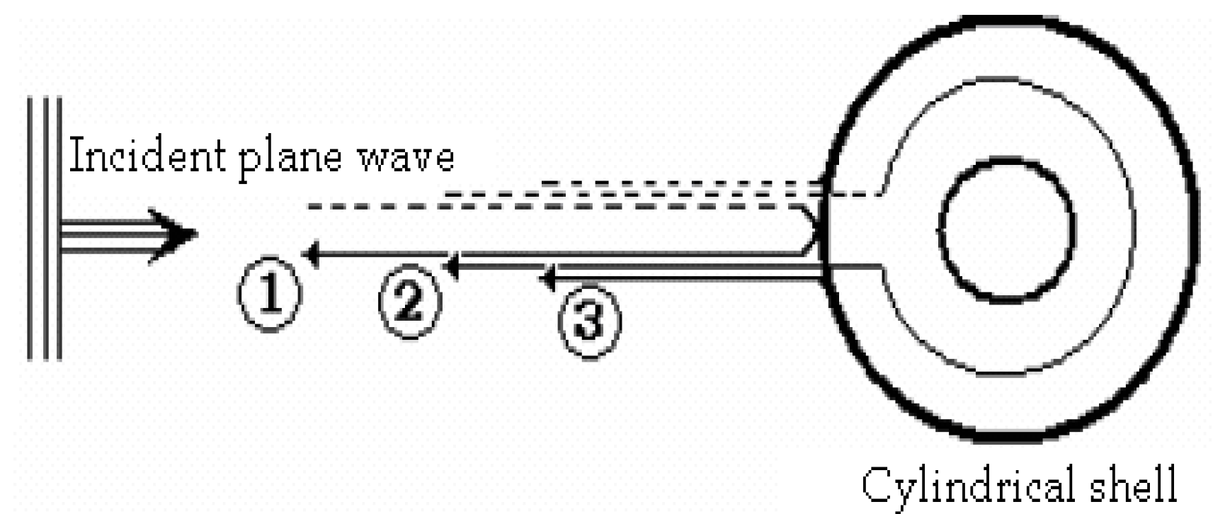
The dispersion of a plane wave by an air-filled cylindrical shell underwater (C₁, velocity of acoustic waves in water) of various radius ratios is investigated by solving the wave equation and the associated boundary conditions [4,5,6,7]. Figure 4 shows the placement of cylindrical coordinates and the direction of a plane wave exciting an infinitely long cylindrical shell in a fluid medium. The density of water is ρ₁, and the acoustic propagation velocity is C₁. Typically, air is characterized by the values C₃ and ρ₃. The parameters for the two fluids, both external and internal to the shell, are presented in

Table 1. Physical parameters.

	Copper	Water (Fluid 1)	Air (Fluid 2)
Density ρ (kg/m3)	8930	1000	1.29
CL: Longitudinal velocity (m/s)	4760	1470	334
CT: Transverse Velocity (m/s)	2325	-----------------	----------------

.

In the system of cylindrical coordinates (r, θ, z), the cylindrical shell’s axis is the z-axis. As shown in Figure 4, we consider a plane wave incident on an infinite cylindrical shell immersed in water (fluid 1) that has an air-filled cavity (fluid 2).

The sum of the incident wave, reflection wave (1), surface wave shell waves (2), symmetric waves $S_{i=0,1,2\dots }$, antisymmetric waves $A_{i=0,1,2\dots }$, and Scholte interface waves (A) (3) is the complex pressure P_diff scattered by a cylindrical shell in the far field (r >> a).

Contributions (2) and (3) correspond to circumferential waves whose properties are directly related to the geometry of the cylindrical shell (see Figure 5).

The form function is a component of the normalized complex backscattered pressure in the far field. This relationship can be utilized to calculate the following function [4,5,38]:

$$\left|P_{scat}\left(\omega \right)\right|={\displaystyle \frac{2}{\sqrt{\pi k_{1}r}}}\left|{\sum }_{n=0}^{N_{max}}{\chi }_n{(-1)}^n{\displaystyle \frac{D_n^1\left(\omega \right)}{D_n\left(\omega \right)}}\right|$$

(6)

where ${\chi }_{\mathrm{n}}$ is the Neumann factor (${\chi }_{\mathrm{n}}=1$, when n = 0; ${\chi }_{\mathrm{n}}=2$, when n > 0), $\mathsf{\omega }=2\mathsf{\pi }\mathrm{f}$ is angular frequency, and ${\mathrm{k}={\displaystyle \frac{\mathsf{\omega }}{\mathrm{C}}}}_1$ is the wave number related to wave velocity in water.

The determinants ${\mathrm{D}}_{\mathrm{n}}^1\left(\mathsf{\omega }\right)$ and ${\mathrm{D}}_{\mathrm{n}}\left(\mathsf{\omega }\right)$ are computed with the boundary conditions (continuity of displacement and stress at both interfaces) taken into consideration.

Table 1 displays the physical parameters that were utilized to determine the backscattered complex pressure.

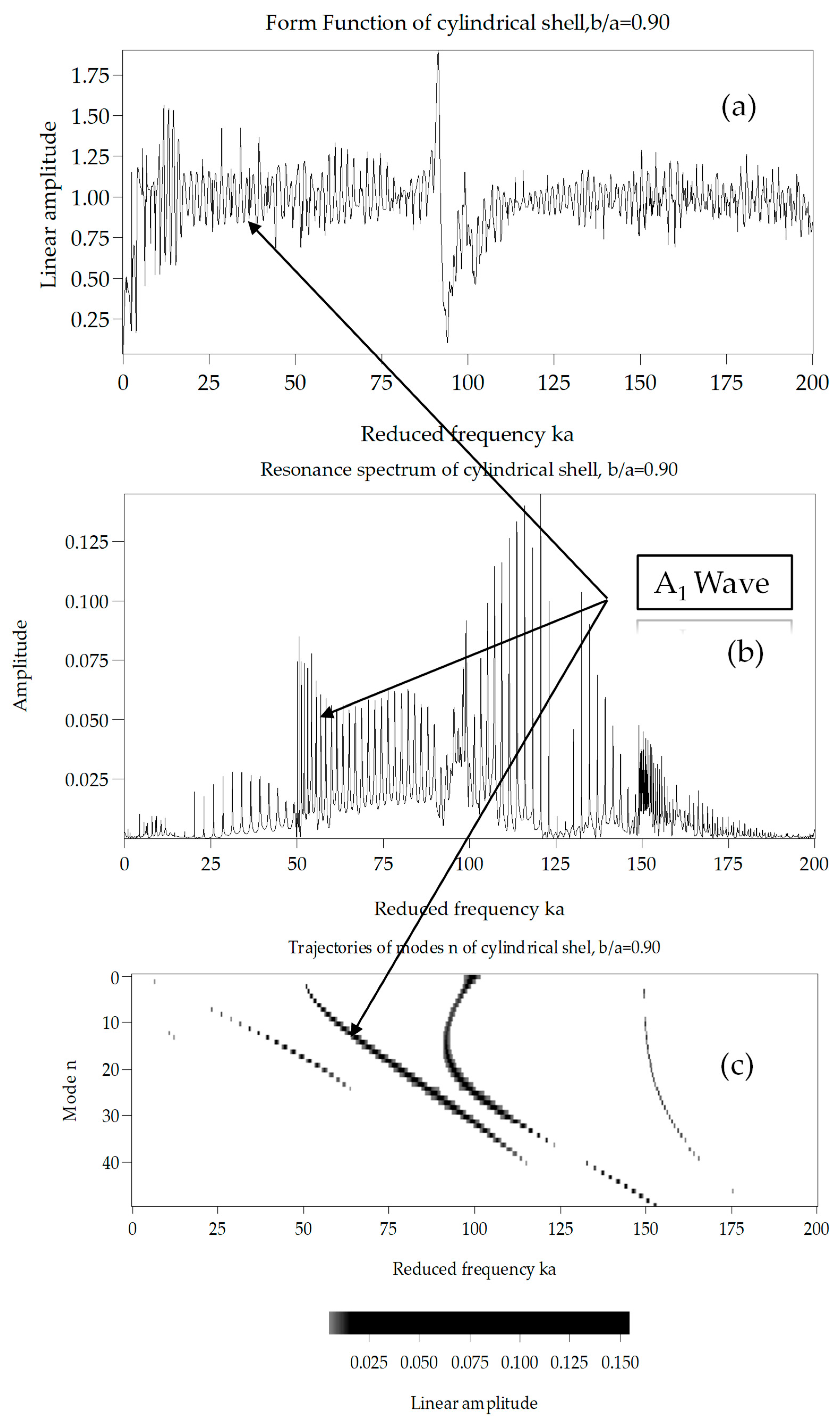
The normalized backscattered complex pressure module is shown against the reduced frequency ka (without the unit) in Figure 6. This is determined by the following:

$$ka={\displaystyle \frac{\omega a}{c}}={\displaystyle \frac{2\pi }{c(1 - \frac{b}{a})}}fd$$

(7)

d = a − b is the cylindrical shell thickness, and f is the incident wave frequency in Hz.

Sharp shell transitions (corresponding to resonance frequencies) in the spectrum of Figure 6a are associated with acoustic wave propagation: the shell has a higher frequency than the resonance frequencies: Scholte waves (A) and shell waves (S₀, A₁, S₁, S₂, A₂…).

3.2. Determination of Phase and Group Velocities

To calculate the phase velocity of the circumferential wave, the resonance spectrum is calculated for each mode n, as shown in Figure 6b. After measuring the resonance frequencies, the phase velocity is given by the following equation:

$$C_{ph}=C_{water}{\displaystyle \frac{x^{\prime }}{n}}=2\pi aF$$

(8)

where x′ = ka is the reduced frequency of the resonance, a represents the outer radius, and F (Hz) is the frequency of the resonance.

Equation (9) is used for the determination of the group velocity:

$$C_{gr}=C_{water}\left(x_{n+1}^{\prime }-x_n^{\prime }\right)=2\pi a(F_{n+1}-F_n)$$

(9)

The variables ${\mathrm{x}}_{\mathrm{n}}^{\prime }$ and ${\mathrm{x}}_{\mathrm{n}+1}^{\prime }$ represent, respectively, the reduced frequencies of the resonances n and n + 1. The variables ${\mathrm{F}}_{\mathrm{n}+1}$ and ${\mathrm{F}}_{\mathrm{n}}$ denote, respectively, the absolute frequencies of the resonances n and n + 1.

4. Methodology

To build a fuzzy model, one must have separate training and test datasets. Fuzzy systems model parameterized nonlinear relationships and, with least-squares estimation, can approximate any regression function [39]. The setup procedure for the process under consideration is:

• Choosing the most crucial elements to include in the modeling procedure.
• Creating a dataset, adapted to the chosen criteria, necessary for training and validation.
• Building the fuzzy model, which is a process that involves using a system identification technique based on subtractive clustering linked to a Sugeno fuzzy inference system.
• Modifying the clustering settings to obtain a model with the least amount of error.

The development of the fuzzy system necessitates identifying the pertinent variables that significantly impact the desired model. This study involves the compilation of a database to assess and evaluate the model’s performance based on the results obtained from the theoretical technique of natural mode trajectories, as shown in Figure 6c.

The material density, radius ratio b/a, antisymmetric wave index i, and propagation velocities within the tube are maintained as pertinent characteristics of the model, as these factors define the tube and the nature of the circumferential waves that propagate around it.

The phase and group velocities of the antisymmetric waves $A_{i=0,1,2\dots }$ are the model’s output. The gathered data used for the fuzzy model’s training and validation stages is shown in

Table 2. Training dataset.

N°	Frequency	Group Velocity Desired (×103)	Group Velocity Predicted (×103)
1	11.7306	0.5996	0.5996
2	12.2698	1.2207	1.2207
3	12.5394	1.4722	1.4722
4	13.0786	1.8772	1.8771
5	13.3482	2.0378	2.0380
6	13.8874	2.2909	2.2905
7	14.1570	2.3887	2.3891
8	14.6961	2.5387	2.5382
9	14.9657	2.5948	2.5952
10	15.5049	2.6779	2.6780
11	15.7745	2.7078	2.7075
12	16.3137	2.7500	2.7506
13	16.5833	2.7643	2.7637
14	17.1225	2.7832	2.7828
15	17.3921	2.7891	2.7900
16	17.9313	2.7960	2.7955
17	18.7401	2.7990	2.7991
18	19.5489	2.7972	2.7981
19	20.3576	2.7919	2.7897
20	21.1664	2.7819	2.7846
21	21.4360	2.7771	2.7791
22	21.9752	2.7647	2.7629
23	22.2448	2.7568	2.7536
24	23.0536	2.7258	2.7255
25	23.5928	2.6980	2.7020
26	24.4016	2.6447	2.6426
27	24.6712	2.6237	2.6214
28	25.2103	2.5771	2.5774
29	25.4799	2.5515	2.5534
30	26.0191	2.4961	2.4973
31	26.2887	2.4664	2.4655
32	26.8279	2.4038	2.4024
33	27.0975	2.3711	2.3716
34	27.6367	2.3035	2.3051
35	27.9063	2.2689	2.2691
36	28.4455	2.1991	2.1972
37	28.7151	2.1642	2.1633
38	29.2543	2.0954	2.0974
39	29.5239	2.0618	2.0633
40	30.0631	1.9971	1.9950
41	30.3327	1.9664	1.9641
42	30.8718	1.9088	1.9106
43	31.1414	1.8824	1.8853
44	31.6806	1.8346	1.8332
45	31.9502	1.8134	1.8101
46	32.4894	1.7772	1.7760
47	32.7590	1.7621	1.7634
48	33.2982	1.7382	1.7420
49	33.5678	1.7293	1.7320
50	34.1070	1.7174	1.7132
51	34.9158	1.7128	1.7104
52	35.1854	1.7142	1.7158
53	35.7246	1.7202	1.7225
54	35.9941	1.7243	1.7251
55	36.5333	1.7334	1.7318
56	36.8029	1.7377	1.7361
57	37.3421	1.7442	1.7445
58	37.6117	1.7456	1.7466
59	38.1509	1.7428	1.7428
60	38.4205	1.7379	1.7375

and

Table 3. Tchicking dataset.

Title 1	Frequency	Group Velocity Desired (×103)	Group Velocity Predicted (×103)
1	12.0002	0.9313	0.9071
2	14.4266	2.4706	2.4705
3	15.2353	2.6407	2.6415
4	16.0441	2.7314	2.7319
5	17.6617	2.7932	2.7942
6	18.4705	2.7987	2.7969
7	19.2793	2.7982	2.8003
8	20.0880	2.7941	2.7918
9	22.5144	2.7478	2.7441
10	23.3232	2.7127	2.7153
11	24.1320	2.6640	2.6638
12	26.5583	2.4356	2.4334
13	27.3671	2.3376	2.3395
14	28.1759	2.2341	2.2327
15	30.6023	1.9369	1.9363
16	31.4110	1.8576	1.8592
17	32.2198	1.7943	1.7911
18	34.6462	1.7128	1.7057
19	36.2637	1.7288	1.7281
20	37.8813	1.7453	1.7460

.

The output model, specifically the phase and group velocities of circumferential antisymmetric modes, is determined by utilizing the aforementioned input factors. The model was constructed using MATLAB R2022b (version 9.13) fuzzy logic toolbox. In both the input and output domains, subtractive clustering was used to develop the model. Each cluster defines specific aspect parts of the system’s behavior. Each input space dimension was filled with the clusters, with each projection delineating an antecedent of a rule. Consequently, the model’s premise parameters were found.

The input variables and the output variable of the identified first-order Sugeno fuzzy model, as described by Jang [35], were the regression parameters determined through the application of the LSE algorithm as outlined by [39]. For a given collection of clusters, the LSE method ensures that the regression parameters are globally optimized. The main goal of system modeling optimization is to determine the ideal range of clustering parameters. These parameters are the squash factor (g), cluster radius (r_a), acceptance ratio ($\overline{\epsilon }$), and reject ratio ($\underset{\_}{\epsilon }$); see

Table 4. Errors for the prediction of group velocity with different fuzzy inference system (FIS) configurations.

Radius ra	Squash Factor ρ	Accept Ratio $(\overline{\mathit{\epsilon }}$)	Reject Ratio $(\underset{\_}{\mathit{\epsilon }}$)	Number of Rules	MAE
0.5	0.4	0.2	0.1	7	0.0900
0.5	0.4	0.2	0.1	8	0.0130
0.5	0.3	0.2	0.1	11	0.0003
0.4	0.3	0.2	0.1	16	0.00028
0.3	0.3	0.2	0.1	19	0.00027
0.5	0.3	0.2	0.1	24	0.0002
0.5	0.3	0.2	0.1	25	0.00015

.

The FIS was trained using one of the two approaches listed below:

• A hybrid optimization technique wherein functional signals progress and consequent parameters are determined using least squares estimation (LSE).
• The backpropagation optimization approach, which propagates error rates backward, updating the parameters based on the gradient descent technique.

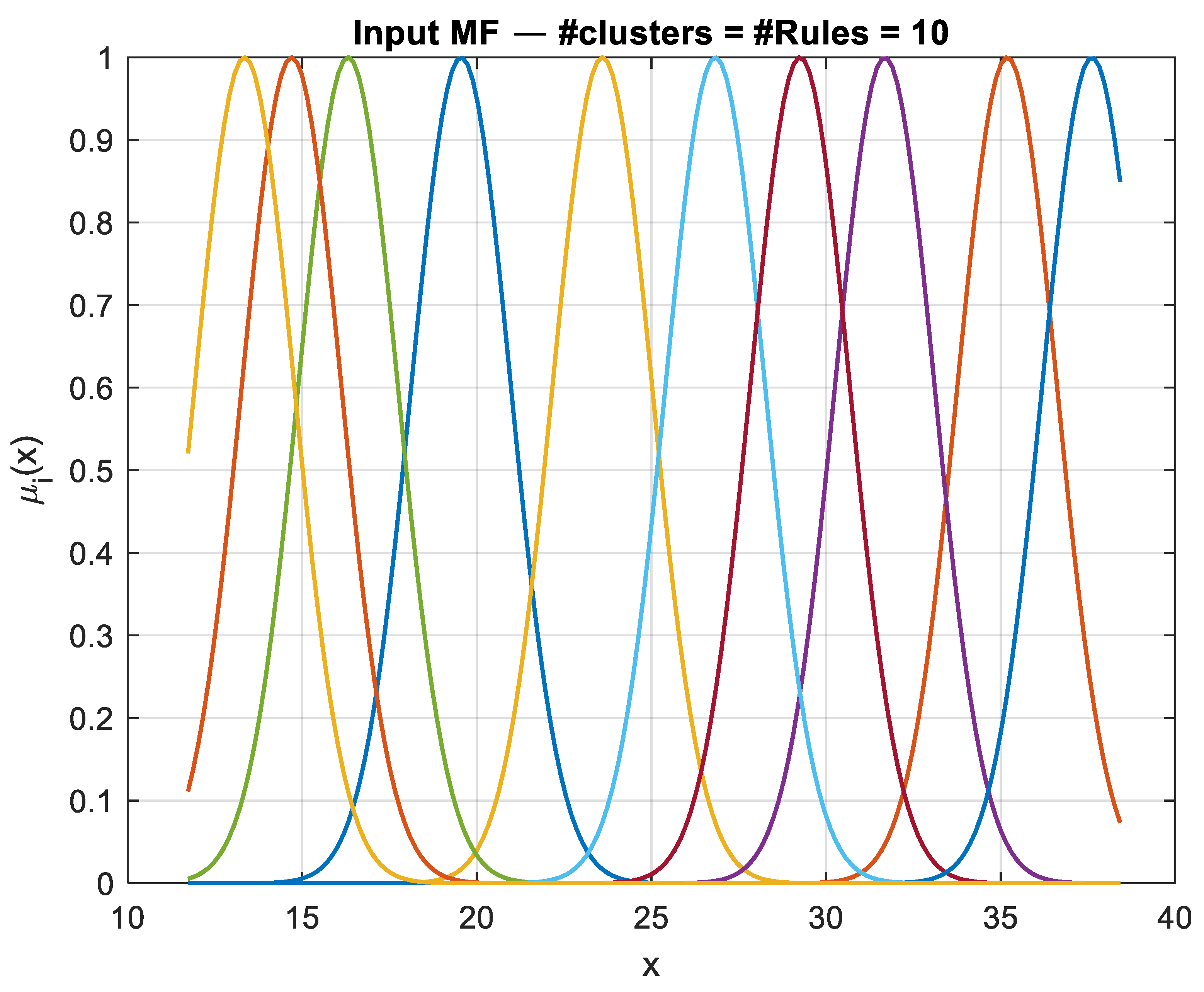
Table 2 and Table 3 report the group velocities of the A₁ circumferential wave for several reduced frequency values in a cylindrical shell with radius ratio b/a = 0.9. Table 2 contains the training subset (two-thirds of the full dataset) used during model learning; this subset is employed to update the shapes of the membership functions (see Figure 7). Table 3 contains the test subset (the remaining one-third), provided only with input variables. For these cases, the trained model must predict the corresponding output (group velocity) within an acceptable error.

This method enables the prediction of group velocity and phase velocity for all antisymmetric circumferential waves A_i and symmetric circumferential waves S_i propagating around a cylindrical shell, for various b/a radius ratios ranging from 0.4 to 0.99, and for different constituent materials such as copper, aluminum, and others.

5. Results and Discussion

The model selection process involves a comparative analysis of error metrics, specifically the MAE, MRE, and SE, to evaluate the discrepancies between the velocities predicted by the fuzzy inference system model and the target velocities. The determination coefficient (R²) and correlation coefficient (R) are used in linear regression analysis to evaluate how well the model performs in respect to the actual desired values and the projected values. The following is a description of the correlation coefficient and the relationships for the various error metrics:

$$MAE={\displaystyle \frac{1}{n}}{\sum }_{i = 1}^n|D_i-P_i|$$

(10)

$$MAE={\displaystyle \frac{1}{n}}{\sum }_{i=1}^n{\displaystyle \frac{|D_i-P_i|}{D_i}}$$

(11)

$$R=1-{\displaystyle \frac{{\sum }_i^n{(D_{i }-{ P}_i)}^2}{{\sum }_i^n{(D_i-{ P}_m)}^2}}$$

(12)

$$SE={\displaystyle \frac{\sqrt{{\sum }_i^n{(D_i-P_i)}^2}}{n-1}}$$

(13)

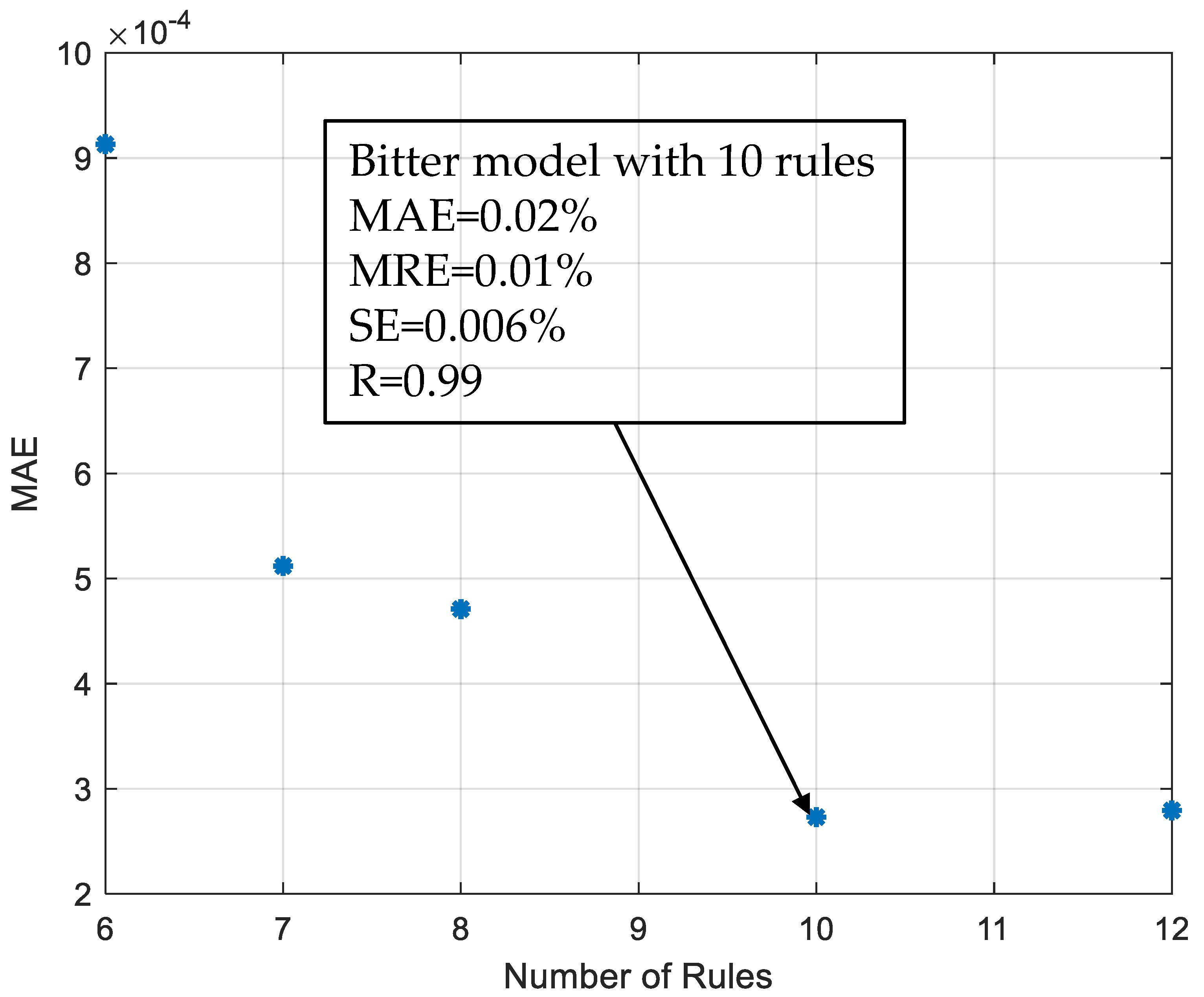
where n is the number of data points; the predicted and desired phase and group velocities are represented by P_i and D_i, respectively; and P_m signifies the mean of the predicted values. The degree and direction of the linear relationship between estimated and observed values are evaluated statistically using the correlation coefficient. Figure 8, Figure 9 and Figure 10 illustrate the performance metrics of the FIS models as applied to both the training and test datasets. The analysis is conducted repeatedly. The error values of each FIS architecture are given by the type of MF and the number of rules; see Figure 7 and Figure 8 and Table 4.

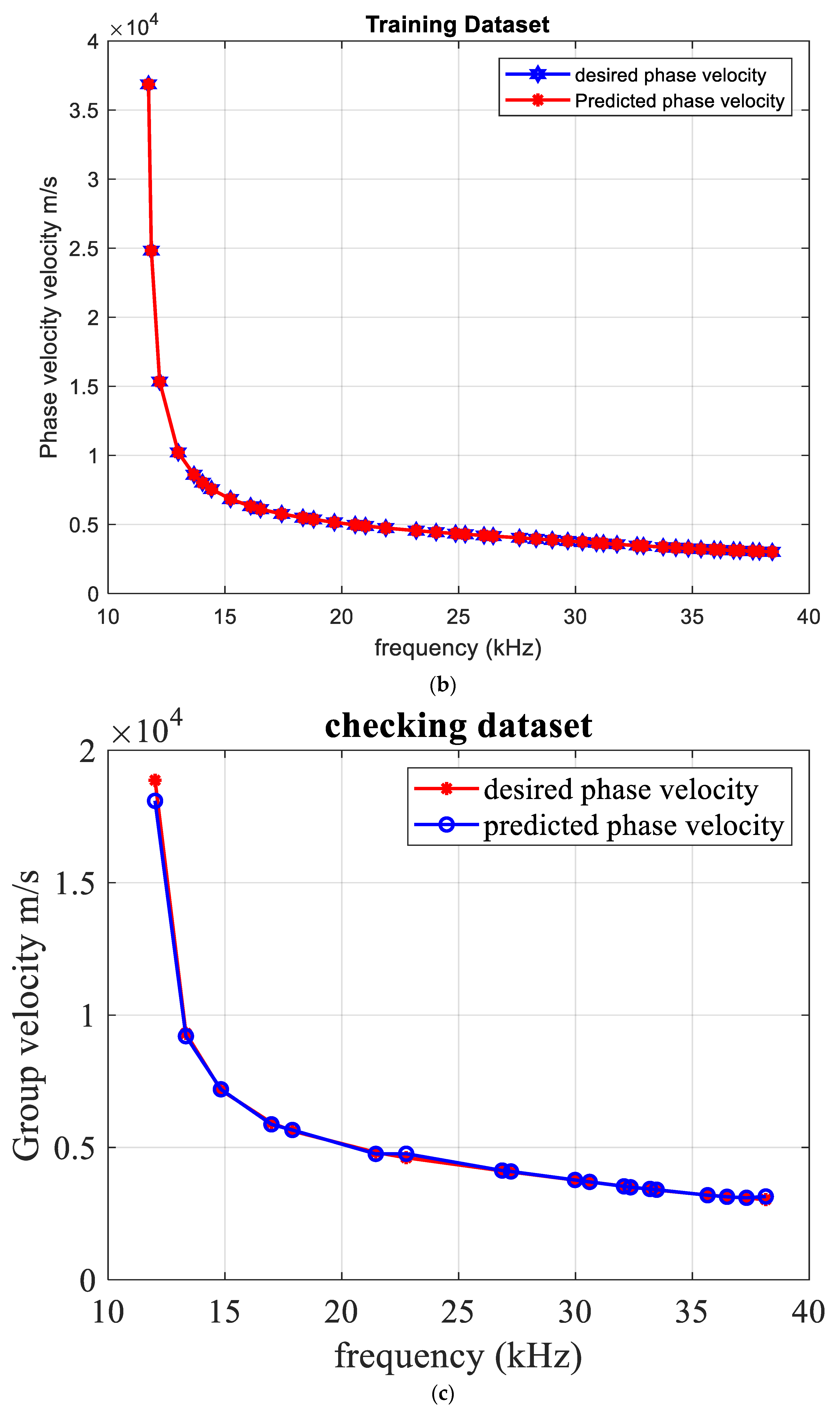
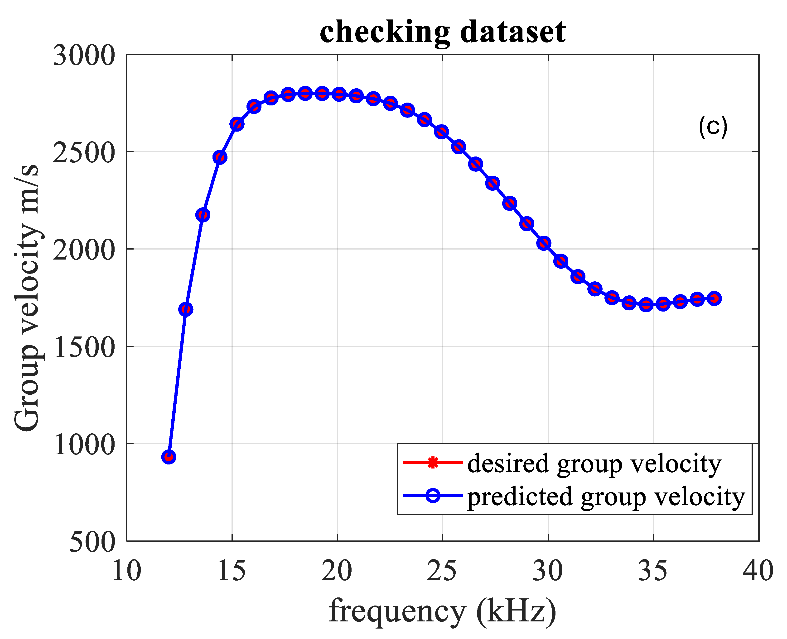
The errors documented for the A₁ circumferential wave are depicted in Figure 9a and Figure 10b. In this investigation, we investigated the number of clusters and discovered that the error of our model values decreased more considerably as the number of clusters increased. The correlation coefficient and error values (MRE, MAE, SE, and R) are summarized in Table 4 and Figure 9a and Figure 10a. Therefore, the fuzzy logic approach is advantageous. The optimal configuration is identified in a model with 11 clusters. A plot of desired versus predicted values is shown in Figure 9 and Figure 10. The results indicate a good correlation between the desired and predicted values of phase and group velocity. The coefficient of determination (R²) is 0.998 for this optimal configuration. Figure 9 demonstrates that the phase velocity decreases as the frequencies take higher values, and this can be justified by the fact that, as the reduced frequency increases, the circumferential wavelength decreases, flexural effects become dominant, the effective stiffness decreases, and the phase velocity drops due to geometric dispersion and the curvature effect. Meanwhile, the group velocity, as shown in Figure 10, increases with frequency up to a maximum point and then decreases from the frequency value around 20 kHz, and this can be justified by the fact that, at very low reduced frequencies, the wave is close to the mode’s cut-off frequency, resulting in a low group velocity because the wave carries little energy along the shell.

As the reduced frequency increases slightly, the circumferential wavelength decreases, and the wave propagates more efficiently, causing the group velocity to rise rapidly. At an intermediate reduced frequency, propagation is dominated by membrane deformations, where the effective stiffness is at its maximum, and the group velocity is high. This is the point at which the group velocity reaches its peak. Beyond this frequency, flexural effects become dominant. The effective stiffness decreases, and geometric dispersion due to curvature slows down the propagation, leading to a decrease in group velocity. At very high reduced frequencies, the mode approaches an asymptotic regime in which dispersion effects are balanced, resulting in a constant group velocity.

In subsequent research, we will utilize time–frequency techniques, like Choi–Williams, Capon, and AOK, in several domains, including biological signal processing; these methods have demonstrated excellent results [40,41,42].

6. Conclusions

In order to forecast the phase and group velocities of circumferential signals in different materials, a model was developed that incorporates specific tube characteristics. In this article, this approach is applied to copper. The optimal model consists of thirteen clusters (rules), with each cluster representing a single fuzzy rule. This model provides accurate predictions of both phase and group velocity values.

By exploiting the analysis of circumferential wave velocities, this work also contributes to the diagnosis of cylindrical shells. Circumferential waves are particularly valuable because they are sensitive to the structural and elastic properties of the tube, which makes them powerful indicators for detecting changes or defects. As such, the developed model not only predicts propagation parameters but also provides a solid basis for the non-destructive evaluation and structural health monitoring (SHM) of tubular structures.

The model can additionally be used to forecast the cut-off dimensionless frequency as a function of the radius ratio and to estimate several tube parameters from known properties. Unlike the natural mode method—which approximates tubes as plates of identical thickness and introduces inaccuracies—the proposed approach avoids such approximations and is not affected by the errors commonly observed in temporal analysis.

To confirm the results, the Wigner–Ville time–frequency distribution applied to the inverse Fourier transform of the shape function provides a representation where circumferential waves, and, in particular, the antisymmetric A1 mode, are clearly identifiable. A drawback of this technique is that it still relies on manual velocity estimation, which makes the procedure somewhat subjective.

In contrast, the proposed model serves as a novel and reliable tool for the characterization and diagnosis of elastic cylindrical shells, enabling the automatic and precise determination of the phase and group velocities of antisymmetric waves propagating around the tube, with direct applications in non-destructive testing, defect detection, and long-term monitoring of tubular structures.

7. Perspectives

The acoustic analysis of cylindrical structures for early defect detection remains challenging due to signal complexity and noise. Subtractive clustering offers a powerful unsupervised method to automatically identify key patterns in acoustic data without prior labeling. By extracting representative clusters, it enables effective signal segmentation and dimensionality reduction.

Combined with fuzzy inference systems, this approach provides flexible and interpretable classification adaptable to varying conditions. Its application holds strong potential for real-time, robust defect detection and predictive maintenance in industrial structures.

References

1. Yin, T.; Ng, C.T.; Vidler, J.; Ho, V.D.; Kotousov, A. Amplitude-modulation vibro-acoustic technique for damage evaluation, Construction and Building Materials. Struct. Heal. Monit. 2022, 346, 128381. [Google Scholar]
2. Hu, X.; Ng, C.T.; Kotousov, A. Numerical and experimental investigations on mode conversion of guided waves in partially immersed plates. Measurement 2022, 190, 110750. [Google Scholar] [CrossRef]
3. Nahraoui, Y.; Aassif, E.H.; Maze, G. Modeling of the thickness of a Submerged Tube by the Artificial Neural Network. In Proceedings of the International Conference on Multimedia Computing and Systems, Mountain View, CA, USA, 27–31 October 2017; pp. 583–587. [Google Scholar]
4. Flax, L.; Dragonette, L.; Uberall, H. Theory of elastic resonance excitation by sound scattering. J. Acoust. Soc. Amer. 1978, 63, 723–731. [Google Scholar] [CrossRef]
5. Maze, G. Acoustic scattering from submerged cylinders. MIIR Im/Re: Experimental and theoretical study. J. Acoust. Soc. Amer. 1991, 89, 2559–2566. [Google Scholar] [CrossRef]
6. Haumesser, L.; Décultot, D.; Léon, F.; Maze, G. Experimental identification of finite cylindrical shell vibration modes. J. Acoust. Soc. Am. 2002, 111, 2034–2039. [Google Scholar] [CrossRef] [PubMed]
7. Maze, G. Diffusion D’une Onde Acoustique Plane Par des Cylindres et Tubes Immergés Dans L’eau: Isolement et Identification des Résonances, Thèse de Doctorat d’Etat és-Sciences; University of Rouen: Rouen, France, 1984. (In French) [Google Scholar]
8. Maze, G.; Izbicki, J.L.; Ripoche, J. Resonances of plates and cylinders: Guided waves. J. Acoust. Soc. Amer. 1985, 77, 1352–1357. [Google Scholar] [CrossRef]
9. Nahraoui, Y.; Aassif, E.; Elhanaoui, A.; Maze, G. A Neuro-Fuzzy Computing Technique for Modeling the Acoustic Form Function of Immersed Tubes. In Proceedings of the 3rd International Conference on Information Systems and Technologies, Tangier, Morocco, 22–24 March 2013. [Google Scholar]
10. Dariouchy, A.; Aassif, E.H.; Decultot, D.; Maze, G. Acoustic characterization and prediction of the cut-off dimensionless frequency of an elastic tube by neural networks. IEEE Trans. Ultrason. Ferroelectr. Freq. Control. 2007, 54, 1055–1064. [Google Scholar] [CrossRef]
11. Tan, L.; Fan, J.; Wang, B.; Zhao, K.; Li, B. Backscattering enhancements by partially exposed cylindrical shells due to reflected flexural waves at air–water interfaces. J. Ocean Eng. Sci. 2023, 10, 274–280. [Google Scholar] [CrossRef]
12. Thinh, T.I.; Nguyen, M.C. Dynamic stiffness method for free vibration of composite cylindrical shells containing fluid. Appl. Math. Model. 2016, 40, 9286–9301. [Google Scholar] [CrossRef]
13. Latif, R.; Aassif, E.; Maze, G.; Moudden, A.; Faiz, B. Determination of the group and phase velocities from time-frequency representation of Wigner-Ville. J. Non-Destr. Test. Eval. Int. 1999, 32, 415–422. [Google Scholar] [CrossRef]
14. Maze, G.; Léon, F.; Ripoche, J.; Überall, H. Repulsion phenomena in the phase-velocity dispersion curves of circumferential waves on elastic cylindrical shells. J. Acoust. Soc. Am. 1999, 105, 1695–1701. [Google Scholar] [CrossRef]
15. Werro, N. Fuzzy Classification of Online Customers; Springer: Heidelberg, Germany, 2015; Volume 148, pp. 1–200. [Google Scholar]
16. Wee, C.T. Advances in Fuzzy Rule-Based System for Pattern Classification. Ph.D. Thesis, National University of Singapore, Singapore, 2010. [Google Scholar]
17. Babuška, R.; Babuška, R. Fuzzy Modeling for Control, 1st ed.; Springer: Dordrecht, The Netherlands, 1998; pp. 13–260. [Google Scholar]
18. Zadeh, L. Outline of a new approach to the analysis of complex systems and decision processes. IEEE Trans. Syst. Man Cybern. 1973, SMC-3, 28–44. [Google Scholar]
19. Mamdani, E. Application of fuzzy logic to approximate reasoning using linguistic systems. Fuzzy Sets Syst. 1977, 26, 1182–1191. [Google Scholar]
20. Takagi, T.; Sugeno, M. Fuzzy identification of systems and its application to modeling and control. IEEE Trans. Syst. Man Cybern. 1985, 15, 116–132. [Google Scholar]
21. Dubois, D.; Prade, H. Fuzzy Sets and Systems—Theory and Applications; Academic Press: New York, NY, USA, 1980; pp. 1–400. [Google Scholar]
22. Bouchon-Meunier, B. La logique floue et ses Applications; Addison-Wesley: Paris, France, 1995; pp. 1–320. [Google Scholar]
23. Yager, R.R.; Filev, D.P. Essentials of Fuzzy Modeling and Control; John Wiley & Sons: New York, NY, USA, 1994; pp. 1–320. [Google Scholar]
24. Zadeh, L. Fuzzy sets. Inf. Control. 1965, 8, 338–353. [Google Scholar] [CrossRef]
25. Driankov, D.; Hellendoorn, H.; Reinfrank, M. An Introduction to Fuzzy Control; Springer: Berlin, Germany, 1993; pp. 1–304. [Google Scholar]
26. Galichet, S. Contrôle Flou de L’interpolation Numérique au Codage de L’expertise. In Habilitation à Diriger des Recherches; Université de Savoie: Annecy, France, 2001. [Google Scholar]
27. Singh, S.; Rattan, K.S. Implementation of a fuzzy logic controller on an FPGA using VHDL. In NAFIPS 2003 22nd International Conference of the North American; Fuzzy Information Processing Society: West Lafayette, IN, USA, 2003; pp. 110–115. [Google Scholar]
28. Vuong, P.T.; Madni, A.M.; Vuong, B. VHDL Implementation for a Fuzzy Logic Controller. In Automation Congress; WAC ’06 World: Budapest, Hungary, 2006; pp. 1–8. [Google Scholar]
29. Abu-Khudhair, A.; Muresan, R.; Yang, S.X. FPGA Based Real-Time Adaptive Fuzzy Logic Controller. In Proceedings of the 2010 IEEE International Conference on Automation and Logistics (ICAL), Beijing, China, 16–20 August 2010; pp. 539–544. [Google Scholar]
30. Borne, P.; Rozinoer, I.; Dieulot, I.-Y.; Dubois, L. Introduction à la Commande Floue; Technip: Paris, France, 1998; pp. 1–320. [Google Scholar]
31. Passino, K.M.; Yurkovich, S.; Reinfrank, M. Fuzzy Control; Addison-Wesley: Boston, MA, USA, 1998; Volume 42, pp. 15–21. [Google Scholar]
32. Oliveira, D.N.; de Lima Henn, G.A.; da Mota Almeida, O. Design and implementation of a Mamdani Fuzzy Inference System on an FPGA using VHDL. In Proceedings of the Fuzzy Information Processing Society (NAFIPS), 2010 Annual Meeting of the North American, Toronto, ON, Canada, 12–14 July 2010; pp. 1–6. [Google Scholar]
33. Chiu, S. Fuzzy model identification based on cluster estimation. J. Intell. Fuzzy Syst. 1994, 2, 267–278. [Google Scholar] [CrossRef]
34. Demirli, K.; Muthukumaran, P. Higher order fuzzy system identification using subtractive clustering. J. Intell. Fuzzy Syst. 2000, 9, 129–158. [Google Scholar] [CrossRef]
35. Jang, J.-S.R.; Sun, C.-T.; Mizutani, E. Neuro-Fuzzy and Soft Computing: A Computational Approach to Learning and Machine Intelligence; Prentice-Hall: Englewood Cliffs, NJ, USA, 1997; pp. 1–614. [Google Scholar]
36. Mamdani, E.; Assilian, S. An Experiment in Linguistic Synthesis Using a Fuzzy Logic Controller. Int. J. Man-Mach. Stud. 1975, 7, 1–13. [Google Scholar] [CrossRef]
37. Hayajneh, M.T.; Hassan, A.M.; Al-Wedyan, F. Monitoring Defects of Ceramic Tiles Using Fuzzy Subtractive Clustering-Based System Identification Method. Soft Comput. 2010, 14, 615–626. [Google Scholar] [CrossRef]
38. Maze, G.; Ripoche, J.; Derem, A.; Rousselot, J.L. Diffusion d’une onde ultrasonore par des tubes remplis d’air immergés dans l’eau. Acustica 1984, 55, 69–85. [Google Scholar]
39. Jang, J. ANFIS: Adaptive-Network-Based Fuzzy Inference System. IEEE Trans. Syst. Man Cybern. 1993, 23, 665–685. [Google Scholar]
40. Elouaham, S.; Nassiri, B.; Dliou, A.; Zougagh, H.; El Kamoun, N.; El Khadiri, K.; Said, S. Combination Time-Frequency and Empirical Wavelet Transform Methods for Removal of Composite Noise in EMG Signals. Telkomnika Telecommun. Comput. Electron. Control 2023, 21, 1373–1381. [Google Scholar] [CrossRef]
41. El Khadiri, K.; Elouaham, S.; Nassiri, B.; El Melhoaui, O.; Said, S.; El Kamoun, N.; Zougagh, H. A Comparison of the Denoising Performance Using Capon Time-Frequency and Empirical Wavelet Transform Applied on Biomedical Signal. Int. J. Eng. Appl. (IREA) 2023, 11, 358–365. [Google Scholar] [CrossRef]
42. Elouaham, S.; Dliou, A.; Laaboubi, M.; Latif, R.; Elkamoun, N.; Zougagh, H. Filtering and analyzing normal and abnormal electromyogram signals, Indonesia. J. Electr. Eng. Comput. Sci. 2020, 20, 176–184. [Google Scholar]
Figure 1. Typical shapes representing membership functions.
Signals 06 00056 g001
Figure 2. The fuzzy inference system’s structure.
Signals 06 00056 g002
Figure 3. The Sugeno fuzzy model [35].
Signals 06 00056 g003
Figure 4. Geometry of cylindrical shell [10].
Signals 06 00056 g004
Figure 5. Process of generating echoes: (1) specular reflection; (2) circumferential waves in shells; and (3) Scholte wave (A) [10].
Signals 06 00056 g005
Figure 6. The wave localization of circumferential waves as a function of frequency. (a) Backscattered pressure. (b) A resonance spectrum. (c) Mode n trajectories for a cylindrical copper shell (b/a = 0.90). The link between transition (a) and peak (b) is shown by vertical arrows. A vertical line indicates the A1 wave’s cut-off dimensionless frequency.
Signals 06 00056 g006
Figure 7. Gaussian membership function. Each membership function is represented by a colored curve, allowing us to distinguish between the different membership functions. Each membership function corresponds to a fuzzy set, which also defines a fuzzy rule.
Signals 06 00056 g007
Figure 8. Errors for the prediction of group velocity with different fuzzy inference systems. * Represents the Mean Absolute Error (MAE) as a function of the number of rules. Each asterisk corresponds to the MAE value for a specific number of rules.
Signals 06 00056 g008
Figure 9. (a) Correlation between desired and predicted phase velocity. (b) Training dataset (wave A1) showing evolution of group velocity compared to growth of frequency. (c) Validation dataset (wave A1).
Signals 06 00056 g009aSignals 06 00056 g009b
Figure 10. (a) Correlation between desired and predicted group velocity. (b) Training dataset (wave A1) showing evolution of group velocity compared to growth of frequency. (c) Validation dataset (wave A1).
Signals 06 00056 g010aSignals 06 00056 g010b