Article

Intelligent Face Recognition: Comprehensive Feature Extraction Methods for Holistic Face Analysis and Modalities

by
Thoalfeqar G. Jarullah
1,
Ahmad Saeed Mohammad
1,*,
Musab T. S. Al-Kaltakchi
2 and
Jabir Alshehabi Al-Ani
3
1
Department of Computer Engineering, College of Engineering, Mustansiriyah University, Baghdad 10047, Iraq
2
Department of Electrical Engineering, College of Engineering, Mustansiriyah University, Baghdad 10047, Iraq
3
Department of Data Science, York St. John University, York YO31 7EX, UK
*
Author to whom correspondence should be addressed.
Signals 2025, 6(3), 49; https://doi.org/10.3390/signals6030049
Submission received: 15 May 2025 / Revised: 22 July 2025 / Accepted: 4 August 2025 / Published: 19 September 2025

Abstract

Face recognition technology utilizes unique facial features to analyze and compare individuals for identification and verification purposes. This technology is crucial for several reasons, such as improving security and authentication, effectively verifying identities, providing personalized user experiences, and automating various operations, including attendance monitoring, access management, and law enforcement activities. In this paper, comprehensive evaluations are conducted using different face detection and modality segmentation methods, feature extraction methods, and classifiers to improve system performance. As for face detection, four methods are proposed: OpenCV’s Haar Cascade classifier, Dlib’s HOG + SVM frontal face detector, Dlib’s CNN face detector, and Mediapipe’s face detector. Additionally, two types of feature extraction techniques are proposed: hand-crafted features (traditional methods: global local features) and deep learning features. Three global features were extracted, Scale-Invariant Feature Transform (SIFT), Speeded Robust Features (SURF), and Global Image Structure (GIST). Likewise, the following local feature methods are utilized: Local Binary Pattern (LBP), Weber local descriptor (WLD), and Histogram of Oriented Gradients (HOG). On the other hand, the deep learning-based features fall into two categories: convolutional neural networks (CNNs), including VGG16, VGG19, and VGG-Face, and Siamese neural networks (SNNs), which generate face embeddings. For classification, three methods are employed: Support Vector Machine (SVM), a one-class SVM variant, and Multilayer Perceptron (MLP). The system is evaluated on three datasets: in-house, Labelled Faces in the Wild (LFW), and the Pins dataset (sourced from Pinterest) providing comprehensive benchmark comparisons for facial recognition research. The best performance accuracy for the proposed ten-feature extraction methods applied to the in-house database in the context of the facial recognition task achieved 99.8% accuracy by using the VGG16 model combined with the SVM classifier.
Keywords:
SIFT; SURF; GIST; LBP; WLD; HOG; CNN; VGG16; VGG19; VGG-face

1. Introduction

Intelligent Face Recognition (IFR) aims to transform identification processes by harnessing advanced algorithms and machine learning techniques to analyze and compare intricate facial features. This technology plays a critical role in various sectors, including security, authentication, and personalization. By accurately identifying individuals based on unique facial characteristics, IFR enhances user experiences, strengthens security measures, and streamlines processes such as attendance tracking and access management. Moreover, IFR is instrumental in law enforcement, where it aids in identifying suspects and locating missing persons [1,2,3].
Facial recognition is a technology designed to identify and verify individuals based on their facial features. It employs computer algorithms and machine learning techniques to analyze and compare unique facial patterns, including the spacing between the eyes, nose, and mouth, along with other facial characteristics.
Facial recognition systems are employed for a variety of applications, such as user identification, customization, security, and surveillance, in various sectors. These systems capture facial images, process them, and then compare them to historical facial datasets to determine if there is a match which yields the person’s identification.
Different surveys of facial recognition are produced in [4,5,6,7,8]. Furthermore, new research papers are presented as review papers [9,10,11].
The study in [12] examines the possibilities and restrictions of face recognition technology in person identification, particularly with certain demographics and certain traits. As per this study, instances of ethical issues such as false identification and misrepresentation can occur. The study examines the challenges of deploying facial recognition technology, including achieving widespread adoption and verifying distinct identities. The study grounds its framework in the recognition theories of Charles Taylor and Axel Honneth. These types of false identification examines how facial recognition impacts individuals’ self-perception.
Kamil et al. [13] propose a face recognition and facial mask detection-based online attendance recording system. The primary aim of their work is to develop a reliable, web-accessible attendance solution that eliminates the need for dedicated software installation. The system simplifies attendance monitoring by storing records in a centralized online database, accessible via any web-enabled device. The system utilizes individual face-image samples to generate user profiles and establish biometric signatures through facial images. The facial recognition training of the SVM model involves a stage where synthetic data are employed to detect mask-covered facial images. The development of the server application is executed using Python programming language, and image processing is carried out using the Open-Source Computer Vision (OpenCV) module. The database and web interfaces are established using PHP and MySQL. The integration of PHP and Python utilities cloud processing and remote accessibility. Based on the findings and analyses, the results indicate that a pre-trained model achieves high accuracy of approximately 81.8% in recognizing faces and an accuracy of 80% in detecting mask-covered facial images.
Recent years have witnessed growing enthusiasm for facial recognition technology [14], with deep convolutional neural networks (CNNs) demonstrating significant advancements in this field. However, these deep learning models require substantial computational time and large amounts of labeled training data. The research in [14] investigates how transfer learning approaches can optimize both the performance and efficiency of CNN-based facial recognition systems. Specifically, the study evaluates how combining feature extraction with fine-tuning of pre-trained models enables effective knowledge transfer between diverse domains. An enhanced version of the FaceNet model utilizes a MobileNetV2 backbone integrated with a Single Shot MultiBox Detector (SSD) component [15]. The improvements focus on adopting depth-wise separable convolutions to reduce the model’s size and computational requirements while achieving high accuracy and processing speed. The research addresses the challenge of identifying individuals as they move in and out of specified zones, operating within the limitations of modern mobile devices, which include restricted memory capacity and on-device storage constraints. Notably, the proposed approach in [15] demonstrates practical success, achieving over a 95% accuracy on a small dataset of original facial images. Additionally, the resulting frame rate of 25 FPS (Frames Per Second) proves particularly advantageous compared to other neural network-based facial recognition methods.
In the study [16], a novel technique is developed by combining Linear Discriminant Analysis (LDA) with a one-dimensional deep convolutional neural network (1D-DCNN) classifier, forming an innovative face recognition approach. The key contribution involves generating a one-dimensional facial feature set using LDA, derived from the original image dataset. This set is then used to train the 1D-DCNN classifier, improving facial recognition performance. Evaluations are conducted using the MCUT dataset, which contains 3755 images spanning 276 classes. The implementation achieves outstanding results, attaining 100% accuracy, precision, recall, and F-measure.
In this paper, to optimize system performance, comprehensive evaluations are conducted using multiple face recognition techniques and modalities, including segmentation, feature extraction methods, and classifiers. Four face detection approaches are proposed: Mediapipe’s face detector, Dlib’s CNN face detector, Dlib’s HOG + SVM frontal face detector, and OpenCV’s Haar Cascade classifier. Additionally, two distinct feature extraction strategies are introduced: hand-crafted features (traditional methods), categorized into global and local features, and deep learning features (features learned through training algorithms). For global features, three techniques are employed: SIFT, SURF, and GIST.
For local features, three methods are used: WLD, HOG, and LBP. The deep learning features are further subdivided into Siamese neural networks (SNNs), also referred to as face embeddings, and convolutional neural networks (CNNs). Three additional classifiers are proposed: SVM, SVM one-vs-all, and Multilayer Perceptron (MLP). The system is evaluated on three datasets: in-house, LFW, and the Pins dataset. These extensive assessments establish a benchmark for researchers addressing facial recognition challenges. The key contributions of this paper are summarized as follows:
  • Experiment 1: Comprehensive evaluations are conducted on ten feature extraction methods. These methods include SIFT, SURF, and GIST as global features. On the other hand, the other three methods are utilized for local features: LBP, WLD, and HOG. The deep learning (CNN) features are classified into VGG16, VGG19, VGG-face, and SNN, also known as face embeddings. Two classifiers, MLP and SVM, are used for both whole faces and face modalities in the in-house database.
  • Experiment 2: The best result feature extraction method (VGG16), as determined in Experiment 1, is employed to evaluate exclusively whole faces on the LFW and Pins databases, utilizing both MLP and One-vs-All SVM classifiers for assessment.
The paper is structured as follows: The suggested approach is presented in Section 2, the datasets are described in Section 3, the results and discussion appear in Section 4, and the conclusions are presented in Section 5.

2. Proposed Method

The main framework of the proposed method is illustrated in Figure 1. As shown in Figure 1, the proposed system structure is divided into the sections: pre-processing and histogram equalization, face detection and modalities segmentation, further processing on the detected face, feature extraction methods, and classification methods.

2.1. Preprocessing and Histogram Equalization

Contrast-enhancing techniques like Contrast-Limited Adaptive Histogram Equalization (CLAHE) [17] are used during preprocessing by using the following equation:
h ( v ) = r o u n d ( C D F ( v ) m i n ( C D F ) ( W H ) m i n ( C D F ) ) ( L 2 ) ) + 1
where L is the number of gray levels in the image, W is the width of the image, H is the height of the image, and CDF is the Cumulative Distribution Function. Histogram equalization is a method intended to expand an image’s histogram and hence boost contrast. It is frequently used in image processing and is essential for improving the aesthetic appeal of photographs. This equalization yields to the discovery of embedded information and enhances overall image clarity by spreading the pixel values. A proposed technique [18] employed histogram equalization to extract the visual impact of photos used by photographers, graphic designers, and academics through contrast enhancement.

2.2. Face Detection and Modalities Segmentation

Facial detection within captured images is performed through multiple methodologies, each selected based on specific precision and speed requirements. As mentioned previously, these techniques include OpenCV’s Haar Cascade classifier, Dlib’s HOG + SVM frontal face detector, Dlib’s CNN face detector, and Mediapipe’s face detector. Each approach presents unique advantages and computational trade-offs for detecting accuracy and processing efficiency.
OpenCV Haar Cascade classifier is implemented as an object detection technique. This technique scans the entire image with a small window by utilizing a series of straightforward classifiers. In this scenario, the object of interest is the face. The cascade classifier searches for facial characteristics that could potentially be presented in it. The next step is searching for the next feature conditioned by detecting the first feature. The procedure continues until either all cascade classifiers find the designated characteristics or none of them do. As a final result, the detected area under the ROI is confirmed to be the face.
As for the experimental setup, the Python and C++ programming languages were used as these languages are supported by the machine learning and computer vision. The Dlib library, which includes the HOG + SVM frontal face detectors is an additional advantage. It includes an SVM and Histogram of Oriented Gradients (HOG) detector that produces better accuracy compared the Haar Cascade classifier in detecting frontal-view face images (those facing the camera straight without tilting) [19,20].
This approach utilizes the feature extraction technique HOG to extract pertinent characteristics. The main concept is computing the histogram of gradients of a picture. The SVM is also an important part of this approach.
Using this technique, a window slides over the whole picture and HOG features are extracted as the SVM model is then used to identify whether the region contains faces. The detection of faces of varied sizes is facilitated by repeating this technique over many picture pyramids, which represent varying scales for the same image.
Dlib implements an alternative face detection system utilizing convolutional neural networks (CNNs), which operates fundamentally differently from its HOG-based counterpart. CNNs are neural networks capable of extracting features from images without the need for hand-crafted feature selection. The main leverage of the CNN face detector over standard methods is the capability of detecting both tilted and non-frontal faces. However, it comes with expensive power consumption such as using GPU acceleration to achieve real-time performance. This is the result of a higher demand of computational resources compared to the standard or baseline techniques [19,21].
Mediapipe, a computer vision library developed by Google, offers a suite of applications, including a face detection module that employs a distinctive approach distinct from traditional sliding-window methods. This module utilizes an enhanced version of the Single-Shot Multi-Box Detector (SSD), a convolutional neural network (CNN)-based technique, which replaces conventional detection frameworks. The SSD architecture is optimized for efficiency and accuracy, leveraging modern deep learning advancements.
The SSD-based method demonstrates significant advantages, particularly in computational efficiency. It achieves rapid execution on mobile GPUs, delivering high precision while substantially outperforming sliding-window approaches in processing speed reaching frame rates of up to 1000 FPS. These attributes make it particularly suitable for real-time facial recognition on resource-constrained devices. However, a notable limitation is its reliance on close-proximity facial capture to ensure detection accuracy, which may restrict its applicability in scenarios requiring broader field-of-view coverage.
Following face localization, the identification process proceeds with facial modality segmentation, which isolates specific regions such as the eyebrows, eyes, lips, and nose. These modalities can be analyzed individually or in combination to facilitate subject identification. A key advantage of single-modality analysis lies in its potential to accelerate inference speeds, as models trained on isolated features require less computational overhead than whole-face recognition. In this study, modality segmentation is achieved through the application of the following two foundational techniques, balancing precision and efficiency [22,23]: one, the Landmark Detector for Dlib, and two, the Face Mesh Detector from Mediapipe.

2.3. Further Preprocessing

Additional preprocessing is implemented to improve facial recognition performance after facial identification and facial landmarks. Mainly these preprocessing steps are face normalization and alignment.
Face alignment includes adjusting slanted faces using facial landmarks. Face alignment increased the reliability and accuracy of face recognition, according to empirical data. On the other hand, normalization involved changing the image’s pixel values from their original range of 0 to 255 to a range between zero and one. This specific step has been seen to lead to shorter training periods and a minor improvement in training accuracy.

2.4. Feature Extraction Methods

In this study, as shown in Figure 1, hand-crafted features (conventional techniques) are divided into two primary categories—global and local. These features are compared against deep learning features. The features, as explained earlier, are SIFT, SURF, and GIST as the global features, and the local features are WLD, the HOG, and LBP. These contrast with modern deep learning approaches where feature representation emerges automatically through architectures like face embeddings (SNNs) and convolutional neural networks (CNNs).
Following facial localization, the feature extraction process transforms raw image data into compact, discriminative representations. This critical transformation enables effective pattern recognition by subsequent classification algorithms. The current framework implements both traditional and deep learning-based feature extraction methods, with each category containing distinct sub-methods as depicted in Figure 1.
Hand-made features are the foundational kind of feature extraction method. These carefully designed algorithms selectively capture discriminating patterns while suppressing irrelevant image data. The methodology classifies these features into global features, which analyze complete facial images, and local features, which examine specific facial regions. Empirical evidence demonstrates that combining both feature types enhances recognition accuracy [24,25], as they provide complementary visual information at different scales.
This study belongs in the global category. The three global category algorithms are Global Image Structure (GIST), Scale-Invariant Feature Transform (SIFT), and Speeded Up Robust Features (SURF). One of the most significant feature extraction techniques in computer vision is SIFT [26]. It is a scale-, rotation-, illumination-, and viewpoint-invariant feature extraction technique. This technique’s feature extraction process is rather time-consuming.
The following steps are implemented to calculate SIFT features: The scale space is established using Gaussian convolution. Then, the scale space’s Gaussian difference is calculated. Through the difference in Gaussian calculations, key points are discovered while weak key points are rejected. Utilizing the slopes in the immediate vicinity, a reference orientation is given to each significant site to determine the descriptions for every important point.
SURF and SIFT exhibit comparable performance in many respects, including invariance to rotation, scale, lighting, and perspective changes. However, SURF demonstrates significantly faster processing speeds compared to SIFT [27]. This efficiency advantage arises from SURF’s use of integral images and box filters. Instead of repeatedly down-scaling the image and applying Gaussian filters as SIFT does SURF efficiently constructs its scale space by adjusting the box filter size. As a result, SURF achieves processing speeds roughly three times faster than SIFT without sacrificing accuracy.
The GIST (Global Image Structure) descriptor provides a holistic representation of an image. To compute it, the input image is processed using 32 Gabor filters across eight orientations and four scales, generating 32 feature maps matching the original image dimensions. These maps are then divided into a 4 × 4 grid, and the average values of each block are calculated. By concatenating the 16 blocks from every feature map, a compact descriptor is formed, capturing the image’s gradient structure. This method proves effective for tasks like face recognition [28].
Unlike SIFT and SURF, GIST demonstrates superior performance evidenced by the experimental results. Its capability to encode global structural information makes it particularly suitable for applications requiring robust scene or facial representation.
In this study, the local feature extraction techniques include Local Binary Pattern (LBP) [29], Weber Local Descriptor (WLD) [30], and Histogram of Oriented Gradients (HOG) [31]. LBP is one of the most widely used techniques for sentiment analysis and conventional face recognition. For applications like face identification, pedestrian detection, and others, HOG is a well-liked descriptor. Weber is a straightforward and effective local descriptor that is unaffected by variations in lighting, contrast, and geometrical configuration.
The Local Binary Pattern (LBP) operator extracts texture information by comparing each pixel with its neighbors, encoding patterns that are computationally efficient and lighting-invariant. However, its fixed 3 × 3 neighborhood limits its ability to capture larger-scale textures, prompting the development of Circular LBP, which uses a flexible radius and sampling points to analyze patterns at varying scales. LBP generates numerous patterns, but only those with minimal binary transitions (0–1 or 1–0 changes) are considered “uniform.” By building a histogram that groups uniform patterns separately from non-uniform ones, the feature vector becomes more compact, improving both computational efficiency and model generalization [29]. This approach balances local detail extraction with broader texture analysis, making it valuable for tasks like facial recognition where both speed and accuracy are critical.
Similar to the LBP operator, the Weber local descriptor is a local feature extraction technique. It integrates the orientation of the gradients in the x and y axes with the local differences between the center pixel and its immediate neighbors (differential excitation). The final feature vector, which is utilized during training, is subsequently built using a 2D histogram that incorporates the differential excitation and the orientation. In terms of inference time, the Weber descriptor is somewhat slower than the LBP operator, but it produces better results for face recognition, as seen in the result section [30].
The Histogram of Oriented Gradients (HOG) represents a robust feature descriptor originally developed for pedestrian detection, though its applications extend to various computer vision tasks. This technique analyzes an image by computing both horizontal and vertical gradients, from which it derives gradient magnitudes and orientations. These measurements are aggregated into histograms across 8 × 8 pixel cells, with subsequent normalization of grouped cell blocks (four cells each) using L2-norm standardization. Comparative studies demonstrate that HOG not only matches but often surpasses the Weber descriptor in accuracy while maintaining superior computational efficiency. Furthermore, the descriptor exhibits strong invariance to illumination variations, making it particularly suitable for real-world applications where lighting conditions may vary significantly [31].
Traditionally, characteristics chosen to be extracted from an image to represent it as accurately and compactly as possible, and these features are called hand-crafted features. The manual method of creating feature extraction algorithms may sacrifice performance. Instead, algorithms are created to learn from desirable images and their matching desired outputs to determine which attributes to search for. The CNN, a subset of neural networks that employ the convolution process to extract information from images, is used to do this.
CNNs convolutionally combine many layers of filters with the input image to create a distinct output image that is both smaller and enhances certain attributes. In general, the CNN’s earliest layers are in charge of detecting minute features like edges and corners, whereas the last layers are in charge of identifying objects and forms. A backpropagation algorithm version that is common in neural networks in general is used to determine the values of the filters during the process known as training. Although they might be slower, CNNs perform significantly better than the conventional approach of feature extraction [14,32,33].
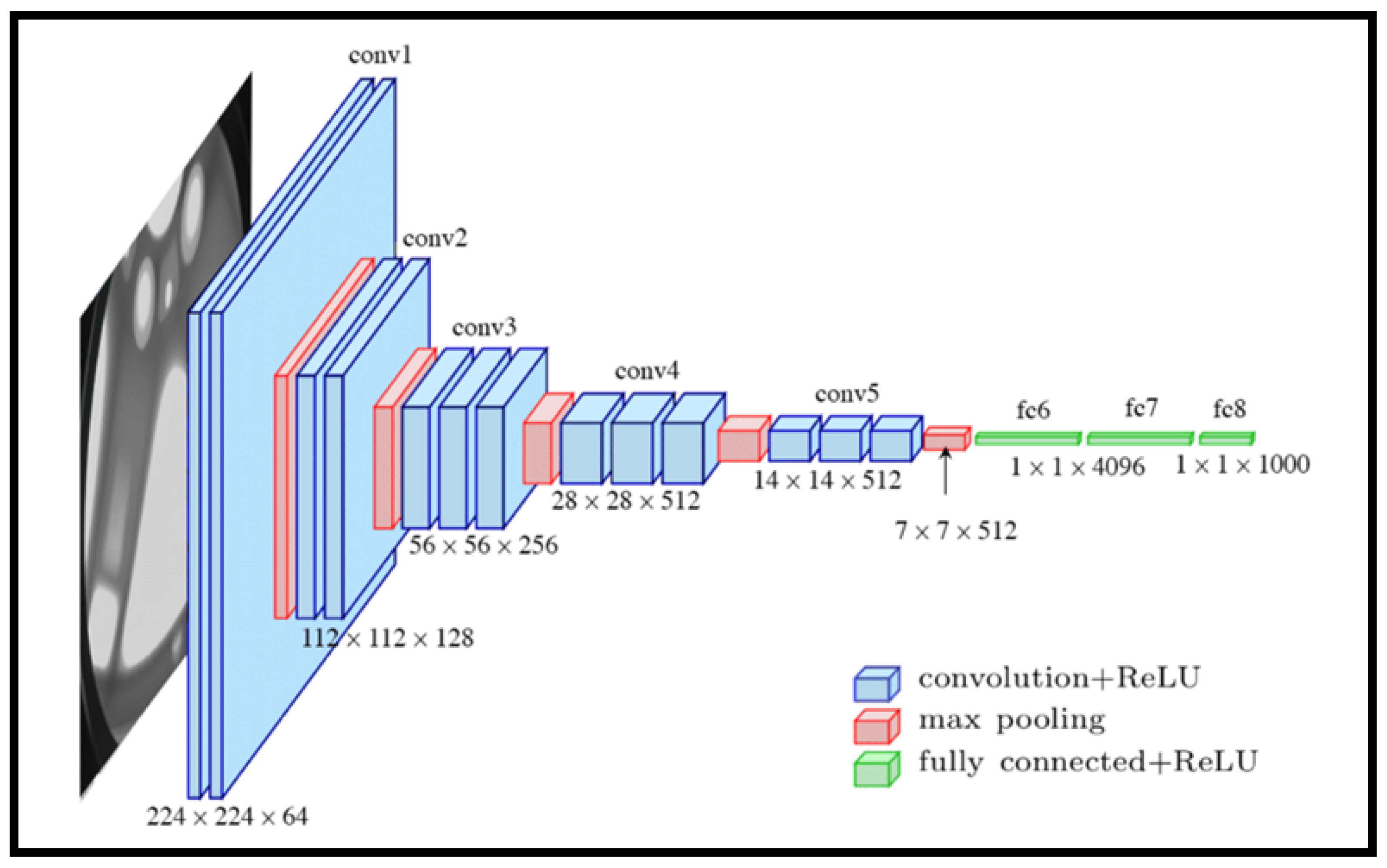
In this paper, many deep neural networks are experimented with for feature extraction, with varying results. The following convolutional neural networks are used: VGG16, VGG19, VGGFace, and face embeddings. In convolutional neural network model type VGG16, the model was initially presented as part of the ILSVRC (ImageNet Large-Scale Visual Recognition Challenge), an annual competition with the goal of categorizing images into 1000 potential output classes and recognizing them. The VGG16 CNN is composed of 16 layers, 13 of which are convolutional layers, and the final 3 are dense layers. All of the VGG16 kernels (filters) have padding of one pixel and a stride of one, whereas the pooling layers have padding of two pixels and a stride of two [34,35,36]. Figure 2 illustrates the architecture of the VGG16 network.
In a convolutional neural network model like VGG16, characteristics can be extracted from photos and categorized into several categories, although it is primarily used to assign images to one of 1000 categories. To accomplish this, the dense layers are removed, leaving only the convolutional layers to extract characteristics from the pictures. Then, a neural network or other machine learning model can be trained using those attributes to categorize a separate collection of images.
A convolutional neural network model like VGG19, it includes 19 layers, comprising 1 softmax layer, 5 max-pooling levels, 3 fully connected layers, and 16 convolutional layers. The network’s name is derived from summing up the layers with learning parameters that change throughout training. These are the fully connected and convolutional layers, totaling 19 layers with adjustable parameters. Like VGG16, VGG19 uses a kernel size of 3 × 3 pixels with a stride of one and a padding of one pixel to maintain the spatial dimension of the input picture. Additionally, a 2 × 2 pixel max-pooling layer with a stride of two is employed. VGG19 achieves high accuracy in the ILSVRC because it has been trained on more than a million pictures and 138 million learning parameters [37,38]. Figure 3 illustrates the architecture of the VGG19 network.
A Siamese neural network is a distinct kind of neural network. Such a system uses two neural networks that operate concurrently and share weights. The task of such a network is to produce an output feature vector that groups photographs from the same person together while isolating images from other individuals. The input to such a network is two images, either of the same person or two distinct persons [39,40].

2.5. Classification Methods

In this paper, three main classification methods are used: SVMs, MLP, and One vs. All classifiers (using an SVM).
The Support Vector Machine (SVM) is a supervised machine learning algorithm used for classification and regression tasks. Its primary objective is to find a hyperplane that best separates data points into different classes while maximizing the margin between the two classes. A brief overview of SVM is as follows [41]:
Hyperplane: In a two-dimensional space, a hyperplane is a line that separates data into two classes. In higher dimensions, it becomes a plane or a hyperplane.
Margin: SVM aims to find the hyperplane with the maximum margin, which is the distance between the hyperplane and the nearest data points from each class. Maximizing the margin helps improve the model’s generalization and reduces overfitting.
Support Vectors: These are the data points that are closest to the hyperplane and play a crucial role in defining the margin. SVM is named after these support vectors because they support the decision boundary.
Kernel Trick: SVM can handle non-linearly separable data by mapping it into a higher-dimensional space using a kernel function (e.g., polynomial, radial basis function) without explicitly calculating the new feature vectors. This allows SVM to find a linear hyperplane in the transformed space.
C parameter: SVM has a regularization parameter, often denoted as C, which controls the trade-off between maximizing the margin and minimizing classification errors. A smaller C encourages a wider margin but may allow some misclassification, while a larger C minimizes errors but may result in a narrower margin.
Classification: In classification tasks, SVM assigns new data points to one of the two classes based on which side of the hyperplane they fall.
SVM has gained popularity due to its ability to handle high-dimensional data, work well with small to medium-sized datasets, and provide strong generalization performance. It is commonly used in various fields, including image classification, text classification, and bioinformatics.
A Multilayer Perceptron (MLP) classifier is a type of artificial neural networks used in machine learning for supervised classification tasks. It is a feedforward neural network with multiple layers of interconnected neurons (also known as nodes or units). Here is a brief description of an MLP classifier [42]:
Input Layer: The input layer of the MLP receives the features or attributes of the data. Each neuron in this layer represents a feature, and the number of neurons is equal to the number of input features.
Hidden Layers: Between the input and output layers, there can be one or more hidden layers. These layers contain neurons that process the input data through weighted connections, apply activation functions, and pass the results to the subsequent layers. The number of neurons and the number of hidden layers are hyperparameters that can be tuned during model design.
Weights and Bias: Each connection between neurons has an associated weight, which is adjusted during the training process to learn the underlying patterns in the data. Additionally, each neuron has a bias term that helps control the neuron’s activation threshold.
Activation Functions: Activation functions are applied to the weighted sum of inputs at each neuron in the hidden layers. Common activation functions include the sigmoid, hyperbolic tangent (tanh), and rectified linear unit (ReLU). Activation functions introduce non-linearity into the model, allowing it to learn complex relationships in the data.
Output Layer: The output layer of the MLP produces the final classification results. For binary classification tasks, there is typically one neuron with a sigmoid or softmax activation function to produce a probability score or class probabilities. In multi-class classification, there are as many neurons as there are classes, and softmax activation is often used to assign probabilities to each class.
Training: MLP classifiers are trained using supervised learning with labeled training data. Backpropagation is a common training algorithm that adjusts the weights and biases iteratively to minimize a loss function, such as cross-entropy, and improve the model’s ability to make accurate predictions.
Regularization: To prevent overfitting, regularization techniques like dropout, L1/L2 regularization, and early stopping can be applied to the MLP.
MLP classifiers are versatile and capable of learning complex decision boundaries, making them suitable for a wide range of tasks, including image classification, natural language processing, and various other pattern recognition tasks. However, their performance and generalization depend on the choice of architecture, hyperparameters, and the availability of sufficient training data.
One vs. All (OvA) Support Vector Machine classifiers remain a workhorse solution for facial recognition systems, particularly when dealing with multiple individuals. The approach’s elegance lies in its simplicity—rather than wrestling with a single complex model, it breaks down the recognition challenge into a series of straightforward binary classification problems. Each SVM learns to distinguish one person’s face from all others, making the system both computationally tractable and easier to maintain. However, as any practitioner knows, the devil is in the details. The method’s real-world performance hinges critically on having sufficiently diverse training data, selecting appropriate facial features, and carefully tuning those all-important SVM parameters. Recent work by Dalal et al. (2023) and Al-Dujaili (2023) [43,44] underscores how these implementation choices can make or break a facial recognition system, especially when deploying in unconstrained environments where lighting, pose, and expression vary widely. While not without its challenges, the OvA SVM approach continues to offer a compelling combination of performance and practicality for many biometric applications.
A one vs. rest classifier is a machine learning technique that fits a binary classifier to each class in the classification issue in an effort to create a multiclass classification method. Each class is treated as being positive by the One vs. All classifier, while every other class is treated as being negative. The result is a binary classifier that does a fantastic job of differentiating one class from all other classes but fails miserably at doing so among different classes. When the model is asked to provide a new classification after being trained, it then aggregates all of the classifiers it built for each class, runs them all, and outputs the classification produced by the classifier with the highest level of confidence [43,44]. While other categorization techniques might be used, the study’s suggested algorithms are emphasized for their ability to successfully increase system performance, as seen in the findings section [45,46,47]. Additionally, the CNN approach with various structures for facial recognition in mobile environments is addressed by several researchers [48,49,50]. Furthermore, different applications make use of deep learning and other deep networks within various machine learning, signal processing, and artificial intelligence systems [51,52,53,54,55].

3. Databases

The databases used in this study are the in-house database, the Labelled Faces in the Wild (LFW) database, which is a collection of face images created for the investigation of unrestricted face identification, and the Facial identification database gathered from Pinterest (Pins).

3.1. In-House Database

A database of subjects from the Computer Engineering Department is captured inside. The database consist of in-house database Types I and II. Type-I) The In-House Database with 50 Subjects: Initially, this database contains 50 subjects and 5586 images taken via a webcam without utilizing image augmentation to increase the image count per subject. Subsequently, adjustments are made to augmentation techniques, resulting in a total of 29,086 images. These new techniques encompass horizontal flipping, Contrast-Limited Adaptive Histogram Equalization (CLAHE), random modifications in brightness and contrast, Gaussian blur, PCA, Gaussian noise, JPEG compression, median blur, and interpolation. (Type-II) The In-House Database with 10 Individuals Recorded Using a High-Quality Smartphone Camera: This database comprises 24,300 images captured using a high-quality smartphone camera and includes data from 10 individuals.

3.2. Labelled Faces in the Wild (LFW) Database

The LFW database is a public database of 5749 subjects with 13,233 images. There is an average of roughly two images per subject, and 1680 subjects have two or more images, while the rest only have one image per subject. This makes it difficult to train a good model that can recognize all of the 5749 subjects. Therefore, data augmentation is used to increase the number of images per subject. The final number of images per subject after using data augmentation is 45 images per subject, resulting in a total of 258,705 images. The database is available online at the following link: https://www.kaggle.com/datasets/jessicali9530/lfw-dataset (accessed on 23 March 2023).

3.3. Pins Face Recognition Database

The Pins database is a freely accessible online database. The Facial Recognition Dataset is collected from Pinterest. There are 105 subjects and 17,534 photos in all. It is unnecessary to apply data augmentation to enhance the number of samples per subject because this database includes a reasonably high number of photos per subject (around 167 images per person). The database is available online at the following link: https://www.kaggle.com/datasets/hereisburak/pins-face-recognition (accessed on 26 March 2023).

3.4. Training Process and Data Splitting

Three categories of data are created: validation, training, and testing. Specifically, 25% of the data are utilized for testing, 67.5% are used for training, and 7.5% are used for validation. To verify that the split is equitable for all facial recognition techniques, a random seed is used.
The details of the settings of training for each database are as follows:
In-house database (50 subjects): The images are resized to be of size 100 × 100 pixels. The OvR settings used here are the same as those for the LFW and Pins databases. The MLP used has three hidden layers (192-256-128), and the network is trained for 100 epochs with a batch size of 32.
LFW database: The images are resized to be of size 100 × 100 pixels, and an OvR classifier with an SVM as an estimator is utilized. To obtain the best outcome feasible, the SVM employs the radial basis kernel with an unlimited number of iterations.
Pins database: The images are resized to be of size 160 × 160 pixels, and an OvR classifier is used with an SVM as an estimator. The SVM also uses the radial basis kernel with an unlimited number of iterations.

4. Experimental Results and Discussion

Two major experiments have been completed for this paper. Two classifiers, MLP and SVM, are used in Experiment 1 to apply thorough evaluations of ten feature extraction techniques (SIFT, SURF, GIST, LBP, WLD, HOG, VGG16, VGG19, VGG face, and face embeddings) utilizing full faces and face modalities from the in-house database.
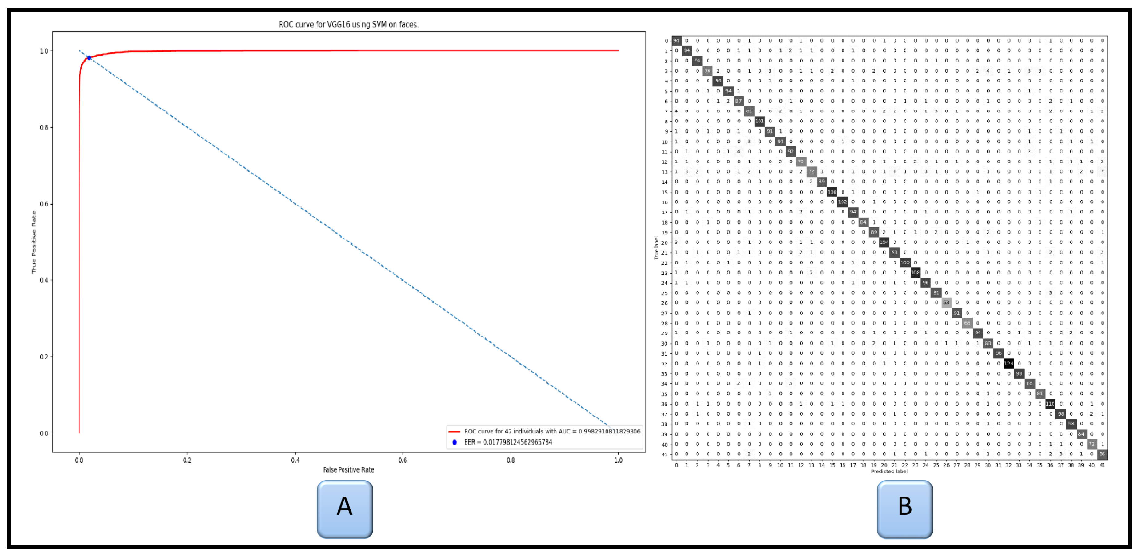
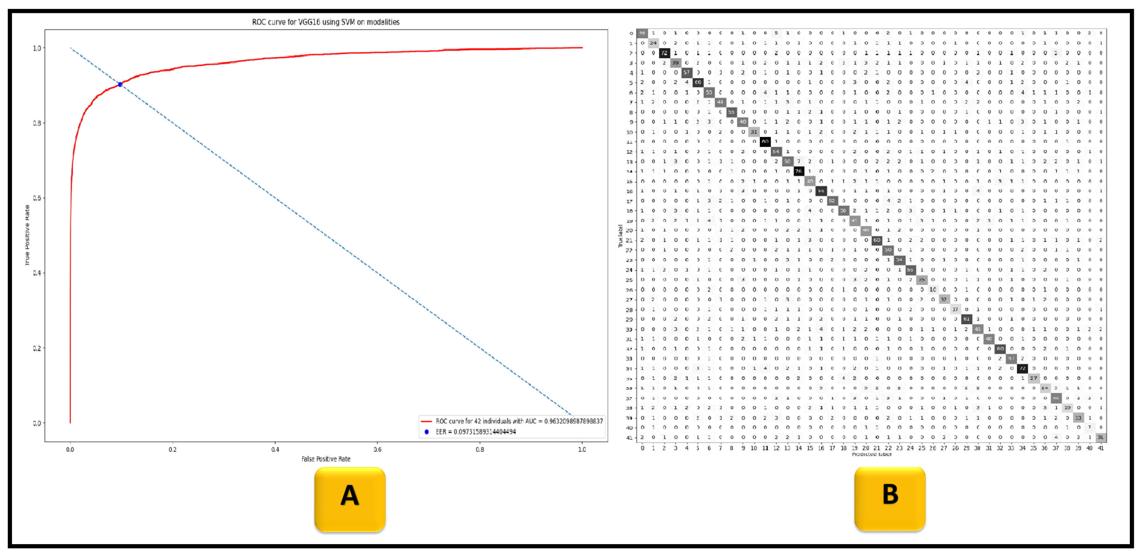
In Part (1) of Experiment 1, we exploited only 42 subjects obtained from an HD camera, with a total of 1118 images and an average of roughly 27 images per subject. The final database after data augmentation has 103,803 total images and an average of roughly 2471 images per subject. Figure 4, Figure 5, Figure 6 and Figure 7 show the best results obtained from the extracted features using the VGG16 model of the in-house dataset. Figure 4 part (A) illustrates the Receiver Operating Characteristic (ROC) curve of SVM classifier applied on the extracted feature of the whole face, while Part (B) represents the confusion matrix (CM). Figure 5 shows the result of utilizing MLP classifier applied on the extracted features of the whole face. Figure 6 shows the result utilizing the SVM classifier applied on the extracted feature of the facial modality. Figure 7 shows the result of the MLP classifier utilized on the extracted feature of the facial modality.
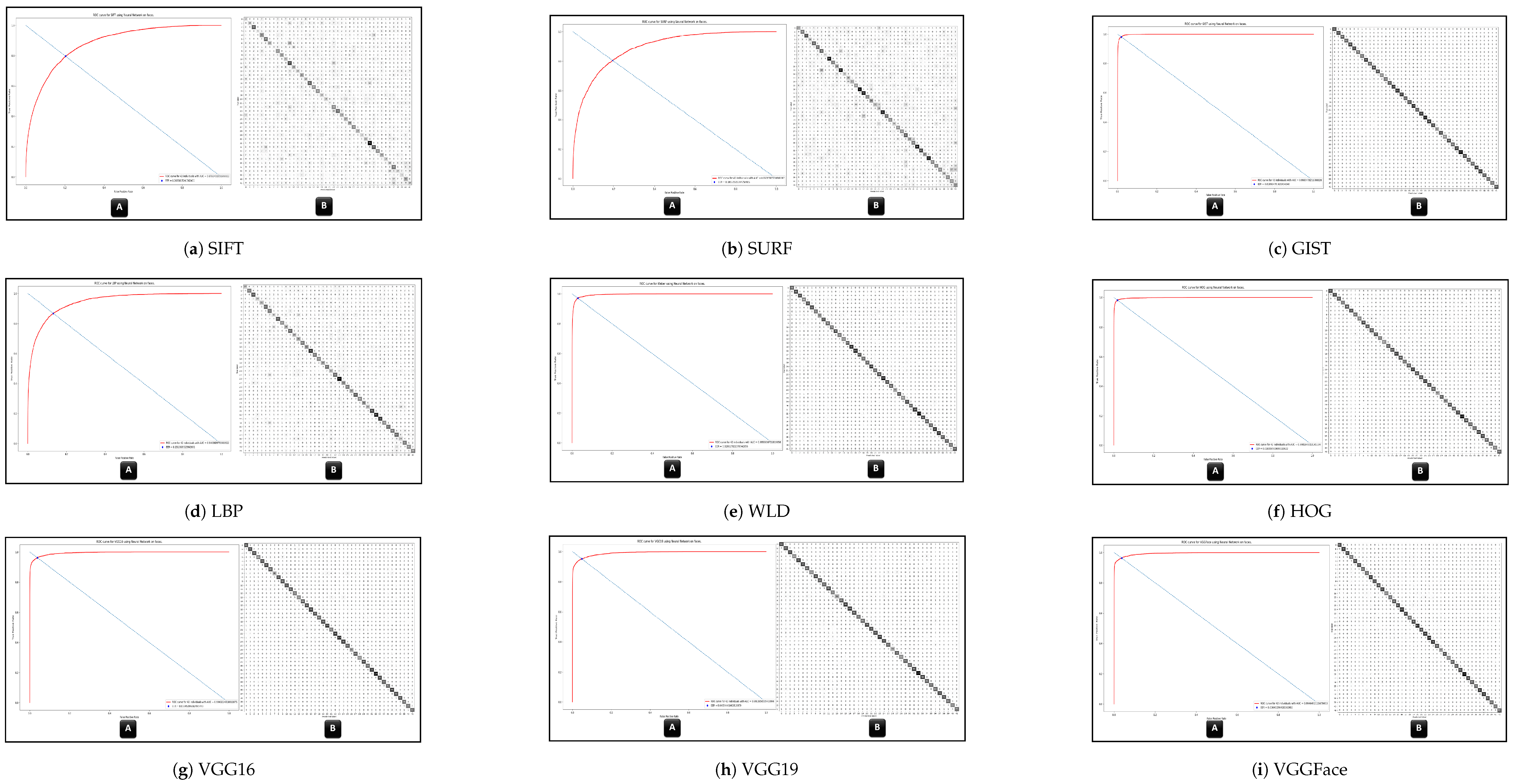
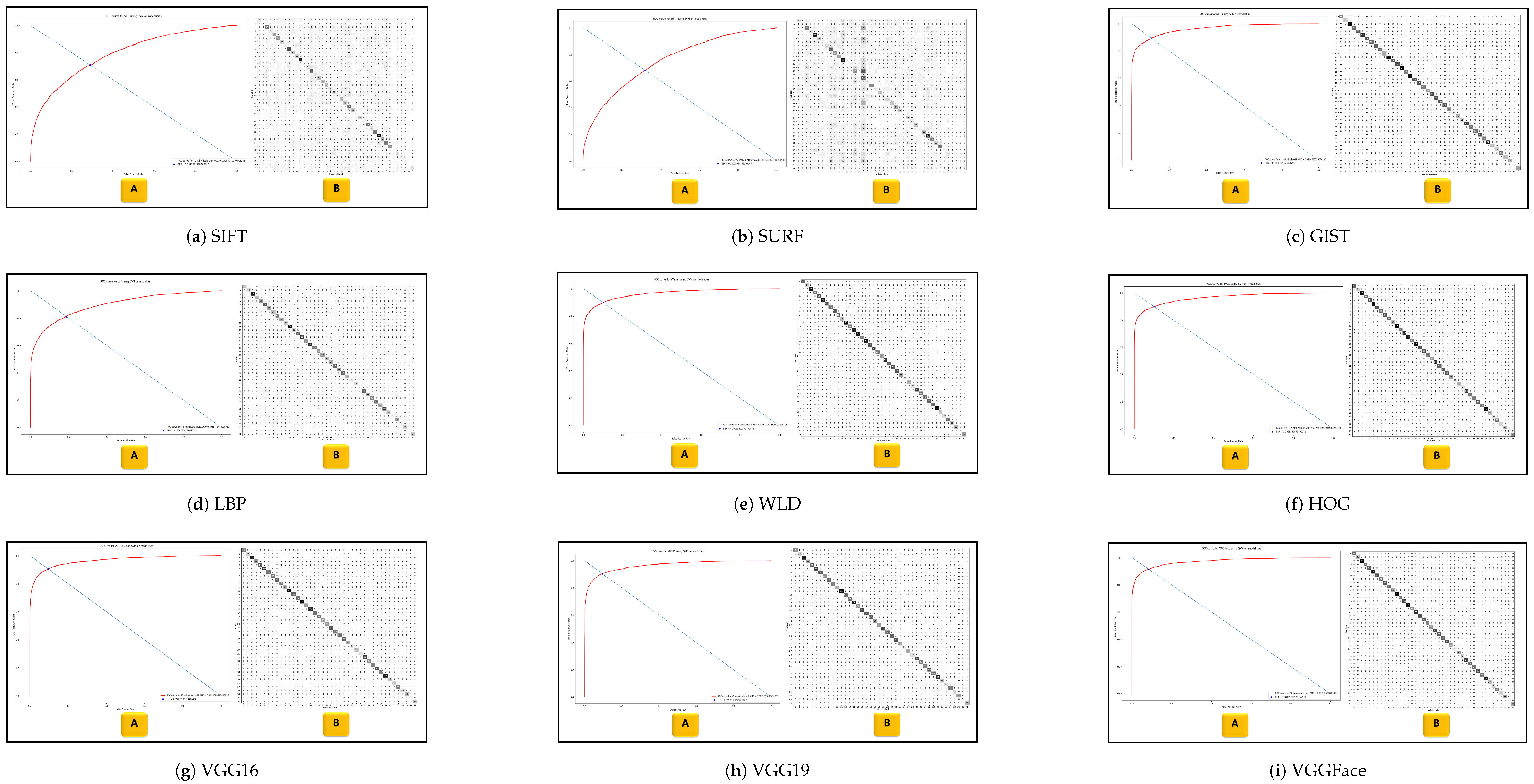
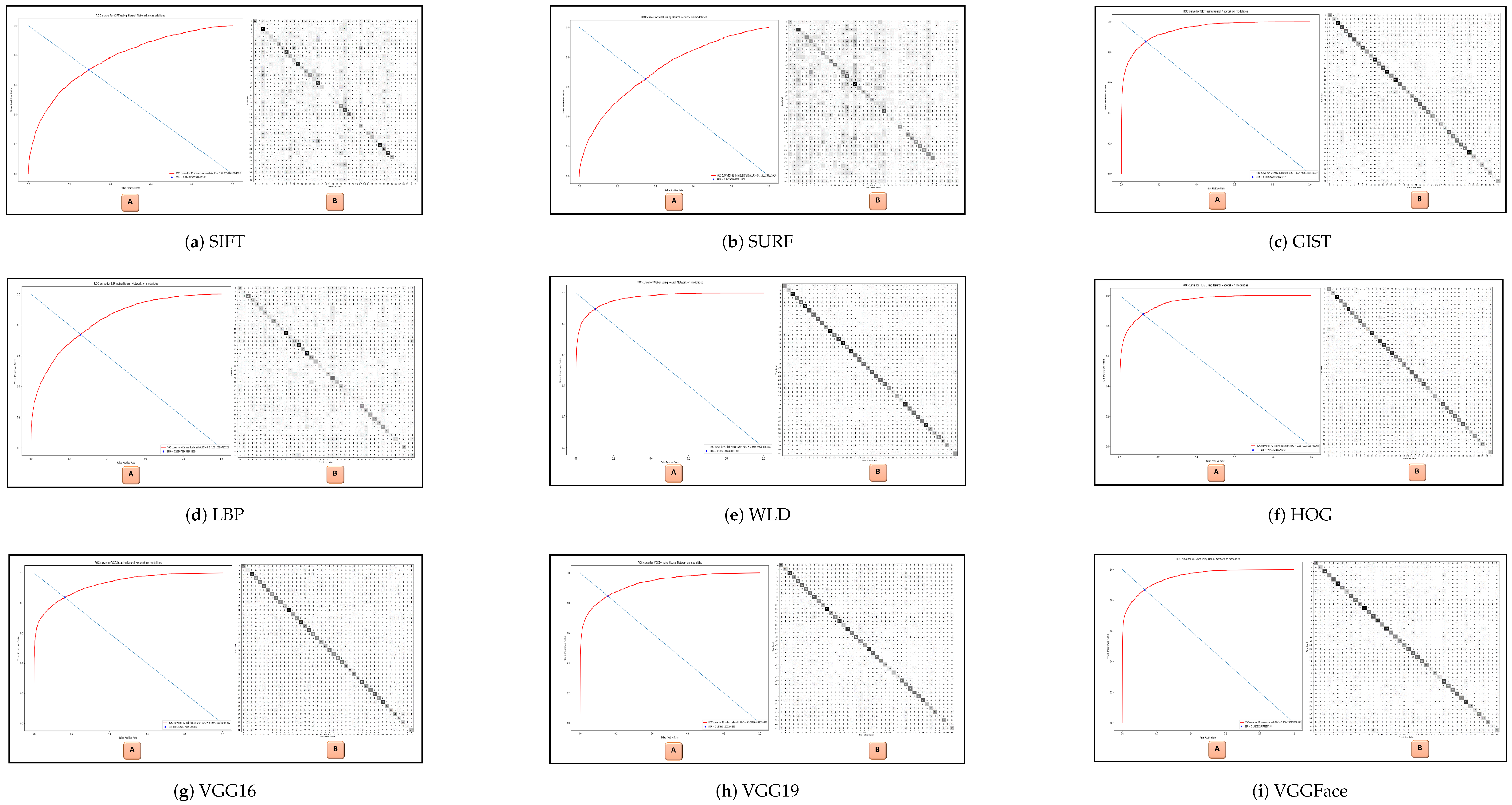
Appendix A shows all figures from Figure A1, Figure A2, Figure A3 and Figure A4. These figures show the reported result of two classifiers, namely SVM and MLP, which was applied on extracted feature methods SIFT, SURF, GIST, LBP, WLD, HOG, VGG16, VGG19, and VGGFace. All these extraction methods were obtained from the whole face and facial modalities using the in-house dataset.
In Part (2) of Experiment 1, we employ 50 subjects from the in-house database, comprising a total of 5586 images, without employing any image augmentation techniques to augment the number of images per subject. However, slight modifications have been made to the image augmentation process to yield the following results. The revised total number of samples now amounts to 29,086 images.
Table 1 shows the results of accuracies for the ten feature extraction methods. According to Table 1, GIST features have a better descriptor in terms of performance accuracy of face recognition compared to both SIFT and SURF. In addition, the HOG descriptor is invariant to lighting changes due to the normalization process described earlier, and it is faster than the Weber descriptor while being as accurate or even more accurate than both the Weber and LBP descriptors. Furthermore, VGG16 gives a higher performance accuracy compared with all other features, with 98.8% for the whole face for SVM.
In Experiment 2, we are utilizing the MLP and One vs. All SVM classifiers for the LFW and Pins databases. We are also employing the optimal feature extraction technique (VGG16) discovered in Experiment 1. In terms of Experiment 2, the system performance for the proposed VGG feature is presented in Table 2 by using SVM One vs. All MLP classifiers for both the Pins and LFW databases. According to Table 2, the LFW database achieves higher system performance than the Pins database. We show all the statistical equations related to Table 2 below.
P r e c i s i o n = T P T P + F P
R e c a l l = T P T P + F N
F 1 = 2 P r e c i s i o n R e c a l l P r e c i s i o n + R e c a l l
A c c u r a c y = T P + T N T P + T N + F P + F N
where: True Positives (TP) are the number of correctly predicted positive instances. True Negatives (TN) are the number of correctly predicted negative instances. False Positives (FP) are the number of negative instances wrongly predicted as positive. False Negatives (FN) are the number of positive instances wrongly predicted as negative.
Table 3 explains the comparison of the proposed approach with other state-of-the-art work. In addition, it is clear from Table 3 that our proposed system outperforms all other previous works.

5. Conclusions

Two significant experiments were conducted for this paper. In Experiment 1, two classifiers, MLP and SVM, were employed to conduct comprehensive evaluations of ten feature extraction techniques (SIFT, SURF, GIST, LBP, WLD, HOG, VGG16, VGG19, VGG face, and face embeddings) using full faces and face modalities from the in-house database. In Experiment 2, the MLP and One vs. All SVM classifiers were employed to evaluate the LFW and Pins databases, utilizing the optimal feature extraction technique (VGG16) identified in Experiment 1. These comprehensive evaluations, which encompassed ten feature extraction methods, served as a benchmark for other researchers interested in this field. The main conclusions can be summarized as follows.
Firstly, in terms of the in-house database, the findings above did not include Dlib’s face embedding results for facial modalities since the face embedding API required that face detection be feasible on the input picture and facial modalities were images of sections of the face rather than the complete face. Using a CNN for feature extraction and an SVM as a classifier often yielded the best results. Additionally, using the full face rather than just the face’s modality for feature extraction yielded considerably better results. The best outcome was obtained when the full face was utilized as the input to the model and VGG16 was used as a feature extractor and an SVM as a classifier. As noted in the results section, the best performance accuracy among the ten proposed feature extraction methods applied to the in-house database for the facial recognition task was 99.8%, achieved by the VGG16 model combined with the SVM classifier.
Secondly, in terms of LFW and Pins databases, the highest accuracy achieved was 99.7% by evaluating the LFW database using the SVM One vs. All classifier, while the performance accuracy was slightly less than 99.5% by using the MLP classifier for the same database (LFW). However, the performance was lower when the system was evaluated by the Pins database.

6. Data and Code Availability

The in-house data and the code provided in this study can be accessed from https://github.com/Thoalfeqar-gata/Face-recognition-on-low-powered-devices (accessed on 6 August 2024).

Author Contributions

Conceptualization, T.G.J., M.T.S.A.-K., and A.S.M.; methodology, T.G.J., M.T.S.A.-K., and A.S.M.; software, T.G.J., M.T.S.A.-K., and A.S.M.; validation, T.G.J., M.T.S.A.-K., and A.S.M.; formal analysis, T.G.J., M.T.S.A.-K., and A.S.M.; investigation, T.G.J., M.T.S.A.-K., and A.S.M.; resources, A.S.M., M.T.S.A.-K., and J.A.A.-A.; data curation, A.S.M., M.T.S.A.-K., and J.A.A.-A.; writing—original draft preparation, M.T.S.A.-K. and A.S.M.; writing—review and editing, M.T.S.A.-K. and A.S.M.; visualization, A.S.M., M.T.S.A.-K., and T.G.J.; supervision, A.S.M.; project administration, A.S.M.; No fund was provide for this research. It was a standalone research done by the authors. All authors have read and agreed to the published version of the manuscript.

Funding

This research received no external funding.

Acknowledgments

The authors would like to thank the Department of Computer Engineering, and the Department of Electrical Engineering at Mustansiriyah University, College of Engineering, Baghdad, Iraq, for their constant support and encouragement.

Conflicts of Interest

The authors declare no conflicts of interest.

Appendix A

Figure A1. Utilizing the SVM classifier applied on the extracted features of the whole face using an in-house database. (a) SIFT, (b) SURF, (c) GIST, (d) LBP, (e) WLD, (f) HOG, (g) VGG16, (h) VGG19, (i) VGGFace. Each sub-figure is categorized into two parts: part (A) ROC curve and part (B) confusion matrix.
Signals 06 00049 g0a1
Figure A2. Utilizing the MLP classifier applied on the extracted features of the whole face using an in-house database. (a) SIFT, (b) SURF, (c) GIST, (d) LBP, (e) WLD, (f) HOG, (g) VGG16, (h) VGG19, (i) VGGFace. Each sub-figure is categorized into two parts: part (A) ROC curve and part (B) confusion matrix.
Signals 06 00049 g0a2
Figure A3. Utilizing the SVM classifier applied on the extracted features of the facial modalities using an in-house database. (a) SIFT, (b) SURF, (c) GIST, (d) LBP, (e) WLD, (f) HOG, (g) VGG16, (h) VGG19, (i) VGGFace. Each sub-figure is categorized into two parts: part (A) ROC curve and part (B) confusion matrix.
Signals 06 00049 g0a3
Figure A4. Utilizing the MLP classifier applied on the extracted features of the facial modalities using an in-house database. (a) SIFT, (b) SURF, (c) GIST, (d) LBP, (e) WLD, (f) HOG, (g) VGG16, (h) VGG19, (i) VGGFace. Each sub-figure is categorized into two parts: part (A) ROC curve and part (B) confusion matrix.
Signals 06 00049 g0a4

References

  1. Walker, D.L.; Palermo, R.; Callis, Z.; Gignac, G.E. The association between intelligence and face processing abilities: A conceptual and meta-analytic review. Intelligence 2023, 96, 101718. [Google Scholar] [CrossRef]
  2. Gignac, G.E.; Shankaralingam, M.; Walker, K.; Kilpatrick, P. Short-term memory for faces relates to general intelligence moderately. Intelligence 2016, 57, 96–104. [Google Scholar] [CrossRef]
  3. Hildebrandt, A.; Sommer, W.; Schacht, A.; Wilhelm, O. Perceiving and remembering emotional facial expressions—A basic facet of emotional intelligence. Intelligence 2015, 50, 52–67. [Google Scholar] [CrossRef]
  4. Tomar, V.; Kumar, N.; Srivastava, A.R. Single sample face recognition using deep learning: A survey. Artif. Intell. Rev. 2023, 56, 1063–1111. [Google Scholar] [CrossRef]
  5. Hasan, M.R.; Guest, R.; Deravi, F. Presentation-Level Privacy Protection Techniques for Automated Face Recognition-A Survey. Acm Comput. Surv. 2023, 56, 1–27. [Google Scholar] [CrossRef]
  6. Jing, Y.; Lu, X.; Gao, S. 3D face recognition: A comprehensive survey in 2022. Comput. Vis. Media 2023, 9, 657–685. [Google Scholar] [CrossRef]
  7. Kolf, J.N.; Boutros, F.; Elliesen, J.; Theuerkauf, M.; Damer, N.; Alansari, M.; Hay, O.A.; Alansari, S.; Javed, S.; Werghi, N.; et al. EFaR 2023: Efficient Face Recognition Competition. arXiv 2023, arXiv:2308.04168. [Google Scholar] [CrossRef]
  8. Liu, F.; Chen, D.; Wang, F.; Li, Z.; Xu, F. Deep learning based single sample face recognition: A survey. Artif. Intell. Rev. 2023, 56, 2723–2748. [Google Scholar] [CrossRef]
  9. Pattnaik, I.; Dev, A.; Mohapatra, A. Forensic Facial Recognition: Review and Challenges. In Proceedings of International Conference on Data Science and Applications: ICDSA 2022; Springer: Singapore, 2023; Volume 2, pp. 351–367. [Google Scholar]
  10. Mulpuri, S.K.; Neelima, K.N.L.; Lakshmi, D.G.; Anuradha, T.; Gudapati, G.; Bulla, S. Review Paper on Facial Recognition Techniques. In Proceedings of the 2023 International Conference on Computer Communication and Informatics (ICCCI), Coimbatore, India, 23–25 January 2023; IEEE: Piscataway, NJ, USA, 2023; pp. 1–4. [Google Scholar]
  11. Shree, M.; Dev, A.; Mohapatra, A. Review on Facial Recognition System: Past, Present, and Future. In Proceedings of International Conference on Data Science and Applications: ICDSA 2022; Springer: Singapore, 2023; Volume 1, pp. 807–829. [Google Scholar]
  12. Waelen, R.A. The struggle for recognition in the age of facial recognition technology. AI Ethics 2023, 3, 215–222. [Google Scholar] [CrossRef]
  13. Kamil, M.H.M.; Zaini, N.; Mazalan, L.; Ahamad, A.H. Online attendance system based on facial recognition with face mask detection. Multimed. Tools Appl. 2023, 82, 34437–34457. [Google Scholar] [CrossRef]
  14. Ikromovich, H.O.; Mamatkulovich, B.B. Facial recognition using transfer learning in the deep CNN. Open Access Repos. 2023, 4, 502–507. [Google Scholar]
  15. Dang, T.V. Smart attendance system based on improved facial recognition. J. Robot. Control (JRC) 2023, 4, 46–53. [Google Scholar] [CrossRef]
  16. Sahan, J.M.; Abbas, E.I.; Abood, Z.M. A facial recognition using a combination of a novel one dimension deep CNN and LDA. Mater. Today Proc. 2023, 80, 3594–3599. [Google Scholar] [CrossRef]
  17. Mehdizadeh, M.; Tavakoli Tafti, K.; Soltani, P. Evaluation of histogram equalization and contrast limited adaptive histogram equalization effect on image quality and fractal dimensions of digital periapical radiographs. Oral Radiol. 2023, 39, 418–424. [Google Scholar] [CrossRef]
  18. Rahman, H.; Paul, G.C. Tripartite sub-image histogram equalization for slightly low contrast gray-tone image enhancement. Pattern Recognit. 2023, 134, 109043. [Google Scholar] [CrossRef]
  19. Younus, S.M.; Bhardwaj, V.; Jain, A.; Sharma, V.; Reddy, T.J.; Virender. A Comparative Analysis of Face Detection Algorithms and Real-Time Facial Recognition. In Proceedings of the 2023 5th International Conference on Inventive Research in Computing Applications (ICIRCA), Coimbatore, India, 3–5 August 2023; IEEE: Piscataway, NJ, USA, 2023; pp. 173–177. [Google Scholar]
  20. Bedair, A.; Abdel-Nasser, M. Gamma Effect in Face Detection Methods. SVU-Int. J. Eng. Sci. Appl. 2023, 4, 79–84. [Google Scholar]
  21. Khan, S.S.; Sengupta, D.; Ghosh, A.; Chaudhuri, A. MTCNN++: A CNN-based face detection algorithm inspired by MTCNN. Vis. Comput. 2023, 40, 899–917. [Google Scholar] [CrossRef]
  22. Abdullah, M.T.; Ali, N.H.M. Deploying Facial Segmentation Landmarks for Deepfake Detection. J. Al-Qadisiyah Comput. Sci. Math. 2023, 15, 137–149. [Google Scholar] [CrossRef]
  23. Challa, N.P.; Krishna, E.P.; Chakravarthi, S.S. Facial Landmarks Detection System with OpenCV Mediapipe and Python using Optical Flow (Active) Approach. In Proceedings of the 2023 3rd International Conference on Advance Computing and Innovative Technologies in Engineering (ICACITE), Greater Noida, India, 12–13 May 2023; IEEE: Piscataway, NJ, USA, 2023; pp. 92–96. [Google Scholar]
  24. Anami, B.S.; Sagarnal, C.V. A fusion of hand-crafted features and deep neural network for indoor scene classification. Malays. J. Comput. Sci. 2023, 36, 193–207. [Google Scholar] [CrossRef]
  25. Benjdira, B.; Ali, A.M.; Koubaa, A. Streamlined Global and Local Features Combinator (SGLC) for High Resolution Image Dehazing. In Proceedings of the IEEE/CVF Conference on Computer Vision and Pattern Recognition, Vancouver, BC, Canada, 17–24 June 2023; pp. 1854–1863. [Google Scholar]
  26. Selvi, A.; Thilagamani, S. Scale Invariant Feature Transform with Crow Optimization for Breast Cancer Detection. Intell. Autom. Soft Comput. 2023, 36, 2973–2987. [Google Scholar] [CrossRef]
  27. Anzid, H.; le Goic, G.; Bekkari, A.; Mansouri, A.; Mammass, D. A new SURF-based algorithm for robust registration of multimodal images data. Vis. Comput. 2023, 39, 1667–1681. [Google Scholar] [CrossRef]
  28. Raat, E.; Kyle-Davidson, C.; Evans, K. Using global feedback to induce learning of gist of abnormality in mammograms. Cogn. Res. Princ. Implic. 2023, 8, 1–22. [Google Scholar] [CrossRef] [PubMed]
  29. Karanwal, S.; Diwakar, M. Triangle and orthogonal local binary pattern for face recognition. Multimed. Tools Appl. 2023, 82, 36179–36205. [Google Scholar] [CrossRef]
  30. He, S.; Xie, Y.; Yang, Z. High-boost-based local Weber contrast method for infrared small target detection. Remote Sens. Lett. 2023, 14, 103–113. [Google Scholar] [CrossRef]
  31. Bhattarai, B.; Subedi, R.; Gaire, R.R.; Vazquez, E.; Stoyanov, D. Histogram of Oriented Gradients meet deep learning: A novel multi-task deep network for 2D surgical image semantic segmentation. Med. Image Anal. 2023, 85, 102747. [Google Scholar] [CrossRef] [PubMed]
  32. Kumar, C.R.; Saranya, N.; Priyadharshini, M.; Gilchrist, D.; Rahman, M.K. Face recognition using CNN and siamese network. Meas. Sensors 2023, 27, 100800. [Google Scholar] [CrossRef]
  33. Ean, I.C.K.; Abu Hassan, M.F.; Yusof, Y.; Nadzri, N.Z. Deep CNN-Based Facial Recognition for a Person Identification System Using the Inception Model. In Industrial Revolution in Knowledge Management and Technology; Springer: Berlin/Heidelberg, Germany, 2023; pp. 85–95. [Google Scholar]
  34. Mishra, R.; Wadekar, S.; Warbhe, S.; Dalal, S.; Mirajkar, R.; Sathe, S. Facial Recognition System Using Transfer Learning with the Help of VGG16. In AI, IoT, Big Data and Cloud Computing for Industry 4.0; Springer: Berlin/Heidelberg, Germany, 2023; pp. 163–180. [Google Scholar]
  35. Bewoor, M.; Patil, S.; Kushwaha, S.; Tandon, S.; Trivedi, S.; Pawar, A. Face recognition using open CV and VGG 16 transfer learning. Aip Conf. Proc. 2023, 2890, 020019. [Google Scholar]
  36. Khajuria, O.; Kumar, R.; Gupta, M. Facial Emotion Recognition using CNN and VGG-16. In Proceedings of the 2023 International Conference on Inventive Computation Technologies (ICICT), Lalitpur, Nepal, 26–28 April 2023; IEEE: Piscataway, NJ, USA, 2023; pp. 472–477. [Google Scholar]
  37. Melinda, M.; Oktiana, M.; Nurdin, Y.; Pujiati, I.; Irhamsyah, M.; Basir, N. Performance of ShuffleNet and VGG-19 Architectural Classification Models for Face Recognition in Autistic Children. Int. J. Adv. Sci. Eng. Inf. Technol. 2023, 13, 674–680. [Google Scholar] [CrossRef]
  38. Vignesh, S.; Savithadevi, M.; Sridevi, M.; Sridhar, R. A novel facial emotion recognition model using segmentation VGG-19 architecture. Int. J. Inf. Technol. 2023, 15, 1777–1787. [Google Scholar] [CrossRef]
  39. Chakraborty, U.K.; Bendre, A.; Ganguli, S.; Rai, R.N. Prosthetic Face Recognition using a Siamese Neural Network Approach. In Proceedings of the 2023 4th International Conference on Computing and Communication Systems (I3CS), Shillong, India, 16–18 March 2023; IEEE: Piscataway, NJ, USA, 2023; pp. 1–6. [Google Scholar]
  40. Khan, M.; Saeed, M.; El Saddik, A.; Gueaieb, W. ARTriViT: Automatic Face Recognition System Using ViT-Based Siamese Neural Networks with a Triplet Loss. In Proceedings of the 2023 IEEE 32nd International Symposium on Industrial Electronics (ISIE), Helsinki, Finland, 19–21 June 2023; IEEE: Piscataway, NJ, USA, 2023; pp. 1–6. [Google Scholar]
  41. Traore, M.M.; Traore, D. Face Recognition efficiency Based on Support Vector Machine using Skin Color Information. Maghrebian J. Pure Appl. Sci. 2023, 9. [Google Scholar]
  42. Jamali, A.; Mahdianpari, M.; Abdul Rahman, A. Hyperspectral image classification using multi-layer perceptron mixer (MLP-MIXER). Int. Arch. Photogramm. Remote Sens. Spat. Inf. Sci. 2023, 48, 179–182. [Google Scholar] [CrossRef]
  43. Dalal, T.; Yadav, J. Large-scale orthogonal integer wavelet transform features-based active support vector machine for multi-class face recognition. Int. J. Comput. Appl. Technol. 2023, 72, 108–124. [Google Scholar] [CrossRef]
  44. Al_Dujaili, M.J.; Salim ALRikabi, H.T.; Abed, N.K.; Niama ALRubeei, I.R. Gender Recognition of Human from Face Images Using Multi-Class Support Vector Machine (SVM) Classifiers. Int. J. Interact. Mob. Technol. 2023, 17, 113–134. [Google Scholar] [CrossRef]
  45. Al-Kaltakchi, M.T.; Woo, W.L.; Dlay, S.S.; Chambers, J.A. Multi-dimensional i-vector closed set speaker identification based on an extreme learning machine with and without fusion technologies. In Proceedings of the 2017 Intelligent Systems Conference (IntelliSys), London, UK, 7–8 September 2017; IEEE: Piscataway, NJ, USA, 2017; pp. 1141–1146. [Google Scholar]
  46. Al-Kaltakchi, M.T.S. Robust Text Independent Closed Set Speaker Identification Systems and Their Evaluation. Ph.D. Thesis, Newcastle University, Newcastle upon Tyne, UK, 2018. [Google Scholar]
  47. Al-Kaltakchi, M.T.S.; Al-Sumaidaee, S.A.M.; Al-Nima, R.R.O. Classifications of signatures by radial basis neural network. Bull. Electr. Eng. Inform. 2022, 11, 3294–3300. [Google Scholar] [CrossRef]
  48. Mohammad, A.S. Multi-Modal Ocular Recognition in Presence of Occlusion in Mobile Devices; University of Missouri-Kansas City: Kansas City, MO, USA, 2018. [Google Scholar]
  49. Mohammad, A.S.; Al-Ani, J.A. Convolutional neural network for ethnicity classification using ocular region in mobile environment. In Proceedings of the 2018 10th Computer Science and Electronic Engineering (CEEC), Colchester, UK, 19–21 September 2018; IEEE: Piscataway, NJ, USA, 2018; pp. 293–298. [Google Scholar]
  50. Mohammad, A.S.; Rattani, A.; Derakhshani, R. Comparison of squeezed convolutional neural network models for eyeglasses detection in mobile environment. J. Comput. Sci. Coll. 2018, 33, 136–144. [Google Scholar]
  51. Mohammad, A.S.; Al-Kaltakchi, M.T.; Alshehabi Al-Ani, J.; Chambers, J.A. Comprehensive Evaluations of Student Performance Estimation via Machine Learning. Mathematics 2023, 11, 3153. [Google Scholar] [CrossRef]
  52. Al-Kaltakchi, M.T.; Mohammad, A.S.; Woo, W.L. Ensemble System of Deep Neural Networks for Single-Channel Audio Separation. Information 2023, 14, 352. [Google Scholar] [CrossRef]
  53. Al-Nima, R.R.O.; Al-Kaltakchi, M.T.; Han, T.; Woo, W.L. Road tracking enhancements for self-driving cars applications. Aip Conf. Proc. 2023, 2839, 040004. [Google Scholar]
  54. Devnath, L.; Arora, P.; Carraro, A.; Korbelik, J.; Keyes, M.; Wang, G.; Guillaud, M.; MacAulay, C. Recognizing Epithelial Cells in Prostatic Glands Using Deep Learning. Cells 2025, 14, 737. [Google Scholar] [CrossRef] [PubMed]
  55. Yuan, R.; Janzen, I.; Devnath, L.; Khattra, S.; Myers, R.; Lam, S.; MacAulay, C. MA19. 11 Predicting Future Lung Cancer Risk with Low-Dose Screening CT Using an Artificial Intelligence Model. J. Thorac. Oncol. 2023, 18, S174. [Google Scholar] [CrossRef]
  56. Deng, W.; Hu, J.; Zhang, N.; Chen, B.; Guo, J. Fine-grained face verification: FGLFW database, baselines, and human-DCMN partnership. Pattern Recognit. 2017, 66, 63–73. [Google Scholar] [CrossRef]
  57. Masud, M.; Muhammad, G.; Alhumyani, H.; Alshamrani, S.S.; Cheikhrouhou, O.; Ibrahim, S.; Hossain, M.S. Deep learning-based intelligent face recognition in IoT-cloud environment. Comput. Commun. 2020, 152, 215–222. [Google Scholar] [CrossRef]
  58. Zhao, Y.; Deng, W. Dual Gaussian Modeling for Deep Face Embeddings. Pattern Recognit. Lett. 2022, 161, 74–81. [Google Scholar] [CrossRef]
  59. Dastmalchi, H.; Aghaeinia, H. Super-resolution of very low-resolution face images with a wavelet integrated, identity preserving, adversarial network. Signal Process. Image Commun. 2022, 107, 116755. [Google Scholar] [CrossRef]
  60. Ding, C.; Tao, D. Robust face recognition via multimodal deep face representation. IEEE Trans. Multimed. 2015, 17, 2049–2058. [Google Scholar] [CrossRef]
  61. Deng, J.; Zhou, Y.; Zafeiriou, S. Marginal loss for deep face recognition. In Proceedings of the IEEE Conference on Computer Vision and Pattern Recognition Workshops, Honolulu, HI, USA, 21–26 July 2017; pp. 60–68. [Google Scholar]
  62. Chen, J.; Chen, J.; Wang, Z.; Liang, C.; Lin, C.W. Identity-aware face super-resolution for low-resolution face recognition. IEEE Signal Process. Lett. 2020, 27, 645–649. [Google Scholar] [CrossRef]
  63. Liu, J.; Deng, Y.; Bai, T.; Wei, Z.; Huang, C. Targeting ultimate accuracy: Face recognition via deep embedding. arXiv 2015, arXiv:1506.07310. [Google Scholar] [CrossRef]
  64. Wu, W.; Kan, M.; Liu, X.; Yang, Y.; Shan, S.; Chen, X. Recursive spatial transformer (rest) for alignment-free face recognition. In Proceedings of the IEEE International Conference on Computer Vision, Venice, Italy, 22–29 October 2017; pp. 3772–3780. [Google Scholar]
  65. Rong, C.; Zhang, X.; Lin, Y. Feature-improving generative adversarial network for face frontalization. IEEE Access 2020, 8, 68842–68851. [Google Scholar] [CrossRef]
  66. Huang, G.B.; Lee, H.; Learned-Miller, E. Learning hierarchical representations for face verification with convolutional deep belief networks. In Proceedings of the 2012 IEEE Conference on Computer Vision and Pattern Recognition, Providence, RI, USA, 16–21 June 2012; IEEE: Piscataway, NJ, USA, 2012; pp. 2518–2525. [Google Scholar]
  67. Sun, Y.; Wang, X.; Tang, X. Hybrid deep learning for face verification. In Proceedings of the IEEE International Conference on Computer Vision, Sydney, NSW, Australia, 1–8 December 2013; pp. 1489–1496. [Google Scholar]
  68. Sun, Y.; Liang, D.; Wang, X.; Tang, X. Deepid3: Face recognition with very deep neural networks. arXiv 2015, arXiv:1502.00873. [Google Scholar] [CrossRef]
  69. Liu, B.; Deng, W.; Zhong, Y.; Wang, M.; Hu, J.; Tao, X.; Huang, Y. Fair loss: Margin-aware reinforcement learning for deep face recognition. In Proceedings of the IEEE/CVF International Conference on Computer Vision, Seoul, Republic of Korea, 27 October–2 November 2019; pp. 10052–10061. [Google Scholar]
  70. Sun, Y.; Wang, X.; Tang, X. Hybrid deep learning for computing face similarities. In Proceedings of the International Conference on Computer Vision (ICCV), Sydney, Australia, 1–8 December 2013; Volume 1. [Google Scholar]
  71. Guo, K.; Wu, S.; Xu, Y. Face recognition using both visible light image and near-infrared image and a deep network. CAAI Trans. Intell. Technol. 2017, 2, 39–47. [Google Scholar] [CrossRef]
  72. Lu, Z.; Jiang, X.; Kot, A. Deep coupled resnet for low-resolution face recognition. IEEE Signal Process. Lett. 2018, 25, 526–530. [Google Scholar] [CrossRef]
  73. Taigman, Y.; Yang, M.; Ranzato, M.; Wolf, L. Deepface: Closing the gap to human-level performance in face verification. In Proceedings of the IEEE Conference on Computer Vision and Pattern Recognition, Columbus, OH, USA, 23–28 June 2014; pp. 1701–1708. [Google Scholar]
  74. Sun, Y.; Wang, X.; Tang, X. Deep learning face representation from predicting 10,000 classes. In Proceedings of the IEEE Conference on Computer Vision and Pattern Recognition, Columbus, OH, USA, 23–28 June 2014; pp. 1891–1898. [Google Scholar]
  75. Sun, Y.; Wang, X.; Tang, X. Deeply learned face representations are sparse, selective, and robust. In Proceedings of the IEEE Conference on Computer Vision and Pattern Recognition, Boston, MA, USA, 7–12 June 2015; pp. 2892–2900. [Google Scholar]
  76. Parkhi, O.; Vedaldi, A.; Zisserman, A. Deep face recognition. In Proceedings of the BMVC 2015-Proceedings of the British Machine Vision Conference 2015, Swansea, UK, 7–10 September 2015; British Machine Vision Association: Durham, UK, 2015. [Google Scholar]
  77. Schroff, F.; Kalenichenko, D.; Philbin, J. Facenet: A unified embedding for face recognition and clustering. In Proceedings of the IEEE Conference on Computer Vision and Pattern Recognition, Boston, MA, USA, 7–12 June 2015; pp. 815–823. [Google Scholar]
  78. Wang, F.; Cheng, J.; Liu, W.; Liu, H. Additive margin softmax for face verification. IEEE Signal Process. Lett. 2018, 25, 926–930. [Google Scholar] [CrossRef]
  79. Wang, H.; Wang, Y.; Zhou, Z.; Ji, X.; Gong, D.; Zhou, J.; Li, Z.; Liu, W. Cosface: Large margin cosine loss for deep face recognition. In Proceedings of the IEEE Conference on Computer Vision and Pattern Recognition, Salt Lake City, UT, USA, 18–23 June 2018; pp. 5265–5274. [Google Scholar]
  80. Rajeshkumar, G.; Braveen, M.; Venkatesh, R.; Shermila, P.J.; Prabu, B.G.; Veerasamy, B.; Bharathi, B.; Jeyam, A. Smart office automation via faster R-CNN based face recognition and internet of things. Meas. Sensors 2023, 27, 100719. [Google Scholar] [CrossRef]
  81. Mahmood, B.A.; Kurnaz, S. An investigational FW-MPM-LSTM approach for face recognition using defective data. Image Vis. Comput. 2023, 132, 104644. [Google Scholar] [CrossRef]
  82. Chowdhury, P.R.; Wadhwa, A.S.; Tyagi, N. Brain inspired face recognition: A computational framework. Cogn. Syst. Res. 2023, 78, 1–13. [Google Scholar] [CrossRef]
  83. Boussaad, L.; Boucetta, A. Deep-learning based descriptors in application to aging problem in face recognition. J. King Saud Univ.-Comput. Inf. Sci. 2022, 34, 2975–2981. [Google Scholar] [CrossRef]
  84. Sikha, O.; Bharath, B. VGG16-random Fourier hybrid model for masked face recognition. Soft Comput. 2022, 26, 12795–12810. [Google Scholar] [CrossRef] [PubMed]
  85. Perdana, A.B.; Prahara, A. Face recognition using light-convolutional neural networks based on modified Vgg16 model. In Proceedings of the 2019 International Conference of Computer Science and Information Technology (ICoSNIKOM), Medan, Indonesia, 28–29 November 2019; IEEE: Piscataway, NJ, USA, 2019; pp. 1–4. [Google Scholar]
  86. Yu, J.; Sun, K.; Gao, F.; Zhu, S. Face biometric quality assessment via light CNN. Pattern Recognit. Lett. 2018, 107, 25–32. [Google Scholar] [CrossRef]
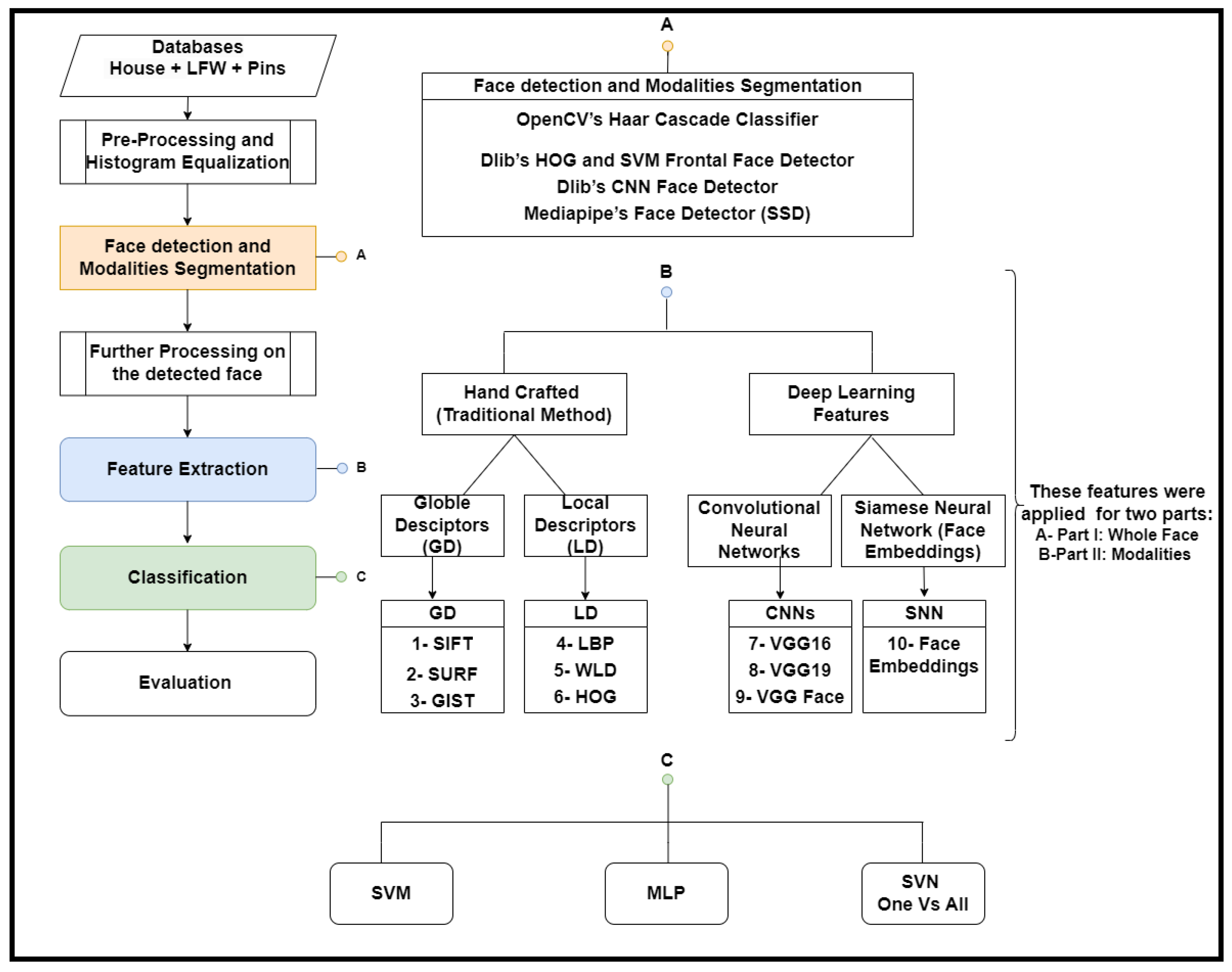
Figure 1. The structure of the facial recognition system.
Signals 06 00049 g001
Figure 2. The architecture of VGG16.
Signals 06 00049 g002
Figure 3. The architecture of VGG19.
Signals 06 00049 g003
Figure 4. The best result utilizing the SVM classifier applied on the extracted VGG16 feature of the whole face using in-house database. Part (A) ROC curve; and Part (B) confusion matrix.
Signals 06 00049 g004
Figure 5. The best result Utilizing the MLP classifier applied on the extracted VGG16 feature of the whole face using an in-house database. Part (A) ROC curve and part (B) The confusion matrix.
Signals 06 00049 g005
Figure 6. The best result Utilizing the SVM classifier applied on the extracted VGG16 feature of the facial modalities using in-house database. Part (A) ROC curve and part (B) confusion matrix.
Signals 06 00049 g006
Figure 7. The best result utilizing the MLP classifier applied on the extracted VGG16 feature of the facial modalities using in-house database. Part (A) ROC curve and part (B) confusion matrix.
Signals 06 00049 g007
Table 1. The performance accuracy for the proposed ten feature extraction methods to the in-house database based on facial recognition task using MLP and SVM classifiers.
Feature
Extractor
MLP on
Faces
MLP on
Modalities
SVM on
Faces
SVM on
Modalities
SIFT70.5%53.0%34.8%59.9%
SURF79.5%41.7%41.1%46.3%
GIST99.4%94.4%92.6%96.3%
LBP88.1%25.5%68.1%85.7%
WLD97.7%94.6%97.7%95.8%
HOG98.4%93.3%99.5%97.3%
VGG1698.2%94.0%99.8%96.4%
VGG1996.4%94.8%99.7%96.9%
VGGFace93.0%96.3%99.7%97.9%
Face embeddings46.1%None46.3%None
Table 2. The system performance (F1 score, precision, recall, accuracy) for the proposed VGG16 feature extraction method on the Pins and LFW databases using MLP and SVM One vs. All classifiers.
MethodF1 ScorePrecisionRecallAccuracyDatabase
MLP97.3%97.4%97.3%97.4%Pins
SVM O vs. All98.4%98.5%98.4%98.4%Pins
MLP99.5%99.5%99.6%99.5%LFW
SVM O vs. All99.7%99.8%99.7%99.7%LFW
Table 3. Comparison of the proposed approach with other state-of-the-art work under the same protocol.
ReferencesDatabaseModel UsedAccuracy %
[56]LFWDCMN98.03%
FGLFWDCMN91.00%
[57]LFWTree-Based Deep95.84%
FEI98.65%
ORL99.19%
[58]Training: CASIAWebFaceDGMTraining: CASIA
LFW99.27%
CFP-FF99.26%
CFP-FP86.97%
CPLF93.09%
Trained on VGG FaceTrained on VGG Face
LFW99.62%
CFP-FF99.63%
CFP-FP92.45%
CPLF96.37%
[59]LFWIPA86.10%
WIPA86.00%
[60]LFWMM-DFR99.02%
[61]LFWMarginal Loss99.48%
YTF95.98%
AgeDB98.95%
CACD95.75%
[62]LFWLight CNN98.98%
[63]LFWCNN and deep metric learning99.77%
[64]LFWReST99.03%
YTF95.40%
[65]LFWFI-GAN98.30%
CFP94.20%
[66]LFWHand-crafted and Deep learning.87.77%
[67]LFWhybrid ConvNet-RBM model92.52%
[68]LFWDeepID399.53%
[69]LFWFair loss-Cos99.53%
YTF96.20%
[70]LFWCNN-RBM93.80%
[71]LFWVGGNet98.99%
YTF97.30%
[72]LFWDeep coupled ResNet99.00%
[73]LFWDeep face97.35%
[74]LFWDeep ID97.40%
[75]LFWDeep ID299.50%
[76]LFWVGGFace98.90%
[77]LFWFaceNet99.60%
[78]LFWAMS loss, Caffe94.50%
[79]LFWCosFace99.73%
YTF97.60%
[80]NAfaster R-CNN99.30%
[81]NAFW-MPM-LSTM99.58%
[82]ORLBIFR98.50%
[83]face-aging FG-NETDeep CNN models98.21%
[84]1-Face dataset by robotics labVGG16-random Fourier hybrid model97.46%
2-Head pose image dataset97.63%
3-Georgia tech face dataset97.55%
[85]ROSE-Youtu Face Liveness Detection Database + In HouseLight-CNN Based on Modified VGG1694.40%
[86]CASIA, FLWLight CNN99.00%
ProposedHouseVGG16+SVM99.80%
ProposedHouseVGG16+MLP98.20%
ProposedLFWVGG16+SVM99.70%
ProposedLFWVGG16+MLP99.50%
ProposedPinsVGG16+SVM98.40%
ProposedPinsVGG16+MLP97.40%
Disclaimer/Publisher’s Note: The statements, opinions and data contained in all publications are solely those of the individual author(s) and contributor(s) and not of MDPI and/or the editor(s). MDPI and/or the editor(s) disclaim responsibility for any injury to people or property resulting from any ideas, methods, instructions or products referred to in the content.