Beyond Correlation: Mutual Information to Detect Damage in Nonlinear Systems

Abstract

Analyzing and measuring the similarity between two signals is a common task in many vibration-based structural health monitoring applications. Coherence between input and response signals serves as a convenient indicator of damage, based on the premise that nonlinearity due to damage in a linear system manifests as a loss of coherence in specific frequency bands. Because input excitations in civil structures are difficult to measure, damage indicators based on the coherence between two response signals have been developed. These indicators have shown promise in detecting nonlinear behavior in structures that were initially linear. This paper proposes a new damage indicator based on Mutual Information, a nonlinear extension of the squared correlation coefficient, to quantify the similarity between two signals without making assumptions about the nature of their interactions or the underlying dynamics of the system. Mutual Information is distinguished from other nonlinear similarity metrics due to its ability to capture all types of nonlinear dependencies, its high computational efficiency, and its invariance to invertible transformations, such as scaling. The proposed approach is demonstrated using a standard dataset containing experimental data from a three-story aluminum frame structure under 17 different damage states. The results show that the proposed metric can detect deviations from the baseline state due to changes in mass, stiffness, or newly induced nonlinear behavior, suggesting its potential for monitoring changes in the structural system.

1. Introduction

A key task in many existing vibration-based damage detection methods is to quantify the similarity between two signals. This comparison can be performed using the timedomain, frequency-domain, or in the joint time-frequency-domain. The similarity measure is typically derived from the concept of correlation, which quantifies the direction and strength of linear association between two data vectors. Many researchers used an extension or a variant of an autoregressive moving-average (ARMA) model of measured acceleration time histories [1,2,3,4]. While the ARMA approach is theoretically justified for the conditions assumed in its derivation, its practical applications have been limited by the implicit assumptions that the recorded time history is stationary and the system is linear before and after the damage. The first assumption renders this approach unsuitable for the detection of damages under nonstationary loads (e.g., wind and seismic loads), and the second assumption limits its applicability to a small class of damages, where the structure continues to behave in a linear fashion after damage, albeit with altered properties.

The coherence function, originally introduced by Norbert Wiener in the late 1920s [5], measures the similarity between two signals in the frequency domain. As a complex function, coherence function represents both amplitude and phase relationships between two signals. Coherence between input and response signals is a convenient indicator of damage, based on the premise that nonlinearity due to damage in a linear system manifests as a loss of coherence in specific frequency bands. This approach has been successful in detecting damages in vibrating machinery in mechanical engineering [6,7]. Some researchers attempted to detect and quantify nonlinear structural behavior by defining higher-order frequency response functions. Although this route has shown some promise for weakly nonlinear systems [8,9], its applicability to complex, in-service civil engineering structures remains to be established.

Damage detection in complex civil-engineering structures presents challenges that pose little to no concern in vibrating machinery. These include unknown boundary conditions, uncertainties in material and geometric properties, complex or unknown damage scenarios, environmental loads (e.g., traffic, temperature changes, and wind), the lack of data from both baseline and damaged states, inherent nonlinear behavior, and nonstationarity in the excitation and response processes. Because the concept of output-only transmissibility assumes a linear system under stationary excitation, its applicability to civil-engineering structures has not been widely demonstrated. Nonetheless, recently introduced extensions and variants show promise in addressing these challenges. For example, Izadi and Esfandiari [10] use a finite-element model-updating method based on a transmissibility sensitivity equation and apply it to numerical data from a two-bay, two-story frame where damage is simulated as reduced stiffness. Their method accurately identifies the number, location, and severity of damaged elements.

Entropy-related methods offer significant potential for structural damage detection by measuring the complexity of vibration signals. Soofi and Bitaraf [11] developed an output-only structural health monitoring (SHM) method using information entropy and the inverse transmissibility function (ITF) to facilitate damage detection. Their study suggested that sample entropy, as measured from ITF signals, is highly sensitive to the level of damage as well as the type of structural damage. Their model tracks variations in complexity point by point. Results show that ITF-based entropy is significantly more sensitive to damage, especially nonlinear damage, than directly calculated entropy from raw acceleration.

To address non-stationary vibrations, Dziedziech et al. [12] defined a transmissibilitycoherence metric using the wavelet transform. Unlike the Fourier based power spectral density (PSD), which distributes power over frequency, a wavelet-based power spectrum distributes power across time and frequency jointly. The resulting time–frequency coherence function was used to detect damage in a building.

Recent research also highlights significant efforts to automate the damage-detection process. A key challenge is determining the level of deviation from the baseline state that constitutes damage. Yan et al. [13] proposed a threshold-selection scheme that combines Bayesian inference with Monte Carlo discordancy testing, building on the work of Worden et al. [14]. They measure the deviation of the transmissibility distribution at a potentially damaged state from its baseline counterpart using a modified Kullback–Leibler divergence [15], thereby accounting for measurement errors and uncertainties in the transmissibility function. Li et al. [16] combined a deep convolutional autoencoder with an unsupervised clustering algorithm to detect structural damage automatically. The autoencoder reconstructs wavelet-transmissibility power spectra from the intact state, and reconstruction errors are used to identify damaged states via OPTICS clustering [17]. Zhang et al. [18] proposed a deep neural network consisting of a feature generator, two classifiers, and a discriminator; unlike existing deep domain-adaptation techniques (e.g., [19,20,21]), their method is designed to work with limited unlabeled datasets.

This paper proposes a novel alternative to traditional coherence-based damage detection by introducing Mutual Information (MI) as a damage-sensitive index. The ability of the proposed metric to quantify the similarity between two signals with no assumptions on the nature of their interactions or the underlying dynamics of the system makes it particularly well-suited for damage identification in nonlinear systems. In this study, we test the performance of the MI-based damage metric in identifying both linear (mass/stiffness) and nonlinear (e.g., gap-induced) damages.

Collectively, vibration-based damage detection methods operate under one or both of the following assumptions: (1) the system is linear, or weakly nonlinear; (2) the probability distribution of the excitation and response processes are fully characterized by the firstand second-order statistics (e.g., Gaussian).

These assumptions are difficult to justify in practice, especially in scenarios involving structural damage. The fact that the use of inadequate methods may bias the estimated structural response parameters in unpredictable ways underscores a need for a new approach that does not rely on these assumptions. To address this need, this study introduces a model-free and distribution-free approach for detecting structural damages. To this end, a novel damage metric is derived based on the concept of mutual information. Mutual information has emerged as a nonlinear extension of the correlation coefficient. The premise of the proposed approach is that structural damage induces a change in the amount of information shared between the responses measured at a pair of locations on the structure. Although mutual information has been used as a measure of similarity in statistical pattern recognition and machine learning applications in the last couple of decades, the damage detection approach described in this study is a novel contribution to the damage detection literature. The novelty of this study is characterized by the following desirable qualities: (1) as a model-free approach, it eliminates model mis-specification concerns; (2) as a distribution-free approach, it does not assume data to follow a particular probability distribution; (3) because mutual information is a metric with relatively low computational complexity, the proposed approach can be adapted to use in real-time SHM applications.

We demonstrate the validity of the proposed approach using a standard dataset. In addition, we perform a rigorous analysis of the statistical significance of our findings via nonparametric bootstrapping.

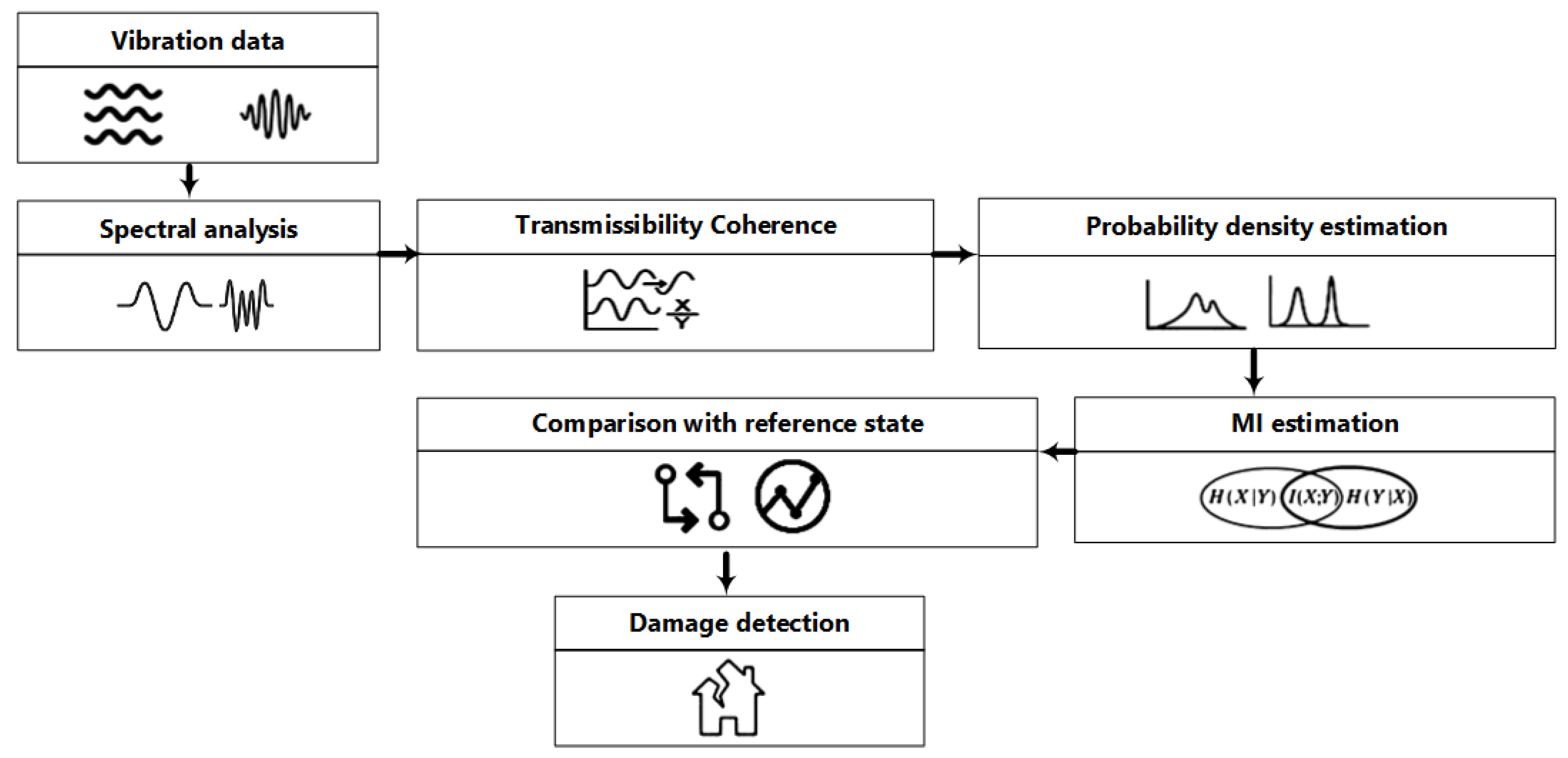
Figure 1 shows a flowchart for detecting damage using the proposed Mutual Infomation (MI)-based metric. We start with raw acceleration or displacement traces from each level of the structure. We then estimate their auto- and cross-power spectra and compute the transmissibility coherence, which measures the similarity of signals in the frequency domain. Next, using a two-dimensional histogram, we estimate the marginal and joint entropies and calculate the mutual information between the transmissibility coherences of the baseline (undamaged) and potentially damaged states. Finally, we compare MI value from an unknown to the average baseline MI to flag any significant deviations as potential damage events.

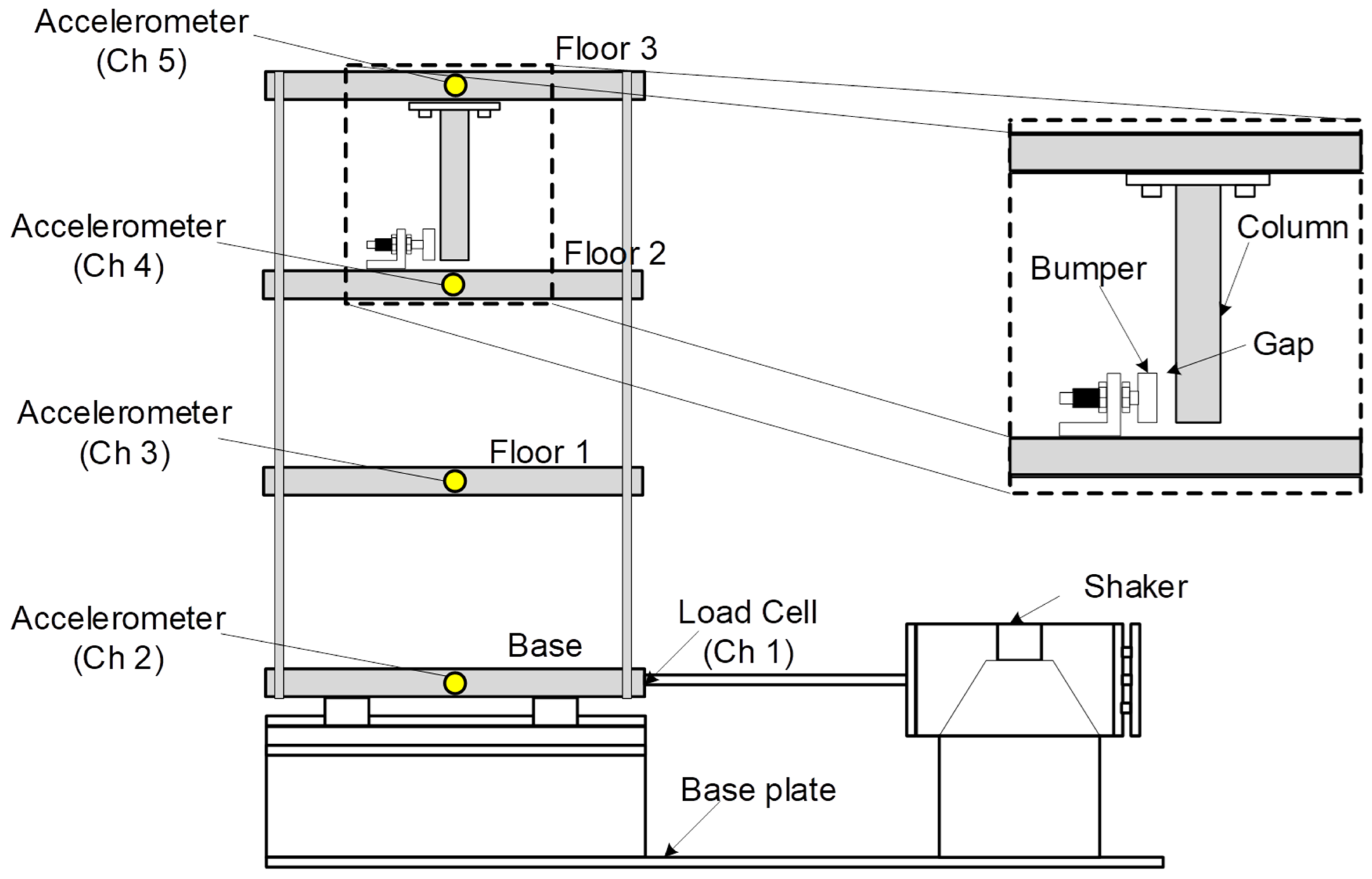
The method described in the flowchart is applied to a standard data set containing experimental data from a three-story aluminum frame structure. The results suggest that the proposed metric is a more sensitive damage indicator than two existing damage indices derived from transmissibility coherence $\left(TC\right)$ for both linear and nonlinear damage states.

The remainder of this paper is organized as follows. Section 2 provides an overview of transmissibility coherence and discusses existing damage indices derived from it. Section 3 introduces the concept of mutual information as a measure of similarity, which can be seen as an extension of the concept of correlation. Section 4 describes the proposed damage detection approach. Section 5 presents an application using a standard dataset containing experimental data from a three-story aluminum frame structure and compares the results from the proposed approach to two existing damage indices derived from the transmissibility coherence. Section 6 presents a discussion, and Section 7 concludes this paper.

2. Damage Detection Using Transmissibility Coherence

Measuring input excitation to actual civil engineering structures is notoriously difficult, if not impossible. This difficulty has motivated the development of “output-only” system identification methods that are based only on the response of the structure. The extraction of modal parameters under ambient/operational loading is known as operational modal analysis [22], and it has several variants that operate in the time, frequency, or wavelet domains [23,24,25]. Although the input excitation is not measured in operational modal analysis, certain assumptions (e.g., stationary, uncorrelated, and white noise with uniform spatial distribution) are made regarding the nature of the ambient or operational excitations. Research in wind- and human-induced load modeling [26,27,28,29,30,31] has raised questions about the validity of these assumptions. Transmissibility-based operational modal analysis [32] is an appealing way to reduce the effect of colored excitation on the estimated modal quantities. Transmissibility coherence, defined as the magnitude-squared coherence between a pair of response signals, has shown some promise as a damage-sensitive feature when used with data from numerical and experimental simulations of a simple shear frame [33]. A loss of transmissibility coherence can indicate damage. Zhou et al. [33] define two damage indices based on the transmissibility coherence and show that both indices can successfully detect nonlinear behavior induced in an initially linear system. However, these indices are not sensitive to mass or stiffness changes when the structure remains linear.

Following Zhou et al. [33], transmissibility coherence and related quantities are calculated as follows. Suppose that a harmonic force is applied at a given point l in a multi-degree-of-freedom system, and $x_i\left(t\right)$ and $x_j\left(t\right)$ are the measured responses at point i and a reference point j, respectively. The transmissibility between point i and reference point j is defined as follows:

$$T\left(i,j\right)={\displaystyle \frac{X_i\left(\omega \right)}{X_j\left(\omega \right)}},$$

(1)

where $X_i\left(\omega \right)$ and $X_j\left(\omega \right)$ are the complex amplitudes of the system responses, and $\omega$ is the frequency. Transmissibility can also be expressed in terms of the frequency response function $\left(H\right)$ as follows:

$$T\left(i,j\right)={\displaystyle \frac{{\displaystyle \frac{X_i\left(\omega \right)}{F_l\left(\omega \right)}}}{{\displaystyle \frac{X_j\left(\omega \right)}{F_l\left(\omega \right)}}}}={\displaystyle \frac{H_{il}\left(\omega \right)}{H_{jl}\left(\omega \right)}}.$$

(2)

As this definition requires knowledge of the excitation, a method to estimate transmissibility directly from two responses is desired. This leads to the concept of transmissibility coherence, which measures the similarity between two responses. Transmissibility coherence is computed as follows:

$$T{C}_{ij}\left(\omega \right)={\displaystyle \frac{|S_{i,j}{\left(\omega \right)|}^2}{S_{i,i}\left(\omega \right)S_{j,j}\left(\omega \right)}},$$

(3)

where $S_{i,i}\left(\omega \right)$ and $S_{j,j}\left(\omega \right)$ are the auto-spectrum of $x_i\left(t\right)$ and $x_j\left(t\right)$, respectively, and $S_{i,j}\left(\omega \right)$ is the cross-spectrum.

Transmissibility coherence can be used as a damage indicator based on the premise that damage induces a loss of coherence compared to the undamaged state. Specifically, Zhou et al. [33] define two damage indices based on transmissibility coherence. The first index, called Accumulation of Transmissibility Coherence (ATC) is defined as

$$ATC(i,j)={\int }_{f_{min}}^{f_{max}}T{C}_{ij}\left(f\right)df,$$

(4)

where $f_{min}$ and $f_{max}$ define the frequency interval of interest. A similar metric was previously defined by Rizos et al. [34]. The second index is called Transmissibility Modal Assurance Criterion (TMAC) and is calculated using the Modal Assurance Criterion [35] between the transmissibility coherence in the undamaged and damaged states of the structure, each expressed as a column vector in the frequency domain. $TMAC$ is given by the equation

$$TMAC(i,j)={\displaystyle \frac{{\left|d_{ij}^T{u}_{ij}\right|}^2}{\left(d_{ij}^T{d}_{ij}\right)\left(u_{ij}^T{u}_{ij}\right)}},$$

(5)

where $u_{ij}$ is the transmissibility coherence $T{C}_{ij}$ at the reference (undamaged) state, and $d_{ij}$ is that of the new, potentially damaged state. Statistically, $TMAC(i,j)$ is the square of the Pearson’s correlation coefficient between vectors $u_{ij}$ and $d_{ij}$ and as such is a number between 0 and 1, where 0 indicates that the two signals are uncorrelated, and 1 indicates that one of the signals can be written as a linear function of the other.

Damage detection using transmissibility coherence and metrics derived from it is an active area of research. Various damage metrics comparing the baseline transmissibility to that of a potentially damaged state have been proposed so far. The majority of these formulations can be grouped by their method of comparison into difference-based (e.g., [36,37,38]) and correlation/coherence-based approaches (e.g., [39,40]). Sampaio and Maia [41] define a new indicator for damage detection and relative damage quantification by examining the correlation between pairs of operational deflected shapes at the same frequency.

According to Meggitt and McGee [42], the appeal of the transmissibility concept, when properly defined, lies in its ability to describe the dynamics of a portion of a structure independent of the rest of the structure. This property, called sub-structural invariance, makes it possible not only to detect but also to locate damage in complex structures, provided that the transmissibility is defined between a set of internal and interface degrees of freedom. In practice, however, localization of damage is more challenging than detection. While the integral of the transmissibility contributions along the frequency axis—captured by the Accumulated Transmissibility Coherence (ATC) equation—can be used for damage detection, it is not necessarily suitable for locating damage. The difference between the transmissibility of baseline and damaged states tends to be large near modal frequencies, so any errors in the predicted damage locations accumulate and may mask the true location of damage for frequencies higher than the first modal frequency.

To circumvent this problem, Sampaio [43] proposed a normalization scheme based on counting the number of times the transmissibility difference is maximized at each potential damage location. A similar technique, which uses the transmissibility of several neighboring sensors, has been experimentally verified with data from static and fatigue tests of a full-scale wind-turbine blade [44].

3. Mutual Information

A fundamental SHM axiom is that damage increases the complexity of the system [45]. Shannon’s entropy [46] is a natural choice as a measure of complexity. The entropy H of a random variable X is given by the expected value of $-logp\left(x\right)$, where p describes the probability distribution (mass or density function). Joint and conditional entropy of two or more random variables are defined analogously, using the joint and conditional probability distributions, respectively. Mutual information $\left(I\right)$ between X and Y quantifies the average amount of information shared by X and Y and is defined in terms of joint and marginal entropies as follows:

$$I(X;Y)=H\left(X\right)+H\left(Y\right)-H(X,Y),$$

(6)

where $H\left(X\right)$ and $H\left(Y\right)$ are marginal entropies of X and Y, respectively, and $H(X,Y)$ is their joint entropy.

Mutual information $I(X;Y)$ can also be interpreted as the Kullback–Leibler divergence [15] between the joint distribution $p(x,y)$ and the product of the marginal distributions $p\left(x\right)p\left(y\right)$. Thus, it characterizes the deviation from independence. That is $I(X;Y)=0$ if and only if X and Y are independent random variables.

Figure 2 shows a Venn-like diagram, showing the relationship between entropy and mutual information of two random variables X and Y. Marginal entropies of X and Y are represented by the areas enclosed by the red and blue ellipses, respectively. The joint entropy $H(X,Y)$ is represented by the union of the two ellipses.

While mutual information is not the only similarity metric that can measure the strength of nonlinear relationships, it offers the following advantages [47]: Compared to the copula-based alternatives such as Kendall’s $\tau$ and Spearman’s $\rho$, which measure monotonic relationships, mutual information captures all types of nonlinear dependencies. As opposed to the Hilbert–Schmidt Independence Criterion, mutual information is invariant under scaling and other invertible transformations, which is important in signal-processing applications. Compared to distance correlation and the maximal information coefficient, mutual information has lower computational complexity, making it suitable for the analysis of large datasets.

Mutual information between two discrete random variables X and Y is defined as follows:

$$I(X;Y)=\sum _x\sum _{y}p(x,y)log\left({\displaystyle \frac{p(x,y)}{p\left(x\right)p\left(y\right)}}\right),$$

(7)

where $p(x,y)$ is the joint probability mass function and $p\left(x\right)$ and $p\left(y\right)$ are the marginal probability mass functions of X and Y, respectively. The logarithm can be evaluated using any base. Mutual information between continuous random variables X and Y is defined similarly, replacing the sums with integrals and replacing the probability mass functions with probability density functions.

In practice, the joint and marginal probability distributions required to compute the mutual information are unknown, and they need to be estimated from the observed data using a nonparametric method. A detailed description of multivariate density estimation methods can be found in [48].

As opposed to the correlation coefficient R, which measures the strength of linear association between a pair of measurements, mutual information measures the strength of functional dependence between them. In other words, it measures the amount by which the knowledge of one quantity decreases the uncertainty about the other. The $R^2$ value is commonly used as a measure of explanatory power in bivariate regression and is termed the coefficient of determination when used in this context. When the MI score is normalized to the $[0,1]$ interval, the resulting normalized MI score becomes comparable to $R^2$ in terms of the values it can take: a score of 1 indicates complete dependence, and a score of 0 indicates independence.

To demonstrate the robustness of MI scores compared to $R^2$, Figure 3 shows four scatterplots representing four types of relationships: perfect linear (a), linear with noise (b), linear with outliers (c), and nonlinear (d). Figure 3b shows that $R^2$ is more sensitive to noise than MI. The drastic reduction in $R^2$ with a small number of outliers is apparent in Figure 3c. The MI score in the nonlinear case (Figure 3d) remains high, indicating strong dependence between the two quantities. As $R^2$ measures only linear associations, it does not detect the nonlinear, yet strong, dependence depicted in Figure 3d.

4. Proposed Approach

In this section, we use the concept of mutual information to infer changes in the vibration behavior of structures. Such changes are often characterized as structural damage. Figure 1 shows a flowchart for detecting damage using the proposed MI-based metric. The proposed method can be considered an extension of the Transmissibility Modal Assurance Criterion (TMAC), where the similarity between two processes is measured in terms of the information shared between them. Mutual information is an elegant statistic that captures all types of dependence, as opposed to the correlation coefficient which only measures linear dependence.

The main ingredient of the proposed approach is a set of vibration signals measured at different points on the structure. These signals can be acquired using either contactbased sensors, such as accelerometers and strain gauges, or non-contact methods, such as vision-based techniques that extract displacement data from video recordings. Treating the response quantities as realizations of random variables, we estimate the information shared between response quantities and use its deviation from a reference (undamaged) state as a damage indicator.

Given a pair of response signals $(u_i,u_j)$ measured at locations i and j, respectively, in the reference (undamaged) state of the structure, and a pair of response signals $(d_i,d_j)$ measured at the same locations in a new (potentially damaged) state, the mutual information score $MI(i,j)$ between the two states is calculated as follows: First, we estimate the autoand cross-power spectra of $u_i$ and $u_j$, and normalize the cross-spectra using Equation (3). Call the resulting vector $u_{ij}$. Repeat the same using $d_i$ and $d_j$ from the new state. Call the resulting vector $d_{ij}$. Next, we estimate the joint and marginal probability mass functions of $u_{ij}$ and $d_{ij}$ empirically, using a two-dimensional histogram. Finally, we determine the mutual information between $u_{ij}$ and $d_{ij}$ using Equation (7).

Changes in the $MI$ scores between a reference (undamaged) state and a new state can be used to infer changes in the dynamic properties of structures. The rationale is as follows: mutual information between two random variables is zero if and only if the two random variables are independent and thus do not share any information, and it is maximized when one of the random variables is a deterministic function of the other. When there is a change in the structure that affects the underlying relationship between response processes at different locations, that change will be reflected in the mutual information scores. The proposed approach is similar to the correlation-based methods where a decrease in correlation is interpreted as damage but goes beyond assessing the strength of linear associations.

As the maximum value of mutual information depends on the entropies of the random variables, interpretation of mutual information requires either comparison to a reference state or normalization using an upper bound. For example, mutual information can be normalized to the range [0,1] by dividing the raw MI score by the summation of the marginal entropies of the random variables. The normalized MI score has the following interpretation: 0 indicates independence, and 1 indicates existence of a deterministic, not necessarily linear, relationship. Although normalization of MI makes it easier to interpret, we use the raw MI scores for the following reasons: First, normalized MI might not be directly comparable across different damage states as the total entropy is not necessarily constant in different states. In addition, MI normalization often leads to biased estimates, and, as formally demonstrated by Mahmoudi and Jemielniak [49], the bias becomes more pronounced as the size of the data increases. Apart from the bias concerns, as the proposed method uses changes in MI scores between a reference state and a potentially damaged state as a damage indicator, normalization would unnecessarily increase the computational burden.

5. Example Application

Below, we show how the mutual information (MI)-based damage index compares with the two coherence-based metrics described in Section 2–namely, $ATC$ and $TMAC$–in detecting and quantifying damage in structures. We use a standard dataset produced by Los Alamos National Laboratory [50] for this purpose. The same dataset was used by Zhou et al. [33] to investigate the performance of $ATC$ and $TMAC$.

5.1. Vibration Data

Experimental data from a three-story aluminum frame structure equipped with an adjustable bumper and a suspended column was used. Figure 4 shows the experimental setup. Details about the experimental setup and damage states can be found in the report [51].

In this SHM testbed, the definition of the non-linear damage to be detected is ’crack’ formation in a suspended central column that occasionally hits an adjustable aluminum bumper (Figure 4). This mechanism simulates how a crack opens and closes; a crack-like nonlinear damage mode. When the crack and buffer gap stay open, the system behaves linearly. Impact events cause local yielding, joint slip, and clear nonlinear signatures in response. The operational and environmental variability is simulated in several ways. Thermal effects are simulated by using columns with reduced-thickness specimens to change their effective Young’s modulus. Live-load changes are simulated by adding weights at the base or on the first floor. Varying excitation levels (± drive voltage to the shaker) are simulated to mimic changing operational loads. Data acquisition limits reflect real-world challenges. Economic limitations allow for only one accelerometer per floor. They are mounted on the centerline without any formal optimal placement studies. There is no direct measurement of the input force, just a single base load cell, meaning we monitor output only. All channels are sampled at 320 Hz, and a dynamic range of ±4 g is set by the sensor and the limits of the A/D converter.

The dataset contains 170 sets of acceleration signals from 17 structural states, each state with 10 measurements.

Table 1. Description of structural states.

Label	Category	State	Description
1	0	Baseline	Baseline condition
2	I	State #2	1.2 kg mass at the base
3	I	State #3	1.2 kg mass on Floor 1
4	I	State #4	87.5% stiffness reduction in column 1BD
5	I	State #5	87.5% stiffness reduction in columns 1AD and 1BD
6	I	State #6	87.5% stiffness reduction in column 2BD
7	I	State #7	87.5% stiffness reduction in columns 2AD and 2BD
8	I	State #8	87.5% stiffness reduction in column 3BD
9	I	State #9	87.5% stiffness reduction in columns 3AD and 3BD
10	II	State #10	0.20 mm gap
11	II	State #11	0.15 mm gap
12	II	State #12	0.13 mm gap
13	II	State #13	0.10 mm gap
14	II	State #14	0.05 mm gap
15	III	State #15	0.20 mm gap and 1.2 kg mass at the base
16	III	State #16	0.20 mm gap and 1.2 kg mass on Floor 1
17	III	State #17	0.10 mm gap and 1.2 kg mass on Floor 1

describes these states and groups them into four categories. State #1, representing the baseline state (Category 0), is the reference state from which deviations will be considered in damage detection. Category I (State #2–#9) contains the linear damage states obtained by changing the stiffness of one or two columns or adding a mass to the base or the first floor. Category II (State #10–#14) contains the damage states where the damage is simulated by introducing nonlinear behavior via adjusting the gap. A small bumper (clearance gap) is situated between a suspended central column and an adjustable block. When the gap is small enough, the column intermittently hits the bumper, producing joint slip, bracket loosening, and local effects, yielding true nonlinear damage. Category III (State #15–#17) represents damage states obtained by simulating nonlinear behavior combined with a change in mass.

The dataset contains 10 sets of measurements from each state. Each acceleration signal contains 8192 time-domain samples with a sampling frequency of 320 Hz. To compare the performance of the proposed $MI$ index to $ATC$ and $TMAC$ we will use the same signals used in Zhou et al. [33], namely the acceleration signals from Channel 2 (base), Channel 3 (first floor), and Channel 5 (third floor).

5.2. Calculation of $ATC$, $TMAC$, and $MI$ Scores

$ATC$, $TMAC$, and $MI$ scores between Channel 2 and Channel 5 and those between Channel 3 and Channel 5 were computed as follows: To compute the auto- and cross-power spectra, Welch’s method [52] was used with a Hann window of 2096 time points and 50% overlap.

Welch’s method produces an estimate of the power spectral density of a signal by dividing the signal into overlapping segments of equal length, applying a window function to each segment, computing the periodogram of each windowed segment, and averaging the resulting periodograms. The window function acts to mitigate the spectral leakage resulting from analyzing a finite portion of the signal. However, since the window function tends to zero at the boundaries, data points near the boundaries have a smaller influence on the periodogram than those near the midpoint. To equalize the influence of each data point on the resulting PSD, segments are overlapped. The amount of overlap is often selected to be between 50–75%. Specifically, when the Hann window is used, 50% overlap is considered optimal, as it ensures equal contribution of each data point in the resulting PSD estimate [53]. The choice of window length determines the trade-off between the frequency resolution and the variance of the estimate. A shorter window leads to reduced spectral variance at the expense of frequency resolution. In this study, the window length was set to 2048 to achieve a good balance between spectral variance and frequency resolution. With a sampling frequency of 320 Hz, this window length corresponds to a frequency resolution of 0.156 Hz. Although the Dactron SpectraBOOK system [54] used in data acquisition has an operational frequency range from 0.1 Hz to 100 kHz, the analysis here is bounded by the sampling frequency of 320 Hz. The frequency resolution of 0.156 Hz is appropriate to analyze the vibration characteristics of the selected window length.

The transmissibility coherence between two channels $(i,j)$ was computed by normalizing the cross-power spectra using Equation (3). $ATC$ scores between Channel 2 and Channel 5 and those between Channel 3 and Channel 5 were calculated using Equation (4), between $f_{min}=$ 20 Hz and $f_{max}=$ 80 Hz. $TMAC$ scores were calculated using Equation (5), using the first measurement from State 1 as the reference signal. To calculate the $MI$ scores, joint and marginal probabilities were estimated using a 2D histogram, with 15 bins in each direction. The number of bins b was selected using the equation derived by Hacine-Gharbi et al. [55]:

$$b=\mathrm{round}\left({\displaystyle \frac{e}{6}}+{\displaystyle \frac{2}{3}}e+{\displaystyle \frac{1}{3}}\right),$$

(8)

where $\mathrm{round}\left(x\right)$ indicates the integer closest to x, and e is given by

$$e=\sqrt[3]{8+324n+12\sqrt{36n+729n^2}},$$

(9)

for a vector of length n. Hacine-Gharbi et al. [55] show that Equation (8) leads to a low bias in histogram-based estimation of entropy. Mutual information was then computed from the estimated probabilities using Equation (7).

5.3. Results

Because $ATC$, $TMAC$, and $MI$ scores do not measure the same quantity; we convert these scores to percent deviation scores to facilitate their comparison. To do this, we first compute a reference score for each metric by computing the average score from the 10 baseline measurements (State #1):

$$x_{ref}={\displaystyle \frac{1}{10}}\sum _{k=1}^{10}x\left(k\right),$$

(10)

where $x\left(k\right)$ is the score ($ATC$, $TMAC$, or $MI$) for the kth measurement. Next, the percent deviation of the kth measurement from the reference was calculated using

$$q_{\left(k\right)}={\displaystyle \frac{x\left(k\right)-x_{ref}}{x_{ref}}}\times 100,\mathrm{for}k=1,2,\dots ,170$$

(11)

Noting that $q\left(k\right)$ where $10(s-1)\le k\le 10s$ belong to State #s, percent deviations corresponding to each structural state were presented using a box plot. The bottom and top edges of each box indicate the lower and upper quartile, respectively, and the mark between the two edges is the median (50th percentile). The symbol ’o’ shows the outliers, and the whiskers extend to the lowest and highest values not considered outliers.

Figure 5a shows the percent deviation in $ATC(5,2)$ and Figure 5b shows the same for $ATC(5,3)$. Figure 6a and Figure 6b show the percent deviation in $TMAC(5,2)$ and $TMAC(5,3)$, respectively. Figure 7a and Figure 7b show the percent deviation in $MI(5,2)$ and $MI(5,3)$, respectively. These figures present a series of side-by-side box plots summarizing the distribution of the three metrics across all seventeen states. Each graphical element encodes the box outlines, showing the interquartile range for each state. The thick horizontal line inside each box marks the median value for that state. Whiskers extend to the most extreme non-outlier points, while any measurement beyond those bounds is plotted individually as an outlier dot. To highlight differences between groups of states, three vertical lines divide the 17 boxes into Category I (States #2–#9), Category II (States #10–#14), and Category III (States #15–#17).

Based on these figures, the following observations can be made:

• Category I (States #2–#9): $ATC$ and $TMAC$ show less than 0.5% deviation from the baseline. Thus, $ATC$ and $TMAC$ are not sensitive to changes in stiffness and mass when the structure remains linear. In contrast, $MI$ scores show a significant reduction compared to the reference state.
• Category II (States #10–#14): All three metrics show significant reductions from the baseline when nonlinearity is induced using the adjustable gap. $ATC$ appears to be the most sensitive, although the monotonous drop in $ATC$ as the adjustable gap is decreased is unexpected. However, $TMAC$ scores for State #10 show very high variability and an unexpectedly large drop in State #11, compared to the other states in the same category. In contrast, $MI$ scores for State #11 show high variability like $TMAC$ scores, although not as extreme.
• Category III (States #15–#17): In all three figures, State #15 and State #16 appear to be on the same level as State #10. These three states are the ones where the adjustable gap was set to its maximum value (0.20 mm). $ATC$ and $TMAC$ scores of these states are close to the baseline, suggesting that these states may not be identified as damaged. In contrast, $MI$ scores indicate a significant difference between these states and the baseline state.

The observed behavior is discussed in more detail in Section 6.1.

6. Discussion of Results

6.1. Qualitative Description of the Damage Detection Ability of the Three Metrics

A reduction in MI implies a reduction in the joint probability as estimated from a 2D histogram. This, in turn, implies the following: Imagine a scatter plot (SP1) showing the transmissibility coherence $T{C}_{ij}$ vector representing the mean baseline state on the x axis, and a $T{C}_{ij}$ vector from the baseline state is on the y axis. SP1 is expected to contain $N_f$ points, where $N_f$ is the length of the frequency vector. All of these points are expected to lie close to the line $y=x$. If we create a second scatter plot (SP2), this time using a $T{C}_{ij}$ vector from an unknown state on the y axis, the points on SP2 may or may not be close to the line represented by the equation $y=x$. We may observe the following three cases:

• Case 1: SP2 appears similar to SP1. All three metrics suggest that there is no damage.
• Case 2: SP2 contains $N_f$ points close to a line $y=ax+b,$ where $a\ne 1$. In this case, ATC and TMAC may fail to detect any change. The correlation coefficient is close to 1, even though the slope may be very different from that in SP1. On the other hand, MI will likely detect the change, as the points in SP1 and SP2 no longer occupy the same grids on the $(x,y)$ plane. The amount of change in MI depends on the number of points, the number of grids in the x and y directions, and how the number of points in each grid changes between SP1 and SP2.
• Case 3: SP2 is very different from SP1; the points in SP2 do not lie close to any particular line. In this case, both ATC and TMAC detect damage since the correlation coefficient has decreased. MI will also detect damage since a large portion of the $N_f$ points occupy different grids in SP1 and SP2.

A large decrease in MI accompanied by small changes in ATC and TMAC is consistent with the behavior described in Case 2. This suggests that the modal frequencies of the system have changed. As mass and stiffness changes lead to changes in modal frequencies, the observed behavior is indicative of Category 1 damages.

6.2. Statistical Significance

It was shown in Section 5 that all three metrics are able to differentiate the nonlinear damage states from the baseline state. In this section, we focus on the performance of the three metrics for the linear damage states (States #2–#9). Specifically, for each pair of damage states, we test the statistical significance of the difference between the population means of the damage metric corresponding to these states. We use nonparametric bootstrapping [56] to obtain the p-values, as bootstrapping does not require assuming an underlying probability distribution, as opposed to commonly used tests such as the two-sample t-test. The p-value of a test indicates the probability of observing results as extreme as or more extreme than the results observed in the study, if the null hypothesis holds true. The null hypothesis is that the population mean of the damage metric is the same in the two states being compared. A p-value exceeding a preselected threshold (e.g., 0.01 or 0.05) can be interpreted as a lack of evidence to reject the null hypothesis, indicating a lack of statistical significance. In the context of the damage detection problem addressed in this paper, a large p-value indicates that the damage metric obtained for one damage state is not significantly different from the other damage state, thus indicating that the two damage states cannot be reliably distinguished using the damage metric selected.

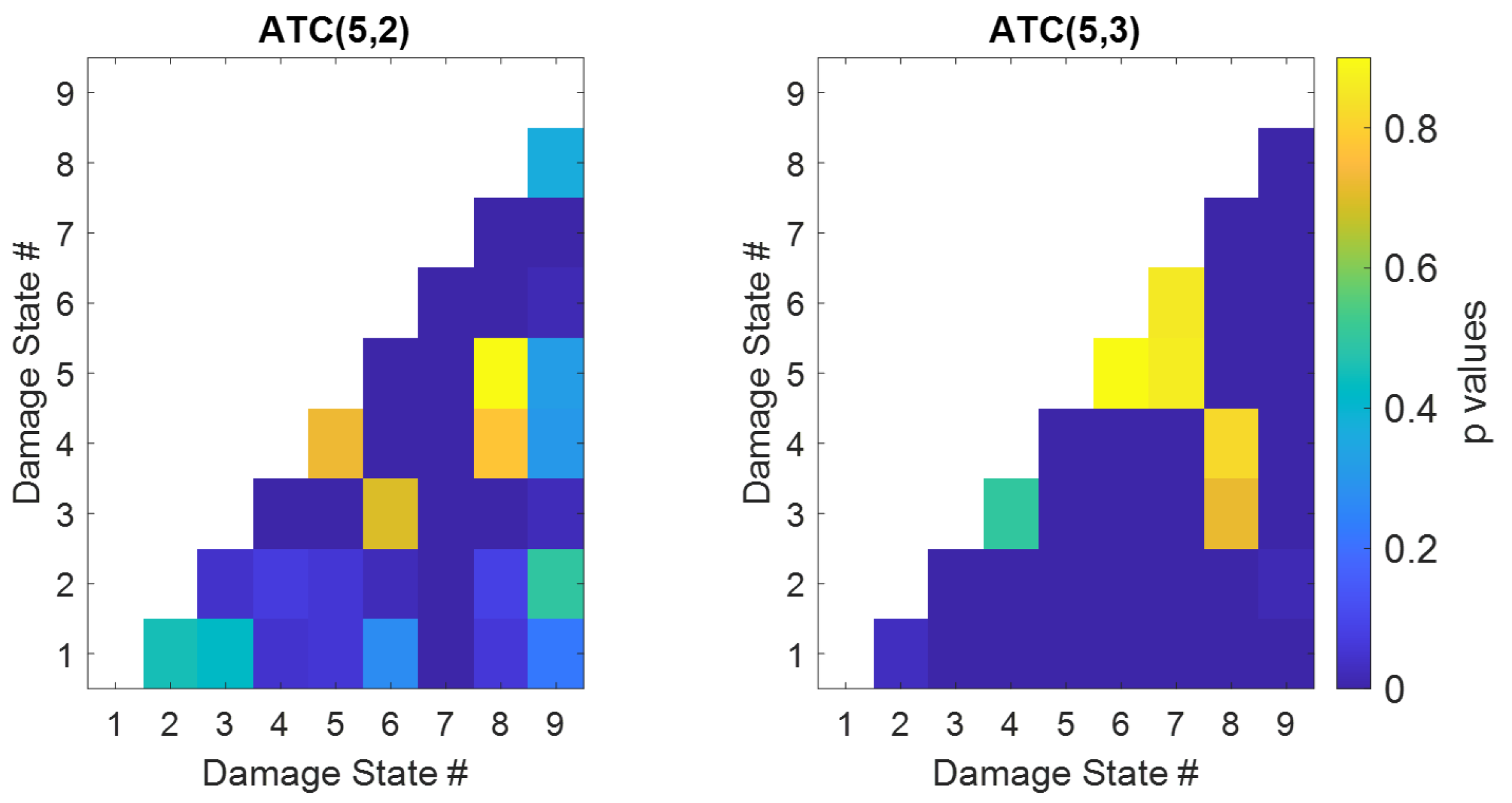
Bootstrapping was performed using 10,000 repetitions, resulting in a $9\times 9$ matrix of p-values. The $(i,j)$th entry of this matrix quantifies the probability that the observed difference between damage states i and j could have occurred by random chance, if in fact there was no difference in the average damage metric associated with the two states. Considering that the matrix of p-values is symmetric, the likelihood of damage can be assessed by setting i or j to the baseline (undamaged) state.

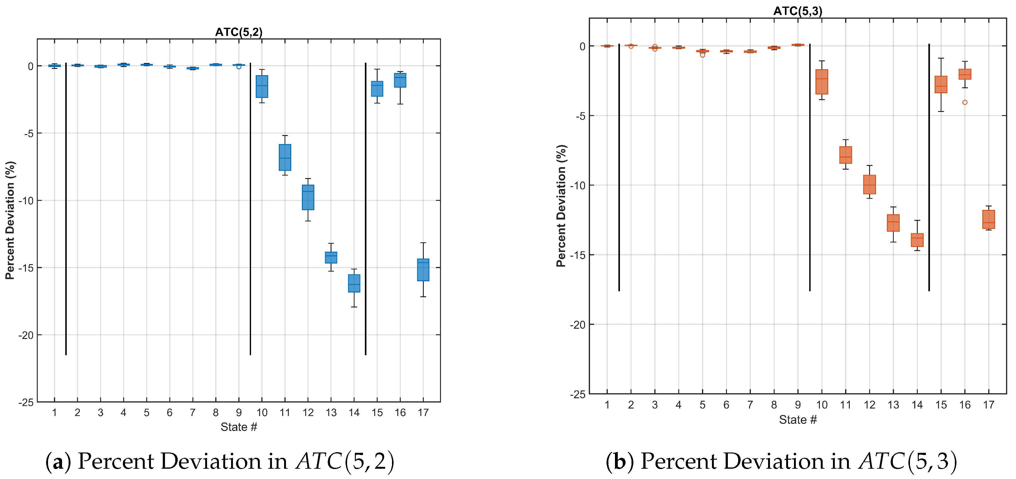
Figure 8 shows the results of significance testing for the quantities ATC(5,2) and ATC(5,3). In each of the two windows, the bottom row indicates the p-values in distinguishing damage states 2 through 9 from the baseline (undamaged) state. The largest p-values in the bottom row of the ATC(5,2) matrix is 0.436, and that in ATC(5,3) is 0.028. Thus, it can be concluded that the observed differences in the ATC metric between the damaged and undamaged states are not statistically significant at the 0.01 level, while the ATC(5,3) case is statistically significant at the 0.05 level. The p-values above the bottom line have values exceeding 0.8, indicating that the ATC metric is unable to differentiate between different damage states.

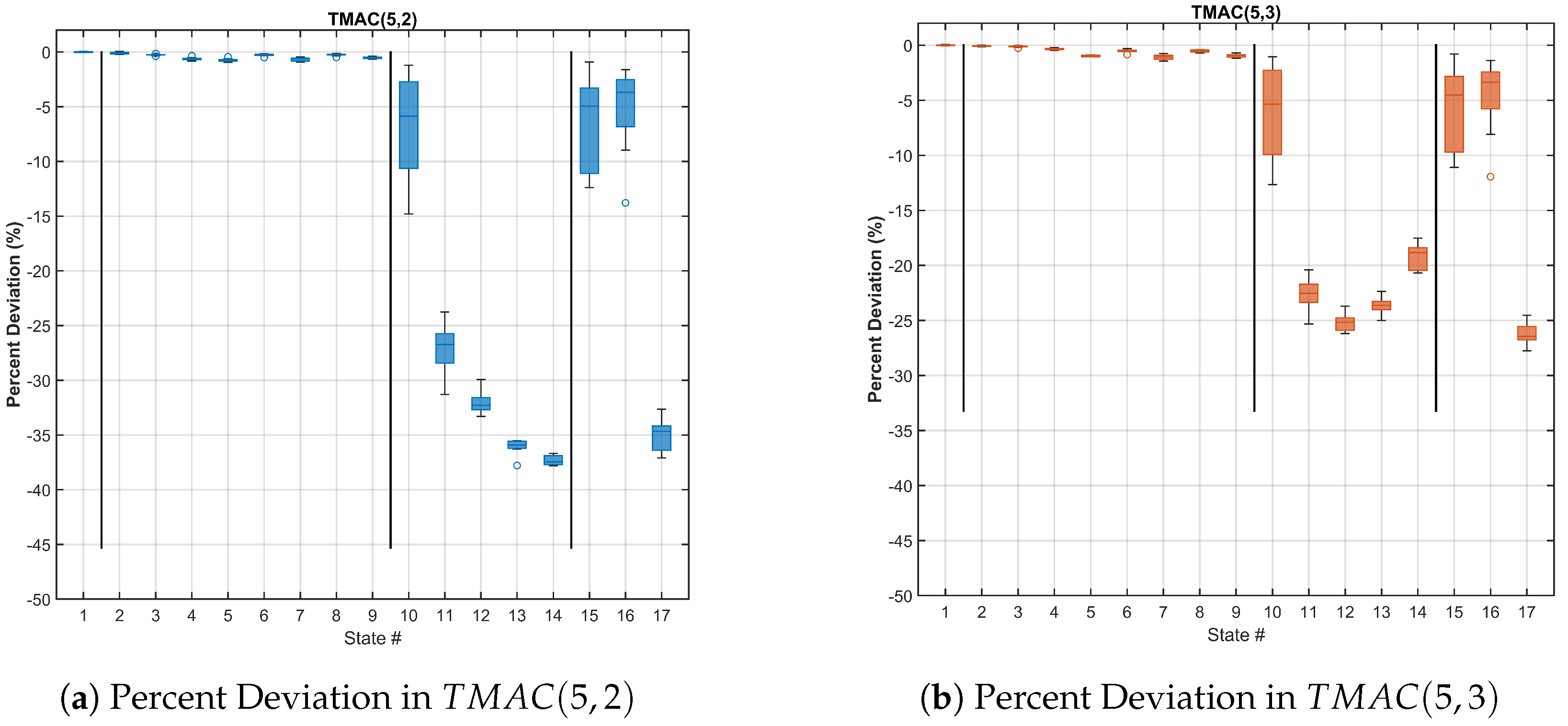
Figure 9 shows the results of significance testing for the quantities TMAC(5,2) and TMAC(5,3). The largest p-value in the bottom row of both TMAC(5,2) and TMAC(5,3) is less than 0.01, indicating that the observed differences between the TMAC values in each damage state and those in the undamaged state are statistically significant at the 0.01 level. As in the TMAC case, the p-values above the bottom line have values exceeding 0.8, indicating that the TMAC metric is unable to differentiate between two damage states.

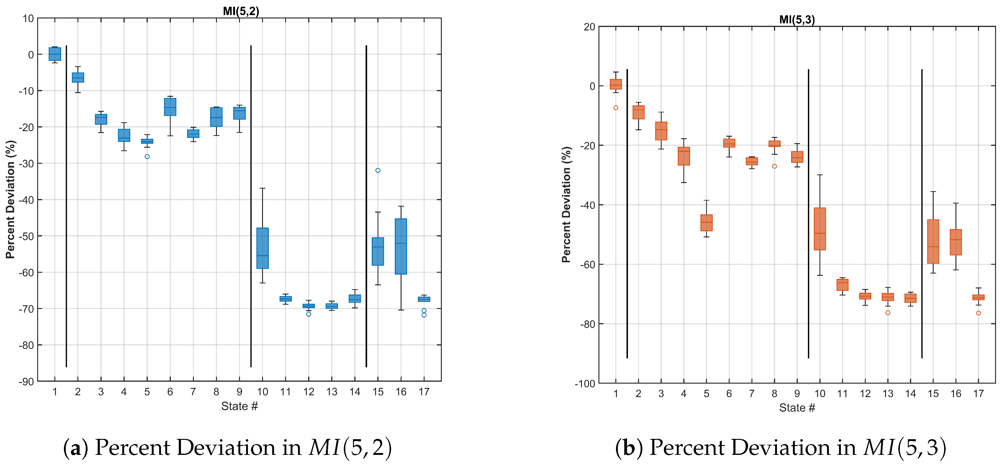
Figure 10 shows the p-values for the quantities MI(5,2) and MI(5,3). The largest p-value in the bottom row of both MI(5,2) and MI(5,3) is less than 0.01, indicating that the observed differences between the MI values in each damage state and those in the undamaged state are statistically significant at the 0.01 level. The p-values above the bottom line, in general, are smaller than both the ATC and TMAC values, showing that the MI metric has a better ability to distinguish between different damage states, compared to the other two metrics, although the MI metric is unable to differentiate certain pairs of damage states.

To investigate the effect of noise on the p-values, the bootstrap analysis described above was repeated with noisy acceleration signals. Zero-mean Gaussian white noise was added to the acceleration signals at levels corresponding to 30 dB, 25 dB, and 20 dB signal-tonoise ratios. Even at the 20 dB level, p-values did not show noticeable deviations from the values depicted above. While we cannot fully explain this behavior, we offer the following observations. First, the presence of noise mostly affects the high frequency range, leaving the transmissibility coherences in the low frequency range essentially unchanged. For the ATC metric, using an upper limit of 80 Hz in the integration greatly reduces the effect of noise. For the TMAC metric, which measures the correlation between two transmissibility coherence vectors, many of the values are close to 1 regardless of the presence of noise; any noise-related changes in TMAC are not large enough to modify the significance testing results. That is, statistically significant observations in the noise-free case remain statistically significant after the addition of noise. We note that correlation is generally considered a noise-sensitive metric. However, the effect of noise added to the acceleration signals is largely diminished during the transmissibility coherence calculations. If we were to artificially introduce changes to the transmissibility coherences instead of adding white noise in the time domain, the TMAC values would decrease. The lack of sensitivity of the MI metric is expected not only due to the lack of large differences in the transmissibility coherences compared to the noise-free case, as in the TMAC case, but also the intrinsic robustness of the mutual information measure to noise.

6.3. Computational Complexity

The computational complexity of mutual information estimation using the histogram method is of the order $\mathcal{O}(N_f+b^2)$, where $N_f$ is the length of the frequency vector used in transmissibility coherence calculations, and b is the number of bins used in marginal entropy calculations. Note that since $b^2$ must be smaller than $N_f$ for the binning process to be meaningful, the computational complexity can be written as $\mathcal{O}\left(N_f\right)$. The Pearson’s correlation coefficient has the same level of complexity. As a reference, the Discrete Fourier Transform has a complexity of $\mathcal{O}(NlogN)$, where N is the number of samples in the time domain. Thus, mutual information is suitable for real-time applications.

7. Conclusions

A new damage metric based on the concept of mutual information was proposed, and its performance was compared to two existing damage metrics that use output-only vibration data. The major advantage of mutual information over correlation as a similarity measure is that mutual information measures the amount of information shared between a pair of measurements while correlation measures only the strength of linear associations. In addition, because marginal and joint probabilities are estimated directly from the data as part of mutual information estimation, assumptions regarding the underlying distribution of the data (e.g., Gaussian) are not needed.

A standard data test was used to demonstrate the method. The dataset contains acceleration time series measured at each level, collected under 17 different structural states representing undamaged, linear damage, and nonlinear damage conditions. The linear damage states represent the case where the structure remains linear, but with modified stiffness and/or mass. The nonlinear damage is simulated using an adjustable gap to mimic the opening and closing of fatigue cracks under load reversals. The statistical significance of the proposed method was assessed using nonparametric bootstrapping.

Damage detection results obtained using the proposed damage metric were compared to those obtained using ATC and TMAC. The following conclusions can be drawn from the results of this study: (1) the MI-based damage metric proposed in this study is able to detect the existence of damage in all structural states of the model frame; (2) compared to ATC and TMAC, the proposed metric has a better ability to distinguish linear damage states from the baseline state; (3) the proposed metric shows some potential in differentiating between different damage states, although the observed differences are not statistically significant for all pairs of damage states. In terms of noise sensitivity, addition of zeromean Gaussian white noise up to a signal-to-noise ratio of 20 dB does not appear to cause noticeable differences in the p-values in any of the three metrics.

An important limitation of the method described in this study, which is shared by a large class of existing output-only damage detection methods, is that it requires data from the baseline condition of the structure, which may not be available. Further, because of the inherent assumption of stationarity in evaluating transmissibility coherences, abrupt damages that cause transient changes in the vibration characteristics, such as those induced by wind or earthquake, cannot be reliably detected. Although the method used in this paper, in its current form, is not intended for real-time SHM applications, it can be extended to such applications by using wavelet-based transmissibility instead of its Fourier-based counterpart. The computational complexity of such an approach will be governed by the transmissibility calculations, rather than that of the mutual information calculations.

In addition to extending this approach to the nonstationary case, future research will focus on the problem of selecting the locations where the responses are to be measured and the interpretation of the damage indices. While simulations using a finite element model of the structure can provide significant insight into how different damage scenarios affect a particular damage index, the inverse problem of characterizing damage and predicting its location based solely on the damage index remains a challenge. Extension of the bivariate mutual information to the multivariate case or conditioning the mutual information between two channels on additional channels can be very helpful in tracking changes in the dynamic properties of complex structures. Time-delayed mutual information computed using a time-delayed version of one of the signals can be used to infer the direction of nonlinear interactions between the responses collected at different channels, which can indicate the type and location of the damage.