Article

Power–Cadence Relationships in Cycling: Building Models from a Limited Number of Data Points

by
David M. Rouffet
1,2,*,
Briar L. Rudsits
3,4,
Michael W. Daniels
5,
Temi Ariyo
1 and
Christophe A. Hautier
2
1
Department of Health and Sport Sciences, University of Louisville, Louisville, KY 40208, USA
2
Laboratoire Inter-Universitaire de Biologie de la Motricité (UR 7424), Université Claude Bernard Lyon 1, 69100 Villeurbanne, France
3
UK Sports Institute, Manchester M11 3BS, UK
4
Manchester Institute of Health & Performance, Manchester M11 3BS, UK
5
Department of Bioinformatics & Biostatistics, University of Louisville, Louisville, KY 40208, USA
*
Author to whom correspondence should be addressed.
Signals 2025, 6(3), 32; https://doi.org/10.3390/signals6030032
Submission received: 10 June 2025 / Revised: 3 July 2025 / Accepted: 8 July 2025 / Published: 10 July 2025

Abstract

Accurate modeling of the power–cadence relationship is essential for assessing maximal anaerobic power (Pmax) of the lower limbs. Experimental data points from Force–Velocity tests during cycling do not always reflect the maximal and cadence-specific power individuals can produce. The quality of the models and the accuracy of Pmax estimation is potentially compromised by the inclusion of non-maximal data points. This study evaluated a novel residual-based filtering method that selects five strategically located, maximal data points to improve model fit and Pmax prediction. Twenty-three recreationally active male participants (age: 26 ± 5 years; height: 178 ± 5 cm; body mass: 73 ± 11 kg) completed a Force–Velocity test consisting of multiple maximal cycling efforts on a stationary ergometer. Power and cadence data were used to generate third-order polynomial models: from all data points (High Number, HN), from the highest power value in each 5-RPM interval (Moderate Number, MN), and from five selected data points (Low Number, LN). The LN model yielded the best goodness of fit (R2 = 0.995 ± 0.008; SEE = 29 ± 15 W), the most accurate estimates of experimentally measured peak power (mean absolute percentage error = 1.45%), and the highest Pmax values (1220 ± 168 W). Selecting a limited number of maximal data points improves the modeling of individual power–cadence relationships and Pmax assessment.

Graphical Abstract

1. Introduction

The Force–Velocity test performed on a stationary cycle ergometer is a well-established method used by researchers and practitioners to assess the neuromuscular function of the lower limbs. The experimental data collected during this test are often analyzed to estimate maximal anaerobic power [1,2,3,4,5], a physiological parameter of interest for evaluating athletic performance [6,7,8,9,10,11,12,13,14,15], fatigue [16,17,18,19], or age-related changes in neuromuscular function [20,21].
Since the early development of this testing approach, various protocols and ergometer designs have been proposed, each of which can influence the quality and characteristics of the data collected. A central objective of any Force–Velocity testing protocol is to generate data that reflects the participant’s true maximal force and power output across a wide range of cadences [5]. However, fatigue and suboptimal execution of the pedaling task can lead to the collection of data points that do not reflect true maximal values. To mitigate this issue, most protocols limit the duration of each sprint to approximately 6–7 s, restrict the number of maximal efforts (typically 3 to 6), and incorporate 3–5 min of rest between efforts. Despite these precautions, it remains common to observe substantial variability in power output at similar cadences across maximal efforts and across pedal cycles [5,7,22]. As previously demonstrated by our group, such variability is associated with differences in lower limb muscle activation levels [5]. To improve the consistency of maximal power expression during testing, some researchers have recommended the use of familiarization sessions in which participants repeat the protocol across multiple days [21,23,24], for a better assessment of their maximal power generating capacities. This somehow mirrors the standard practice used in neuromuscular assessments involving maximal voluntary contractions, where several attempts are made to capture a true maximum. Similarly, collecting multiple data points at the same cadence during a single testing session increases the likelihood of capturing cadence-specific maximal power outputs. However, applying this principle during a single force–velocity test must be done cautiously to avoid excessive fatigue, which may arise from accumulating too many maximal efforts or an overly long total duration of the Force–Velocity testing.
In addition to variability in testing protocols, notable differences exist in how experimental data collected during Force–Velocity testing in cycling are processed. These differences pertain to three main aspects. First, researchers have modeled different types of relationships. Some have estimated Pmax by extrapolating the y- and x-intercepts of the force or torque vs. cadence relationships [4,8,9,15,16,17,25,26,27,28], while others have relied on modeling the power vs. cadence relationship to estimate Pmax more directly [1,5,7,10,11,12,13,15,21,22,29,30,31,32]. Second, various modeling approaches have been employed to characterize the power–cadence relationship. A commonly used method assumes that this relationship follows a symmetric parabola and applies second-order polynomial regression [1,4,7,8,9,13,15,16,17,18,25,26,27,28,29,30,32,33,34,35,36,37,38]. In contrast, an alternative approach recognizes that the shape of the power–cadence curve may differ between individuals and deviate from symmetry, thus requiring a third-order polynomial model [5,10,11,12,21,22,39]. The superiority of this latter approach has been demonstrated by two different studies [5,10]. Third, strategies for selecting and aggregating data points vary substantially. These include processing each maximal effort independently [15,16,21,22], aggregating all data across multiple efforts [1,4,5,6,7,9,11,12,13,26,27,28,29,32,33,34,39], or selecting a single maximal data point per cadence or cadence interval [3,5,10,11,12,15,18,37,38]. In this regard, we previously proposed a residual-based filtering method in which only the data point with the highest value in each 5-RPM cadence bin was retained [5]. While this method improves the likelihood of capturing truly maximal efforts, it loses validity when cadence bins include only one or no data points, thereby increasing the risk of including submaximal efforts. When such points are incorporated, the resulting power–cadence curve may be artificially lowered or flattened, and ultimately underestimating Pmax. This issue can often be identified through visual inspection of power–cadence models overlaid with experimental data points, where truly maximal and cadence-specific data points appear poorly fitted [6,7,21,22,28,34,38,39].
To improve the selection of a limited number of truly maximal data points, it is essential to consider the mathematical characteristics of the power–cadence relationship and the third-order polynomial regression. The accuracy of the model depends on using maximal data points strategically distributed across three cadence regions: low cadences (influencing the initial slope), cadences near the apex (shaping the curvature), and high cadences (defining the descending limb). By varying external resistance across efforts, it is feasible to generate data points spanning the lower, middle, and upper ends of the cadence spectrum [5,7,11,12,22]. Therefore, a small set of strategically placed data points may be sufficient for accurate curve fitting, thereby reducing the total number of efforts required and minimizing participant fatigue.
The primary objective of this study was to develop and evaluate a new filtering method for selecting a limited number of data points that best represent an individual’s maximal power-generating capacity across key cadence ranges, with the goal of improving the accuracy of individual-specific power–cadence profiling. We hypothesized that a third-order polynomial model based on five strategically selected maximal data points; one drawn from low cadences, three drawn from medium cadences (around the apex of the curve), and one drawn from high cadences; would provide estimates of Pmax comparable to, or better than, those obtained from models using larger numbers of data points.
To test this hypothesis, we analyzed data from 23 participants. We compared three modeling approaches: (i) a High-Number (HN) model based on all available data, (ii) a Moderate-Number (MN) model based on our previously proposed 5-RPM bin method, and (iii) a Low-Number (LN) model based on five data points selected from key regions of the curve using a residual-based filtering strategy. We evaluated each model in terms of curve goodness of fit, Pmax estimates, and how well each model predicted experimentally measured peak power (Ppeak) at the corresponding cadence.

2. Materials and Methods

Twenty-three males (age: 26 ± 5 years; height: 178 ± 5 cm; body mass: 73 ± 11 kg), all of whom regularly engaged in physical activity through various recreational activities (e.g., endurance running, sprinting, basketball, road cycling, martial arts, resistance training, rowing, rugby union, soccer), volunteered to participate. Informed consent was obtained from each participant, and the study was conducted in accordance with the principles of the Declaration of Helsinki. The study was performed as part of the corresponding author’s PhD research [40].
All participants were tested on a stationary cycle ergometer (Monark 818E, Stockholm, Sweden) equipped with a strain gauge (200 N, bandwidth 500 Hz) to measure frictional force, and an optical encoder (1969.2 points/m of displacement or 11,815 points/revolution) to measure flywheel displacement [22]. Friction force and displacement signals were sampled at 200 Hz and recorded via a 12-bit analog-to-digital interface card (DAS-8, 12-bit, Keithley Metrabyte, Taunton, MA, USA). Flywheel velocity and acceleration were calculated as the first and second derivatives of displacement, respectively. External torque was computed as the sum of frictional torque (measured via the strain gauge) and the torque required to accelerate the flywheel [41,42]. The flywheel’s moment of inertia (I) was calculated as 0.927 kg·m2 (m = 22.5 kg) using the free deceleration method previously described [41]. The strain gauge was calibrated, and the inertia of the flywheel was verified both before and after data collection.
All participants completed a standardized warm-up protocol followed by a 5-min rest period. They then performed four 6-s maximal cycling sprints, each separated by 5 min of rest. All sprints were initiated from a stationary start. Three sprints were performed against the combined resistance of the flywheel’s inertia and frictional belt forces set at 0.3, 0.7, or 1.1 N·kg−1 of body mass. One sprint was performed against the inertia of the flywheel only. The order of sprints was randomized for each participant. Prior to each sprint, participants were instructed to generate maximal acceleration during every pedal cycle while remaining seated and keeping their hands on the drops of the handlebars. Strong verbal encouragement was provided throughout each sprint.
Average torque and cadence were calculated over the downstroke phase of each pedal cycle, and average power was derived from these values [42]. Power–cadence pairs from all maximal efforts were pooled for each participant to construct their individual power–cadence relationships [5]. To model the individual power–cadence relationship, third-order polynomial regression was applied to the data points considered. The general form of the equation used is:
y(x) = ax + bx2 + cx3
where y is power (W), x is cadence (RPM), and a, b, and c are coefficients that define the shape of the curve.
As a first step, we examined the distribution of data points across cadences (Figure 1).
In addition to the uneven distribution of experimental data points across cadences (Figure 1a), the cadence-specific power levels varied considerably across pedal cycles and maximal efforts. While some data points appeared to reflect true maximal power output at a given cadence, others were clearly submaximal (Figure 2).
Considering this, we applied two residual-based filtering strategies to select subsets of data for modeling the power–cadence relationship of each participant. These were compared against a model built from the complete dataset. All models were generated using third-order polynomial regression with the intercept fixed at zero [5,11,12], because power equals zero when there is no rotation of the cranks. The three models differed only in the number and selection criteria of the data points used (Figure 2):
  • High-Number (HN) model: Included all recorded experimental data points, with an average of 81 ± 7 points per participant. This model incorporated many submaximal data points (Figure 2b, Table 1).
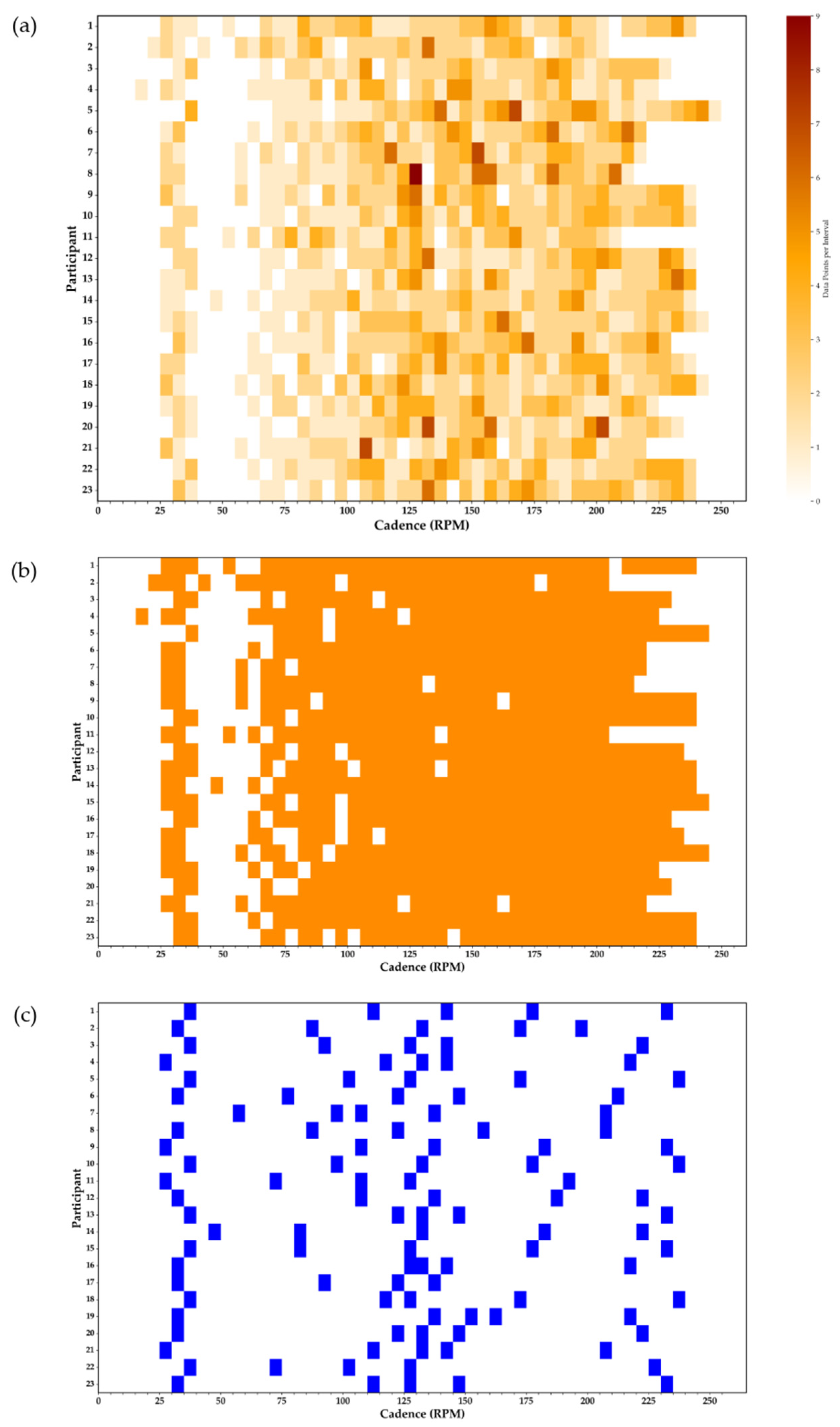
  • Moderate-Number (MN) model: Included only the point with the highest positive residual (i.e., furthest above the fitted curve) in each 5-RPM cadence interval. This method, previously described [5], is intended to eliminate submaximal points and retain the most likely maximal point per interval (Figure 1b and Figure 2c, Table 1). On average, MN models included 34 ± 2 data points per participant (about 40% of the HN dataset).
  • Low-Number (LN) model: Included only five data points selected from strategic portions of the power–cadence relationship to ensure proper representation of three critical regions: (i) low cadences to inform the linear coefficient (ax), (ii) near the apex to capture peak curvature (bx2), and (iii) high cadences to define the descending portion of the curve (cx3). These data points were selected as (i) the point with the highest residual in the low-cadence range (0–60 rpm), (ii) the point of peak power output (Ppeak), the point with the highest residual 5–50 rpm below Ppeak cadence (left side of the apex), and the point with the highest residual 5–50 rpm above Ppeak cadence (right side of the apex), and (iii) the point with the highest residual within 10 rpm of the maximal cadence recorded during the flywheel-only sprint. This method was designed to capture strategically located maximal values for optimal estimation of Equation (1) coefficients (Figure 1c and Figure 2d, Table 1).
In total, 69 third-order polynomial models were generated (23 participants × 3 datasets). For each model, curve goodness of fit was evaluated using the coefficient of determination (R2) and the standard error of the estimate (SEE). From each fitted equation, the x- and y-coordinates of the apex were extracted, corresponding to optimal cadence (Copt) and maximal power (Pmax), respectively. To further assess model accuracy, we calculated additional error metrics, including the mean absolute error (MAE), the mean absolute percentage error (MAPE), and the standard deviation (SD) of the prediction error. We also generated a Bland–Altman plot to visualize the agreement between modeled and experimentally measured peak power (Ppeak), reporting bias, and 95% limits of agreement.
We also assessed the robustness of the LN model to data point selection by conducting a leave-one-out (LOO) sensitivity analysis. Specifically, we generated three additional LN models using only four of the five selected data points by systematically omitting: (i) the low-cadence point (0–60 rpm), (ii) one of the medium-cadence points (Ppeak, or the points 5–50 rpm below or above Ppeak cadence), or (iii) the high-cadence point (within 10 rpm of maximal cadence). For each model, Ppeak was estimated using the known cadence at Ppeak (Cppeak), and both absolute and relative prediction errors were calculated to evaluate model stability.
The statistical analysis focused on comparing (1) curve fit (R2 and SEE), (2) the estimated values of Pmax and Copt, and (3) the ability of each model to accurately reproduce the experimentally observed cadence and power at Ppeak. The Shapiro–Wilk test was used to assess the normality of residuals. If parametric assumptions were met, repeated measures ANOVA was used; otherwise, Friedman’s test was applied. Pairwise comparisons were performed using paired t-tests or Wilcoxon signed-rank tests with Bonferroni correction. Effect sizes were reported using generalized eta squared (η2) for ANOVA and Kendall’s W for Friedman’s test. All analyses were conducted in R (version 4.4.2) using the rstatix and tidyverse packages, with statistical significance set at p < 0.05.

3. Results

3.1. Goodness of Fit of the Models

Model type had a significant and large effect on R2 values (F1.36, 29.92 = 85.63; p < 0.001; η2 = 0.63). The LN model yielded the highest R2 values (0.995 ± 0.008), followed by the MN and HN models. Similarly, a significant and large effect was observed for SEE values (F1.42, 31.29 = 59.39; p < 0.001; η2 = 0.57), with the LN model producing the lowest SEE (29 ± 15 W). Post-hoc comparisons confirmed that the LN model significantly outperformed both the MN and HN models on both metrics (p < 0.001, Bonferroni-adjusted). These results indicate that the LN model provided the best overall goodness of fit, as reflected by both the highest R2 and lowest SEE values. As illustrated in Figure 1c and Figure 2d, this model was based on a minimal number of strategically selected data points representing each participant’s maximal effort across distinct regions of the power–cadence curve. This approach appears particularly well-suited for researchers and practitioners seeking to model maximal performance across the full cadence spectrum. The LN modeling approach provided a better fit and improved estimation of truly maximal power levels across five key cadence regions in young, recreationally active male participants.
The MN model produced intermediate R2 values consistent with prior studies using a similar modeling approach [5], though with slightly higher SEE (53 ± 14 W), likely due to the inclusion of submaximal data points. In many cases, selecting the highest point within a 5-RPM bin captured only a single available value, which may not have reflected a true maximal effort (Figure 2c).
Interestingly, the SEE observed in the LN model here (~30 W) is comparable to SEE values reported previously for MN models in similar populations [5]. This suggests that in populations where consistent maximal effort is difficult to achieve across all cadences, a reduced but strategically filtered dataset may offer a more accurate and efficient alternative.

3.2. Optimal Cadence (Copt): X-Coordinate of the Curve Apex

A significant but small effect of model type was found for Copt values (F1.29, 28.27 = 5.54; p < 0.001; η2 = 0.01). Post-hoc comparisons revealed a significant difference between the LN and MN models (p < 0.01), while the HN model did not differ significantly from either. As shown in Figure 3b, Copt values consistently differed from the cadence at which Ppeak was experimentally measured, with participant-level differences ranging from −21 to +26 RPM. These results support prior findings and reinforce the distinction between cadence at Ppeak and Copt [5], confirming that Copt cannot be directly inferred from the cadence at which peak power was observed experimentally.

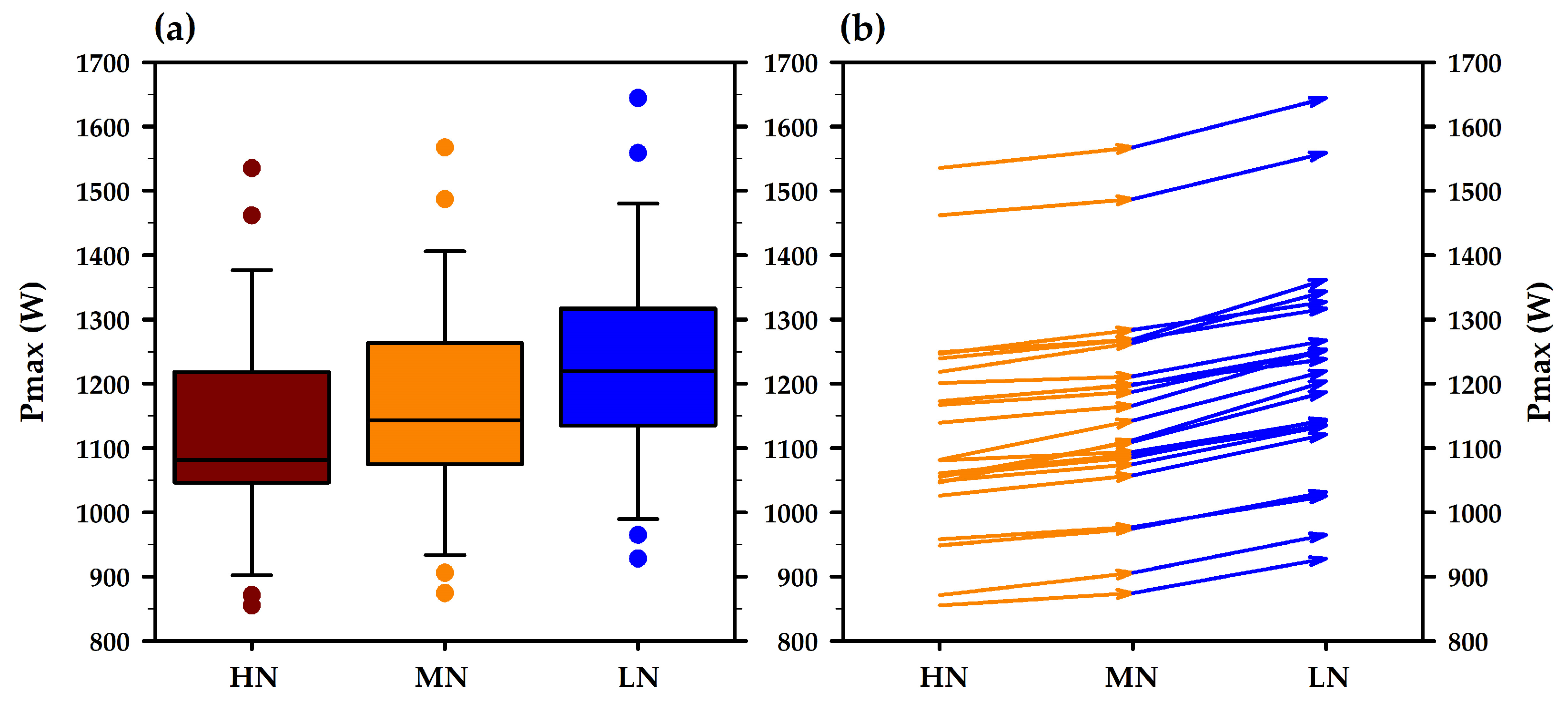
3.3. Modeled Maximal Power Output (Pmax): Y-Coordinate of the Curve Apex

Because residuals for Pmax violated normality, a nonparametric Friedman test was used to assess the effect of model type. A significant difference was found (χ2(2) = 46.00; p < 0.001; Kendall’s W = 1), and post-hoc comparisons indicated that Pmax values differed significantly between all model pairs.
The LN model produced the highest Pmax values (Figure 4), followed by the MN and HN models. Notably, Pmax values increased systematically as the number of modeling points decreased. Compared to the HN model, LN-derived Pmax was 8.5 ± 2.5% higher on average. This difference is similar in magnitude to short-term gains attributed to familiarization effects in prior work: ~11% [23], ~7% [24], and ~4% [21]. Our findings suggest that such gains may partially reflect improved consistency in maximal effort production across pedal cycles.

3.4. Accuracy of the Models for Predicting Ppeak

Given the consistent mismatch between Copt and the cadence at which Ppeak was observed, we assessed model accuracy by comparing the modeled power output at the cadence corresponding to Ppeak (Figure 5).
The LN model demonstrated superior performance, yielding the lowest measurement errors (MAE = 17.8 W; MAPE = 1.45%; SD = 19.2 W), compared to the MN (MAE = 59.3 W; MAPE = 5.12%; SD = 25.1 W) and HN models (MAE = 88.1 W; MAPE = 7.33%; SD = 29.6 W). These findings were further supported by a Bland–Altman analysis (Figure 5), which compared the modeled power to experimentally measured Ppeak. The LN model exhibited the smallest bias (−8 W) and the narrowest limits of agreement (−45 to +29 W), indicating strong agreement and minimal systematic error. In contrast, the MN and HN models showed larger biases and broader limits of agreement, reflecting greater inaccuracies and inconsistencies in predicting Ppeak.

3.5. Sensitivity Analysis of the LN Model

Friedman tests were used to compare prediction errors across removal conditions. No significant differences were found in either absolute prediction error (χ2 = 0.609, df = 2, p = 0.738) or relative prediction error (χ2 = 0.609, df = 2, p = 0.738), indicating that the performance of the LN model was stable regardless of which data point was omitted. Removal of the high-cadence point produced slightly larger mean errors. However, all conditions yielded prediction errors below 11 W on average, with relative errors generally under 2% (Figure 6).

4. Discussion

The main finding of this study is that a better fit of the meaningful data points collected during the Force–Velocity test and a more accurate estimate of Pmax can be obtained using models built on five data points selected to reflect participants’ maximal power-producing capacity, drawn from strategic regions of the power–cadence relationship known to influence the coefficients of third-order polynomial regressions. The Low-Number of data points (LN) model introduced here was specifically designed to help researchers and practitioners model power–cadence relationships after excluding non-maximal data points that are frequently recorded during force–velocity testing (Figure 2). By relying on only five carefully selected points, the LN model captured participants’ maximal power-producing capacity across a wide range of cadences more effectively than a model that included all data points and the model we previously proposed [5].
Our results highlight the need for both the research and applied communities; including strength and conditioning professionals, athletic trainers, and clinicians; to re-evaluate the procedures used to process the data collected from Force–Velocity testing on a stationary cycle ergometer. We argue that future modeling procedures should prioritize distinguishing genuine cadence-specific maximal power levels from the biological noise that often contaminates raw data [5]. The LN modeling method was built around this principle and appears to provide a more valid means of quantifying Pmax in young and physically active male adults [4,20,22,25,26,34,39].
Our results show that the quality of the model fit improved as the number of data points used to characterize the power–cadence curve decreased and the likelihood that those points were truly maximal increased. This was demonstrated by significant and large effects of model type on both R2 and SEE values (Figure 2, Table 2), with the LN model yielding the highest R2 (0.995 ± 0.008) and lowest SEE (29 ± 15 W). These findings build upon our previous methodological recommendations [5], which emphasized the need to capture the complexity of the power–cadence relationship using third-order polynomial models while avoiding the inclusion of submaximal data points that are inevitably recorded during force–velocity tests.
It is also important to consider how testing protocol design and participant characteristics influence the quality and usefulness of the data collected. As illustrated in Figure 1, our protocol yielded relatively few data points at low cadences, while considerable variation in power values across similar cadences suggested that participants were unable to produce cadence-specific maximal power consistently during each pedal cycle (see Figure 2). These limitations are consistent with previous observations [5,6,7,21,22,28,34,38,39], though they have not been systematically analyzed. Our findings reinforce earlier recommendations [5] that researchers and practitioners focus on the collection of truly maximal data points, with special attention to ensuring that such data points are recorded at strategically important cadences to optimize model fit.
Our results support the use of the LN model for a more valid and reliable estimation of Pmax; a variable of critical relevance when assessing neuromuscular function in both performance [6,7,8,9,10,11,12,13,14,15], or clinical settings [20,21]. The LN model yielded the closest estimates to experimentally observed peak power output (MAE = 17.8 W; MAPE = 1.45%; SD = 19.2 W), significantly outperforming both the HN and MN models and showing a strong agreement and no systematic bias for the population tested in this study (Figure 5). To assess model validity, we recommend that researchers and practitioners conduct a simple visual inspection of the data points and the fitted curve. Since Pmax represents the theoretical maximum power an individual can produce, and is only achievable at a single cadence, models that yield Pmax values substantially lower than Ppeak should be interpreted with caution. We also encourage practitioners to use the LN model when familiarization sessions cannot be implemented [21,23,24].
The LN model not only outperformed the widely used HN model, which includes all available data points regardless of quality, but also provided better estimates than the MN model we previously developed [5]. It is worth noting that we observed similar goodness-of-fit for the LN models used in this study and the MN models in our previous work. We posit that LN models may yield superior results, particularly when analyzing data from individuals who demonstrate greater variability in motor command during Force–Velocity testing. Furthermore, our sensitivity analysis demonstrated that even when reduced to four strategically selected maximal data points, the LN model maintained high accuracy in predicting Ppeak; however, we recommend that researchers and practitioners make every effort to include a maximal effort at high cadence, as the model showed slightly increased sensitivity when that point was omitted.
An important limitation of the present study is the homogeneity of the participant sample, which included only young, recreationally active male individuals. The accuracy and applicability of the five-point data selection strategy may differ across populations with distinct physiological or neuromuscular characteristics. For example, individuals with neuromuscular impairments, older adults, or younger individuals may display greater variability in power output across pedal cycles, making it more challenging to identify five truly maximal data points across the power–cadence relationship. Future research should examine the generalizability and robustness of the proposed modeling approach in more diverse populations. Another limitation is that the test-retest reliability of the modeling approach was not assessed, as data were not collected across multiple sessions. Evaluating the consistency of the model outputs over time is essential to confirm the robustness and practical utility of the five-point selection strategy, and this should also be addressed in future research. Additionally, we acknowledge that our selection strategy may face ambiguity in rare cases where multiple data points within a defined cadence range yield similar residuals. In such instances, we recommend prioritizing points with the highest residuals at lower cadences to optimize the estimation of the a coefficient, and those at higher cadences to refine the estimation of the c coefficient (see Equation (1) of the third order polynomials). On both limbs of the power–cadence curve, selecting the point with the highest residual at the extreme end of the cadence range helps ensure that the selected data point lies further outside the curve and is more likely to reflect a truly maximal effort.

5. Conclusions

Selecting only five, or even four, maximal data points at strategically selected cadences provides a robust approach to modeling power–cadence relationships during cycling, particularly in controlled laboratory settings where conditions are typically more conducive to obtaining high-quality data. This approach, based on both physiological understanding and modeling rationale, can lead to a more accurate assessment of Pmax in such environments. The LN model offers a practical, easy-to-implement solution to minimize the influence of biological noise associated with movement variability on the experimental data used to characterize power-cadence relationships during Force–Velocity testing on a stationary cycle ergometer. From a practical standpoint, the results obtained using the LN modeling approach may help reduce the overall duration of Force–Velocity testing while increasing the likelihood of obtaining high-quality data points. Specifically, we encourage researchers and practitioners to prioritize three maximal efforts: one initiated from a stationary start against heavy resistance (to capture a lot of data points on the left end of the curve and inform the a coefficient), one initiated from a rolling start at approximately 70 rpm against moderate resistance (to capture a lot of data points around the apex of the curve and inform the b coefficient), and one initiated from a rolling start at approximately 140 rpm against low resistance (to capture a lot of data points on the right end of the curve and inform the c coefficient). This targeted approach ensures comprehensive coverage of key cadence ranges required for third-order polynomial modeling while maximizing the likelihood of collecting truly maximal data points.

Author Contributions

Conceptualization, D.M.R.; methodology, D.M.R., B.L.R. and C.A.H.; formal analysis, D.M.R. and M.W.D.; investigation, D.M.R. and C.A.H.; data curation, T.A.; writing—original draft preparation, D.M.R.; writing—review and editing, D.M.R., B.L.R., M.W.D. and T.A.; visualization, D.M.R.; supervision, D.M.R. All authors have read and agreed to the published version of the manuscript.

Funding

This research received no external funding.

Institutional Review Board Statement

Ethical review and approval were waived for this study, as it was classified as non-interventional research involving no additional or unusual procedures for diagnosis, treatment, or monitoring. All procedures were standard, consistent with established practices in exercise testing, and conducted in accordance with the principles of the Declaration of Helsinki.

Informed Consent Statement

Informed consent for participation was obtained from all subjects involved in the study.

Data Availability Statement

The original contributions presented in this study are included in the article. Further inquiries can be directed to the corresponding author.

Acknowledgments

The authors would like to acknowledge Sylvain Dorel for his assistance during data collection, Muriel Bourdin for access to the ergometer used for the experiments. The corresponding author would also like to acknowledge the in-kind support provided by Ayrton and Naomi, whose patience helped bring balance to the writing process. During the preparation of this manuscript/study, the author(s) used ChatGPT o4-mini-high for the purposes of developing scripts for the analysis of the data using Python (version 3.12). The authors have reviewed and edited the output and take full responsibility for the content of this publication.

Conflicts of Interest

The authors declare no conflicts of interest.

Abbreviations

The following abbreviations are used in this manuscript:
CppeakCadence at the highest level of power measured experimentally
Coptx-coordinate of the apex of the modeled power vs. cadence relationship
HNHigh-number of data points model
LNLow-number of data points model
LLOLeave-One-Out sensitivity analysis
MAEMean Absolute Error
MAPEMean Absolute Percentage Error
MNModerate-number of data points model
Pmaxy-coordinate of the apex of the modeled power vs. cadence relationship
PpeakHighest level of power measured experimentally
RPMRotation per minute
SEEStandard Error of the Estimate
WWatt

References

  1. Dotan, R.; Bar-Or, O. Load optimization for the Wingate Anaerobic Test. Eur. J. Appl. Physiol. Occup. Physiol. 1983, 51, 409–417. [Google Scholar] [CrossRef] [PubMed]
  2. Driss, T.; Vandewalle, H. The measurement of maximal (anaerobic) power output on a cycle ergometer: A critical review. Biomed. Res. Int. 2013, 2013, 589361. [Google Scholar] [CrossRef]
  3. Sargeant, A.J.; Dolan, P.; Young, A. Optimal Velocity for Maximal Short-term (Anaerobic) Power Output in Cycling. Int. J. Sports Med. 1984, 5, 124–125. [Google Scholar] [CrossRef]
  4. Vandewalle, H.; Peres, G.; Heller, J.; Monod, H. All out anaerobic capacity tests on cycle ergometers. A comparative study on men and women. Eur. J. Appl. Physiol. Occup. Physiol. 1985, 54, 222–229. [Google Scholar] [CrossRef]
  5. Rudsits, B.L.; Hopkins, W.G.; Hautier, C.A.; Rouffet, D.M. Force-velocity test on a stationary cycle ergometer: Methodological recommendations. J. Appl. Physiol. 2018, 124, 831–839. [Google Scholar] [CrossRef]
  6. Bertucci, W.; Taiar, R.; Grappe, F. Differences between sprint tests under laboratory and actual cycling conditions. J. Sports Med. Phys. Fit. 2005, 45, 277–283. [Google Scholar]
  7. Dorel, S.; Hautier, C.A.; Rambaud, O.; Rouffet, D.; Van Praagh, E.; Lacour, J.R.; Bourdin, M. Torque and power-velocity relationships in cycling: Relevance to track sprint performance in world-class cyclists. Int. J. Sports Med. 2005, 26, 739–746. [Google Scholar] [CrossRef]
  8. Gardner, A.S.; Martin, J.C.; Martin, D.T.; Barras, M.; Jenkins, D.G. Maximal torque- and power-pedaling rate relationships for elite sprint cyclists in laboratory and field tests. Eur. J. Appl. Physiol. 2007, 101, 287–292. [Google Scholar] [CrossRef]
  9. Vandewalle, H.; Peres, G.; Heller, J.; Panel, J.; Monod, H. Force-velocity relationship and maximal power on a cycle ergometer. Correlation with the height of a vertical jump. Eur. J. Appl. Physiol. Occup. Physiol. 1987, 56, 650–656. [Google Scholar] [CrossRef]
  10. Wackwitz, T.A.; Minahan, C.L.; King, T.; Du Plessis, C.; Andrews, M.H.; Bellinger, P.M. Quantification of maximal power output in well-trained cyclists. J. Sports Sci. 2021, 39, 84–90. [Google Scholar] [CrossRef]
  11. Yeo, B.K.; Rouffet, D.M.; Bonanno, D.R. Foot orthoses do not affect crank power output during maximal exercise on a cycle-ergometer. J. Sci. Med. Sport. 2016, 19, 368–372. [Google Scholar] [CrossRef] [PubMed]
  12. Dwyer, D.B.; Molaro, C.; Rouffet, D.M. Force-velocity profiles of track cyclists differ between seated and non-seated positions. Sports Biomech. 2023, 22, 621–632. [Google Scholar] [CrossRef]
  13. Taylor, K.B.; Deckert, S.; Sanders, D. Field-testing to determine power—and torque—cadence profiles in professional road cyclists. Eur. J. Sport. Sci. 2023, 23, 1085–1093. [Google Scholar] [CrossRef] [PubMed]
  14. Crielaard, J.M.; Pirnay, F. Anaerobic and aerobic power of top athletes. Eur. J. Appl. Physiol. Occup. Physiol. 1981, 47, 295–300. [Google Scholar] [CrossRef]
  15. Kordi, M.; Folland, J.; Goodall, S.; Barratt, P.; Howatson, G. Isovelocity vs. Isoinertial Sprint Cycling Tests for Power- and Torque-cadence Relationships. Int. J. Sports Med. 2019, 40, 897–902. [Google Scholar] [CrossRef]
  16. Buttelli, O.; Seck, D.; Vandewalle, H.; Jouanin, J.C.; Monod, H. Effect of fatigue on maximal velocity and maximal torque during short exhausting cycling. Eur. J. Appl. Physiol. Occup. Physiol. 1996, 73, 175–179. [Google Scholar] [CrossRef]
  17. Gardner, A.S.; Martin, D.T.; Jenkins, D.G.; Dyer, I.; Van Eiden, J.; Barras, M.; Martin, J.C. Velocity-specific fatigue: Quantifying fatigue during variable velocity cycling. Med. Sci. Sports Exerc. 2009, 41, 904–911. [Google Scholar] [CrossRef]
  18. McCartney, N.; Heigenhauser, G.J.; Jones, N.L. Power output and fatigue of human muscle in maximal cycling exercise. J. Appl. Physiol. Respir. Environ. Exerc. Physiol. 1983, 55, 218–224. [Google Scholar] [CrossRef]
  19. O’Bryan, S.J.; Taylor, J.L.; D’Amico, J.M.; Rouffet, D.M. Quadriceps Muscle Fatigue Reduces Extension and Flexion Power During Maximal Cycling. Front. Sports Act. Living 2021, 3, 797288. [Google Scholar] [CrossRef]
  20. Davies, C.T.; Young, K. Effects of external loading on short term power output in children and young male adults. Eur. J. Appl. Physiol. Occup. Physiol. 1984, 52, 351–354. [Google Scholar] [CrossRef]
  21. Doré, E.; Duché, P.; Rouffet, D.; Ratel, S.; Bedu, M.; Van Praagh, E. Measurement error in short-term power testing in young people. J. Sports Sci. 2003, 21, 135–142. [Google Scholar] [CrossRef]
  22. Arsac, L.M.; Belli, A.; Lacour, J.R. Muscle function during brief maximal exercise: Accurate measurements on a friction-loaded cycle ergometer. Eur. J. Appl. Physiol. Occup. Physiol. 1996, 74, 100–106. [Google Scholar] [CrossRef] [PubMed]
  23. Capriotti, P.V.; Sherman, W.M.; Lamb, D.R. Reliability of power output during intermittent high-intensity cycling. Med. Sci. Sports Exerc. 1999, 31, 913–915. [Google Scholar] [CrossRef]
  24. Martin, J.C.; Diedrich, D.; Coyle, E.F. Time course of learning to produce maximum cycling power. Int. J. Sports Med. 2000, 21, 485–487. [Google Scholar] [CrossRef]
  25. Davies, C.T.; Sandstrom, E.R. Maximal mechanical power output and capacity of cyclists and young adults. Eur. J. Appl. Physiol. Occup. Physiol. 1989, 58, 838–844. [Google Scholar] [CrossRef]
  26. Driss, T.; Vandewalle, H.; Chevalier, J.M.L.; Monod, H. Force-velocity relationship on a cycle ergometer and knee-extensor strength indices. Can. J. Appl. Physiol. 2002, 27, 250–262. [Google Scholar] [CrossRef]
  27. Driss, T.; Vandewalle, H.; Monod, H. Maximal power and force-velocity relationships during cycling and cranking exercises in volleyball players. Correlation with the vertical jump test. J. Sports Med. Phys. Fit. 1998, 38, 286–293. [Google Scholar]
  28. Seck, D.; Vandewalle, H.; Decrops, N.; Monod, H. Maximal power and torque-velocity relationship on a cycle ergometer during the acceleration phase of a single all-out exercise. Eur. J. Appl. Physiol. Occup. Physiol. 1995, 70, 161–168. [Google Scholar] [CrossRef]
  29. Dorel, S.; Couturier, A.; Lacour, J.R.; Vandewalle, H.; Hautier, C.; Hug, F. Force-velocity relationship in cycling revisited: Benefit of two-dimensional pedal forces analysis. Med. Sci. Sports Exerc. 2010, 42, 1174–1183. [Google Scholar] [CrossRef]
  30. Kruger, R.L.; Peyrard, A.; di Domenico, H.; Rupp, T.; Millet, G.Y.; Samozino, P. Optimal load for a torque-velocity relationship test during cycling. Eur. J. Appl. Physiol. 2020, 120, 2455–2466. [Google Scholar] [CrossRef]
  31. Nadeau, M.; Brassard, A.; Cuerrier, J.P. The bicycle ergometer for muscle power testing. Can. J. Appl. Sport. Sci. 1983, 8, 41–46. [Google Scholar]
  32. Leo, P.; Martinez-Gonzalez, B.; Mujika, I.; Giorgi, A. Mechanistic influence of the torque cadence relationship on power output during exhaustive all-out field tests in professional cyclists. J. Sports Sci. 2025, 43, 887–894. [Google Scholar] [CrossRef] [PubMed]
  33. Bogdanis, G.C.; Papaspyrou, A.; Theos, A.; Maridaki, M. Influence of resistive load on power output and fatigue during intermittent sprint cycling exercise in children. Eur. J. Appl. Physiol. 2007, 101, 313–320. [Google Scholar] [CrossRef] [PubMed]
  34. Capmal, S.; Vandewalle, H. Torque-velocity relationship during cycle ergometer sprints with and without toe clips. Eur. J. Appl. Physiol. Occup. Physiol. 1997, 76, 375–379. [Google Scholar] [CrossRef]
  35. Linossier, M.T.; Denis, C.; Dormois, D.; Geyssant, A.; Lacour, J.R. Ergometric and metabolic adaptation to a 5-s sprint training programme. Eur. J. Appl. Physiol. Occup. Physiol. 1993, 67, 408–414. [Google Scholar] [CrossRef]
  36. Martin, J.C.; Wagner, B.M.; Coyle, E.F. Inertial-load method determines maximal cycling power in a single exercise bout. Med. Sci. Sports Exerc. 1997, 29, 1505–1512. [Google Scholar] [CrossRef]
  37. McCartney, N.; Obminski, G.; Heigenhauser, G.J. Torque-velocity relationship in isokinetic cycling exercise. J. Appl. Physiol. 1985, 58, 1459–1462. [Google Scholar] [CrossRef]
  38. Sargeant, A.J.; Hoinville, E.; Young, A. Maximum leg force and power output during short-term dynamic exercise. J. Appl. Physiol. Respir. Environ. Exerc. Physiol. 1981, 51, 1175–1182. [Google Scholar] [CrossRef]
  39. Hautier, C.A.; Linossier, M.T.; Belli, A.; Lacour, J.R.; Arsac, L.M. Optimal velocity for maximal power production in non-isokinetic cycling is related to muscle fibre type composition. Eur. J. Appl. Physiol. Occup. Physiol. 1996, 74, 114–118. [Google Scholar] [CrossRef]
  40. Rouffet, D.M. Étude de L’activation Musculaire À L’aide de L’électromyographie de Surface—Aspects Méthodologiques et Apports Dans L’analyse du Mouvement Humain. Ph.D. Thesis, Université Claude Bernard Lyon 1, Villeurbanne, France, 2007. [Google Scholar]
  41. Lakomy, H.K. Measurement of work and power output using friction-loaded cycle ergometers. Ergonomics 1986, 29, 509–517. [Google Scholar] [CrossRef]
  42. Morin, J.B.; Belli, A. A simple method for measurement of maximal downstroke power on friction-loaded cycle ergometer. J. Biomech. 2004, 37, 141–145. [Google Scholar] [CrossRef] [PubMed]
Figure 1. Heatmaps showing the distribution of data points used to build the power–cadence models for each participant across 5-RPM cadence intervals. (a) High-Number (HN) model includes all available data points. (b) Moderate-Number (MN) model includes the maximal power value recorded within each 5-RPM interval. (c) Low-Number (LN) model includes five data points selected using a residual-based filtering method from key regions of the power–cadence curve. Each row represents one participant; colors indicate the presence or frequency of data points within each interval.
Signals 06 00032 g001
Figure 2. Illustration of experimental data points and models for a representative participant. (a) All data points recorded during testing. (b) High-Number (HN) model constructed using all experimental data points. (c) Moderate-Number (MN) model constructed using one point per 5-RPM cadence bin. (d) Low-Number (LN) model constructed using five maximal data points strategically distributed along the power–cadence curve. The experimental data corresponding to Ppeak (peak power), as well as the x- and y-coordinates of the apex of the power vs. cadence relationships are shown for each model.
Signals 06 00032 g002
Figure 3. (a) Boxplot showing the distribution of Copt values estimated from the three modeling approaches. Asterisks (*) indicate a significant difference between Low-Number (LN) and Moderate-Number (MN) models. (b) Bar plot illustrating individual differences between the cadence at which Ppeak (peak power) was measured and the Copt (Optimal cadence) value derived from the Low-Number (LN) model for each participant (n = 23).
Signals 06 00032 g003
Figure 4. (a) Boxplot showing Pmax values derived from each model. Pmax increases with reduced dataset size. (b) Vector plot showing participant-level changes in Pmax when switching from the High-Number (HN) to the Moderate-Number (MN) and the Low-Number (LN) model, highlighting the benefit of selecting five high-quality, strategically placed data points.
Signals 06 00032 g004
Figure 5. Bland–Altman plot assessing agreement between Ppeak (peak power) derived from the High-Number (HN), Moderate-Number (MN) and Low-Number (LN) models and experimentally measured during the Force–Velocity test. The dotted lines represents the mean prediction error (bias), while the dashed lines show the 95% limits of agreement (±1.96 SD). All differences but one fall within these limits, indicating strong agreement between the modeled and measured values obtained from all three models. The HN and MN models exhibit systematic bias across the range of measured values, whereas the LN model shows no such trend, indicating more consistent agreement with the experimental data.
Signals 06 00032 g005
Figure 6. Comparison of LN Model and Leave-One-Out (LOO) Validation Errors in Ppeak Estimation. Bars represent the prediction error (modeled Ppeak—experimental Ppeak) for each participant using: (i) the five-point LN model (blue), which includes the point with the highest residual in the low-cadence range (0–60 rpm), the Ppeak point, the points with the highest residuals 5–50 rpm below and above the Ppeak cadence (left and right of the apex), and the point with the highest residual within 10 rpm of the maximal cadence; (ii) a four-point model with the low-cadence point removed (cyan); (iii) a four-point model with only two of the three medium-cadence points retained (yellow); and (iv) a four-point model with the high-cadence point removed (red).
Signals 06 00032 g006
Table 1. Characteristics of the datasets used to construct the three power–cadence models. Values are expressed as mean ± standard deviation. “Data points (n)” indicates the number of points used in each model. “Min cadence” and “Max cadence” correspond to the lowest and highest cadences (in RPM, rotations per minute) included. HN = High-Number model; MN = Moderate-Number model; LN = Low-Number model.
HNMNLN
Data points (n)81 ± 734 ± 25 ± 0
Min cadence (RPM)31 ± 333 ± 235 ± 6
Max cadence (RPM)229 ± 12229 ± 12216 ± 23
Table 2. Summary of metrics used to assess model fit and performance. Values are presented as mean ± standard deviation. R2 = coefficient of determination; SEE = standard error of the estimate; Pmax = modeled maximal power output; Copt = optimal cadence (x-coordinate of the apex of the curve). “Exp. Data” refers to the experimentally measured power peak (Ppeak) and its associated cadence (Cppeak). HN = High-Number model; MN = Moderate-Number model; LN = Low-Number model.
Exp. DataHNMNLN
R2 0.938 ± 0.0270.962 ± 0.0140.995 ± 0.008
SEE (W) 72 ± 1753 ± 1429 ± 15
Ppeak/Pmax (W)1218 ± 1781126 ± 1631157 ± 1621220 ± 168
Cppeak/Copt (RPM)127 ± 11125 ± 8127 ± 8126 ± 8
Disclaimer/Publisher’s Note: The statements, opinions and data contained in all publications are solely those of the individual author(s) and contributor(s) and not of MDPI and/or the editor(s). MDPI and/or the editor(s) disclaim responsibility for any injury to people or property resulting from any ideas, methods, instructions or products referred to in the content.

