
Comparative Analysis of Attention Mechanisms in Densely Connected Network for Network Traffic Prediction

 , , ,
, , ,
Abstract
1. Introduction
- We propose ADNet, based on STDenseNet, which is designed through searches for optimal types and positions of attention modules.
- We conduct comprehensive experiments and several ablation experiments to validate effectiveness. By applying our method, we can achieve remarkable prediction performance compared with existing methods.
2. Related Works
2.1. Convolutional Network for Network Traffic Prediction
2.2. Attention Mechanism
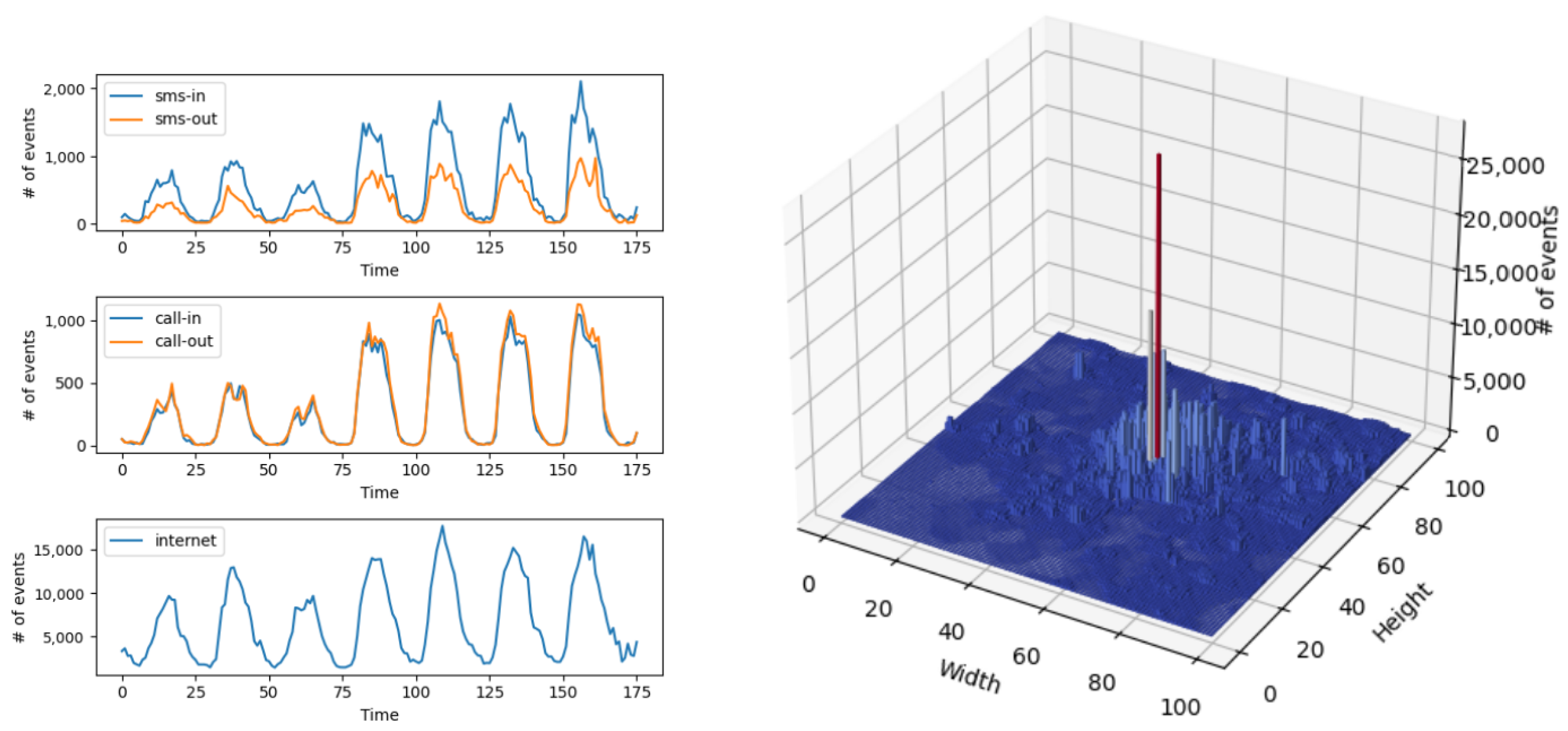
3. Data Analysis
4. Method
4.1. Overview
4.2. Feature Extraction in Closeness and Period
4.3. Attention Module
4.4. Parametric Matrix Based Fusion
5. Experiment
5.1. Experiment Setting
5.1.1. Dataset Preprocessing
5.1.2. Experimental Environment
5.2. Result
5.3. Efficiency of Attention Module
5.4. Position of Attention Module
6. Conclusions
Supplementary Materials
Author Contributions
Funding
Data Availability Statement
Conflicts of Interest
References
- Park, Y.; Park, A.; Kang, S.; Kim, Y.; Ryu, S. Trends on Development of Network Capacity in LTE-Advanced to Support Increasing Mobile Data Traffic. Electron. Telecommun. Trends 2012, 27, 122–135. [Google Scholar]
- Le, D.H.; Tran, H.A.; Souihi, S.; Mellouk, A. An AI-based traffic matrix prediction solution for software-defined network. In Proceedings of the ICC 2021—IEEE International Conference on Communications, Montreal, QC, Canada, 14–23 June 2021; pp. 1–6. [Google Scholar]
- Zhu, Y.; Wang, S. Joint traffic prediction and base station sleeping for energy saving in cellular networks. In Proceedings of the ICC 2021—IEEE International Conference on Communications, Montreal, QC, Canada, 14–23 June 2021; pp. 1–6. [Google Scholar]
- Wu, Q.; Chen, X.; Zhou, Z.; Chen, L.; Zhang, J. Deep reinforcement learning with spatio-temporal traffic forecasting for data-driven base station sleep control. IEEE/ACM Trans. Netw. 2021, 29, 935–948. [Google Scholar] [CrossRef]
- Lin, J.; Chen, Y.; Zheng, H.; Ding, M.; Cheng, P.; Hanzo, L. A data-driven base station sleeping strategy based on traffic prediction. IEEE Trans. Netw. Sci. Eng. 2021, 11, 5627–5643. [Google Scholar] [CrossRef]
- Saxena, N.; Sahu, B.J.; Han, Y.S. Traffic-aware energy optimization in green LTE cellular systems. IEEE Commun. Lett. 2013, 18, 38–41. [Google Scholar] [CrossRef]
- Liu, B.; Meng, F.; Zhao, Y.; Qi, X.; Lu, B.; Yang, K.; Yan, X. A linear regression-based prediction method to traffic flow for low-power WAN with smart electric power allocations. In Simulation Tools and Techniques, Proceedings of the 11th International Conference, SIMUtools 2019, Chengdu, China, 8–10 July 2019; Song, H., Jiang, D., Eds.; Proceedings 11; Springer International Publishing: Cham, Switzerland, 2019; pp. 125–134. [Google Scholar] [CrossRef]
- Sun, H.; Liu, H.X.; Xiao, H.; He, R.R.; Ran, B. Use of local linear regression model for short-term traffic forecasting. Transp. Res. Rec. 2003, 1836, 143–150. [Google Scholar] [CrossRef]
- Rizwan, A.; Arshad, K.; Fioranelli, F.; Imran, A.; Imran, M.A. Mobile internet activity estimation and analysis at high granularity: SVR model approach. In Proceedings of the 2018 IEEE 29th Annual International Symposium on Personal, Indoor and Mobile Radio Communications (PIMRC), Bologna, Italy, 9–12 September 2018; pp. 1–7. [Google Scholar]
- Cong, Y.; Wang, J.; Li, X. Traffic flow forecasting by a least squares support vector machine with a fruit fly optimization algorithm. Procedia Eng. 2016, 137, 59–68. [Google Scholar] [CrossRef]
- Sapankevych, N.I.; Sankar, R. Time series prediction using support vector machines: A survey. IEEE Comput. Intell. Mag. 2009, 4, 24–38. [Google Scholar] [CrossRef]
- Tian, Y.; Wei, C.; Xu, D. Traffic flow prediction based on stack autoencoder and long short-term memory network. In Proceedings of the 2020 IEEE 3rd International Conference on Automation, Electronics and Electrical Engineering (AUTEEE), Shenyang, China, 20–22 November 2020; pp. 385–388. [Google Scholar] [CrossRef]
- Wang, J.; Tang, J.; Xu, Z.; Wang, Y.; Xue, G.; Zhang, X.; Yang, D. Spatiotemporal modeling and prediction in cellular networks: A big data enabled deep learning approach. In Proceedings of the IEEE INFOCOM 2017—IEEE Conference on Computer Communications, Atlanta, GA, USA, 1–4 May 2017; pp. 1–9. [Google Scholar] [CrossRef]
- Zhang, C.; Zhang, H.; Yuan, D.; Zhang, M. Citywide cellular traffic prediction based on densely connected convolutional neural networks. IEEE Commun. Lett. 2018, 22, 1656–1659. [Google Scholar] [CrossRef]
- Zhang, D.; Liu, L.; Xie, C.; Yang, B.; Liu, Q. Citywide cellular traffic prediction based on a hybrid spatiotemporal network. Algorithms 2020, 13, 20. [Google Scholar] [CrossRef]
- Zhang, J.; Zheng, Y.; Qi, D. Deep spatio-temporal residual networks for citywide crowd flows prediction. Proc. AAAI Conf. Artif. Intell. 2017, 31. [Google Scholar] [CrossRef]
- Chen, C.; Li, K.; Teo, S.G.; Zou, X.; Li, K.; Zeng, Z. Citywide traffic flow prediction based on multiple gated spatio-temporal convolutional neural networks. ACM Trans. Knowl. Discov. Data TKDD 2020, 14, 1–23. [Google Scholar] [CrossRef]
- Sun, S.; Wu, H.; Xiang, L. City-wide traffic flow forecasting using a deep convolutional neural network. Sensors 2020, 20, 421. [Google Scholar] [CrossRef] [PubMed]
- Yang, D.; Li, S.; Peng, Z.; Wang, P.; Wang, J.; Yang, H. MF-CNN: Traffic flow prediction using convolutional neural network and multi-features fusion. IEICE Trans. Inf. Syst. 2019, 102, 1526–1536. [Google Scholar] [CrossRef]
- Zheng, C.; Fan, X.; Wen, C.; Chen, L.; Wang, C.; Li, J. DeepSTD: Mining spatio-temporal disturbances of multiple context factors for citywide traffic flow prediction. IEEE Trans. Intell. Transp. Syst. 2019, 21, 3744–3755. [Google Scholar] [CrossRef]
- Wang, Z.; Wong, V.W. Cellular traffic prediction using deep convolutional neural network with attention mechanism. In Proceedings of the ICC 2022—IEEE International Conference on Communications, Seoul, Republic of Korea, 16–20 May 2022; pp. 2339–2344. [Google Scholar] [CrossRef]
- Huang, G.; Liu, Z.; Van Der Maaten, L.; Weinberger, K.Q. Densely connected convolutional networks. In Proceedings of the IEEE Conference on Computer Vision and Pattern Recognition, Honolulu, HI, USA, 21–26 July 2017; pp. 4700–4708. [Google Scholar]
- Dai, J.; Qi, H.; Xiong, Y.; Li, Y.; Zhang, G.; Hu, H.; Wei, Y. Deformable convolutional networks. In Proceedings of the IEEE International Conference on Computer Vision, Venice, Italy, 22–29 October 2017; pp. 764–773. [Google Scholar]
- Shen, W.; Zhang, H.; Guo, S.; Zhang, C. Time-wise attention aided convolutional neural network for data-driven cellular traffic prediction. IEEE Wirel. Commun. Lett. 2021, 10, 1747–1751. [Google Scholar] [CrossRef]
- Bahdanau, D.; Cho, K.; Bengio, Y. Neural machine translation by jointly learning to align and translate. arXiv 2014, arXiv:1409.0473. [Google Scholar]
- Vaswani, A.; Shazeer, N.; Parmar, N.; Uszkoreit, J.; Jones, L.; Gomez, A.N.; Kaiser, Ł.; Polosukhin, I. Attention is all you need. Adv. Neural Inf. Process. Syst. 2017, 30, 6000–6010. [Google Scholar]
- Wang, X.; Girshick, R.; Gupta, A.; He, K. Non-local neural networks. In Proceedings of the IEEE Conference on Computer Vision and Pattern Recognition, Salt Lake City, UT, USA, 18–23 June 2018; pp. 7794–7803. [Google Scholar]
- Hu, J.; Shen, L.; Sun, G. Squeeze-and-excitation networks. In Proceedings of the IEEE Conference on Computer Vision and Pattern Recognition, Salt Lake City, UT, USA, 18–23 June 2018; pp. 7132–7141. [Google Scholar]
- Mnih, V.; Heess, N.; Graves, A.; Kavukcuoglu, K. Recurrent models of visual attention. Adv. Neural Inf. Process. Syst. 2014, 27, 2204–2212. [Google Scholar]
- Wang, F.; Jiang, M.; Qian, C.; Yang, S.; Li, C.; Zhang, H.; Wang, X.; Tang, X. Residual attention network for image classification. In Proceedings of the IEEE Conference on Computer Vision and Pattern Recognition, Honolulu, HI, USA, 21–26 July 2017; pp. 3156–3164. [Google Scholar]
- Itti, L.; Koch, C.; Niebur, E. A model of saliency-based visual attention for rapid scene analysis. IEEE Trans. Pattern Anal. Mach. Intell. 2002, 20, 1254–1259. [Google Scholar] [CrossRef]
- Woo, S.; Park, J.; Lee, J.Y.; Kweon, I.S. Cbam: Convolutional block attention module. In Proceedings of the European Conference on Computer Vision (ECCV), Munich, Germany, 8–14 September 2018; pp. 3–19. [Google Scholar]
- Misra, D.; Nalamada, T.; Arasanipalai, A.U.; Hou, Q. Rotate to attend: Convolutional triplet attention module. In Proceedings of the IEEE/CVF Winter Conference on Applications of Computer Vision, Virtual Conference, 5–9 January 2021; pp. 3139–3148. [Google Scholar]
- Yao, Y.; Gu, B.; Su, Z.; Guizani, M. MVSTGN: A multi-view spatial-temporal graph network for cellular traffic prediction. IEEE Trans. Mob. Comput. 2021, 22, 2837–2849. [Google Scholar] [CrossRef]
- Xiao, J.; Cong, Y.; Zhang, W.; Weng, W. A cellular traffic prediction method based on diffusion convolutional GRU and multi-head attention mechanism. Clust. Comput. 2025, 28, 125. [Google Scholar] [CrossRef]
- Rao, Z.; Xu, Y.; Pan, S.; Guo, J.; Yan, Y.; Wang, Z. Cellular traffic prediction: A deep learning method considering dynamic nonlocal spatial correlation, self-attention, and correlation of spatiotemporal feature fusion. IEEE Trans. Netw. Serv. Manag. 2022, 20, 426–440. [Google Scholar] [CrossRef]
- Ma, X.; Zheng, B.; Jiang, G.; Liu, L. Cellular network traffic prediction based on correlation ConvLSTM and self-attention network. IEEE Commun. Lett. 2023, 27, 1909–1912. [Google Scholar] [CrossRef]
- Su, J.; Cai, H.; Sheng, Z.; Liu, A.; Baz, A. Traffic prediction for 5G: A deep learning approach based on lightweight hybrid attention networks. Digit. Signal Process. 2024, 146, 104359. [Google Scholar] [CrossRef]
- Yang, H.; Jiang, J.; Zhao, Z.; Pan, R.; Tao, S. STVANet: A spatio-temporal visual attention framework with large kernel attention mechanism for citywide traffic dynamics prediction. Expert Syst. Appl. 2024, 254, 124466. [Google Scholar] [CrossRef]
- Chu, L.; Hou, Z.; Jiang, J.; Yang, J.; Zhang, Y. Spatial-temporal feature extraction and evaluation network for citywide traffic condition prediction. IEEE Trans. Intell. Veh. 2023. [Google Scholar] [CrossRef]
- Barlacchi, G.; De Nadai, M.; Larcher, R.; Casella, A.; Chitic, C.; Torrisi, G.; Antonelli, F.; Vespignani, A.; Pentland, A.; Lepri, B. A multi-source dataset of urban life in the city of Milan and the Province of Trentino. Sci. Data 2015, 2, 150055. [Google Scholar] [CrossRef]
- Telecom Italia. Telecommunications-SMS, Call, Internet-MI. Harvard Dataverse, 2015. V1. Available online: https://dataverse.harvard.edu/dataset.xhtml?persistentId=doi:10.7910/DVN/EGZHFV (accessed on 6 February 2025).
- Wang, X.; Yang, K.; Wang, Z.; Feng, J.; Zhu, L.; Zhao, J.; Deng, C. Adaptive hybrid spatial-temporal graph neural network for cellular traffic prediction. In Proceedings of the ICC 2023-IEEE International Conference on Communications, Rome, Italy, 28 May–1 June 2023; pp. 4026–4032. [Google Scholar] [CrossRef]
- Zhao, N.; Ye, Z.; Pei, Y.; Liang, Y.C.; Niyato, D. Spatial-temporal attention-convolution network for citywide cellular traffic prediction. IEEE Commun. Lett. 2020, 24, 2532–2536. [Google Scholar] [CrossRef]
- Hu, Y.; Zhou, Y.; Song, J.; Xu, L.; Zhou, X. Citywide mobile traffic forecasting using spatial-temporal downsampling transformer neural networks. IEEE Trans. Netw. Serv. Manag. 2022, 20, 152–165. [Google Scholar] [CrossRef]
- Song, B.; Han, B.; Zhang, S.; Ding, J.; Hong, M. Unraveling the gradient descent dynamics of transformers. Adv. Neural Inf. Process. Syst. 2024, 37, 92317–92351. [Google Scholar]
- Telecom Italia. Telecommunications-SMS, Call, Internet-TN. Harvard Dataverse, 2015. V1. Available online: https://dataverse.harvard.edu/dataset.xhtml?persistentId=doi:10.7910/DVN/QLCABU (accessed on 24 May 2025).
- Kingma, D.P.; Ba, J. Adam: A method for stochastic optimization. arXiv 2014, arXiv:1412.6980. [Google Scholar] [CrossRef]
- Paszke, A.; Gross, S.; Massa, F.; Lerer, A.; Bradbury, J.; Chanan, G.; Killeen, T.; Lin, Z.; Gimelshein, N.; Antiga, L.; et al. PyTorch: An imperative style, high-performance deep learning library. In Proceedings of the 33rd International Conference on Neural Information Processing Systems, Vancouver, WC, Canada, 8–14 December 2019; Number 721. Curran Associates Inc.: Red Hook, NY, USA, 2019; pp. 8026–8037. [Google Scholar]
- Campbell, J.Y.; Thompson, S.B. Predicting excess stock returns out of sample: Can anything beat the historical average? Rev. Financ. Stud. 2008, 21, 1509–1531. [Google Scholar] [CrossRef]
- Xu, F.; Lin, Y.; Huang, J.; Wu, D.; Shi, H.; Song, J.; Li, Y. Big data driven mobile traffic understanding and forecasting: A time series approach. IEEE Trans. Serv. Comput. 2016, 9, 796–805. [Google Scholar] [CrossRef]
- Jiang, W.; He, M.; Gu, W. Internet traffic prediction with distributed multi-agent learning. Appl. Syst. Innov. 2022, 5, 121. [Google Scholar] [CrossRef]
- Zhang, C.; Zhang, H.; Qiao, J.; Yuan, D.; Zhang, M. Deep transfer learning for intelligent cellular traffic prediction based on cross-domain big data. IEEE J. Sel. Areas Commun. 2019, 37, 1389–1401. [Google Scholar] [CrossRef]
- Zhang, W.; Zhu, F.; Lv, Y.; Tan, C.; Liu, W.; Zhang, X.; Wang, F.Y. AdapGL: An adaptive graph learning algorithm for traffic prediction based on spatiotemporal neural networks. Transp. Res. Part C Emerg. Technol. 2022, 139, 103659. [Google Scholar] [CrossRef]
- Guo, S.; Lin, Y.; Feng, N.; Song, C.; Wan, H. Attention based spatial-temporal graph convolutional networks for traffic flow forecasting. In Proceedings of the AAAI Conference on Artificial Intelligence, 27 January–1 February 2019; Volume 33, pp. 922–929. [Google Scholar]


| Component | Configuration |
|---|---|
| epoch | 100 |
| learning rate | 0.01 |
| LR decay scale | 0.1 |
| LR decay step | 50, 75 epochs |
| optimizer | Adam |
| dense block | 3 |
| input data set (h/day) | 3/3 |
| dataset | Milan, Trentino |
| Model | STDenseNet, HSTNet, MVSTGN |
| Attention | Call | Internet | SMS |
|---|---|---|---|
| STDenseNet (baseline) | 16.17 (0.85) | 172.48 (9.03) | 26.76 (1.02) |
| MVSTGN | 175.33 (17.07) | 198.04 (25.21) | 31.18 (6.69) |
| ADNet w. 3 × 3 Spatial | 15.90 (1.11) | 171.73 (10.34) | 26.36 (1.44) |
| ADNet w. 5 × 5 Spatial | 15.84 (1.06) | 170.50 (7.37) | 26.02 (1.33) |
| ADNet w. 7 × 7 Spatial | 16.05 (1.07) | 170.09 (6.53) | 26.36 (1.21) |
| ADNet w. Channel | 16.10 (1.24) | 174.25 (15.10) | 26.72 (1.58) |
| ADNet w. 3 × 3 CBAM | 16.76 (1.79) | 181.30 (19.40) | 27.22 (2.65) |
| ADNet w. 5 × 5 CBAM | 16.71 (1.86) | 181.78 (21.23) | 26.95 (2.94) |
| ADNet w. 7 × 7 CBAM | 16.39 (1.54) | 180.03 (20.11) | 27.02 (2.73) |
| ADNet w. 3 × 3 Triplet | 15.77 (0.76) | 168.03 (6.14) | 26.39 (0.97) |
| ADNet w. 5 × 5 Triplet | 15.68 (0.76) | 168.11 (5.91) | 26.41 (1.04) |
| ADNet w. 7 × 7 Triplet | 15.77 (0.89) | 168.72 (6.77) | 26.37 (1.01) |
| ADNet w. Non-local Softmax | 16.24 (1.84) | 162.92 (8.48) | 27.49 (4.08) |
| ADNet w. Non-local Gaussian | 15.75 (0.81) | 167.40 (7.04) | 26.32 (1.09) |
| ADNet w. Triplet Non-local Softmax | 15.81 (1.49) | 166.38 (10.14) | 28.17 (3.35) |
| ADNet w. Triplet Non-local Gaussian | 15.59 (0.73) | 170.23 (7.59) | 26.35 (0.95) |
| Attention | Call | Internet | SMS |
|---|---|---|---|
| STDenseNet (baseline) [15] | 17.10 | 80.51 | 27.49 |
| HSTNet [15] | 16.04 | 72.72 | 26.42 |
| MVSTGN | 42.28 (1.89) | 97.73 (9.07) | 28.49 (1.84) |
| ADNet w. 3 × 3 Spatial | 13.78 (2.27) | 92.29 (14.02) | 27.76 (4.43) |
| ADNet w. 5 × 5 Spatial | 13.10 (1.56) | 89.48 (14.92) | 26.67 (3.27) |
| ADNet w. 7 × 7 Spatial | 13.28 (2.17) | 90.14 (14.91) | 27.17 (3.34) |
| ADNet w. Channel | 12.99 (1.75) | 111.01 (43.91) | 26.89 (4.65) |
| ADNet w. 3 × 3 CBAM | 14.03 (2.37) | 100.49 (23.39) | 26.52 (3.32) |
| ADNet w. 5 × 5 CBAM | 14.06 (2.24) | 99.59 (17.04) | 26.75 (3.06) |
| ADNet w. 7 × 7 CBAM | 14.17 (2.02) | 107.15 (27.60) | 26.39 (3.31) |
| ADNet w. 3 × 3 Triplet | 12.88 (2.13) | 86.47 (11.79) | 26.67 (3.18) |
| ADNet w. 5 × 5 Triplet | 12.49 (1.65) | 85.09 (11.07) | 26.06 (3.27) |
| ADNet w. 7 × 7 Triplet | 12.63 (1.47) | 86.72 (16.38) | 25.83 (2.52) |
| ADNet w. Non-local Softmax | 13.31 (3.57) | 78.94 (17.39) | 24.78 (4.51) |
| ADNet w. Non-local Gaussian | 12.81 (3.34) | 84.70 (14.49) | 25.85 (3.06) |
| ADNet w. Triplet Non-local Softmax | 15.68 (4.22) | 95.36 (34.74) | 28.19 (6.80) |
| ADNet w. Triplet Non-local Gaussian | 12.89 (2.09) | 87.66 (18.29) | 26.35 (3.50) |
| Attention | Call | Internet | SMS |
|---|---|---|---|
| STDenseNet (baseline) | 21.18 (1.49) | 177.84 (30.67) | 37.30 (2.73) |
| MVSTGN | 20.92 (1.32) | 123.10 (4.65) | 39.67 (1.70) |
| ADNet w. 3 × 3 Spatial | 20.53 (1.56) | 179.90 (26.17) | 36.98 (2.84) |
| ADNet w. 5 × 5 Spatial | 21.42 (1.19) | 180.06 (16.51) | 36.86 (2.26) |
| ADNet w. 7 × 7 Spatial | 21.05 (1.26) | 183.25 (26.30) | 37.96 (1.84) |
| ADNet w. Channel | 20.62 (3.31) | 172.85 (37.87) | 36.88 (2.69) |
| ADNet w. 3 × 3 CBAM | 19.06 (5.01) | 159.06 (49.11) | 34.09 (5.89) |
| ADNet w. 5 × 5 CBAM | 19.52 (3.49) | 162.38 (44.28) | 35.30 (2.35) |
| ADNet w. 7 × 7 CBAM | 21.26 (1.26) | 163.93 (35.41) | 35.94 (3.21) |
| ADNet w. 3 × 3 Triplet | 20.32 (2.25) | 173.22 (29.90) | 36.66 (3.30) |
| ADNet w. 5 × 5 Triplet | 19.65 (2.01) | 157.56 (32.89) | 34.10 (4.00) |
| ADNet w. 7 × 7 Triplet | 19.72 (2.47) | 169.53 (26.79) | 36.08 (2.49) |
| ADNet w. Non-local Softmax | - | - | - |
| ADNet w. Non-local Gaussian | 21.10 (1.13) | 180.25 (24.44) | 37.28 (1.71) |
| ADNet w. Triplet Non-local Softmax | - | - | - |
| ADNet w. Triplet Non-local Gaussian | - | - | - |
| Attention | Call | Internet | SMS |
|---|---|---|---|
| MVSTGN | 39.30 (7.05) | 16.70 (4.90) | 35.39 (2.71) |
| ADNet w. 5 × 5 Triplet | 68.78 (8.83) | 37.19 (10.50) | 63.65 (9.70) |
| ADNet w. Non-local Softmax | 76.24 (10.08) | 34.09 (7.44) | 73.41 (10.07) |
| Attention | Call | Internet | SMS |
|---|---|---|---|
| STDenseNet (baseline) | 152.08 (10.66) | 129.01 (11.33) | 153.33 (12.36) |
| MVSTGN | 54.72 (10.97) | 12.13 (0.59) | 39.90 (4.43) |
| ADNet w. 3 × 3 CBAM | 147.17 (9.15) | 128.61 (11.90) | 143.21 (9.83) |
| ADNet w. 5 × 5 Triplet | 144.41 (9.68) | 123.55 (6.26) | 139.47 (7.66) |
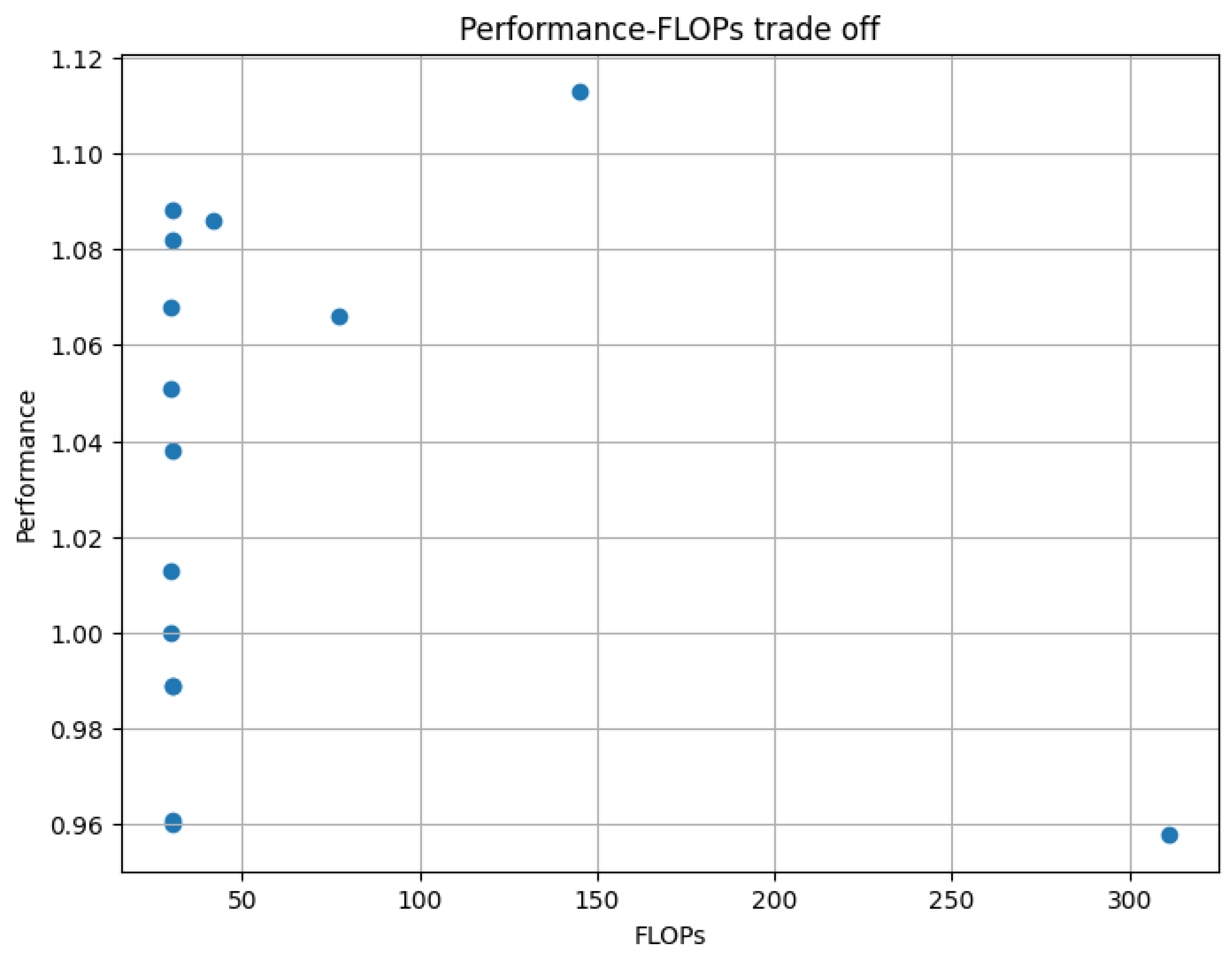
| Attention | Relative Performance | FLOPs (GFLOPS) | Params (K) |
|---|---|---|---|
| STDenseNet | 1.000 | 30.04 | 47.48 |
| MVSTGN | 0.416 | 33.72 | 284.19 |
| ADNet w. 3 × 3 Spatial | 1.013 | 30.06 | 47.52 |
| ADNet w. 5 × 5 Spatial | 1.051 | 30.10 | 47.59 |
| ADNet w. 7 × 7 Spatial | 1.038 | 30.17 | 47.68 |
| ADNet w. Channel | 0.961 | 30.13 | 48.72 |
| ADNet w. 3 × 3 CBAM | 0.989 | 30.15 | 52.44 |
| ADNet w. 5 × 5 CBAM | 0.989 | 30.19 | 52.70 |
| ADNet w. 7 × 7 CBAM | 0.960 | 30.25 | 53.08 |
| ADNet w. 3 × 3 Triplet | 1.068 | 30.10 | 47.61 |
| ADNet w. 5 × 5 Triplet | 1.088 | 30.20 | 47.80 |
| ADNet w. 7 × 7 Triplet | 1.082 | 30.34 | 48.09 |
| ADNet w. Non-local Softmax | 1.113 | 145.23 | 56.97 |
| ADNet w. Non-local Gaussian | 1.086 | 41.99 | 66.32 |
| ADNet w. Triplet Non-local Softmax | 0.958 | 311.13 | 97.67 |
| ADNet w. Triplet Non-local Gaussian | 1.066 | 77.02 | 147.32 |
| Position | Call | Internet | SMS |
|---|---|---|---|
| Before feature extraction | 13.86 (2.05) | 88.04 (14.23) | 26.28 (3.58) |
| Between feature extraction | 13.86 (1.76) | 94.22 (19.06) | 27.29 (3.07) |
| After feature extraction (ours) | 12.51 (1.75) | 84.31 (13.51) | 25.80 (2.42) |
Disclaimer/Publisher’s Note: The statements, opinions and data contained in all publications are solely those of the individual author(s) and contributor(s) and not of MDPI and/or the editor(s). MDPI and/or the editor(s) disclaim responsibility for any injury to people or property resulting from any ideas, methods, instructions or products referred to in the content. |
© 2025 by the authors. Licensee MDPI, Basel, Switzerland. This article is an open access article distributed under the terms and conditions of the Creative Commons Attribution (CC BY) license (https://creativecommons.org/licenses/by/4.0/).
Share and Cite
Oh, M.; Oh, S.; Im, J.; Kim, M.; Kim, J.-S.; Park, J.-Y.; Yi, N.-R.; Bae, S.-H. Comparative Analysis of Attention Mechanisms in Densely Connected Network for Network Traffic Prediction. Signals 2025, 6, 29. https://doi.org/10.3390/signals6020029
Oh M, Oh S, Im J, Kim M, Kim J-S, Park J-Y, Yi N-R, Bae S-H. Comparative Analysis of Attention Mechanisms in Densely Connected Network for Network Traffic Prediction. Signals. 2025; 6(2):29. https://doi.org/10.3390/signals6020029
Chicago/Turabian StyleOh, Myeongjun, Sung Oh, Jongkyung Im, Myungho Kim, Joung-Sik Kim, Ji-Yeon Park, Na-Rae Yi, and Sung-Ho Bae. 2025. "Comparative Analysis of Attention Mechanisms in Densely Connected Network for Network Traffic Prediction" Signals 6, no. 2: 29. https://doi.org/10.3390/signals6020029
APA StyleOh, M., Oh, S., Im, J., Kim, M., Kim, J.-S., Park, J.-Y., Yi, N.-R., & Bae, S.-H. (2025). Comparative Analysis of Attention Mechanisms in Densely Connected Network for Network Traffic Prediction. Signals, 6(2), 29. https://doi.org/10.3390/signals6020029