Article

Vector Signals and Invariant Systems: Re-Tooling Linear Systems Theory

by
Mamta Dalal
* and
Steven Sandoval
Klipsch School of Electrical and Computer Engineering, New Mexico State University, Las Cruces, NM 88003, USA
*
Author to whom correspondence should be addressed.
Signals 2025, 6(2), 28; https://doi.org/10.3390/signals6020028
Submission received: 11 April 2025 / Revised: 23 May 2025 / Accepted: 16 June 2025 / Published: 18 June 2025

Abstract

In a previous work, we identified the importance of rotation invariance in the standard complex-valued theory of linear time-invariant (LTI) systems and proposed a generalized vector-valued (VV) definition of convolution that reinterprets the complex-valued product of the traditional formalism as a scale rotation within the framework of geometric algebra. Based on this convolution definition, we characterized linear rotation-invariant time-invariant (LRITI) systems by defining and using a VV impulse response—effectively generalizing time-domain analysis for VV signals and LRITI systems. In this work, we provide a compatible frequency-domain analysis for VV signals and LRITI systems. First, VV bivector exponential signals are shown to be eigenfunctions of LRITI systems. A Fourier transform is defined, and we propose two generalized definitions of frequency response: the first valid for bivector exponentials in an arbitrary plane and the second valid for a general signal decomposed into a set of totally orthogonal planes (TOPs). Finally, we establish a convolution property for the Fourier transform with respect to TOPs. Together, these results provide compatible time-domain and frequency-domain analyses, thereby enabling a more comprehensive analysis of VV signals and LRITI systems.

1. Introduction

The study of linear time-invariant (LTI) systems plays an important role in various engineering fields [1,2]. The most commonly studied LTI systems are likely the complex-valued (CV) LTI systems, which enable a broad area of applications in signal analysis including filtering, system analysis, correlation, signal reconstruction, smoothing, compression, and time-frequency analysis, among others [3,4,5,6,7]. Within LTI systems analysis, convolution and the Fourier transform (FT) play important roles—convolution along with the impulse response helps to characterize LTI systems in the time domain, while the FT with the frequency response helps to characterize LTI systems in the frequency domain.
Several application-driven forms of extended or generalized convolution exist in the literature. A scalar convolution is defined on a vector field using the concept of the scalar product of two vectors [8]. A Clifford convolution, which is an extension of the scalar convolution, is studied in [9]. Several extensions of the convolution operation on multivector fields have been explored extensively [10,11,12]. A method for pattern matching on vector fields and vector filter masks using Clifford convolution is presented in [13].
Similarly, various application-driven extensions of FT have been proposed. The quaternion Fourier transform (QFT), which is one of the early extensions of the traditional FT, is proposed by Ell [14] for analyzing 2D-LTI systems and further studied by Bülow [15]. A hypercomplex extension to the standard complex Fourier transform is studied in [14], describing the quaternion Fourier transform as a double complex algebraic product. In [16], a hypercomplex Fourier transform is implemented by decomposition into two transforms that are isomorphic to the complex Fourier transform and provide a symplectic decomposition of the hypercomplex Fourier transform. Another quaternion Fourier transforms (QFT) is provided to study the analysis of higher-dimensional linear invariant systems in [17]. The spectral analysis of color images is studied using a generalized quaternion approach in [18]. In [19], a non-commutative multivector FT generalization of the QFT is studied. The Clifford FT for color images with a geometric approach using group action is given in [20]. In [21], the authors introduced a new equation within a Clifford algebra, whose solutions serve as kernels for a novel class of generalized Fourier transforms and are uniquely determined by a system of partial differential equations. A general geometric Fourier transform is defined for the multivector field over R p , q with values in GA, G p , q [22]. A generalization of the QFT to a general non-commutative Fourier transformation of functions from spacetime R 3 , 1 to the Clifford geometric algebra C l 3 , 1 is studied and used to further establish two multivector Fourier transforms in [19]. A detailed survey of the application of GA for image and signal processing is provided in [23].
The remainder of this paper is organized as follows. In Section 2, we discuss the traditional CV LTI systems theory, which we intend to generalize. In Section 3, we begin by introducing the notations and terminology we use for geometric algebra (GA). Following this, we present the essential tools to express the VV signals, emphasizing the polar representation and decomposition of VV signals. In Section 4, we present our extension of the traditional CV framework for LTI systems to a VV framework for linear rotation-invariant time-invariant (LRITI) systems, as proposed in [24]. This includes the definition of LRITI systems and VV convolution. Additionally, we provide a generalization of the commutative property for VV convolution. In Section 5, we provide our main contribution, that is, a frequency-domain analysis for VV signals that includes a Fourier transform (FT) for VV signals, the extension of the traditional frequency spectrum/response, and a convolution property for the FT. In Section 6, an example is provided to illustrate the usage of the proposed method. Finally, in Section 7 and Section 8, we discuss and conclude the article.

2. Traditional LTI Systems Theory

The typical theory of LTI systems allows for the analysis of signals, which are represented as time-series with complex values. These CV quantities are indicated using lowercase sans serif fonts, such as j , h , x , y , while the real-valued quantities are denoted using lowercase italic fonts, such as ω , t , τ , θ . Systems refer to mappings of signals and are denoted here using uppercase calligraphic letters, i.e., T , F . In the remainder of this section, we provide a summary of standard results that we intend to generalize. We omit the proofs; however, most of the standard results are provided in [1,2,25,26,27,28].
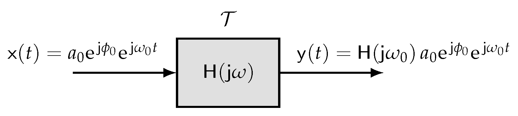
Definition 1 (Linear Systems). 
A CV system T is said to be linear if for an input consisting of a weighted sum of complex-valued signals, the output is a weighted sum of the system’s response to each of those signals
T k = 1 N a k x k ( t ) = k = 1 N a k T x k ( t )
where a k C .
Remark 1. 
In CV systems, rotation invariance (RI) naturally arises from the system’s linearity and by considering complex values as “scalars”. Consequently, a complex-valued system T is inherently rotation-invariant in the complex plane if it exhibits linearity
x ( t ) linearity k = 1 N x k ( t ) e j θ k T T y ( t ) linearity k = 1 N T x k ( t ) e j θ k .
Definition 2 (Time-Invariant Systems). 
A system T is said to be time-invariant (TI) if a time-shift in the input signal results in an identical time-shift in the output signal
T { x ( t t 0 ) } = y ( t t 0 ) .
Definition 3 (Sifting Property). 
The study of LTI systems in the time domain often begins with the representation of a signal in terms of a superposition of scaled shifted unit impulses
x ( t ) = x ( τ ) δ ( t τ ) d τ .
Definition 4 (Impulse Response). 
The impulse response of a system, T { · } , is the response of the system to a unit impulse (Dirac delta) applied at τ
h τ ( t ) = T δ ( t τ ) .
Corollary 1. 
If a system is time-invariant, then the response of that system to an impulse applied at an arbitrary time τ is equal to the response of the system to an impulse applied at the time τ = 0 , time-shifted by τ
h τ ( t ) = h 0 ( t τ ) .
Theorem 1 (The First Fundamental Theorem). 
Any LTI system T { · } can be completely characterized by a single signal called the system’s impulse response. Moreover, the output y ( t ) of an LTI system T { · } may then be expressed in terms of the convolution integral
y ( t ) = T { x ( t ) }
x ( t ) h ( t ) x ( τ ) h ( t τ ) d τ
and can be seen in the block diagram provided in Figure 1.
Theorem 2 (Commutative Property of CV Convolution). 
The CV convolution for LTI systems defined in (7b) is commutative
x ( t ) h ( t ) = h ( t ) x ( t )
x ( τ ) h ( t τ ) d τ = h ( τ ) x ( t τ ) d τ .
Remark 2. 
Careful inspection of (8b) reveals two important aspects: commutation of the product of the input signal and impulse response x ( · ) h ( · ) h ( · ) x ( · ) and the interchanging of the arguments of the input signal and impulse response ( τ ) ( t τ ) .
Definition 5 (Fourier Transform). 
The study of LTI systems in the frequency domain often begins with the definition of the Fourier transform. The Fourier transform of any signal x ( t ) is defined by
F x ( t ) x ( τ ) e j ω τ d τ .
Definition 6 (Complex Exponential Signals). 
A CT complex exponential signal is any CV signal which can be expressed as
x ( t ) = a 0 e j ϕ 0 e j ω 0 t
where a 0 R and ω 0 is the angular frequency.
Remark 3. 
The complex exponentials of different frequencies are orthogonal under the standard inner product defined on the space of square-integrable functions over an interval. In other words, their inner product is zero unless the frequencies are identical over a period.
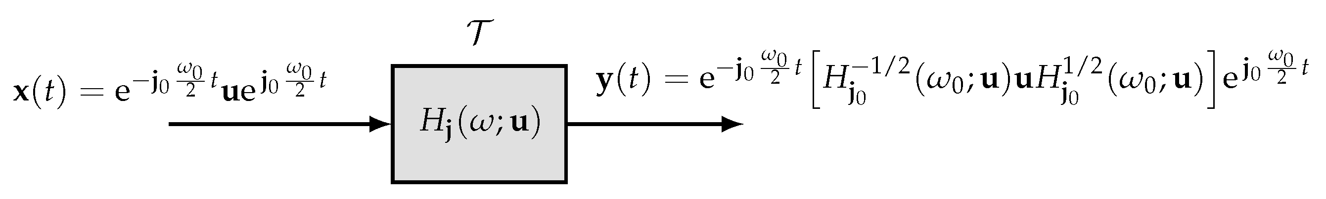
Definition 7 (Frequency Response). 
Any LTI system T { · } can be characterized in terms of a frequency response function as the FT of the impulse response
H ( j ω ) = F h ( t ) .
Definition 8 (Eigenfunction Property). 
The eigenfunction property of LTI systems is usually stated as follows. The response of an LTI system to a complex exponential input, a 0 e j ( ω 0 t + ϕ 0 ) , is
x ( t ) = a 0 e j ϕ 0 e j ω 0 t y ( t ) = H ( j ω 0 ) a 0 e j ϕ 0 e j ω 0 t
the same complex exponential with a multiplicative (scale-rotation) factor H ( j ω 0 ) —the eigenvalue associated with the complex exponential at frequency ω 0 . A block diagram representation for the same is provided in Figure 2.
Definition 9 (Frequency Spectrum). 
Any signal x ( t ) can be characterized in terms a frequency spectrum
X ( j ω ) = F x ( t ) .
Theorem 3 (Convolution Property of the FT). 
The Fourier transform of the convolution of two signals is equivalent to the product of their Fourier transforms
F { x ( t ) h ( t ) } = F { x ( t ) } F { h ( t ) } = X ( j ω ) H ( j ω ) .
Theorem 4 (The Second Fundamental Theorem). 
Any LTI system can be completely characterized by the system’s frequency response, which is defined as the Fourier transform of the system’s impulse response. Moreover, the spectrum of an LTI system’s output can be computed using the convolution property of the FT, by multiplying the input spectrum with the frequency response.

3. Notation and Terminology for Geometric Algebra

Although Clifford algebras may be defined over general fields, in GA, only real numbers are associated with scalar quantities, which are denoted using lowercase italic font, i.e., a , k , α , θ , t , τ R . Traditional (polar) vectors are associated with directed lengths and denoted using lowercase upright bold font, i.e., u , u , e 1 , x , y , h L n , where L n denotes the space of n-dimensional directed lengths. Traditional axial vectors are closely related with directed areas (bivectors) and denoted using uppercase upright bold font, i.e., B , B n where B n denotes the space of n-dimensional directed areas. The GA is a vector space with an additional product—the geometric product, which unifies the inner (dot) and exterior/outer (wedge) product between two vectors u , v into a single geometric product
u v = u · v + u v .
A summary of the properties of the dot, wedge, and geometric products is provided in Table 1.
For Euclidean spaces, the vector space L n can be extended to the geometric algebra G n . The canonical basis for G n is determined by an orthonormal basis for L n where the orthonormal basis vectors satisfy
e i e j = 1 , i = j e j e i , i j
where i , j = 1 , 2 , , N . The elements of G n are called multivectors and denoted by an uppercase italic font, i.e., X , R G n . One exception to the notational rules provided above is that simple unit bivectors j { B B n : B = 1 } are denoted with lowercase upright bold font j because they have the property
j 2 = 1 .
Furthermore, they play a role similar to that of the traditional imaginary number (as a generator of rotations). In a similar manner to how unit vectors are used to represent lines through the origin (where there are two unit vectors ± v corresponding to every line), unit bivectors may be used to represent planes through the origin. Thus, we will use the language “the plane j ” as an abbreviation for “the plane through the origin whose unit bivector is ± j ” [29].
A k-blade is any multivector that is expressible as the outer product of k linearly independent 1-vectors:
B = u 1 u 2 u k .
In G 3 , all non-zero k-vectors are k-blades. Let B = u 1 u 2 u k be a geometric product of orthogonal vectors. Then, the reverse of B is given as
B = u k u k 1 u 1 .
Suppose we have a vector a and a k-blade B . Then, the geometric product may be expressed as
a B = a · B + a B
where the inner (left contraction) and outer products are
a · B = a B k 1 , a B = a B 1 + k .
For additional details of GA theory, the reader is referred to the works of Macdonald [29,30,31], Hestenes [32,33], Doran et al. [34], and Riesz [35].
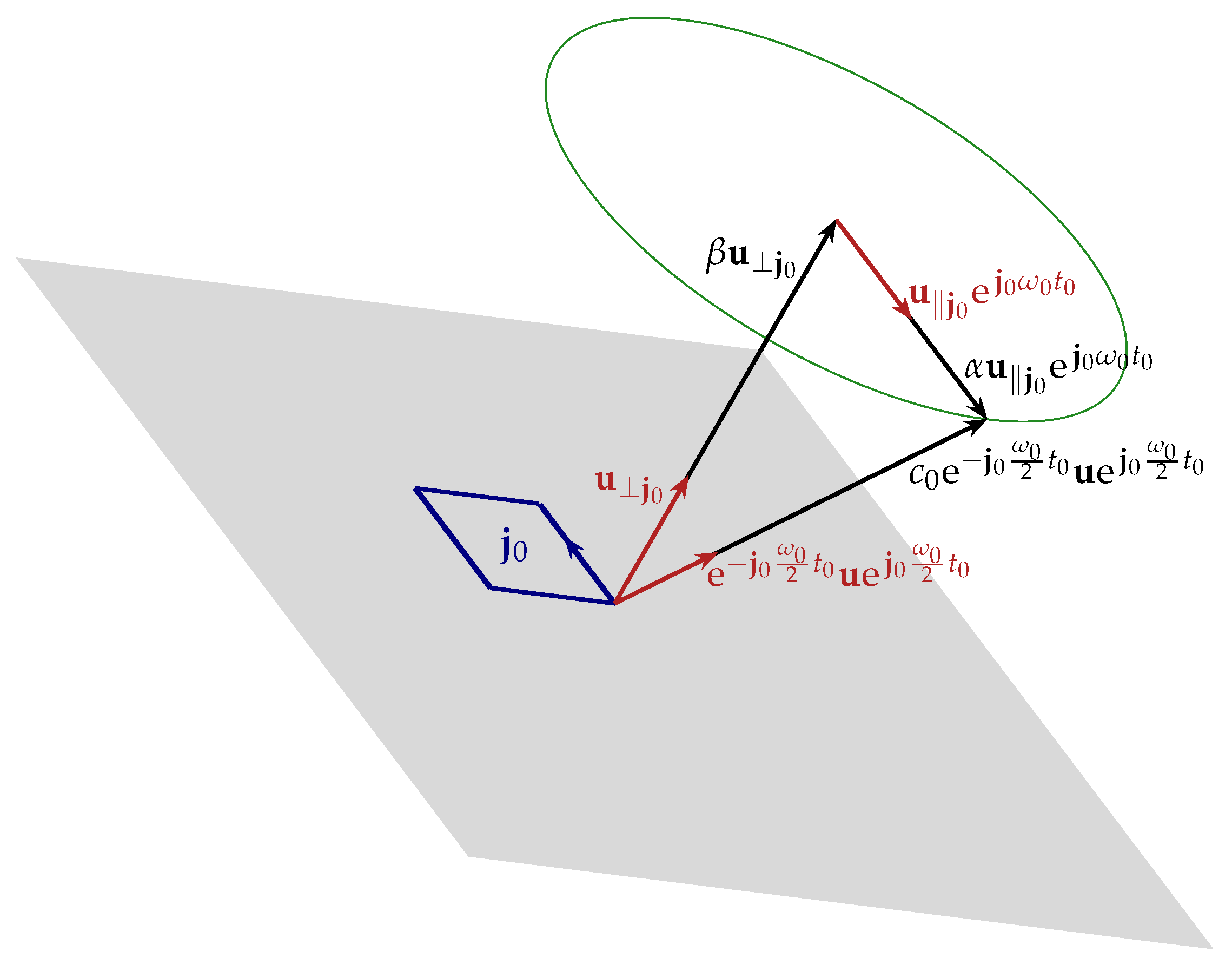
Definition 10 (Rotor). 
A rotor is a unit norm even grade multivector used to represent a rotation. A rotor R is any element of G n that can be written as the product of an even number of unit vectors and satisfies
R R = 1 .
Theorem 5 (Rotation of a Vector). 
Let u be a vector and R be a rotor; then, the rotation of vector u by R resulting in the vector u is expressed as
u = R 1 2 u R 1 2 .
Definition 11 (Simple Bivector). 
Let u and v be two orthogonal vectors; then, a simple bivector is defined as
u v = 1 2 ( u v v u ) = u v .
In Euclidean spaces, the square of a simple unit bivector j is j 2 = 1 .
Definition 12 (Simple Rotor). 
A rotor, R, that can be expressed as the product of two unit vectors, u , v , is called a simple rotor [33].
R = u v .
Any simple rotor R can be expressed in terms of the exponential of a simple bivector B
R = e B = e j θ .
Corollary 2 (Simple Rotation of a Vector). 
Let u denote the result of rotating the vector u in the plane j by angle θ. Then, u is expressed as
u = e j θ / 2 u e j θ / 2 .
Decomposing u in the plane j in (27) gives
u = e j θ / 2 u j + u j e j θ / 2
              = e j θ / 2 u j e j θ / 2 + e j θ / 2 u j e j θ / 2
= u j + u j e j θ .          
The result in (28c) illustrates how rotation affects the vector u within the plane of rotation j .
Remark 4. 
Let u denote the result of rotating the vector u in the plane j by angle θ. Then, the rotation of vector u performed from the right side is related to the rotation performed from the left side as
u = u e j θ = e j θ u .
Definition 13 (Polar Representation of a Vector-Valued Signal). 
We represent the VV signal x ( t ) L n t R in polar form relative to a Euclidean orthonormal basis vector e 1 as
x ( t ) = x ( t ) X 1 2 ( t ) e 1 X 1 2 ( t )
where x ( t ) is a real x ( t ) R t , and X ( t ) is a rotor formed as the sum of a scalar and bivector, i.e., { X R B n : X = 1 } .
Remark 5. 
For CV systems, there exists a distinguished axis (the real axis) that is used as the reference by which angles are measured. In other words, within the CV systems, the angle may be measured with respect to a unit element along the real axis in the complex plane. However, the proposed coordinate-free treatment of vector-valued systems has no such distinguished axis. Thus, we choose e 1 as our reference—essentially associating e 1 with the unit element along the real axis of the traditional CV linear systems theory.
Definition 14 (Totally Orthogonal Planes (TOPs)). 
Two planes j 1 and j 2 are totally orthogonal if they satisfy
j 1 j 2 = j 2 j 1 .
Corollary 3 (Commutative Rotations for TOPs). 
Let j 1 and j 2 be TOPs. Then, the associated rotations represented by the simple rotors R 1 = e j 1 θ 1 and R 2 = e j 2 θ 2 are commutative
R 1 1 2 R 2 1 2 u R 2 1 2 R 1 1 2 = R 2 1 2 R 1 1 2 u R 1 1 2 R 2 1 2 .
Definition 15 ((Canonical) Set of TOPs). 
We define a (canonical) set of totally orthogonal planes for N-dimensional space as
j k = e 2 k 1 e 2 k , k = 1 , 2 , , M
where M is given by
M = N 2 , N is even , N + 1 2 , N is odd .
For odd N-dimensional space, analysis is performed by embedding into an even N + 1 -dimensional space.
Remark 6. 
Embedding of an odd-dimensional space within an even-dimensional space may be considered as an extension of standard practice in the following sense. The analysis of a one-dimensional real-valued signal is conventionally performed by embedding the signal into the two-dimensional complex plane by considering it as a purely real CV signal.
Remark 7. 
TOPs have two important features: (1) They consist of pairwise commuting planes, which implies orthogonal (commuting) rotations [33]. This is important when considering rotations about arbitrary planes, because factoring a rotation into TOPs enables commutation of rotations in TOPs. (2) They form mutually exclusive or non-overlapping orthogonal planes in the sense that the intersection of the planes is empty. For example, in R 3 space, { e 1 e 2 , e 2 e 3 , e 3 e 1 } form a set of orthogonal planes. However, the planes e 1 e 2 and e 2 e 3 share any vector along the line of e 2 and the planes e 1 e 2 and e 3 e 1 share any vector along the line of e 1 . On the other hand, embedding R 3 into R 4 , we form the set of TOPs as { e 1 e 2 , e 3 e 4 } , which have no vectors in common. This is important when decomposing a signal into TOPs.
Definition 16 (Decomposition of a VV Signal into TOPs). 
A vector-valued signal x ( t ) in a finite N-dimensional space can always be decomposed into the projections with respect to the TOPs
x ( t ) = k = 1 M x j k ( t )
where j k is provided in (33) and M is given by (34).
Definition 17 (Polar Decomposition of a VV Signal Decomposed into TOPs). 
A vector-valued signal x ( t ) in N-dimensional space can always be decomposed in polar form relative to an Euclidean orthonormal basis vectors e 2 i 1 with M number of totally orthogonal planes
x ( t ) = i = 1 M x i ( t ) X i 1 2 ( t ) e 2 i 1 X i 1 2 ( t )
where M is given by (34).
Remark 8. 
In traditional LTI system theory, the real axis serves as a reference for measuring angles. To align with this convention, we adopt e 1 as the reference direction while using the polar decomposition of an arbitrary VV signal in (30). However, when we decompose the VV signal into TOPs, a reference vector (direction) must be specified for each TOP, as given in (36).

4. Time Domain Analysis for LRITI Systems

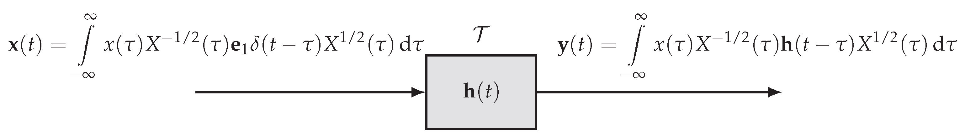
This section presents the relevant results from [24], where we introduced LRITI systems and defined a VV convolution. Traditionally, the CV convolution definition in (7) involves the product of two CV signals x ( t ) C t and h ( t ) C t , yielding a CV output signal y ( t ) C t . Direct extension of (7b) would imply the product of two VV signals x ( t ) L n t and h ( t ) L n t . However, this immediately contradicts the definition of a VV system, which has both a VV input and VV output, because the product of two VV signals is not a VV signal x ( t ) h ( t ) L n t . This leads to the reinterpretation of the CV product in CV convolution, allowing for a VV convolution in terms of a scale-rotation instead of a product.
In classical linear time-invariant (LTI) system theory, a single Dirac delta function—yielding a single impulse response—is typically sufficient to fully characterize the system’s behavior. However, in the context of vector-valued systems or those formulated within hypercomplex algebras, this assumption may no longer hold [17]. Preliminary insights suggest that at least two or more orthogonally directed, vector-valued impulse inputs are required to probe the system across independent orientations.
This limitation highlights the necessity of probing the system along multiple, independent input orientations to obtain a complete and informative response. This observation raises a fundamental and largely unexplored research question: What is the minimal and sufficient set of impulse responses required to uniquely characterize a vector-valued or hypercomplex-valued system? We give an answer in the context of LRITI systems that a single impulse response is sufficient to characterize a system. Additionally, a summary of the operators is provided in Table 2.

4.1. LRITI Systems

Definition 18 (Linear VV Systems). 
A system T is said to be linear if for an input consisting of a weighted sum of VV signals, the output is a weighted sum of the system’s response to each of those signals
T k = 1 N a k x k ( t ) = k = 1 N a k T x k ( t ) .
Remark 9. 
As previously noted, for CV systems, linearity in (1) implies rotational invariance as given in (2). However for VV systems, only real numbers are considered as “scalars”, and thus rotation invariance is not automatically inherited from (37) as it was from (1). Therefore, to maintain an alignment between the traditional and generalized theories, we define an additional property, termed rotational invariance.
Definition 19 (Rotation-Invariant VV Systems). 
A system T is said to be rotation-invariant if a rotation in the input signal results in an identical rotation in the output signal
x ( t ) rotate e j θ / 2 x ( t ) e j θ / 2 T T y ( t ) rotate e j θ / 2 T x ( t ) e j θ / 2 .
Definition 20 (Time-Invariant VV Systems). 
A system T is said to be a time-invariant if a time-shift in the input signal results in an identical time-shift in the output signal
T { x ( t t 0 ) } = y ( t t 0 ) .
Remark 10. 
The time-invariance property of the VV system (39) is a direct extension of the time-invariance property of the CV system (3).
Definition 21 (Sifting Property of Unit Impulse for VV Signals). 
Using the polar representation of a vector-valued signal in (30), we write the generalized sifting property of the unit impulse as
x ( t ) = x ( τ ) δ ( t τ ) d τ
          = x ( τ ) X 1 2 ( τ ) e 1 δ ( t τ ) X 1 2 ( τ ) d τ .
Remark 11. 
The expression in (40a) is a straightforward extension of (4), while (40b) provides the expression that enables us to leverage the rotation invariance (RI) property of LRITI systems.
Definition 22 (VV Impulse Response). 
We define the impulse response of a VV LRITI system due to an impulse at time t = τ in the e 1 direction as
h τ e 1 ( t ) T e 1 δ ( t τ ) .
For a time-invariant system, the response to an impulse at t = τ can be expressed in terms of the response to an impulse at t = 0 as
h τ e 1 ( t ) = h 0 e 1 ( t τ ) = h ( t τ ) .
For convenience, we usually drop the subscript and superscript.
Remark 12. 
The impulse response of the VV LRITI systems given in (41) and (42) are similar to CV LTI system (5) and (6), but additionally, a direction must be chosen in which to apply the impulse. We choose, for convention, the reference direction to be e 1 .
Theorem 6 (The First Fundamental Theorem). 
Any LRITI system T { · } can be completely characterized by the impulse response defined in (42). Moreover, the output y ( t ) of the LRITI system T { · } for arbitrary input x ( t ) represented in the polar form given in (30) can be computed with the convolution given by
y ( t ) = x ( t ) h ( t ) x ( τ ) X 1 2 ( τ ) h ( t τ ) X 1 2 ( τ ) d τ
The proof of the VV convolution (43) is provided in [24], and a block diagram representation is provided in Figure 3.
Remark 13. 
Since the traditional convolution definition (7b) is not directly applicable to vector-valued (VV) signals, we define a convolution operator specifically for VV signals (43). This definition leverages the rotation invariance (RI) property and represents the operation in terms of the scaling and rotation of the VV signal.
Remark 14. 
In traditional LTI systems theory, the commutative property of CV convolution given in (8b) enables us to derive the eigenfunction property of LTI systems given in (12). To proceed with a development of LRITI systems in a way that mirrors the traditional CV theory thus requires a generalization of (8). As noted in Remark 2, there are two important aspects to the commutative property of CV convolution (8b). Fortunately, derivation of the eigenfunction property of LRITI systems only requires the generalization of the second aspect. Therefore, to maintain an alignment between the traditional and generalized theories, we define an additional property to capture this second aspect, termed the flip-shift-slide property of VV Convolution.
Theorem 7 (Flip-Shift-Slide (FSS) Property of VV Convolution). 
The output of an LRITI system with a time-shift of the signal h ( t ) is equivalent to the output of the LRITI system with a time-shift of the input signal x ( t )
x ( τ ) X 1 2 ( τ ) h ( t τ ) X 1 2 ( τ ) d τ = x ( t τ ) X 1 2 ( t τ ) h ( τ ) X 1 2 ( t τ ) d τ .
The proof for the FSS property (44) is provided in Appendix A.1.

4.2. Summary of Time-Domain Analysis for VV Signals and LRITI Systems

In Section 4, we provided the properties of LRITI systems, including linearity, time invariance, and rotational invariance. Additionally, we introduced the sifting property of the Dirac delta and the impulse response for LRITI systems. We highlighted both the fundamental similarities and the distinctive differences of VV LRITI systems theory compared to traditional CV LTI systems theory. Furthermore, we pointed out that there are two aspects of the commutative property, and using the generalization of the second aspect is sufficient to derive the eigenfunction property of LRITI systems. Finally, we provide an answer to the open question posed by Ell in [17] regarding the number of impulse responses necessary to characterize a system. In particular, if the system is LRITI, then a single impulse response suffices. Furthermore, a key advantage of rotational invariance, in the context of the first fundamental theorem of the LRITI system, is that it simplifies system analysis in a manner similar to how time invariance benefits traditional LTI systems—–by reducing the number of impulse responses required for convolution.

5. Frequency Domain Analysis for LRITI Systems

As outlined in Section 1, numerous generalizations and modifications have been proposed to the conventional FT. However, for these FT generalizations, it is usually not clear how to define a compatible convolution definition for time-domain analysis (see pg. 10 in [17]). On the other hand, our approach has been to develop LRITI systems theory in a way that follows the same structure of mathematical arguments and logical reasoning as used with the development of traditional LTI systems theory. Explicitly, we started by defining a representation of a VV signal using scaled and shifted impulses and used it to develop a convolution that aligns and generalizes the traditional convolution. In the section that follows, we continue the development of LRITI systems theory in the frequency domain in a way that follows the same structure of mathematical arguments and logical reasoning as used with the development of traditional LTI systems theory, as closely as possible.
Definition 23 (Fourier Transform of a VV Signal). 
We define the FT of the VV signal x ( t ) with respect to arbitrary plane j as
F j { x ( t ) } e j ω 2 t x ( t ) e j ω 2 t d t .
Remark 15. 
The plane used in the traditional FT is always the complex plane j , but in (45), the plane j is an arbitrary unit bivector. Note that for L 2 space, the definition in (45) aligns with the traditional FT (9). See the proof in Appendix A.2.
Remark 16. 
The traditional FT for CV signals in (9) provides the weights of complex exponential signal components in the complex plane as a function of frequency, effectively providing a decomposition of the signal x ( t ) in terms of weighted complex exponential signal components. Unfortunately, while the FT for VV signals in (45) does provides the weights of bivector exponential signal components in the j 0 plane as a function of frequency, effectively providing a decomposition of the signal x j 0 ( t ) in terms of weighted bivector exponential signal components, the rejection x j 0 ( t ) from the plane j 0 is not appropriately accounted for.
Definition 24 (Accumulation).  
We define the accumulation operator Ac { · } as
Ac { x ( t ) } x ( t ) d t .
Definition 25 ((Vector-Valued) Bivector Exponential Signal). 
A (vector-valued) bivector exponential signal is any VV signal that may be expressed as
x ( t ) = c 0 e j 0 ω 0 2 t u e j 0 ω 0 2 t
    = c 0 e j 0 ω 0 2 t a 0 u j 0 + b 0 u j 0 e j 0 ω 0 2 t
  = c 0 e j 0 ω 0 2 t a 0 u j 0 e j 0 ω 0 2 t + c 0 e j 0 ω 0 2 t b 0 u j 0 e j 0 ω 0 2 t
  = ( c 0 a 0 ) u j 0 e j 0 ω 0 t + ( c 0 b 0 ) u j 0
    = α u j 0 e j 0 ω 0 t + β u j 0
where α = c 0 a 0 , β = c 0 b 0 , u j 0 is a unit vector that is rotated in the plane j 0 with constant amplitude α and constant angular velocity ω 0 and that is centered at β u j 0 , where u j 0 is a unit vector. An illustration of a bivector exponential signal is given in Figure 4.
Remark 17. 
For the complex exponential signal representation in (10), the complex plane j comprises the entire space under consideration. For the bivector exponential signal in (47e), the rotation occurs in the plane j 0 , but the space under consideration, L n , generally has dimension n different than two.
Remark 18. 
Unlike complex exponentials in Remark 3, bivector exponentials of different frequencies are not necessarily orthogonal because they may rotate in different planes. For bivector exponentials, orthogonality—as defined through rotations [33]—is not guaranteed.

5.1. Example 1 (Illustrating Non-Orthogonal Bivector Exponential via Rotations)

Suppose we are given two bivector exponential signals, denoted by x 1 ( t ) and x 2 ( t ) , each rotating in distinct planes with different angular frequencies ω 1 and ω 2 . Specifically, x 1 ( t ) rotates in the e 1 e 2 plane, while x 2 ( t ) rotates in the e 2 e 3 plane:
x 1 ( t ) = e 1 e j 1 ω 1 t , j 1 = e 1 e 2
x 2 ( t ) = e 2 e j 2 ω 2 t , j 2 = e 2 e 3 .
In GA, the orthogonality of the rotations is expressed by their commutativity [33]. Here, the rotations are defined by the bivector exponentials e j 1 ω 1 t and e j 2 ω 2 t . To determine whether the given rotations are orthogonal, we need to see whether the commutativity holds:
e j 1 ω 1 t e j 2 ω 2 t = e j 2 ω 2 t e j 1 ω 1 t .
To verify the commutativity in (49), we examine whether the bivectors j 1 and j 2 commute:
j 1 j 2 = ( e 1 e 2 ) ( e 2 e 3 )
= e 1 ( e 2 e 2 ) 1 e 3
= e 1 e 3    
j 2 j 1 = ( e 2 e 3 ) ( e 1 e 2 )
    = ( e 3 e 2 ) ( e 2 e 1 )
= e 3 ( e 2 e 2 ) 1 e 1
= e 3 e 1 .  
Clearly j 1 j 2 j 2 j 1 . Consequently, the bivector exponentials in (49) do not commute either, i.e., e j 1 ω 1 t e j 2 ω 2 t e j 2 ω 2 t e j 1 ω 1 t . Therefore, the rotations generated by these bivector exponentials are non-orthogonal.

5.2. Example 2 (Illustrating the Orthogonal Bivector Exponential via Rotations)

Suppose we are given two bivector exponential signals, denoted by x 1 ( t ) and x 2 ( t ) , each rotating in distinct planes with different angular frequencies ω 1 and ω 2 . Specifically, x 1 ( t ) rotates in the e 1 e 2 plane, while x 2 ( t ) rotates in the e 3 e 4 plane:
x 1 ( t ) = e 1 e j 1 ω 1 t , j 1 = e 1 e 2
x 2 ( t ) = e 3 e j 2 ω 2 t , j 2 = e 3 e 4 .
Similar to example 1, we just need to examine whether the bivectors j 1 and j 2 commute:
j 1 j 2 = ( e 1 e 2 ) ( e 3 e 4 )
= e 1 e 2 e 3 e 4
j 2 j 1 = ( e 3 e 4 ) ( e 1 e 2 )
= e 1 e 2 e 3 e 4 .
Clearly j 1 j 2 = j 2 j 1 . Consequently, the bivector exponentials commute, i.e., e j 1 ω 1 t e j 2 ω 2 t = e j 2 ω 2 t e j 1 ω 1 t . Therefore, the rotations generated by these bivector exponentials are orthogonal.
Examples 1 and 2 demonstrate that the orthogonality of bivector exponentials depends not only on their distinct angular frequencies but also on the planes in which the rotations occur.
Theorem 8 (Eigenfunctions of VV Convolution and LRITI Systems). 
Bivector exponential signals are eigenfunctions for VV convolution and LRITI systems.
Proof. 
Suppose the input to an LRITI system is the bivector exponential signal given in (47e). Then, using the VV convolution definition (43) gives
y ( t ) = x ( t ) h ( t )
= α u j 0 e j 0 ω 0 t + β u j 0 h ( t ) .
Using the polar representation gives
u j 0 = e 1 e j u ϕ , j u = e 1 u j 0 e 1 u j 0 , when e 1 u j 0 0 0 , otherwise
where ϕ is the angle between e 1 and u j 0 , and
u j 0 = e 1 e j v θ , j v = e 1 u e 1 u , when e 1 u 0 0 , otherwise
where θ is the angle between e 1 and u j 0 . Substitution of (54) and (55) in (53b) gives
y ( t ) = α e 1 e j u ϕ e j 0 ω 0 t + β e 1 e j v θ h ( t ) .
Using the FSS property (44) in (56) gives
y ( t ) = α e j 0 ω 0 2 ( t τ ) e j u ϕ 2 h ( τ ) e j u ϕ 2 e j 0 ω 0 2 ( t τ ) d τ + β e j v θ 2 h ( τ ) e j v θ 2 d τ
= α e j 0 ω 0 2 ( t τ ) e j u ϕ 2 h ( τ ) e j u ϕ 2 h R ( τ ) e j 0 ω 0 2 ( t τ ) d τ + β e j v θ 2 h ( τ ) e j v θ 2 d τ
= α e j 0 ω 0 2 ( t τ ) h R ( τ ) j 0 + h R ( τ ) j 0 e j 0 ω 0 2 ( t τ ) d τ + β e j v θ 2 h ( τ ) e j v θ 2 d τ
= α e j 0 ω 0 2 t e j 0 ω 0 2 τ h R ( τ ) j 0 e j 0 ω 0 2 τ d τ e j 0 ω 0 2 t + α e j 0 ω 0 2 t h R ( τ ) j 0 d τ e j 0 ω 0 2 t + β e j v θ 2 h ( τ ) d τ e j v θ 2
= α e j 0 ω 0 2 t e j 0 ω 0 2 τ h R ( τ ) j 0 e j 0 ω 0 2 τ d τ e j 0 ω 0 2 t + α h R ( τ ) j 0 d τ + β e j v θ 2 h ( τ ) d τ e j v θ 2
= [ α u j 0 e j 0 ω 0 t ] S j 0 ( ω 0 ) + α r ( j 0 ) + β e j v θ 2 a e j v θ 2
where we recognize that the spinor S j ( ω ) can be written in terms of the Fourier transform of the impulse response as
S j ( ω ) = u j 1 e j ω 2 τ e j u ϕ 2 h ( τ ) e j u ϕ 2 j e j ω 2 τ d τ u j 1 F j { ( e j u ϕ 2 h ( t ) e j u ϕ 2 ) j } ,
while the vector r ( j ) is the accumulation of the rejected part of the VV impulse response
r ( j ) = e j u ϕ 2 h ( τ ) e j u ϕ 2 j 0 d τ Ac e j u ϕ 2 h ( t ) e j u ϕ 2 j 0
and the vector a is the accumulation of the VV impulse response, h ( t ) ,
a = h ( τ ) d τ Ac { h ( t ) } .
Then, by defining
v j 0 = α u j 0 S j 0 ( ω 0 ) ,
and
v j 0 = α r ( j 0 ) + β e j v θ 2 a e j v θ 2 ,
we have
y ( t ) = v j 0 e j 0 ω 0 t + v j 0
= e j 0 ω 0 2 t v e j 0 ω 0 2 t .
Therefore, we have shown that bivector exponential signals are eigenfunctions of vector-valued convolution and LRITI systems. □
Definition 26 (Frequency Response). 
We define the frequency response as a spinor-valued function (proof is provided in Appendix A.4)
H j ( ω ; u ) u j ( α F j { ( e j u ϕ 2 h ( t ) e j u ϕ 2 ) j } + α Ac e j u ϕ 2 h ( t ) e j u ϕ 2 j + β e j v θ 2 Ac { h ( t ) } e j v θ 2 )
= u j α F j { e j u ϕ 2 h ( t ) e j u ϕ 2 } + β e j v θ 2 Ac { h ( t ) } e j v θ 2 .
In LTI system analysis, the frequency response is simply the FT of the impulse response (11), but with LRITI system analysis, the frequency response is seen as a spinor-valued function (64) and requires the FT of the scaled and rotated impulse response in an arbitrary plane j along with an additional accumulation term.
Corollary 4 (Eigenfunction Property). 
The response of an LRITI system to input x ( t ) = e j 0 ω 0 2 t u e j 0 ω 0 2 t may be expressed in terms of the frequency response as
y ( t ) = e j 0 ω 0 2 t H j 0 1 / 2 ( ω 0 ; u ) u H j 0 1 / 2 ( ω 0 ; u ) e j 0 ω 0 2 t .
A block diagram representation of the eigenfunction property is provided in Figure 5.
Remark 19. 
For L 2 space, the eigenfunction property (65) can be expressed as y ( t ) = u H j 0 ( ω 0 ; u ) e j 0 ω 0 t , which closely resembles the traditional eigenfunction property (12), except for the presence of the u term. This is because u , is in this case, is associated with the unit element in the complex plane. Regardless, the interpretation remains the same.

5.3. Synopsis

So far in Section 5, we developed frequency-domain analysis for VV LRITI systems and compared it with traditional CV LTI system theory. While the frequency response defined in (64) may be useful for bivector exponential signals, the utility for analysis on a general signal which has not been decomposed into bivector exponentials is not clear. This is because as noted in Remark 16 the FT we have defined in (45) does not provide a decomposition for a general VV signal. To address this challenge, we propose a decomposition approach based on the set of TOPs in (33), which provides an alternate approach to the frequency response of LRITI systems.
Definition 27 (Frequency Response with Respect to TOPs). 
The frequency response with respect to the TOPs is defined as
h ( t ) F j k { H j k ( ω ) }
where
H j k ( ω ) = F j k { h j k ( t ) } = h j k ( t ) e j k ω t d t .
The frequency response with respect to the TOPs (67) enables us to characterize the LRITI system by computing the FT of the projected impulse response in a finite number of planes, j k .
Definition 28 (Frequency Spectrum with Respect to TOP). 
The set of planar spectra for the signal x ( t ) is defined as
x ( t ) F j k { X j k ( ω ) }
where
X j k ( ω ) = F j k { x j k ( t ) } = x j k ( t ) e j k ω t d t .
A set of planar spectra, X j k ( ω ) , is introduced, which requires the FT of the signal projected in each of the TOPs’ planes (69), in contrast to the result in (45), which provides a single frequency spectrum for a given arbitrary plane, j .

5.4. Example 3 (Illustrating the Frequency-Domain Analysis Using TOPs in R 4 )

In this example, we will discuss the importance of TOPs to performing the frequency-domain analysis in a four-dimensional space. First, we will see why the FT in (45) is not sufficient to perform the frequency analysis, and then how TOPs enable the decomposition of the given signal and provide the FT of each of the decomposed signals in terms of their respective planar spectra, X j k ( ω ) .
We consider a four-dimensional space with the input signal x ( t ) given as
x ( t ) = e 1 e e 1 e 2 ω 0 t + e 4 cos ( ω 1 t ) .
Using the FT definition (45) for the given VV signal in (70) gives
F j { x ( t ) } = e j ω 2 t e 1 e e 1 e 2 ω 0 t + e 4 cos ( ω 1 t ) e j ω 2 t d t
= e j ω 2 t e 1 e e 1 e 2 ω 0 t e j ω 2 t d t I + e j ω 2 t e 4 cos ( ω 1 t ) e j ω 2 t d t II .
We observed, in (71b), that the term I consists of a VV signal rotating in the e 1 e 2 plane with angular frequency of ω 0 , while the term II contains a VV signal that oscillates with an angular frequency of ω 1 . To compute the FT of each of these terms requires the evaluation of their respective integrals. Without knowing the additional information about the arbitrary plane j , there are infinitely many choices in R 4 for us to consider in order to compute the FT of each of these terms. This limitation requires additional representation of the VV signal, which the proposed theory provides by decomposing the VV signal using TOPs.
Now, using the frequency spectrum in (69), which uses TOPs for the input signal in (70), gives
x ( t ) F j k { X j k ( ω ) } = { X j 1 ( ω ) , X j 2 ( ω ) }
= { e 1 2 π δ ( ω ω 0 ) , e 4 π δ ( ω ω 1 ) + π δ ( ω + ω 1 ) } .
In example 3, we discussed that the FT in (45) does not provide a decomposition for the given VV signal, x ( t ) . Thus, to perform the frequency-domain analysis for a given x ( t ) , we used a decomposition method utilizing a set of TOPs. We showed that the TOPs provided the frequency-domain analysis for the given VV signal in a finite number of planes, j k , and provided the FT of each decomposed signal in terms of their planar spectra, X j 1 ( ω ) , X j 2 ( ω ) , respectively.
Theorem 9 (Convolution Property of FT with respect to TOPs). 
The Fourier transform of the convolution of two VV signals is given by the following relation
F { x ( t ) h ( t ) } = k = 1 M F j k { h k ( t ) } e 2 k 1 F j k { x k ( t ) } + k = 1 M F j k { h k ( t ) } | k i | ( k i ) i = 1 M i k x i ( τ ) e j k ω τ d τ .
Additionally, in term of frequency spectrum, (73) can be written as
F { x ( t ) h ( t ) } = k = 1 M H j k ( ω ) e 2 k 1 X j k ( ω ) + k = 1 M H j k ( ω ) | k i | ( k i ) i = 1 M i k x i ( τ ) e j k ω τ d τ .
Proof. 
Operating the Fourier transform in (43) gives
F { y ( t ) } = F { x ( t ) h ( t ) }
Using the decomposition of the VV signal result (35) in (75) gives
F k = 1 M y j k ( t ) = F k = 1 M [ x ( t ) h ( t ) ] j k
= k = 1 M F [ x ( t ) h ( t ) ] j k
= k = 1 M e j k ω 2 t [ x ( t ) h ( t ) ] j k e j k ω 2 t d t .
Using the polar decomposition of VV signal x ( t ) with respect to the TOPs in (76c) gives
F k = 1 M [ x ( t ) h ( t ) ] j k = k = 1 M e j k ω 2 t i = 1 M x j i ( t ) h ( t ) j k e j k ω 2 t d t
Using the result for three-dimensional space where M = 2 gives (proof is provided in Appendix A.3)
F k = 1 2 [ x ( t ) h ( t ) ] j k = F j 1 { h 1 ( t ) } e 1 F j 1 { x 1 ( t ) } + F j 2 { h 2 ( t ) } e 3 F j 2 { x 2 ( t ) } + + F j 2 { h 2 ( t ) } x 1 ( τ ) e j 2 ω τ d τ j 2 + F j 1 { h 1 ( t ) } ( 1 ) x 2 ( τ ) e j 1 ω τ d τ j 1
Without loss of generality, we have
F { x ( t ) h ( t ) } = k = 1 M F j k { h k ( t ) } e 2 k 1 F j k { x k ( t ) } + k = 1 M F j k { h k ( t ) } | k i | ( k i ) i = 1 M i k x i ( τ ) e j k ω τ d τ .
Using the frequency spectrum result (69) in (79) gives
F { x ( t ) h ( t ) } = k = 1 M H j k ( ω ) e 2 k 1 X j k ( ω ) + k = 1 M H j k ( ω ) | k i | ( k i ) i = 1 M i k x i ( τ ) e j k ω τ d τ .
Theorem 10 (The Second Fundamental Theorem). 
The LRITI system in a given plane at a particular frequency is characterized by the system’s frequency response with respect to the TOP (67). Moreover, the spectrum of an LRITI system’s output can be computed using the convolution property of the FT with respect to TOPs (74).
Remark 20. 
For L 2 space, we have M = 1 , which further simplifies (74) and gives us F { x ( t ) h ( t ) } = H j 1 ( ω ) e 1 X j 1 ( ω ) , which aligns with the traditional convolution property (14) except for the presence of the e 1 term. This is because e 1 , in this case, is associated with the unit element in the complex plane.

5.5. Summary of Frequency-Domain Analysis for VV Signal and LRITI Systems

Section 5 presented the frequency-domain analysis, starting with the definition of the Fourier transform for VV signals and the bivector exponential signal, along with a comparison to traditional LTI system theory. We demonstrated that bivector exponential signals are eigenfunctions of VV convolution and LRITI systems. An important observation arises from the realization that, for VV LRITI systems, the traditional concepts of frequency response (11) and frequency spectrum (13) require significant modification to adequately perform frequency-domain analysis for a given arbitrary VV signal. This necessity leads us to reinterpret these concepts, resulting in two distinct definitions of frequency response. The first set of definitions, (64) and (45), establishes the frequency-domain analysis in a given arbitrary plane, j , which is proven to be sufficient for analyzing a bivector exponential signal (47a). On the other hand, the second set of definitions, (67) and (69), utilizes a decomposition method based on a set of TOPs (33), which is particularly useful for performing frequency-domain analysis for general VV signals. Finally, we provide a convolution property for the FT with respect to TOPs that unifies the time-domain and frequency-domain analysis for VV signals.

6. Example

In this example, we begin by analyzing an LRITI system in the time domain using the VV convolution definition in (43). Then, the same output is computed using the eigenfunction property in (65). Then, we analyze the LRITI system in the frequency domain using the Fourier transform in (45) and leveraging the set of TOPs in (33) to compute the frequency response of the LRITI system (67) and the frequency spectrum of the input signal (69). Regardless of the approach chosen, the same result is computed—thereby demonstrating that the proposed time-domain and frequency-domain analyses are consistent.
For the example, we consider a four-dimensional space with the input signal x ( t ) and impulse response h ( t ) , given as
x ( t ) = e 1 e e 1 e 2 ω 0 t + e 3 e e 3 e 4 ω 1 t ,
h ( t ) = ( e 1 + e 3 ) e α t u ( t ) , α > 0 .

6.1. Time-Domain Analysis Using Convolution Definition

Substituting (81a) and (81b) into the convolution definition (43) and using the FSS property (44) and (27) gives
y ( t ) = e e 1 e 2 ω 0 2 ( t τ ) e 1 e α τ u ( τ ) e e 1 e 2 ω 0 2 ( t τ ) d τ + e e 1 e 2 ω 0 2 ( t τ ) e 3 e α τ u ( τ ) e e 1 e 2 ω 0 2 ( t τ ) d τ + e e 3 e 4 ω 1 2 ( t τ ) e e 1 e 3 π 4 e 1 e α τ u ( τ ) e e 1 e 3 π 4 e e 3 e 4 ω 1 2 ( t τ ) d τ + e e 3 e 4 ω 1 2 ( t τ ) e e 1 e 3 π 4 e 3 e α τ u ( τ ) e e 1 e 3 π 4 e e 3 e 4 ω 1 2 ( t τ ) d τ
= e 1 ( α + e 1 e 2 ω 0 ) 1 e e 1 e 2 ω 0 t + e 3 1 α + e 3 ( α + e 3 e 4 ω 1 ) 1 e e 3 e 4 ω 1 t e 1 1 α .

6.2. Using Eigenfunction Property

The VV signal given in (81a) can be represented as
x ( t ) = e j 1 ω 0 2 t e 1 e j 1 ω 0 2 t + e j 2 ω 1 2 t e 3 e j 2 ω 1 2 t
= e j 1 ω 0 2 t u 1 e j 1 ω 0 2 t + e j 2 ω 1 2 t u 2 e j 2 ω 1 2 t
and using the eigenfunction property (65) gives
y ( t ) = e j 1 ω 0 2 t H j 1 1 / 2 ( ω 0 ; u 1 ) u 1 H j 1 1 / 2 ( ω 0 ; u 1 ) e j 1 ω 0 2 t + e j 2 ω 1 2 t H j 2 1 / 2 ( ω 1 ; u 2 ) u 2 H j 2 1 / 2 ( ω 1 ; u 2 ) e j 2 ω 1 2 t
= e j 1 ω 0 2 t u 1 H j 1 ( ω 0 ; u 1 ) e j 1 ω 0 2 t + e j 2 ω 1 2 t u 2 H j 2 ( ω 1 ; u 2 ) e j 2 ω 1 2 t .
The frequency response in (64a) with α = 1 , β = 0 gives
H j 1 ( ω ; u 1 ) u 1 j 1 ( F j 1 { ( e j u ϕ 2 h ( t ) e j u ϕ 2 ) j 1 } + Ac e j u ϕ 2 h ( t ) e j u ϕ 2 j 1
where j u = 0 , which further simplifies (85) and gives
H j 1 ( ω ; u 1 ) u 1 j 1 ( F j 1 { h ( t ) j 1 } + Ac h ( t ) j 1
= e 1 e 1 ( α + e 1 e 2 ω ) 1 + e 3 e α t u ( t ) d τ
    = e 1 e 1 ( α + e 1 e 2 ω ) 1 + e 3 1 α
    = ( α + e 1 e 2 ω ) 1 + e 1 e 3 1 α
H j 1 ( ω 0 ; u 1 ) = ( α + e 1 e 2 ω 0 ) 1 + e 1 e 3 1 α .        
Similarly, we have
H j 2 ( ω ; u 2 ) u 2 j 2 ( F j 2 { ( e j u ϕ 2 h ( t ) e j u ϕ 2 ) j 2 } + Ac e j u ϕ 2 h ( t ) e j u ϕ 2 j 2
where j u = e 1 e 3 and ϕ = π 2 , which further simplifies (87) and gives
H j 2 ( ω ; u 2 ) u 2 j 2 ( F j 2 { ( e e 1 e 3 π 4 h ( t ) e e 1 e 3 π 4 ) j 2 } + Ac e e 1 e 3 π 4 h ( t ) e e 1 e 3 π 4 j 2
= e 3 e 3 ( α + e 3 e 4 ω ) 1 + e 1 e α t u ( t ) d τ    
= e 3 e 3 ( α + e 3 e 4 ω ) 1 e 1 1 α    
= ( α + e 3 e 4 ω ) 1 e 3 e 1 1 α    
H j 2 ( ω 1 ; u 2 ) = ( α + e 3 e 4 ω 1 ) 1 e 3 e 1 1 α .
Substituting H j 1 ( ω 0 ; u 1 ) from (86e) and H j 2 ( ω 1 ; u 2 ) from (88e) into (84b) gives
y ( t ) = e j 1 ω 0 2 t e 1 ( α + e 1 e 2 ω 0 ) 1 + e 1 e 3 1 α e j 1 ω 0 2 t + e j 2 ω 1 2 t e 3 ( α + e 3 e 4 ω 1 ) 1 e 3 e 1 1 α e j 2 ω 1 2 t
    = e 1 ( α + e 1 e 2 ω 0 ) 1 e e 1 e 2 ω 0 t + e 3 1 α + e 3 ( α + e 3 e 4 ω 1 ) 1 e e 3 e 4 ω 1 t e 1 1 α .

6.3. Frequency-Domain Analysis Using FT for Given VV Signals

Using the frequency spectrum in (69) for the output signal in (82b),
y ( t ) F j k { Y j k ( ω ) } = { Y j 1 ( ω ) , Y j 2 ( ω ) }
  = { e 1 ( α + e 1 e 2 ω 0 ) 1 2 π δ ( ω ω 0 ) e 1 1 α 2 π δ ( ω ) , e 3 1 α 2 π δ ( ω ) + e 3 ( α + e 3 e 4 ω 1 ) 1 2 π δ ( ω ω 1 ) } .

6.4. Using Convolution Property of FT for the Given VV Signals

Using the frequency response in (67) for the impulse response in (81b),
h ( t ) F j k { H j k ( ω ) } = { H j 1 ( ω ) , H j 2 ( ω ) }
= { e 1 ( α + e 1 e 2 ω ) 1 , e 3 ( α + e 3 e 4 ω ) 1 } ,
and using the frequency spectrum in (69) for the input signal in (81a)
x ( t ) F j k { X j k ( ω ) } = { X j 1 ( ω ) , X j 2 ( ω ) }
= { e 1 2 π δ ( ω ω 0 ) , e 4 2 π δ ( ω ω 1 ) } .
Using the convolution property of the FT given in (73) gives
F { x ( t ) h ( t ) } = F j 1 { h 1 ( t ) } e 1 F j 1 { x 1 ( t ) } + F j 2 { h 2 ( t ) } x 1 ( τ ) e j 2 ω τ d τ + F j 2 { h 2 ( t ) } e 3 F j 2 { x 2 ( t ) } + F j 1 { h 1 ( t ) } ( 1 ) x 2 ( τ ) e j 1 ω τ d τ
  = e 1 ( α + j 1 ω 0 ) 1 2 π δ ( ω ω 0 ) + e 3 ( α + j 2 ω 1 ) 1 2 π δ ( ω ) + e 3 ( α + j 2 ω 1 ) 1 2 π δ ( ω ω 1 ) e 1 ( α + j 1 ω 0 ) 1 2 π δ ( ω ) .
Then, using the sampling property of the Dirac delta gives
F { x ( t ) h ( t ) } = e 1 ( α + j 1 ω 0 ) 1 2 π δ ( ω ω 0 ) + e 3 ( α + j 2 ( 0 ) ) 1 2 π δ ( ω ) + e 3 ( α + j 2 ω 1 ) 1 2 π δ ( ω ω 1 ) e 1 ( α + j 1 ( 0 ) ) 1 2 π δ ( ω )
    = e 1 ( α + j 1 ω 0 ) 1 2 π δ ( ω ω 0 ) + e 3 1 α 2 π δ ( ω ) + e 3 ( α + j 2 ω 1 ) 1 2 π δ ( ω ω 1 ) e 1 1 α 2 π δ ( ω ) .
Finally, for comparison, the terms given in (94b) are partitioned into the set of TOPs as
F { x ( t ) h ( t ) } = { e 1 ( α + e 1 e 2 ω 0 ) 1 2 π δ ( ω ω 0 ) e 1 1 α 2 π δ ( ω ) , e 3 1 α 2 π δ ( ω ) + e 3 ( α + e 3 e 4 ω 1 ) 1 2 π δ ( ω ω 1 ) } .

6.5. Example Summary

The proposed methodology can be observed to be self-consistent for the example as follows. The output signal using VV convolution in (82b) matches with (89b), which utilizes the eigenfunction property. Additionally, the FT of the output signal using VV convolution in (90b) matches with (95), which utilizes the convolution property of the FT.

7. Discussion

The main goal of this work was to develop a time-domain and frequency-domain analyses for VV signals and LRITI systems which aligns with the traditional theory for CV signals and LTI systems. In the transition from the CV theory, where scalars are complex-valued, to the VV theory where scalars are considered real-valued, the linearity property suffered a loss of rotational invariance. Thus, to define a VV theory which aligns with the CV theory, required the specification of a rotational invariance property in addition to linearity for VV systems.
Using the polar representation of the VV signal in (30) allowed us to define the sifting property for VV signals in (40b) which we leverage along with the properties of linearity (L), rotation invariance (RI), and time invariance (TI) leading to a definition of VV convolution. With VV convolution defined, the bivector exponential signals are shown to be eigenfunction of convolution and LRITI systems. A frequency response is defined which further demonstrates that bivector exponentials take the place of complex exponentials in the traditional theory.
While the frequency response in (64) allows the output of an LRITI system to be computed for an input consisting of an arbitrary bivector exponential, the FT in (45) does not provide a decomposition for an arbitrary input signal. Thus, to perform the frequency-domain analysis for a general VV signal, we introduce a decomposition method utilizing a set of TOPs. Leveraging the TOPs, we define a frequency spectrum for VV signals in (69) and a frequency response for LRITI sytems in (67) which aligns with and generalizes the frequency spectrum and frequency response of CV theory. Finally, the convolution property of the FT for VV signals is derived which generalizes the results from CV theory.
While extending the theory of CV signals and LTI systems to the theory for VV signals and LRITI systems, there were two instances where a traditional property pulled apart into two distinct pieces. First, the linearity property of the traditional CV LTI system theory, which inherently implies the rotation-invariance (RI) property for CV signals, (complex) linearity separates into two distinct concepts: (real) linearity and rotation-invariance (RI). Second, the commutative property of VV convolution requires the separation of two concepts in the definition of convolution: commutative multiplication of the input signal and impulse response and the swapping/interchanging of the arguments of the input signal and the impulse response. Additionally, a comparative summary of the notations and definitions used for traditional CV signals and VV signals is provided in Table 3. Another comparative study of the traditional CV thoery and the proposed VV theory is provided in Table 4.
One significant difference between CV and VV theory is that the Fourier transform (FT) does not enable decomposition in a space with dimensions higher than a plane. This is because in traditional CV theory, frequency-domain analysis relies on the complex plane, which intrinsically supports only two-dimensional signal representations. For vector-valued signals in R N , with N > 2 , this limitation necessitates a channel-wise decomposition—treating each component separately using complex planes resulting in N scalar complex computations. This approach loses the geometric relationships among components and fails to provide a unified spectral interpretation in arbitrary dimensions.
For N > 2 , a vector-valued signal cannot be naturally decomposed within the complex plane, as complex numbers inherently represent only two-dimensional structures. This motivates the need for more general algebraic frameworks—such as geometric algebra—that can represent and manipulate an arbitrary-dimensional VV signals in a unified and coordinate-free manner.
Therefore, we propose to resolve the issue by use of TOPs. For an arbitrary dimension, N TOPs decomposition provides a principled approach in representing VV signals in a set of mutually orthogonal planes. This framework enables a unified and geometrically meaningful analysis of signals across arbitrary dimensions. TOPs provide frequency-domain analysis for a general VV signal in a finite number of planes, j k . TOPs enables one to compute the FT of each decomposed signal in terms of planar spectra, X j k ( ω ) , in their respective planes.
To generalize the frequency-domain analysis, we introduced two distinct definitions of the frequency response: a first that is valid for a bivector exponential signal in an arbitrary plane and a second that is valid for a general VV signal decomposed into a set of TOPs. While we can define two different frequency responses, the one which does not use TOPs is of limited utility, because of the lack of a decomposition algorithm.
Additionally, an advantage of the partitioning of a signal into TOPs lies in the fact that standard CV theory is essentially a “planar theory”. Thus, by partitioning the analysis into TOPs, we can leverage much of our existing knowledge and expertise.

8. Conclusions

Geometric algebra provides a power set of mathematical tools for carrying out coordinate-free signal processing. Unfortunately, it is not obvious how to extend many of the most commonly used tools in signal processing (such as convolution and frequency response) from operations defined on complex-valued (CV) time-series in C , to operations defined on vector-valued (VV) times-series in L n . Moreover, a proper holistic extension of the conventional theory could lead to a deeper understanding of multidimensional signal analysis and potentially unlock more efficient computational methods for image and signal processing.
To that end, we have proposed a set of definitions of convolution, Fourier transform (FT), frequency response, and frequency spectrum for VV signals and linear rotation-invariant time-invariant (LRITI) systems, which closely aligns and generalizes the theory for CV signals and linear time-invariant (LTI) systems. However, we provide a frequency response that is valid in the context of bivector exponential signals; the lack of a matching decomposition algorithm for a general VV signal prevents further utility. This leads to the definition of both a frequency spectrum and frequency response with respect to a set of totally orthogonal planes (TOPs). Finally, the convolution property of the FT for VV signals is derived, establishing a relationship between time-domain and frequency-domain analysis, which we believe aligns as closely as possible with the CV LTI system theory.

Author Contributions

Conceptualization, M.D. and S.S.; methodology, M.D. and S.S.; software, S.S.; validation, M.D. and S.S.; formal analysis, M.D. and S.S.; investigation, M.D.; resources, M.D.; writing—original draft, M.D. and S.S.; writing—review and editing, M.D. and S.S.; visualization, S.S.; supervision, S.S.; project administration, S.S. All authors have read and agreed to the published version of the manuscript.

Funding

This research received no external funding.

Data Availability Statement

No new data were created or analyzed in this study. Data sharing is not applicable to this article.

Conflicts of Interest

The authors declare no conflicts of interest.

Appendix A. Supporting Proofs

Appendix A.1. Flip Shift Slide Property Proof

Proof. 
Substitution of variables as t τ = u τ = t u and d τ = d u into (43) gives
y ( t ) = x ( t u ) X 1 / 2 ( t u ) h ( u ) X 1 / 2 ( t u ) d u .
Again, replacing the variable u in (A1) by an arbitrary variable τ gives
y ( t ) = x ( t τ ) X 1 / 2 ( t τ ) h ( τ ) X 1 / 2 ( t τ ) d τ .

Appendix A.2. For N = 2, Proposed FT Reduces to the Traditional FT Proof

Proof. 
Suppose in two-dimensional Euclidean space, an input signal x ( t ) L 2 to an LRITI system is given by (47a). The Fourier transform of the VV signal x ( t ) is given by substituting (47a) into (45), which gives
F j { x ( t ) } = e j ω 2 t c 0 e j 0 ω 0 2 t u e j 0 ω 0 2 t e j ω 2 t d t .
This is because in L 2 space, we have j = j 0 , which further simplifies (A3) and gives
F j 0 { x ( t ) } = e j 0 ω 2 t c 0 e j 0 ω 0 2 t u e j 0 ω 0 2 t e j 0 ω 2 t d t
= c 0 e j 0 ω 2 t e j 0 ω 0 2 t u e j 0 ω 0 2 t e j 0 ω 2 t d t
= c 0 e j 0 ( ω ω 0 2 ) t u e j 0 ( ω ω 0 2 ) t d t
= c 0 u e j 0 ( ω ω 0 ) t d t
= c 0 u 2 π δ ( ω ω 0 ) .
Thus, we observed that the Fourier transform of the VV bivector exponential signal in lower dimension ( L 2 ) agrees with the conventional complex Fourier transform where j 0 plays the role of the complex plane, j . □

Appendix A.3. Convolution Property of FT for a 3-Dimensional Space Proof

Proof. 
For three-dimensional space, using M = 2 in (77) gives
F k = 1 2 [ x ( t ) h ( t ) ] j k = k = 1 2 e j k ω 2 t i = 1 2 x j i ( t ) h ( t ) j k e j k ω 2 t d t .
Using the polar decomposition of VV signal x ( t ) with respect to the totally orthogonal planes (TOP) M = 2 in (A5) gives
i = 1 2 x j i ( t ) = i = 1 2 ( e 2 i 1 ) 2 x j i ( t )
= ( e 1 ) 2 x j 1 ( t ) + ( e 3 ) 2 x j 2 ( t )
= e 1 ( e 1 x j 1 ( t ) ) + e 3 ( e 3 x j 2 ( t ) )
= e 1 ( x 1 ( t ) X 1 ( t ) ) + e 3 ( x 2 ( t ) X 2 ( t ) )
= x 1 ( t ) [ e 1 X 1 ( t ) ] + x 2 ( t ) [ e 3 X 2 ( t ) ]
= x 1 ( t ) [ e 1 X 1 ( t ) ] + x 2 ( t ) [ e 1 X 1 ( t ) R ( t ) ] , R ( t ) = X 1 1 ( t ) e e 1 e 3 π 2 X 2 ( t )
= x 1 ( t ) X 1 1 / 2 ( t ) e 1 X 1 1 / 2 ( t ) + x 2 ( t ) R 1 / 2 ( t ) X 1 1 / 2 ( t ) e 1 X 1 1 / 2 ( t ) R 1 / 2 ( t ) .
Using (A6g) in (A5) gives
F k = 1 2 [ x ( t ) h ( t ) ] j k = k = 1 2 e j k ω 2 t [ ( x 1 ( t ) X 1 1 / 2 ( t ) e 1 X 1 1 / 2 ( t ) + x 2 ( t ) R 1 / 2 ( t ) X 1 1 / 2 ( t ) e 1 X 1 1 / 2 ( t ) R 1 / 2 ( t ) ) h ( t ) ] j k e j k ω 2 t d t
= k = 1 2 e j k ω 2 t x 1 ( t ) X 1 1 / 2 ( t ) e 1 X 1 1 / 2 ( t ) h ( t ) j k e j k ω 2 t d t + k = 1 2 e j k ω 2 t [ ( x 2 ( t ) R 1 / 2 ( t ) X 1 1 / 2 ( t ) e 1 X 1 1 / 2 ( t ) R 1 / 2 ( t ) ) h ( t ) ] j k e j k ω 2 t d t
= k = 1 2 e j k ω 2 t [ x 1 ( τ ) X 1 1 / 2 ( τ ) h ( t τ ) X 1 1 / 2 ( τ ) d τ ] j k e j k ω 2 t d t + k = 1 2 e j k ω 2 t [ x 2 ( τ ) R 1 / 2 ( τ ) X 1 1 / 2 ( τ ) h ( t τ ) X 1 1 / 2 ( τ ) R 1 / 2 ( τ ) d τ ] j k e j k ω 2 t d t .
Using substitution of the variables, we can write
t τ = u d t = d u
t = u + τ .
Substituting (A8) and (A9) into (A7c) gives
F k = 1 2 [ x ( t ) h ( t ) ] j k = k = 1 2 e j k ω 2 ( u + τ ) x 1 ( τ ) X 1 1 / 2 ( τ ) h ( u ) X 1 1 / 2 ( τ ) d τ j k e j k ω 2 ( u + τ ) d u + k = 1 M e j k ω 2 ( u + τ ) [ x 2 ( τ ) R 1 / 2 ( τ ) X 1 1 / 2 ( τ ) h ( u ) X 1 1 / 2 ( τ ) R 1 / 2 ( τ ) d τ ] j k e j k ω 2 ( u + τ ) d u .
Now, using the polar decomposition of VV signal h ( u ) with respect to the totally orthogonal planes (TOP) with M = 2 gives
j = 1 2 h j j ( t ) = i = 1 2 ( e 2 i 1 ) 2 h j j ( u )
  = ( e 1 ) 2 h j 1 ( u ) + ( e 3 ) 2 h j 2 ( u )
  = e 1 ( e 1 h j 1 ( u ) ) + e 3 ( e 3 h j 2 ( u ) )
    = e 1 ( h 1 ( u ) H 1 ( u ) ) + e 3 ( h 2 ( u ) H 2 ( u ) ) .
Substituting (A11d) in (A10) gives
F k = 1 2 [ x ( t ) h ( t ) ] j k = k = 1 2 e j k ω 2 ( u + τ ) [ x 1 ( τ ) X 1 1 / 2 ( τ ) ( h 1 ( u ) e 1 H 1 ( u ) + h 2 ( u ) e 3 H 2 ( u ) ) X 1 1 / 2 ( τ ) d τ ] j k e j k ω 2 ( u + τ ) d u + k = 1 2 e j k ω 2 ( u + τ ) [ x 2 ( τ ) R 1 / 2 ( τ ) X 1 1 / 2 ( τ ) h 1 ( u ) e 1 H 1 ( u ) + h 2 ( u ) e 3 H 2 ( u ) X 1 1 / 2 ( τ ) R 1 / 2 ( τ ) d τ ] j k e j k ω 2 ( u + τ ) d u
= k = 1 M e j k ω 2 ( u + τ ) [ x 1 ( τ ) X 1 1 / 2 ( τ ) h 1 ( u ) e 1 H 1 ( u ) X 1 1 / 2 ( τ ) d τ ] j k e j k ω 2 ( u + τ ) d u + k = 1 2 e j k ω 2 ( u + τ ) [ x 1 ( τ ) X 1 1 / 2 ( τ ) h 2 ( u ) e 3 H 2 ( u ) X 1 1 / 2 ( τ ) d τ ] j k e j k ω 2 ( u + τ ) d u + k = 1 2 e j k ω 2 ( u + τ ) [ x 2 ( τ ) R 1 / 2 ( τ ) X 1 1 / 2 ( τ ) h 1 ( u ) e 1 H 1 ( u ) X 1 1 / 2 ( τ ) R 1 / 2 ( τ ) d τ ] j k e j k ω 2 ( u + τ ) d u + k = 1 2 e j k ω 2 ( u + τ ) [ x 2 ( τ ) R 1 / 2 ( τ ) X 1 1 / 2 ( τ ) h 2 ( u ) e 3 H 2 ( u ) X 1 1 / 2 ( τ ) R 1 / 2 ( τ ) d τ ] j k e j k ω 2 ( u + τ ) d u .
Further simplification leads to
F k = 1 2 [ x ( t ) h ( t ) ] j k = e j 1 ω 2 ( u + τ ) [ x 1 ( τ ) X 1 1 / 2 ( τ ) h 1 ( u ) e 1 H 1 ( u ) X 1 1 / 2 ( τ ) d τ ] j 1 e j 1 ω 2 ( u + τ ) d u + e j 2 ω 2 ( u + τ ) [ x 1 ( τ ) X 1 1 / 2 ( τ ) h 1 ( u ) e 1 H 1 ( u ) X 1 1 / 2 ( τ ) d τ ] j 2 e j 2 ω 2 ( u + τ ) d u + e j 1 ω 2 ( u + τ ) [ x 1 ( τ ) X 1 1 / 2 ( τ ) h 2 ( u ) e 3 H 2 ( u ) X 1 1 / 2 ( τ ) d τ ] j 1 e j 1 ω 2 ( u + τ ) d u + e j 2 ω 2 ( u + τ ) [ x 1 ( τ ) X 1 1 / 2 ( τ ) h 2 ( u ) e 3 H 2 ( u ) X 1 1 / 2 ( τ ) d τ ] j 2 e j 2 ω 2 ( u + τ ) d u + e j 1 ω 2 ( u + τ ) [ x 2 ( τ ) R 1 / 2 ( τ ) X 1 1 / 2 ( τ ) h 1 ( u ) e 1 H 1 ( u ) X 1 1 / 2 ( τ ) R 1 / 2 ( τ ) d τ ] j 1 e j 1 ω 2 ( u + τ ) d u + e j 2 ω 2 ( u + τ ) [ x 2 ( τ ) R 1 / 2 ( τ ) X 1 1 / 2 ( τ ) h 1 ( u ) e 1 H 1 ( u ) X 1 1 / 2 ( τ ) R 1 / 2 ( τ ) d τ ] j 2 e j 2 ω 2 ( u + τ ) d u + e j 1 ω 2 ( u + τ ) [ x 2 ( τ ) R 1 / 2 ( τ ) X 1 1 / 2 ( τ ) h 2 ( u ) e 3 H 2 ( u ) X 1 1 / 2 ( τ ) R 1 / 2 ( τ ) d τ ] j 1 e j 1 ω 2 ( u + τ ) d u + e j 2 ω 2 ( u + τ ) [ x 2 ( τ ) R 1 / 2 ( τ ) X 1 1 / 2 ( τ ) h 2 ( u ) e 3 H 2 ( u ) X 1 1 / 2 ( τ ) R 1 / 2 ( τ ) d τ ] j 2 e j 2 ω 2 ( u + τ ) d u .
Collecting the non-zero terms gives us
F k = 1 2 [ x ( t ) h ( t ) ] j k = e j 1 ω 2 τ x 1 ( τ ) X 1 1 / 2 ( τ ) F j 1 { h 1 ( t ) } X 1 1 / 2 ( τ ) j 1 e j 1 ω 2 τ d τ + e j 2 ω 2 τ x 1 ( τ ) F j 2 { h 2 ( t ) } j 2 e j 2 ω 2 τ d τ + e j 2 ω 2 τ x 2 ( τ ) X 2 1 / 2 ( τ ) F j 2 { h 2 ( t ) } X 2 1 / 2 ( τ ) j 2 e j 2 ω 2 τ d τ e j 1 ω 2 τ x 2 ( τ ) F j 1 { h 1 ( t ) } j 1 e j 1 ω 2 τ d τ
= F j 1 { h 1 ( t ) } e 1 F j 1 { x 1 ( t ) } + F j 2 { h 2 ( t ) } x 1 ( τ ) e j 2 ω τ d τ j 2 + F j 2 { h 2 ( t ) } e 3 F j 2 { x 2 ( t ) } + F j 1 { h 1 ( t ) } ( 1 ) x 2 ( τ ) e j 1 ω τ d τ j 1 .

Appendix A.4. Frequency Response Proof

Proof. 
By equating (57f) and (63b), we have
e j 0 ω 0 2 t v e j 0 ω 0 2 t = [ α u j 0 e j 0 ω 0 t ] S j 0 ( ω 0 ) + α r ( j 0 ) + β e j v θ 2 a e j v θ 2
v = e j 0 ω 0 2 t [ α u j 0 e j 0 ω 0 t ] S j 0 ( ω 0 ) e j 0 ω 0 2 t + e j 0 ω 0 2 t α r ( j 0 ) e j 0 ω 0 2 t + e j 0 ω 0 2 t β e j v θ 2 a e j v θ 2 e j 0 ω 0 2 t
v = [ α u j 0 e j 0 ω 0 2 t e j 0 ω 0 t ] S j 0 ( ω 0 ) e j 0 ω 0 2 t + α r ( j 0 ) e j 0 ω 0 2 t e j 0 ω 0 2 t + β e j v θ 2 a e j v θ 2 e j 0 ω 0 2 t e j 0 ω 0 2 t
v = [ α u j 0 S j 0 ( ω 0 ) ] e j 0 ω 0 2 t e j 0 ω 0 t e j 0 ω 0 2 t + α r ( j 0 ) + β e j v θ 2 a e j v θ 2
    v = [ α u j 0 S j 0 ( ω 0 ) ] + α r ( j 0 ) + β e j v θ 2 a e j v θ 2 .
Moreover, the vector v may be obtained by scaling and rotating u as follows:
v = u u 1 v
v = u H j 0 ( ω 0 ; u )
where
H j 0 ( ω 0 ; u ) = u 1 v .
Substituting (A16e) in (A18) gives
H j 0 ( ω 0 ; u ) = u j 0 1 [ α u j 0 S j 0 ( ω 0 ) ] + α r ( j 0 ) + β e j v θ 2 a e j v θ 2 .
Using (58), we can write
S j 0 ( ω 0 ) = u j 0 1 e j 0 ω 0 2 τ e j u ϕ 2 h ( τ ) e j u ϕ 2 j 0 e j 0 ω 0 2 τ d τ u j 0 1 F j 0 ( e j u ϕ 2 h ( t ) e j u ϕ 2 ) j 0 .
Substituting (A20), (59), and (60) in (A19) gives
H j 0 ( ω 0 ; u ) = u j 0 1 ( α u j 0 u j 0 1 F j 0 e j u ϕ 2 h ( t ) e j u ϕ 2 j 0 + α Ac e j u ϕ 2 h ( t ) e j u ϕ 2 j 0 + β e j v θ 2 Ac { h ( t ) } e j v θ 2 )
= u j 0 1 ( α F j 0 e j u ϕ 2 h ( t ) e j u ϕ 2 j 0 + α Ac e j u ϕ 2 h ( t ) e j u ϕ 2 j 0 + β e j v θ 2 Ac { h ( t ) } e j v θ 2 )
= u j 0 ( α F j 0 e j u ϕ 2 h ( t ) e j u ϕ 2 j 0 + α Ac e j u ϕ 2 h ( t ) e j u ϕ 2 j 0 + β e j v θ 2 Ac { h ( t ) } e j v θ 2 ) .
Thus, we define the frequency response as
H j ( ω ; u ) = u j ( α F j e j u ϕ 2 h ( t ) e j u ϕ 2 j + α Ac e j u ϕ 2 h ( t ) e j u ϕ 2 j + β e j v θ 2 Ac { h ( t ) } e j v θ 2 ) .

References

  1. Oppenheim, A.V.; Schafer, R.W.; Buck, J.R. Discrete-Time Signal Processing, 2nd ed.; Prentice Hall: Upper Saddle River, NJ, USA, 1999. [Google Scholar]
  2. Oppenheim, A.V.; Willsky, A.; Nawab, S.H. Signals and Systems, 2nd ed.; Prentice Hall: Upper Saddle River, NJ, USA, 1997. [Google Scholar]
  3. Hayes, M.H. Statistical Digital Signal Processing and Modeling; John Wiley & Sons: Hoboken, NJ, USA, 1996. [Google Scholar]
  4. Kamen, E.W.; Heck, B.S. Fundamentals of Signals and Systems Using the Web and MATLAB, 3rd ed.; Prentice Hall: Upper Saddle River, NJ, USA, 2007. [Google Scholar]
  5. Moon, T.K.; Stirling, W.C. Mathematical Methods and Algorithms for Signal Processing; Prentice Hall: Upper Saddle River, NJ, USA, 2000. [Google Scholar]
  6. Mitra, S.K. Digital Signal Processing: A Computer-Based Approach, 4th ed.; McGraw-Hill Education: New York, NY, USA, 2010. [Google Scholar]
  7. Proakis, J.G.; Manolakis, D.G. Digital Signal Processing: Principles, Algorithms, and Applications, 4th ed.; Pearson: London, UK, 2006. [Google Scholar]
  8. Heiberg, E.B.; Ebbers, T.; Wigstrom, L.; Karlsson, M. Three-dimensional flow characterization using vector pattern matching. IEEE Trans. Vis. Comput. Graph. 2003, 9, 313–319. [Google Scholar] [CrossRef]
  9. Ebling, J.; Scheuermann, G. Clifford Fourier Transform on Vector Fields. IEEE Trans. Vis. Comput. Graph. 2005, 11, 469–479. [Google Scholar] [CrossRef]
  10. Hitzer, E.; Sangwine, S.J. Quaternion and Clifford Fourier Transforms and Wavelets; Springer: Berlin/Heidelberg, Germany, 2013. [Google Scholar] [CrossRef]
  11. Hitzer, E. Quaternion and Clifford Fourier Transforms; CRC Press: Boca Raton, FL, USA, 2021. [Google Scholar] [CrossRef]
  12. Hitzer, E.M.; Mawardi, B. Clifford Fourier Transform on Multivector Fields and Uncertainty Principles for Dimensions n= 2 (mod 4) and n= 3 (mod 4). Adv. Appl. Clifford Algebr. 2008, 18, 715–736. [Google Scholar] [CrossRef]
  13. Ebling, J.; Scheuermann, G. Clifford convolution and pattern matching on vector fields. In Proceedings of the IEEE Visualization, 2003, VIS 2003, Seattle, WA, USA, 22–24 October 2003; pp. 193–200. [Google Scholar]
  14. Ell, T.A. Quaternion-Fourier Transforms for Analysis of 2-Dimensional Linear Time-Invariant Partial-Differential Systems. In Proceedings of the 32nd Conference on Decision and Control, San Antonio, TX, USA, 15–17 December 1993; pp. 1830–1841. [Google Scholar]
  15. Bülow, T. Hypercomplex Spectral Signal Representations for the Processing and Analysis of Images. Ph.D. Thesis, University of Kiel, Ravensberg, Germany, 1999. [Google Scholar]
  16. Ell, T.A.; Sangwine, S.J. Decomposition of 2D Hypercomplex Fourier Transforms into Pairs of Complex Fourier Transforms. In Proceedings of the EUSIPCO 2000, Tampere, Finland, 4–8 September 2000. [Google Scholar]
  17. Ell, T.A. Quaternion Fourier Transform: Re-tooling Image and Signal Processing Analysis. In Quaternion and Clifford Fourier Transforms and Wavelets; Hitzer, E., Sangwine, S., Eds.; Trends in Mathematics; Birkhäuser: Basel, Switzerland, 2013. [Google Scholar] [CrossRef]
  18. Sangwine, S.; Ell, T.A. Hypercomplex Fourier Transforms of Color Images. In Proceedings of the IEEE International Conference on Image Processing (ICIP), Thessaloniki, Greece, 7–10 October 2001; Volume 1, pp. 137–140. [Google Scholar]
  19. Hitzer, E. Quaternion Fourier Transform on Quaternion Fields and Generalizations. Adv. Appl. Clifford Algebr. 2007, 17, 497–517. [Google Scholar] [CrossRef]
  20. Batard, T.; Berthier, M.; Saint-Jean, C. Clifford Fourier Transform for Color Image Processing; Springer: Berlin/Heidelberg, Germany, 2010; pp. 135–162. [Google Scholar] [CrossRef]
  21. Bie, H.D.; Sommen, F. Vector and Bivector Fourier Transforms in Clifford Analysis. In Proceedings of the 18th International Conference on the Application of Computer Science and Mathematics in Architecture and Civil Engineering, Weimar, Germany, 12–14 July 2006. [Google Scholar]
  22. Bujack, R.; Scheuermann, G.; Hitzer, E. A General Geometric Fourier Transform Convolution Theorem. Adv. Appl. Clifford Algebr. 2012, 23, 15–38. [Google Scholar] [CrossRef]
  23. Hitzer, E.; Kamarianakis, M.; Papagiannakis, G.; Vašík, P. Survey of New Applications of Geometric Algebra. Math. Methods Appl. Sci. 2024, 47, 11368–11384. [Google Scholar] [CrossRef]
  24. Dalal, M.; Sandoval, S.; Blowers, J. Rotor-Based Convolution for Vector-Valued Signals. In Proceedings of the 2024 IEEE 67th International Midwest Symposium on Circuits and Systems (MWSCAS), Springfield, MA, USA, 11–14 August 2024; IEEE: Piscataway, NJ, USA, 2024; pp. 847–851. [Google Scholar] [CrossRef]
  25. Haykin, S.; Veen, B.V. Signals and Systems, 2nd ed.; John Wiley & Sons: Hoboken, NJ, USA, 1999. [Google Scholar]
  26. Oppenheim, A.V.; Schafer, R.W. Digital Signal Processing; Prentice-Hall: Upper Saddle River, NJ, USA, 1975. [Google Scholar]
  27. Papoulis, A. Signal Analysis; McGraw-Hill: New York, NY, USA, 1977. [Google Scholar]
  28. Sophocles, J.O. Introduction to Signal Processing; Prentice-Hall: Upper Saddle River, NJ, USA, 1995. [Google Scholar]
  29. Macdonald, A. Linear and Geometric Algebra; CreateSpace: North Charleston, SC, USA, 2010. [Google Scholar]
  30. Macdonald, A. A survey of geometric algebra and geometric calculus. Adv. Appl. Clifford Algebr. 2017, 27, 853–891. [Google Scholar] [CrossRef]
  31. Macdonald, A. Vector and Geometric Calculus; CreateSpace: North Charleston, SC, USA, 2012. [Google Scholar]
  32. Hestenes, D. New Foundations for Classical Mechanics; Kluwer Academic Publisher: Dordrecht, The Netherlands, 2003; Volume 99. [Google Scholar]
  33. Hestenes, D.; Sobczyk, G. Clifford Algebra to Geometric Calculus: A Unified Language for Mathematics and Physics; D.Reidel Publishing Company: Dordrecht, The Netherlands, 1984. [Google Scholar] [CrossRef]
  34. Doran, C.; Lasenby, A. Geometric Algebra for Physicists; Cambridge University Press: Cambridge, UK, 2003. [Google Scholar]
  35. Riesz, M. Clifford Numbers and Spinors; Kluwer Academic Publishers: Ordrecht, The Netherlands, 1993. [Google Scholar] [CrossRef]
Figure 1. Block diagram illustrating the first fundamental theorem of LTI systems.
Signals 06 00028 g001
Figure 2. Block diagram illustrating the eigenfunction property of LTI systems.
Signals 06 00028 g002
Figure 3. Block diagram illustrating the first fundamental theorem of LRITI systems.
Signals 06 00028 g003
Figure 4. An illustration of a bivector exponential signal rotating with amplitude α and angular velocity ω 0 at some time t 0 in the (perpendicular to the) j 0 plane, centered at β u j 0 casting out a circular image (). Additionally, it may be observed that the rotation in plane j 0 acts only on the projection α u j 0 e j 0 ω 0 t 0 , while leaving the rejection β u j 0 unaffected.
Signals 06 00028 g004
Figure 5. Block diagram illustrating the eigenfunction property of LRITI systems.
Signals 06 00028 g005
Table 1. Properties associated with the dot product, wedge product, and geometric product.
Dot ProductWedge ProductGeometric Product
Commutative u · v = v · u u v = v u u v v u
Associative ( u · v ) · w u · ( v · w ) ( u v ) w = u ( v w ) ( u v ) w = u ( v w )
Parallel u · v 0 u v = 0 u v = u · v
Perpendicular u · v = 0 u v 0 u v = u v
Distributive ( u + v ) · w = u · v + v · w ( u + v ) w = u v + v w ( u + v ) w = u v + v w
Table 2. Summary of operators.
Symbolic RepresentationDescription
x ( t ) h ( t ) CV convolution
x ( t ) h ( t ) VV convolution
e i e j , i j Geometric product
e 1 · e 1 = e 1 2 Inner product
RRotor
R Reverse of rotor R
u j Rejection part of u with respect to a plane j
u j Projection part of u with respect to a plane j
Table 3. Comparative summary of definitions and notations.
DescriptionTraditional FormulationProposed Formulation
Signals x ( t ) , y ( t ) , h ( t ) C t x ( t ) , y ( t ) , h ( t ) L n t
Polar representation x ( t ) = x ( t ) e j x ( t ) x ( t ) = e 1 2 x ( t ) = e 1 x ( t ) X ( t ) = x ( t ) X 1 2 ( t ) e 1 X 1 2 ( t )
Impulse response h τ ( t ) = T δ ( t τ ) h τ e 1 ( t ) = T e 1 δ ( t τ )
Sifting property x ( t ) = x ( τ ) δ ( t τ ) d τ x ( t ) = x ( τ ) X 1 2 ( τ ) e 1 δ ( t τ ) X 1 2 ( τ ) d τ
Convolution y ( t ) = x ( τ ) h ( t τ ) d τ y ( t ) = x ( τ ) X 1 2 ( τ ) h ( t τ ) X 1 2 ( τ ) d τ
Periodic exponential signal x ( t ) = a 0 e j ω t x ( t ) = c 0 e j 0 ω 0 2 t u e j 0 ω 0 2 t
Signal decompositionNot suitable for dimension N > 2 Defined for arbitrary dimension, N using TOPs: x ( t ) = k = 1 M x j k ( t )
Fourier transform x ( t ) e j ω t d t e j ω 2 t x ( t ) e j ω 2 t d t
Frequency response H ( j ω ) = F h ( t ) H j ( ω ; u ) = u j α F j { e j u ϕ 2 h ( t ) e j u ϕ 2 } + β e j v θ 2 Ac { h ( t ) } e j v θ 2
H j k ( ω ) = F j k { h j k ( t ) } = h j k ( t ) e j k ω t d t
Frequency spectrum X ( j ω ) = F x ( t ) X j k ( ω ) = F j k { x j k ( t ) } = x j k ( t ) e j k ω t d t
Convolution property of FT F { x ( t ) h ( t ) } = X ( j ω ) H ( j ω ) F { x ( t ) h ( t ) } = k = 1 M H j k ( ω ) e 2 k 1 X j k ( ω )
+ k = 1 M H j k ( ω ) | k i | ( k i ) i = 1 i k M x i ( τ ) e j k ω τ d τ
Table 4. Comparative study of traditional CV theory and proposed VV theory.
FeatureTraditional CV TheoryProposed VV Theory Using TOPs
Intrinsic dimensionality N = 2 only N 2 , N is even , N + 1 2 , N is odd .
Analysis strategyChannel-wise / component-wisePlane-wise (2D subspaces)
Number of computationsN scalar complex computations N / 2 (plane-based)
Geometric interpretationNo significance as components treated independentlyEnable a meaningful geometric interpretation
Disclaimer/Publisher’s Note: The statements, opinions and data contained in all publications are solely those of the individual author(s) and contributor(s) and not of MDPI and/or the editor(s). MDPI and/or the editor(s) disclaim responsibility for any injury to people or property resulting from any ideas, methods, instructions or products referred to in the content.

