Abstract
Fault diagnosis is essential in industrial production. With the advancement of IoT technology, real-time data acquisition and storage have become feasible, enabling deep learning-based fault diagnosis methods to achieve remarkable results. However, existing approaches often overlook the temporal characteristics of fault occurrences and struggle with data imbalance between normal and faulty conditions, impacting diagnostic performance. To address these challenges, this paper proposes an integrated fault diagnosis method that incorporates data balancing, feature extraction, and temporal information analysis. The approach consists of two key components: (1) dataset construction using digital twin technology and (2) an integrated fault diagnosis model (CNN-BLSTM-attention). Digital twin technology generates virtual data under various operating conditions, mitigating the small-sample issue. The proposed model leverages a sliding window mechanism to capture both feature and temporal information, enhancing fault pattern recognition. Experimental results demonstrate that, compared to traditional methods, this approach effectively reduces noise interference and achieves a high diagnostic accuracy of 96.46%, validating its robustness in complex industrial settings. This research provides valuable theoretical and practical insights for improving fault diagnosis in industrial equipment such as screw presses.
1. Introduction
In the actual production activities of enterprises, equipment failures are inevitable due to factors such as the wear and tear of mechanical parts, corrosion, or abnormal operations. Additionally, modern production equipment usually consists of multiple complex subsystems that are interdependent. When one of these subsystems fails, it often impacts the normal operation of the entire equipment, potentially leading to irreparable losses. Therefore, developing an efficient fault diagnosis method is crucial for the overall equipment.
In recent years, with the rapid development and widespread application of Internet of Things (IoT) technology and artificial intelligence, the efficient acquisition and storage of production data have become more feasible. In the field of fault diagnosis, data-driven methods based on deep learning have achieved remarkable results. However, existing technologies still have issues, such as insufficient consideration of the temporal information of fault occurrences and the imbalance between normal and fault data in production activities, which can affect the accuracy of fault diagnosis. In this paper, we comprehensively consider three key aspects: data balance, feature extraction, and temporal information at the time of fault occurrence.
- To ensure the efficient operation of production activities, work equipment needs to remain in normal condition for extended periods. This often results in a severe imbalance between normal and fault data, with fault data samples being significantly fewer. Such an imbalance poses challenges to the performance of diagnostic algorithms. By using high-fidelity digital twin models to generate operational data of equipment under various conditions, the range of fault samples can be expanded, thereby significantly enhancing the performance of the algorithm.
- The production data collected in a production environment are typically multidimensional, with different data features impacting the performance of the algorithm to varying degrees. To further improve the robustness of the fault diagnosis algorithm, data preprocessing is required to extract important features and reduce redundant information before feeding the multidimensional data into the network model. By extracting data features, we can better understand fault mechanisms and enhance the interpretability of the diagnostic algorithm.
- The process leading to a fault often involves the gradual accumulation of defects. There exists an informational time delay from the generation of defects to the occurrence of faults in production. By capturing temporal information, we can better understand the evolution of faults, improve fault diagnosis algorithms, and enhance the accuracy and reliability of fault diagnosis. This adaptation allows the algorithm to better cope with changes and challenges in real production environments.
In the field of feature extraction, traditional fault feature extraction has typically relied on prior knowledge, which limits the systematic integration of domain expertise. Additionally, due to differences in fault mechanisms across different equipment, fault features often lack generality, reducing the efficiency of fault diagnosis. With the rapid development of artificial intelligence, deep learning-based feature extraction methods have gradually been applied in the fault diagnosis domain. These methods have the capability to automatically learn hidden fault features embedded in multidimensional data, capturing fault characteristics more comprehensively and accurately. This enhances the efficiency of fault feature extraction and, compared to traditional methods, can adapt to various types of equipment and faults.
In the data-driven field, most of the analyzed data are acquired through real-time transmission from sensors associated with physical equipment. However, in practical production environments, certain key signals may not be directly accessible through traditional sensors, leading to a significant waste of potentially valuable data. This lack of signal acquisition or incomplete data collection introduces issues of data incompleteness in fault diagnosis systems, which further impacts the accuracy and reliability of the models. Moreover, with the continuous growth of data in industrial fields, efficiently processing large-scale data has become another major challenge. Big data processing not only consumes vast computational resources but also faces issues such as processing delays. Additionally, the problem of data imbalance in fault data acquisition is particularly prominent, as fault data are often much less abundant than normal data. This can cause models to be biased toward normal-state data during training, thereby affecting the Precision and generalizability of the diagnostic models [1].
With the continuous advancements in computer hardware and sensor technologies, digital twin technology has emerged as a powerful tool for integrating multi-source data, enabling precise modeling and simulation of physical equipment in virtual environments. Digital twins can not only replicate the normal operational states of equipment but also simulate their performance under extreme conditions, generating more diverse and comprehensive data. These data provide facility managers with deeper insights, supporting decision-making in areas such as equipment maintenance, fault prediction, and optimization scheduling. Compared to traditional methods that rely solely on real production data, digital twin technology offers more virtual data resources, bridging gaps in the collection of real-world data, and significantly enhancing the accuracy and reliability of algorithmic models. Moreover, digital twins can improve the system’s adaptability by incorporating real-time data updates and dynamic simulations, thus facilitating more intelligent production and operational management [2].
In the field of fault diagnosis, numerous studies have proposed fault diagnosis methods for industries such as manufacturing, biology, and chemistry. However, these methods often fail to consider the temporal information widely present in production activities, leading to the insufficient utilization of time-series data when faults occur. Currently, fault diagnosis in the field is mainly divided into three models: physics-based fault diagnosis methods, knowledge-based fault diagnosis methods, and data-driven fault diagnosis methods. However, the first two models rely heavily on the expertise of industry specialists, and their diagnostic results often exhibit a certain degree of latency. In contrast, data-driven fault diagnosis methods typically treat it as a classification problem, using real-time operational data for fault detection. However, this approach fails to fully consider the cumulative nature of faults, which may result in insufficient accuracy and timeliness of fault diagnosis. Therefore, there is an urgent need for a diagnostic method that can address the issue of fault occurrence delay. This method should effectively integrate temporal information, predict the development trend of faults, and enhance the accuracy and reliability of fault diagnosis, providing a more reliable solution for fault diagnosis.
Digital twin is a technology that combines the digital model of physical systems with virtual simulation techniques. This technology enables the simulation and optimization of actual systems in a virtual environment to improve their performance and efficiency, achieving a synergistic effect where the virtual reflects the real and the real drives the virtual [3]. Convolutional neural networks (CNNs) were initially widely applied in image recognition and have significantly contributed to the development of deep learning. In neural networks, CNNs automatically extract features from input images through operations in convolutional and pooling layers [4]. Bidirectional Long Short-Term Memory (BLSTM) networks are a special type of Recurrent Neural Network (RNN) that address the issue of gradient vanishing or explosion when processing long sequences in an RNN. By incorporating bidirectional LSTM modules, BLSTM networks can simultaneously consider past and future contextual information while handling long-term dependencies in sequential data, generating more comprehensive feature representations [5]. The attention mechanism allows neural networks to focus more on relevant information within the input while reducing attention to irrelevant data. This mechanism enables the network to better adapt to different input scenarios, enhancing the model’s expressiveness and performance [6].
In summary, the main contributions of this study are as follows:
- Comprehensive data generation and integration: Utilizing the established digital twin model, we generate operational data under various conditions and integrate multidimensional production data. This provides the deep learning model with more comprehensive and accurate training samples.
- Innovative integrated model: Based on the obtained feature data, we propose an innovative integrated model that combines CNN, BLSTM, and attention mechanisms. This model achieves the goals of feature learning, capturing temporal information, and providing interpretability.
- Effective fault diagnosis for electric screw presses: Using the proposed diagnostic model, we effectively address the fault diagnosis problem of electric screw presses. The model has been validated to significantly improve prediction accuracy and reduce noise sensitivity.
The organization of this paper is as follows: Section 2 reviews some existing fault diagnosis methods; Section 3 introduces the proposed DCBA-integrated fault diagnosis method; Section 4 details the implementation of the proposed method in fault diagnosis for electric screw presses; and Section 5 summarizes the research conclusions and discusses potential future research directions.
2. Related Works
Currently, deep learning solutions for handling fault diagnosis problems typically include four key components: data processing, feature extraction, classifier construction, and fault diagnosis. However, traditional deep learning models often cannot be directly applied in scenarios with limited data. Therefore, in this paper, we introduce digital twin technology to enhance traditional deep learning models, addressing the need for large amounts of data in deep learning.
2.1. Digital Twin
Digital twin was initially conceptualized as a bridge between physical entities and virtual simulations. With the rapid development of industrial big data and information industries, digital twin has found widespread application in manufacturing and production, for instance, a fault diagnosis method based on digital twin technology, utilizing deep transfer learning algorithms to analyze the operational states of machine tools for fault detection and diagnosis [7]. In terms of a hybrid predictive maintenance approach for CNC machine tools driven by digital twin technology, this method integrates digital twin models with big data to predict the lifespan of critical components in CNC machine tools [8]. These digital twin methods provide robust support for fault diagnosis, enhancing both the efficiency and accuracy of fault diagnostic processes in various industrial applications.
2.2. Data Processing
In recent years, various data transformation methods have been proposed because raw data collected typically cannot be directly used for fault diagnosis. Researchers have developed several approaches to transform data to meet the requirements of different models. A method to transform input data into tensors to meet the data requirements of CNN models is crucial, as CNNs are commonly used for image-based fault diagnosis where data need to be structured appropriately as tensors [9]. A signal-to-image transformation method specifically for CNN-based fault diagnosis converts raw signal data into image-like representations, leveraging the CNN’s ability to extract spatial features [10]. These transformation methods address specific data formatting requirements for different applications, ensuring that the input data are appropriately structured for effective use in fault diagnosis models. However, further research is needed to design input data formats tailored to diverse application scenarios. Each method aims to optimize data representation for enhanced model performance and accuracy in fault diagnosis tasks.
2.3. Feature Extraction
Feature extraction plays a crucial role in fault diagnosis by reducing data dimensionality and extracting relevant information that covers the essence of the original data. In the literature, researchers have previously proposed various feature extraction methods tailored to different domains of fault diagnosis. For fault diagnosis in rotating machinery, researchers often prefer wavelet transform due to its effectiveness in analyzing non-stationary signals and capturing transient features that indicate faults. In chemical systems and other fields, Principal Component Analysis (PCA) is commonly used for feature extraction. It identifies patterns in data and reduces the dimensionality while retaining most of the variation present in the data. Feature learning has emerged as an effective alternative to traditional feature extraction methods. It involves training models to automatically learn features that are most relevant to the target problem, thus overcoming the limitations of relying on domain-specific knowledge for manual feature extraction. With the continuous development of deep learning, there has been significant attention on feature extraction methods based on this technology. A CNN-based deep learning model for state detection has demonstrated its capability by automatically extracting features from data to identify different states or conditions [11]. Adaptive learning rate CNN models are specifically designed to enhance feature extraction capabilities [12]. These models adjust learning rates dynamically during training to optimize feature extraction performance. These advancements in deep learning-based feature extraction methods have significantly improved the efficiency and accuracy of fault diagnosis. They enable the extraction of complex, hierarchical features directly from raw data, contributing to more robust diagnostic models across various application domains.
2.4. Attention Mechanism
The attention mechanism overcomes several limitations of traditional neural networks. It can effectively focus on task-relevant information while ignoring irrelevant details without relying on recurrent structures, and directly establishes dependencies between inputs and outputs, significantly improving computational efficiency. In previous studies, spatial attention mechanisms were introduced into densely connected convolutional neural networks to enhance the model’s feature extraction capabilities. This approach reduces the required input data and helps identify bearings with varying degrees of damage [13]. A multi-scale adversarial network with channel attention successfully achieved domain adaptation in bearing and gearbox fault diagnosis [14]. A method using multi-head self-attention enhanced features extracted by LSTM, significantly improving the accuracy of bearing life prediction [15].
2.5. Classifier Construction
Classifier construction involves using extracted features from data to perform fault diagnosis. In the past research literature, several effective classification algorithms have been proposed, including KNN [16], SVM [17], and ANN [18]. These traditional algorithms have been widely used and studied for fault diagnosis tasks. With the advancement of deep learning technology in recent years, new types of neural network-based fault diagnosis classifiers have emerged:
- RNN-based sequence data fault diagnosis classifiers: These classifiers are specifically designed to handle sequential data, such as time-series data from sensors in manufacturing processes. RNN and its variants, like LSTM and GRU, are utilized to capture temporal dependencies in data, which are crucial for diagnosing faults that evolve over time.
- CNN-based image and signal data fault diagnosis classifiers: CNNs are particularly effective for image and signal data processing. They excel in extracting spatial and temporal features from raw data, making them suitable for tasks where fault patterns are visually or structurally discernible in data.
These new classifier architectures leverage deep learning techniques to handle high-dimensional data effectively and extract more meaningful features. By doing so, they enhance the accuracy and reliability of fault diagnosis compared to traditional methods. The ability of deep learning classifiers to automatically learn representations from raw data contributes significantly to improving diagnostic capabilities across various industrial applications.
2.6. Fault Diagnosis
In traditional fault diagnosis, methods are typically focused on the operational mechanisms and theoretical analysis of the target system, such as approaches based on fault physics and fault tree analysis. However, with the development of IoT technology enabling real-time collection of extensive equipment operational data, more data-driven methods for fault diagnosis are being proposed [19,20,21,22,23]. For instance, artificial neural networks (ANNs) are employed to analyze fault data of rotating machinery by collecting various operational parameters such as current, voltage, temperature, vibration, and speed via sensors. After performing feature extraction and selection on these data, a corresponding fault classification model is constructed. This approach effectively identifies and classifies potential faults in rotating machinery, providing scientific evidence and support for fault diagnosis and prediction [24]. A method for “fault diagnosis of complex electronic systems” involves using machine learning algorithms to analyze operational data of electronic systems, achieving automated fault diagnosis [25]. RNNs were utilized to handle the time-dependency of signal transmission in bearing fault diagnosis, thereby enhancing diagnostic accuracy [26]. An aircraft fault diagnosis method based on a knowledge graph has been used, combining knowledge and data to enhance diagnostic efficiency [27]. A hybrid Bayesian network approach for fault diagnosis was developed based on residuals, knowledge, and data [28]. This method overcomes the weaknesses of using these components individually and demonstrates superior application performance. These emerging data-driven fault diagnosis methods analyze and model operational data for different fault types and equipment systems, facilitating automated fault detection and improving diagnostic accuracy and efficiency.
Based on the above content, it can be concluded that the new, integrated fault diagnosis method based on digital twin has broader applicability in electric screw press systems. Many recent fault diagnosis methods often neglect the temporal information of fault occurrences and issues related to data imbalance. Therefore, proposing a novel fault diagnosis method specifically for electric screw press machines is significant. This method comprehensively considers data balance, data features, and temporal information, aiming to enhance fault diagnosis accuracy and efficiency in these systems.
3. Proposed Methodology: DCBA Fault Diagnosis
As shown in Figure 1, the DCBA (digital-CNN-BLSTM-attention) fault diagnosis model proposed in this study is primarily composed of two core modules: the digital twin model and the integrated fault diagnosis model.
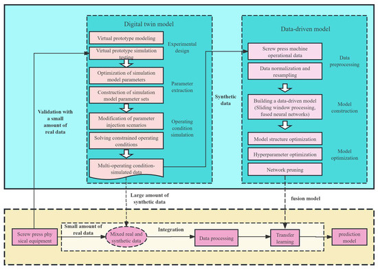
Figure 1.
The framework of the integrated fault diagnosis method for electric screw press machines.
Specifically, in this study, we first constructed a high-fidelity digital twin model using Matlab 2023b, which was proportionally consistent with the actual system. By adjusting the model parameters, we injected operational parameters under different working conditions into the twin model, generating fault data that are relatively scarce in real operating environments, addressing the issue of insufficient fault data.
To explain the results of the digital twin and support better maintenance decisions, we performed an in-depth analysis of the virtual twin model’s operational state. Through an Internet of Things (IoT)-based data acquisition and transmission system, real-time operational data from the physical system were fed back into the virtual twin model, ensuring that the virtual model dynamically updated and stayed synchronized with the actual system. The virtual data generated by the digital twin model not only provided new training data sources for the fault diagnosis model based on the latest operating conditions but also integrated historical data and real-time feedback to help the system predict potential faults and performance degradation, thereby supporting intelligent maintenance decisions.
Next, we performed feature engineering on the generated virtual data, including data normalization and resampling. After data cleaning, we applied a sliding window technique to fuse the data and input the processed data into the CNN-BLSTM-attention network for model training, ultimately resulting in a fault diagnosis pre-training model for transfer learning. Finally, the final diagnostic model was trained and optimized through transfer learning using a small amount of real data. The following sections will provide a detailed explanation of the design concepts, implementation methods, and specific applications of these two components in fault diagnosis.
3.1. Digital Twin Model
We provide a detailed description of the digital twin model used in this study. The model follows a hierarchical structure of “component–module–subsystem”, which ensures clarity and independence at each level, enabling the coordinated operation and dynamic response of the entire system.
The component layer serves as the fundamental unit for constructing the digital twin. It includes various independent physical elements such as components, actuators, and sensors. At the module layer, components are integrated based on mechanical and circuit principles to form modular components with specific functions. The subsystem layer further integrates modules to form more complex mechanical subsystems. These subsystems implement specific mechanical operational logic and numerical transmission. Finally, the integration layer integrates different subsystems to facilitate data interaction between systems, forming a comprehensive high-fidelity digital twin model. This hierarchical model comprehensively simulates and analyzes the performance and behavior of the spiral compressor. With this high-fidelity digital twin model, it is possible to understand in detail the operational states and efficiencies of the spiral compressor under various operating conditions, identify potential issues, and optimize performance adjustments.
Based on a detailed analysis of the components of the spiral compressor system, this paper simplifies the spiral compressor system into four key subsystems: mechanical system, hydraulic system, electrical system, and measurement and control system.
- Mechanical system: The mechanical subsystem is directly related to the motion of the compressor and is primarily responsible for compressing and shaping the workpiece. It includes various transmission mechanisms, guiding structures, and mechanical components to ensure the precise movement and force transmission of the compressor.
- Hydraulic system: The hydraulic subsystem maintains the balance of the compressor, ensuring stability and controllability during operation. It consists of hydraulic cylinders, valves, pumps, and other hydraulic components that control hydraulic pressure and flow to stabilize and regulate the movement of the compressor during impacting processes.
- Electrical system: The electrical subsystem involves the circuits and electronic controls of the compressor, enabling electrical signal control and impacting actions. It includes motors, sensors, controllers, and electrical circuits which ensure that mechanical components operate according to predefined logic and sequence.
- Measurement and control system: The measurement and control subsystem is responsible for parameter measurement and logic control. Its main function is to detect the status of other subsystems, provide timely feedback on monitored status information, and make corresponding decisions and controls. It includes various sensors, data acquisition devices, and control algorithms to ensure the efficient operation and real-time monitoring of the entire compressor system.
The specific structure of the digital twin model is illustrated in Figure 2, showing the relationships between these subsystems. This structured model enables the comprehensive simulation and analysis of the operational state of the spiral compressor, facilitating optimization of its performance and efficiency.
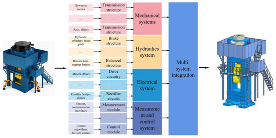
Figure 2.
Digital twin model structure.
3.2. Integrated Diagnosis Model
This section provides a detailed study of the proposed fusion model, which consists of sliding window processing, a CNN layer, a BLSTM layer, an attention layer, and a fully connected layer, as shown in Figure 3. In the following sections, we will elaborate on the specific implementation and functionalities of each component.
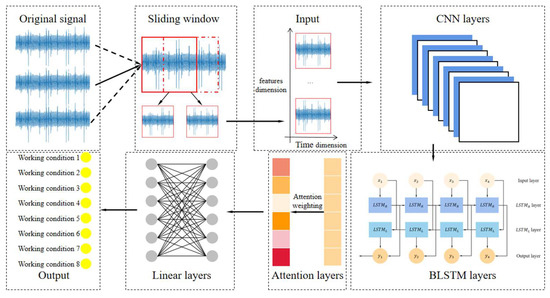
Figure 3.
Proposed integrated diagnosis model CNN-BLSTM-attention.
3.2.1. Sliding Window Processing
In the sliding window processing layer, due to the fact that the original one-dimensional samples only contain feature information and lack temporal information to assist in fault diagnosis tasks, we comprehensively considered both feature and temporal information of the target. This is achieved by processing the original data X, resulting in two-dimensional samples that integrate feature and temporal information. The processed two-dimensional samples are utilized in the proposed fusion diagnostic model, enabling the model to simultaneously learn feature and temporal information, thereby enhancing the performance of fault diagnosis. Compared to models that only consider feature information, models that incorporate both feature and temporal information can better capture the dynamic characteristics of the target system, thereby improving the accuracy and robustness of fault diagnosis. The sliding window processing procedure is illustrated in Figure 4.
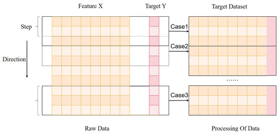
Figure 4.
Schematic diagram of sliding window processing.
3.2.2. CNN Layer
A convolutional neural network (CNN) layer consists of two main components: the convolution operation and the activation operation. The input to the convolution operation is a three-dimensional data structure , where the dimensions represent the width, height, and number of channels of the input data. Specifically, when = 1, the three-dimensional input is transformed into a two-dimensional data format, which serves as the input to the model. Specifically, the horizontal axis represents the feature vectors, and the vertical axis represents the time series, determined by the feature vectors’ input and the width of the sliding window.
To further elaborate on the convolution operation, we first define four hyperparameters: the number of convolution kernels , the size of the convolution kernels (), the stride of the convolution S, and the amount of padding . For each convolution kernel, the input datum is padded with to produce the output , and then sliced according to the size of the convolution kernel. Each slice is element-wise multiplied with the kernel and accumulated to produce the output of the convolution operation. The width and height of the output can be determined as follows:
and
In the convolution operation, each convolution kernel produces one channel of output. With convolution kernels, a new three-dimensional data structure is obtained. The convolution process is illustrated in Figure 5.
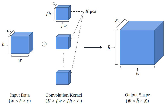
Figure 5.
Convolution operation with multiple convolution kernels.
After convolutional operations, it is necessary to apply an activation function to the output. The purpose of the activation function is to introduce non-linear expressive power, enabling the model to learn more complex feature representations and enhancing its learning capability. A common activation function is the Rectified Linear Unit (ReLU), which activates each element in the output of the convolutional operation as follows:
Here, represents each element in the output of the convolution operation.
3.2.3. BLSTM Layer
A Bidirectional Long Short-Term Memory (BLSTM) network consists of two independent LSTM networks: one for processing the forward input sequence and the other for processing the backward input sequence. Each LSTM network internally includes a forget gate, an input gate, and an output gate. The forget gate determines which information needs to be forgotten, the input gate determines which information needs to be retained, and the output gate decides which information needs to be outputted. The specific computational processes of these three gates are shown in Figure 6.
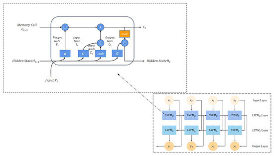
Figure 6.
Interactive layers within the repeating module of the BLSTM.
In the forget gate, the information that needs to be discarded can be identified through the following process:
Here, represents the data at time step , represents the output at the previous time step , and are the weight matrices associated with and respectively, and is the corresponding bias vector.
In the input gate, the information that needs to be input can be determined as follows:
and
Here, , and , are the weight matrices associated with and , respectively; and is the corresponding bias vector.
In the output gate, the information that needs to be output can be determined as follows:
Here, and are the weight matrices associated with , while is the corresponding bias vector.
Finally, using the state value at time step , the output and the cell state of the unit can be obtained as follows:
and
Here, denotes the element-wise multiplication.
3.2.4. Attention Layer
In traditional neural networks, the influence of different inputs on the output result is the same. However, when solving real-world problems, different inputs often have varying levels of impact on the output. To address this issue, we introduce the additive attention mechanism. Through the additive attention mechanism, we can compute the attention weights of each input element, allowing the model to selectively focus on different parts of the input. In this way, the neural network can dynamically adjust the importance of each input element based on its relevance to the current context, obtaining the attention weight for each input element, thus improving the model’s expressive power and performance. The specific computation is illustrated in Figure 7.
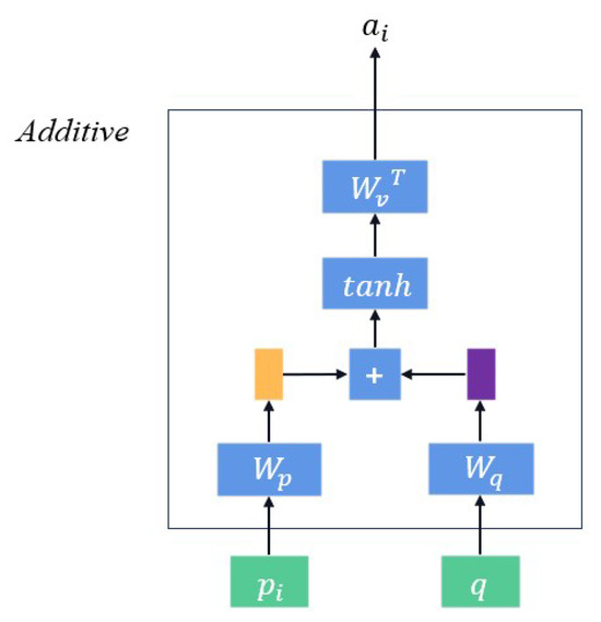
Figure 7.
Flowchart of computing additive attention.
The proposed model is related to the state at time step , using an additive model to compute the relevance function. The specific calculation process is as follows:
and
Here, the query vector q represents the state value at time step t, represents the output of the hidden layer, denotes the computed weight of , while , are the matrices associated with s.
4. Experiments and Results
4.1. Twin Dataset
4.1.1. Theoretical Construction of Twin Data
Twin data refers to all data obtained in the digital twin system through the connection and integration of different modules. These data typically include measured data, simulation data, and service data.
Taking a spiral compressor as an example, the physical data of this system should cover the external dimensions of each component, dependencies between modules, and real-time data collected by sensors. These physical data provide detailed information about the equipment’s physical characteristics and operational status. Simulation data, on the other hand, includes data generated during simulation and prediction processes such as physical models and dynamic models. Through complex calculation and simulation techniques, these data predict the equipment’s performance and response under different operating conditions, providing scientific basis for design optimization and fault prevention. Service data record the operational history of the spiral compressor, equipment maintenance information, and other relevant operational data. These data reflect the equipment’s usage status, maintenance records, and historical failure information.
By comparing and fitting measured data, simulation data, and service data, simulation data can more accurately reflect the actual operational conditions of the physical equipment.
4.1.2. Construction Process of Twin Data
The experimental data were generated using a high-fidelity digital twin model to ensure accuracy and reliability in the simulation. During the fault analysis of the electric screw press, several typical fault modes were identified, including circuit aging, hydraulic failure, and rail aging. To investigate these fault modes in depth, we selected seven representative fault conditions and their corresponding key input variables based on the multi-physics simulation model of the screw press digital twin. These input variables include motor stator resistance, rail friction, and hydraulic valve push-out force.
During the simulation process, the parameters of the relevant input variables were adjusted according to different fault modes. For example, in the cases of rail aging and normal operation, the friction coefficient was set to 0.30 and 0.05, respectively. MATLAB2023b software was then used to simulate the operational state of the screw press. The simulation yielded 40 key output variables, including flux, rotational speed (Nr), and electromagnetic torque (Te). Finally, these data were uniformly stored in .csv file format for subsequent training and evaluation of the fault diagnosis model. These output variables comprehensively reflect the operational status of the spiral compressor under different operating conditions:
Table A1 provides a detailed description of various output variables, including characteristics and parameters of various output signals. Table A2 comprehensively documents the output signal characteristics of the spiral compressor under different operating conditions, specifically covering seven fault states and one normal operating state. Each operating condition consists of 332,196 samples, resulting in a total of 8 different operating states with 8 × 332,196 = 2,657,568 original samples.
4.2. Comparative Experiments
To validate the superiority of the proposed DCBA fault diagnosis model, we conducted comparative experiments with traditional machine learning methods (e.g., SVM) and classical deep learning methods (e.g., CNN, LSTM, and ANN). We evaluated the models based on metrics such as prediction accuracy(PA), Noise Suppression (NS), and Recall Rate (RC) to determine their effectiveness.
4.2.1. Data Preprocessing
First, corresponding label attributes were assigned based on the different operating conditions in the original dataset. To ensure the representativeness and robustness of the training data, we adopted a random splitting strategy, dividing the original data into training and testing sets in a 2:8 ratio. This approach effectively avoids biases that may arise from rule-based splitting, thereby enhancing the model’s generalization ability and robustness. During the algorithm evaluation, we paid special attention to avoiding any data leakage between the training and testing sets. To achieve this, we ensured that each sample in the split data remained independent between the training and testing sets, with no shared information.
To further optimize the model’s input data, we employed a sliding window technique to construct the training-validation dataset. Based on an analysis of the original data’s temporal characteristics and multiple experimental results, we observed that fault signals exhibit distinct features within relatively short time windows. Consequently, we set the sliding window step size to 1 and the window size to 10. This parameter configuration effectively balanced the model’s ability to capture data features while enhancing its generalization ability and predictive accuracy. Specifically, a window size of 10 meant that for each movement of the sliding window by one time step, 10 consecutive data points were extracted as a sample, enabling the model to fully leverage the temporal dependencies in the data and improve its ability to capture fault characteristics.
4.2.2. Experimental Setup
To ensure the validity and comparability of the experimental results, we established the following requirements for the proposed network model and the control network models:
- For the control models included in the comparison, parameters and network layers should be as consistent as possible. For instance, for layered models, we set the number of layers to be equal and strived to maintain consistency in other model parameters, as detailed in Table 1.
 Table 1. Detailed settings of comparative experimental model parameters.
 - To improve the efficiency of the diagnostic model, we incorporated regularization and Dropout techniques into the network model to prevent overfitting.
These measures ensured that the experimental comparison was fair and meaningful, allowing for a clear evaluation of the proposed DCBA fault diagnosis model against traditional and classical deep learning methods.
Specifically, the convolutional layer used a 1D convolutional kernel with a kernel size of 3 to effectively capture local features in the input sequence. This choice of kernel size is not only closely related to the temporal characteristics of the data but also considers the granularity of feature extraction. A smaller kernel size allows for the extraction of low-level features, such as local patterns and short-term dependencies, while maintaining computational efficiency. Additionally, the smaller kernel size helps avoid introducing excessive parameters, reduces computational overhead, and retains sufficient temporal information to some extent. Experimental results show that a kernel size of 3 provided a good balance between feature-capturing ability and computational resources. To further model the long-term dependencies in the temporal data, this paper employed a Bidirectional Long Short-Term Memory (BLSTM) network, which enhanced the model’s understanding and predictive power of temporal patterns by considering both forward and backward information. To balance the model’s expressive power with computational efficiency, we chose 256 hidden units, which improves the model’s learning capacity without imposing too heavy a computational burden. To further enhance model performance, this paper introduced an attention mechanism, utilizing a simple additive attention structure to weigh and sum the output features from the LSTM layer, thereby focusing on the key information. To prevent overfitting, a Dropout layer was incorporated into the network, randomly dropping some neurons to improve the model’s generalization ability. Finally, the linear layer mapped the extracted features to the target output dimension to perform classification or regression tasks.
4.2.3. Evaluation Metrics
In this paper, we employed five metrics to evaluate the performance of each classification model: prediction accuracy (PA), Noise Suppression (NS), Precision (PC), Recall (RC), and F1 score. This section will provide a detailed explanation of these metrics.
Definition 1.
Let n denote the number of samples correctly predicted by the model, and m denote the total number of samples predicted by the model. Therefore, we define the prediction accuracy (PA) of the model as
PA reflects the prediction accuracy of the model. A higher PA value indicates a higher prediction accuracy, signifying better model performance.
Definition 2.
We introduce additive Gaussian white noise into the original dataset to test the model’s performance under noise interference [29]. Let be the accuracy obtained by the model under normal conditions, and be the accuracy obtained by the model after adding noise. Therefore, we define the model’s Noise Suppression (NS) as
NS reflects the model’s ability to maintain prediction accuracy in the presence of noise interference. The closer the NS value is to 1, the less sensitive the model is to noise, indicating stronger noise resistance and better model performance.
Definition 3.
Let TP be the number of true positive samples correctly predicted by the model, and FP be the number of false positive samples incorrectly predicted as positive by the model. Therefore, we define the model’s Precision (PC) as
Precision reflects the accuracy of the model in identifying positive instances. Specifically, a higher Precision indicates that a higher proportion of the samples predicted as positive by the model are indeed true positives.
Definition 4.
Let TP be the number of true positive samples correctly predicted by the model, and FN be the number of false negative samples incorrectly predicted as negative by the model. Therefore, we define the model’s Recall (RC) as
Recall reflects the model’s ability to identify actual positive samples. Specifically, a higher Recall indicates a stronger ability of the model to identify positive samples.
Definition 5.
The F1 score is the harmonic mean of Precision and Recall. Precision reflects the proportion of true positives among the samples predicted as positive by the model, while Recall reflects the proportion of true positives identified among all actual positive samples. Therefore, the F1 score can be calculated as follows:
The F1 score reflects the overall performance of the model in classification tasks. Only when both Precision and Recall are high will the F1 score be high. Therefore, a higher F1 score indicates better balance and superior performance of the model.
4.2.4. Results and Analysis
Due to the relatively few hyperparameters in the SVM model, we used a grid search algorithm to select the optimal hyperparameter combination for SVM. By employing a grid search, we systematically traversed a range of predefined hyperparameter values to find the combination that performed best on the validation set. Table 2 lists the optimal hyperparameter combination for the SVM model obtained through the grid search algorithm.
Table 2.
Optimal hyperparameters for SVM model.
Figure 8 shows the changes in accuracy (PA) and loss values during the training process for LSTM, ANN, CNN, CNN-BLSTM, Transformer, and the proposed model. In the graph, the abscissa (x-axis) represents the training epochs, while the ordinate (y-axis) denotes both the prediction accuracy (PA) and the loss values. As the number of iterations increases, both the training accuracy and validation accuracy gradually improve, while the training loss and validation loss gradually decrease and eventually stabilize. After surpassing a certain number of iterations, these values remain relatively constant. Specifically, the proposed model achieves a stable training and validation accuracy of 0.9646. For the LSTM, ANN, CNN, CNN-BLSTM, and Transformer models, their training accuracies are 0.9592, 0.9479, 0.8662, 0.9627, and 0.9632, respectively. From the illustrated data in the table, we can conclude that despite the complexity of the model and the large dataset, the proposed model does not exhibit severe overfitting. Additionally, in terms of convergence speed, the proposed model significantly outperforms the other five models. The proposed model converges within 10 iterations, while the other models require 30, 40, 45, 20, and 15 iterations, respectively.
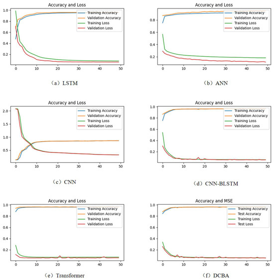
Figure 8.
PA and loss values obtained from training and validation models.
Table 3 shows the performance of different models in terms of PA. As can be seen, the proposed DCBA model outperforms traditional deep learning models and machine learning models both in results and values. This indicates a significant advantage of the DCBA model in terms of PA. The success of the DCBA model may be attributed to its integration of the strengths of CNN, LSTM, and attention modules, enabling it to handle and analyze data more effectively.
Table 3.
PA of models with noisy and noiseless data.
Specifically, when using the CNN model, the diagnostic and score decreased by 9.84% and 23.74%, respectively, compared to the DCBA model. This decline may be attributed to the fact that, while CNN excels in spatial feature extraction, it may not be as effective in analyzing sequential data as other models. Similarly, when using the LSTM model, the diagnostic and score decreased by 9.84% and 23.74%, respectively, compared to the DCBA model. Although the DCBA model demonstrated slightly better performance in these metrics, the difference is relatively small and may be influenced by random factors such as parameter initialization. Therefore, this difference should not be regarded as a significant advantage of the DCBA model over the LSTM model. However, it is noteworthy that in multiple comparative experiments, the DCBA model consistently achieved superior performance metrics compared to the LSTM model. Additionally, as shown in Table 3, the DCBA model demonstrated stronger noise resistance in factory environments with high noise interference, highlighting its potential advantage in practical applications. This improved robustness contributes to enhanced diagnostic performance in complex fault scenarios. In summary, although the LSTM model exhibits excellent performance in processing sequential data, the DCBA model demonstrates superior overall performance due to its enhanced noise resistance and improved stability. This can be explained by the fact that the DCBA model not only integrates the sequential feature extraction capability of LSTM but also leverages the spatial feature extraction advantage of CNN and the key feature capture ability of the attention module, thereby providing more comprehensive fault diagnosis performance
Furthermore, in terms of NS (noise sensitivity), the proposed DCBA model demonstrates significant advantages over traditional deep learning models. Although slightly inferior to ANN in NS, which may be due to the complexity of the DCBA network, observations show that DCBA outperforms ANN in PA. This suggests that while the DCBA model is complex in some aspects, its overall performance and specific metrics are superior. This further indicates that integrating feature information and temporal information helps enhance the model’s diagnostic effectiveness and sensitivity to noise.
Table 4 displays the comparison of various models in terms of Precision, Recall, and F1 score, demonstrating that the proposed DCBA model outperforms traditional deep learning and machine learning models in these metrics. These results indicate significant advantages of the DCBA model in Precision, Recall, and F1 score, highlighting its superiority in comprehensive performance evaluation.
Table 4.
Comparison of Precision, Recall, and F1 score across models.
Experimental results demonstrate that the proposed DCBA model achieves outstanding performance across multiple metrics, including PA, NS, Precision, Recall, and F1 score, fully validating its effectiveness and potential in the field of equipment fault diagnosis. Although the performance improvement of the DCBA model over LSTM, CNN-BiLSTM, Transformer, and SVM in certain metrics is relatively modest, the DCBA model exhibits distinct advantages in noise robustness and complex feature extraction.
Specifically, the DCBA model demonstrates minimal performance fluctuation in noisy environments, indicating its superior robustness and stability, which enhances its diagnostic reliability under complex working conditions. Furthermore, the DCBA model effectively integrates CNN’s spatial feature extraction capability, BLSTM’s temporal sequence modeling strength, and the attention mechanism’s key feature focusing ability. This comprehensive design enables improved feature extraction and fusion, significantly enhancing the model’s performance in complex pattern recognition tasks. Such characteristics further reinforce the DCBA model’s practicality and reliability for real-world industrial applications.
4.3. Fault Mode Analysis
To gain a clearer understanding of the operational mechanism of the DCBA model, we visualized the output of each layer to observe the fault patterns learned by the model. For this purpose, we selected two different fault samples from the test set, used the trained DCBA model for prediction, and visualized the outputs of each layer in the model, as shown in Figure 9 and Figure 10.
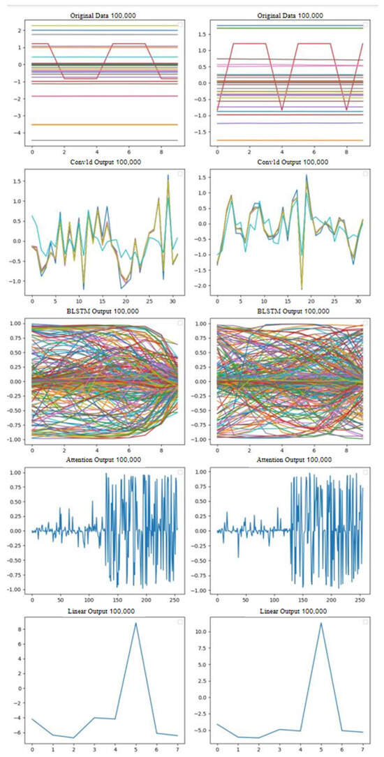
Figure 9.
A visualization of different temporal samples with the same fault.
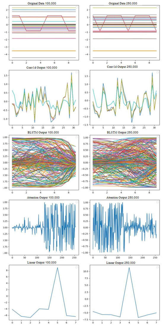
Figure 10.
A visualization of the same sample with different faults.
Specifically, in Figure 9, we selected the 100,000th and 250,000th time steps of the equipment operating under the same fault condition for prediction, and the results showed that the predictions were consistent. In contrast, in Figure 10, we selected the 100,000th time step of the equipment operating under different fault conditions for prediction, and the results showed significant differences. This indicates that the model can effectively distinguish between different fault conditions.
Based on the information reflected in the figures, we observe the following:
- After feature extraction by the CNN layer, significant features are clearly visible. This feature extraction is well demonstrated in the comparison between Figure 9 and Figure 10. The extracted features indicate a high correlation between the features captured by the CNN layer and the final fault diagnosis results. These features help the diagnostic system accurately identify and classify different types of faults, thereby enhancing diagnostic accuracy and reliability.
- The BLSTM layer further fits and models the feature data extracted by CNN. From the comparison analysis of Figure 9 and Figure 10, we can observe that in Figure 9, the curves show very similar trends and distributions, whereas in Figure 10, although the distributions of the curves are similar, there are differences in trends. This phenomenon indicates that BLSTM not only utilizes the features extracted by CNN but also leverages its advantage in capturing temporal features. These temporal features provide the diagnostic system with more comprehensive and detailed fault information, making the fault diagnosis process more reliable and efficient.
- The attention layer further processes the integrated feature data from the BLSTM layer. Based on the comparison analysis of Figure 9 and Figure 10, we can clearly observe the following: in Figure 9, there is a high similarity in data information, whereas Figure 10 shows significant differences. This demonstrates that the attention layer effectively extracts crucial information from the input features during the diagnostic process. These key pieces of information may include critical patterns, anomalous changes related to fault types, or other important features, providing decisive support and explanatory capability for the final fault diagnosis results.
- The linear layer integrates the output from the attention layer. By observing Figure 9 and Figure 10, we conclude the following: in Figure 9, data from different time points under the same fault mode are diagnosed as the same class label data, whereas in Figure 10, data from the same time points under different fault modes are diagnosed as different class label data. This observation validates the effectiveness and practicality of the proposed model in identifying faults.
5. Conclusions and Future Work
In this paper, we proposed a novel deep learning-based method that comprehensively considers data balancing, data features, and temporal information for fault diagnosis of electric screw presses. In practical applications, fault diagnosis systems must not only achieve high diagnostic accuracy but also meet the requirements for efficient computational load. To address this, we particularly focused on balancing these two aspects in the design of the DCBA model. The DCBA model combines the spatial feature extraction capabilities of convolutional neural networks (CNNs), the temporal feature modeling abilities of Bidirectional Long Short-Term Memory networks (BLSTM), and the key feature-focusing ability of the attention mechanism, resulting in excellent diagnostic accuracy. However, this high accuracy may lead to significant computational overhead. To make the DCBA model suitable for real-time applications, we reasonably simplified the network structure and adopted appropriate dimensionality reduction techniques and layer-pruning strategies to reduce the number of model parameters and computational complexity, ensuring a good balance between computational load and performance.
Experimental results show that the optimized DCBA model not only performs excellently in terms of high-accuracy fault diagnosis but also completes fault detection tasks within a reasonable time, meeting the requirements of real-time fault diagnosis systems. Especially under noisy conditions and complex operating scenarios, the DCBA model maintains high stability and efficiency, demonstrating strong potential for real-time application. Therefore, we believe that the DCBA model not only performs outstandingly in experimental settings but also has broad application prospects. Through fault diagnosis experiments on the electric screw press system, we found that this method significantly improves the diagnostic prediction accuracy and reduces sensitivity to noise. Compared with existing centralized fault diagnosis methods, the proposed approach demonstrates superior performance.
There are several aspects that warrant further research:
- This study primarily focuses on fault diagnosis of electric spiral presses, but the proposed method has broad application prospects. Therefore, further exploration of the method’s application (in fields such as chemistry, biology, and construction) to validate its generalizability and practicality remains a highly meaningful research direction. Cross-domain experimental validation will not only enhance the applicability of the method but also help improve its adaptability in real-world industrial settings.
- Introducing the attention layer into deep learning networks to improve interpretability is one of the highlights of our research. However, the reliability and stability of this method still require further improvement. Future research will focus on integrating expert knowledge, fault mechanisms, and other reliable traditional methods with deep learning techniques to enhance the robustness and accuracy of the model. By combining multiple techniques, we aim to effectively address the interpretability and reliability issues that deep learning methods face in specific fields.
- The model we proposed currently identifies fault types known during the training phase, but its ability to recognize new fault types is limited, and the model’s generalization performance significantly drops when faced with unknown faults. To address this issue, future research will focus on improving the model’s ability to identify new fault types. We plan to incorporate techniques such as few-shot learning and incremental learning to further enhance the model’s generalization ability in real-world scenarios, ensuring that it maintains efficient diagnostic capabilities even in the face of continuously evolving fault types.
- The method proposed in this study currently remains at the theoretical level. To further advance its practical application, future research will focus on the engineering deployment of the model. Specifically, we plan to integrate the model into Programmable Logic Controllers (PLC) or Industrial Edge computing devices to enhance the system’s real-time performance and stability. Furthermore, to ensure the model’s generalization capability, we will conduct on-site experiments across multiple electric screw press machines to comprehensively evaluate its performance and robustness under various operating conditions.
Author Contributions
X.H. contributed to the conceptualization, methodology, validation, formal analysis, data curation, writing of the original draft, and visualization. J.H. and J.L. were responsible for reviewing and editing the manuscript, while L.L. and Z.Q. assisted with the visualization. All authors have read and agreed to the published version of the manuscript.
Funding
This research work is supported by the Project of Department of Science and Technology of Hubei Province (Grant Number: 2023BAB055).
Data Availability Statement
Data cannot be made publicly available at the time of publication because they are owned by the project support enterprise and are prohibited from public distribution.
Conflicts of Interest
The authors declare no conflict of interest.
Appendix A
Table A1.
Screw press output variables.
Table A1.
Screw press output variables.
| Monitor Variables | Description | Unit |
|---|---|---|
| Time | Running time | s |
| Flux | Circuit flux | Wb |
| Nr | Motor outputs speed | rpm |
| Accr | Motor outputs acceleration | |
| Te | Motor output torque | N·m |
| V1 | Three-phase voltage A term of circuit | V |
| V2 | Three-phase voltage B term of circuit | V |
| V3 | Three-phase voltage C term of circuit | V |
| I1 | Three-phase current A term of circuit | I |
| T2 | Three-phase current B term of circuit | I |
| I3 | Three-phase current C term of circuit | I |
| x_R | Right hydraulic push rod pushes out displacement | mm |
| v_R | Right-hand hydraulic actuator roll-out speed | |
| a_R | Right-hand hydraulic pusher pushes out acceleration | |
| x_L | Left hydraulic push rod pushes out displacement | mm |
| v_L | Left-side hydraulic actuator roll-out speed | |
| a_L | Left hydraulic actuator pushes out acceleration | |
| Sep_R | Right hydraulic actuator is relative to flywheel | mm |
| Fn_R | Right hydraulic push rod is in contact with flywheel under normal force | N |
| Ff_R | Right hydraulic actuator is in contact with flywheel with tangential force | N |
| Sep_L | Left-side cylinder is relative to flywheel | mm |
| Fn_L | Left hydraulic actuator is in contact with flywheel under normal force | N |
| Ff_L | Left hydraulic push rod is in contact with flywheel with tangential force | N |
| Torque_flywheel | Flywheel outputs torque | N·m |
| Position_flywheel | Flywheel rotation angle | rad |
| W_flywheel | Flywheel rotation angular velocity | |
| Acc_flywheel | Flywheel rotation angular acceleration | |
| Displacement Monitoring | Position of slider relative to strike plane | mm |
| Striking Force | Striking power | KN |
| Rod_motion_v | Drive hydraulic actuator to push out theoretical speed | |
| Pressure | Hydraulic system oil pressure | MPa |
| N | Maximum theoretical speed at which drive motor operates | rpm |
| F_slider | Slider is subjected to tangential force | N |
| position_slider | Slider displacement | mm |
| v_slider | Motor outputs speed | |
| a_slider | Motor outputs acceleration | |
| GD_Ff1 | Motor output torque | N |
| GD_Ff2 | Three-phase voltage A term of circuit | N |
| GD_Ff3 | Three-phase voltage B term of circuit | N |
| GD_Ff4 | Three-phase voltage C term of circuit | N |
Table A2.
Screw press failure status.
Table A2.
Screw press failure status.
| No | Description | Type of Failure |
|---|---|---|
| 1 | All parts are normal | Normal |
| 2 | The resistance increases | Circuit aging |
| 3 | Insufficient hydraulic push-out force | Hydraulic failure |
| 4 | The coefficient of friction of a single guide rail increases | Rail aging(1) |
| 5 | The coefficient of friction of the two rails increases | Rail aging(2) |
| 6 | The coefficient of friction of the three rails increases | Rail aging(3) |
| 7 | The coefficient of friction of the four rails increases | Rail aging(4) |
| 8 | Mixed faults caused by circuit aging and rail wear | Mixed failures |
References
- Das, O.; Duygu, B.D.; Derya, B. Machine learning for fault analysis in rotating machinery: A comprehensive review. Heliyon 2023, 9, e17584. [Google Scholar] [CrossRef]
- Hosamo, H.H.; Nielsen, H.K.; Alnmr, A.N.; Svennevig, P.R.; Svidt, K. A review of the Digital Twin technology for fault detection in buildings. Front. Built Environ. 2022, 8, 1013196. [Google Scholar] [CrossRef]
- Wang, J.; Ye, L.; Gao, R.X.; Li, C.; Zhang, L. Digital Twin for rotating machinery fault diagnosis in smart manufacturing. Int. J. Prod. 2018, 57, 3920–3934. [Google Scholar] [CrossRef]
- Krizhevsky, A.; Sutskever, I.; Hinton, G.E. ImageNet classification with deep convolutional neural networks. Commun. ACM 2017, 60, 84–90. [Google Scholar] [CrossRef]
- Sun, L.; Bai, J.; Zhou, Z.; Zhao, C. Transient stability assessment of power system based on bi-directional long-shortterm memory network. Autom. Electr. Power Syst. 2020, 44, 64–72. [Google Scholar]
- Xi, X.; Xing, C.; Qin, R.; Liu, H.; Zhou, X. Power quality disturbance recognition method based on multi-layer feature fusion attention network. Smart Power 2022, 50, 37–44. [Google Scholar]
- Deebak, B.D.; Al-Turjman, F. Digital-twin assisted: Fault diagnosis using deep transfer learning for machining tool condition. Int. J. Intell. Syst. 2021, 37, 10289–10316. [Google Scholar]
- Luo, W.; Hu, T.; Ye, Y. A hybrid predictive maintenance approach for CNC machine tool driven by Digital Twin. Robot. Comput. Manuf. 2020, 65, 101974. [Google Scholar] [CrossRef]
- Liu, C.; Hsaio, W.H.; Tu, Y. Time series classification with multivariate convolutional neural network. IEEE Trans. Ind. Electron. 2019, 66, 4788–4797. [Google Scholar] [CrossRef]
- Wen, L.; Li, X.; Gao, L.; Zhang, Y. A New Convolutional neural network-based data-driven fault diagnosis method. IEEE Trans. Ind. Electron. 2018, 65, 5990–5998. [Google Scholar] [CrossRef]
- Janssens, O.; Slavkovikj, V.; Vervisch, B.; Stockman, K.; Loccufier, M.; Verstockt, S.; Van de Walle, R.; Van Hoecke, S. Convolutional neural network based fault detection for rotating machinery. J. Sound. Vib. 2016, 377, 331–345. [Google Scholar] [CrossRef]
- Guo, X.; Chen, L.; Shen, C. Hierarchical adaptive deep convolution neural network and its application to bearing fault diagnosis. Measurement 2016, 93, 490–502. [Google Scholar] [CrossRef]
- Plakias, S.; Boutalis, Y.S. Fault detection and identification of rolling element bearings with Attentive Dense CNN. Neurocomputing 2020, 405, 208–217. [Google Scholar] [CrossRef]
- Zhao, B.; Zhang, X.; Zhan, Z.; Wu, Q. Deep multi-scale adversarial network with attention: A novel domain adaptation method for intelligent fault diagnosis. J. Manuf. Syst. 2021, 59, 565–576. [Google Scholar] [CrossRef]
- Su, X.; Liu, H.; Tao, L.; Lu, C.; Suo, M. An end-to-end framework for remaining useful life prediction of rolling bearing based on feature pre-extraction mechanism and deep adaptive transformer model. Comput. Ind. Eng. 2021, 161, 107531. [Google Scholar] [CrossRef]
- Tang, H.; Tan, S.; Cheng, X. A comparative study of Chinese emotion classification techniques based on supervised learning. Chin. J. Inf. Technol. 2007, 21, 88–95. [Google Scholar]
- Wan, Y.; Gao, Q. An Ensemble Sentiment Classification System of Twitter Data for Airline Services Analysis. In Proceedings of the 2015 IEEE International Conference on Data Mining Workshop (ICDMW), Atlantic City, NJ, USA, 14–17 November 2015; pp. 1318–1325. [Google Scholar] [CrossRef]
- Ma, G.; Liu, K. Prediction of compressive strength of CFRP-confined concrete columns based on BP neural network. J. Hu′Nan Univ. (Nat. Sci.) 2021, 48, 88–97. [Google Scholar]
- Jardine, K.A.; Lin, D.; Banjevic, D. A review on machinery diagnostics and prognostics implementing condition-based maintenance. Mech. Syst. Signal Process. 2005, 20, 1483–1510. [Google Scholar] [CrossRef]
- Su, N.; Li, X.; Zhang, Q. Fault Diagnosis of Rotating Machinery Based on Wavelet Domain Denoising and Metric Distance. IEEE Access 2019, 7, 73262–73270. [Google Scholar] [CrossRef]
- Zhao, R.; Yan, R.; Chen, Z. Deep learning and its applications to machine health monitoring. Mech. Syst. Signal Process. 2019, 115, 213–237. [Google Scholar] [CrossRef]
- Du, T.; Zhang, H.; Wang, L. Analogue circuit fault diagnosis based on convolution neural network. Electron. Lett. 2019, 55, 1277–1279. [Google Scholar]
- Lee, J.; Pack, J.; Lee, I. Fault Diagnosis of Induction Motor Using Convolutional Neural Network. Appl. Sci. 2019, 9, 2950. [Google Scholar] [CrossRef]
- Sahu, A.R.; Palei, S.K.; Mishra, A. Data-driven fault diagnosis approaches for industrial equipment: A review. Expert. Syst. 2023, 41, e13360. [Google Scholar]
- Cai, J.; Xiao, Y.; Fu, L. Fault Diagnosis of Rolling Bearing Based on Fractional Fourier Instantaneous Spectrum. Exp. Tech. 2021, prepublish. [Google Scholar]
- Liu, H.; Zhou, J.; Zheng, Y.; Jiang, W.; Zhang, Y. Fault diagnosis of rolling bearings with recurrent neural network-based autoencoders. ISA Trans. 2018, 77, 167–178. [Google Scholar]
- Tang, X.; Chi, G.; Cui, L.; Ip, A.W.; Yung, K.L.; Xie, X. Exploring Research on the Construction and Application of Knowledge Graphs for Aircraft Fault Diagnosis. Sensors 2023, 23, 5295. [Google Scholar] [CrossRef]
- Wang, Z.; Liang, B.; Guo, J.; Wang, L.; Tan, Y.; Li, X. Fault diagnosis based on residual–knowledge–data jointly driven method for chillers. Eng. Appl. Artif. Intell. 2023, 125, 106768. [Google Scholar]
- Hughes, B. On the error probability of signals in additive white Gaussian noise. IEEE Trans. Inf. Theory 1991, 37, 151–155. [Google Scholar]
Disclaimer/Publisher’s Note: The statements, opinions and data contained in all publications are solely those of the individual author(s) and contributor(s) and not of MDPI and/or the editor(s). MDPI and/or the editor(s) disclaim responsibility for any injury to people or property resulting from any ideas, methods, instructions or products referred to in the content. |
© 2025 by the authors. Licensee MDPI, Basel, Switzerland. This article is an open access article distributed under the terms and conditions of the Creative Commons Attribution (CC BY) license (https://creativecommons.org/licenses/by/4.0/).