Abstract
Medical imaging is crucial for disease diagnosis, but noise in CT and MRI scans can obscure critical details, making accurate diagnosis challenging. Traditional denoising methods and deep learning techniques often produce overly smooth images that lack vital diagnostic information. GAN-based approaches also struggle to balance noise removal and content preservation. Existing research has not explored tumor detection after image denoising; instead, it has concentrated on content and noise learning. To address these challenges, this study proposes the Adversarial Content–Noise Complementary Learning (ACNCL) model, which enhances image denoising and tumor detection. Unlike conventional methods focusing solely on content or noise learning, ACNCL simultaneously learns both through dual predictors, ensuring the complementary reconstruction of high-quality images. The model integrates multiple denoising techniques (DnCNN, U-Net, DenseNet, CA-AGF, and DWT) within a GAN framework, using PatchGAN as a local discriminator to preserve fine image textures. The ACNCL separates anatomical details and noise into distinct pathways, ensuring stable noise reduction while maintaining structural integrity. Evaluated on CT and MRI datasets, ACNCL demonstrated exceptional performance compared to traditional models both qualitatively and quantitatively. It exhibited strong generalization across datasets, improving medical image clarity and enabling earlier tumor detection. These findings highlight ACNCL’s potential to enhance diagnostic accuracy and support improved clinical decision-making.
1. Introduction
Medical imaging is crucial for accurate diagnosis, utilizing CT, MRI, PET, X-ray, and ultrasound to reveal internal structures [1,2]. However, the noise inherent in these imaging techniques, such as Gaussian noise in CT and MRI, compromises image quality and challenges accurate diagnosis, particularly in detecting small lesions and tumors [3]. Traditional noise reduction methods like non-local means, wavelet transforms, and spatial filters often over-smooth images, obscuring critical details needed for tumor delineation and compromising diagnostic accuracy [4,5,6]. Recent advancements in deep learning have shown promise in medical image denoising [7]. Techniques like fractal networks (FNs) [8], variational autoencoders (VAEs) [9], and Generative Adversarial Networks (GANs) [10] have improved the visual quality of CT and MRI scans. Methods such as U-Net [11] architectures and convolutional neural networks (CNNs) [12] have effectively reduced noise and recovered degraded images. In another study [13], a denoising convolutional neural network (DnCNN) was utilized to recover MRI images degraded by Rician noise. In their work [14], they developed a sparse convolutional neural network (SCNN) along with a deep learning-based reconstruction model (DLRM) to denoise brain MR images and detect lesions. A convolutional autoencoder–decoder with residual learning (RED-CNN) [15] was successfully employed to estimate a normal-dose CT image from its low-dose counterpart. DenseNet [16] and block-matching 3D (BM3D) [17] have been used for Content–Noise Complementary Learning. While DenseNet faces high memory usage, limiting real-time noise removal, BM3D excels with Gaussian noise but struggles with structured noise and large images. A conditional GAN with a VGG (Visual Geometry Group) (CGAN-VGG) showed perceptual loss in the ability to preserve perceptual quality and fine details; that said, instability in training when balancing the adversarial and perceptual losses is challenging and often leads to overfitting [18]. The Wasserstein GAN was used in [19,20] for low-dose denoising, and the performance indicated improved training instability by reducing sudden discriminator dominance.
Despite their success, these approaches face challenges in preserving fine structural details and preventing over-smoothing [21], which are essential for detecting small tumors and maintaining diagnostic accuracy. They are faced with difficulty in detecting low-contrast noise [22], soft tissue differentiation, and low signal-to-noise ratio [23,24]. In network architecture, GAN-based denoising methods are categorized into noise learning and content learning [25]. Noise learning effectively preserves image contrast and detail [26], while content learning provides stable noise suppression [27]. Combining these strategies has led to innovative models like Content–Noise Complementary Learning (CNCL), which enhances image quality by separating content from noise [28]. However, issues like mode collapse and over-smoothing remain prevalent in GANs, highlighting the need for balanced generator–discriminator dynamics to maintain image fidelity. Existing research has not explored tumor detection after image denoising; instead, it has concentrated on content and noise learning. To address these challenges, this study proposes the Adversarial Content–Noise Complementary Learning (ACNCL) model. Recent studies have explored dual-task frameworks that integrate denoising and diagnostic tasks for enhanced clinical interpretation. For example, Reference [29] proposed a multi-task deep learning approach for simultaneous denoising and classification, achieving improved robustness to noisy data. Similarly, Reference [30] demonstrated that content-aware GANs could significantly enhance lesion visibility in low-dose CT scans. These works validate the notion that denoising should not be an isolated pre-processing step but integrated with diagnostic purposes. The proposed ACNCL model builds on this principle, uniquely leveraging adversarial training to jointly optimize for image clarity and tumor detectability. The ACNCL model integrates image denoising with tumor detection, utilizing predictors like DnCNN, U-Net, DenseNet, DWT, and CA-AGF within a GAN architecture. By using PatchGAN, the model enhances local feature detection, which is crucial for identifying subtle tumor characteristics. This approach allows simultaneous learning of content and noise, improving both denoising and tumor detection accuracy in low-quality medical images. Experimental results on CT and MRI datasets demonstrate the improved performance of the ACNCL model over traditional methods, showcasing enhanced image quality and more accurate tumor detection. The model further connects to an online database for automated second-level validation of tumorous regions, a feature not incorporated in conventional methods.
By integrating deep learning predictors with GAN-based architecture, the ACNCL model effectively balances noise reduction and content preservation, providing a robust solution for medical image denoising and tumor detection. This paper makes the following contributions to the body of knowledge:
- The ACNCL model uniquely connects image denoising with tumor detection, evaluating tumor detection performance before and after denoising. This integration addresses the gap in previous research [16], which focused solely on content and noise learning without considering the impact on tumor detection.
- The incorporation of PatchGAN as a local discriminator ensures fine-grained texture restoration and the structural integrity of medical images. The ACNCL model further enhances denoising efficiency using dual discriminators, one for real pairs and another for fake pairs, striking a balance between noise suppression and content preservation.
- Unlike traditional models that discard noise priors during testing, the ACNCL predictor model uses two predictors, content and noise, in a complementary manner. This approach allows for more effective noise removal while preserving critical anatomical details, enhancing the diagnostic quality of medical images.
2. Materials and Methods
This study adopts an experimental research design, employing both quantitative and comparative analysis to evaluate the efficacy of the proposed ACNCL model. The research design is structured into three key phases: (i) model development and implementation using GAN-based dual-path architecture (ACNCL) and its predictors, (ii) empirical evaluation using multiple publicly available CT and MRI datasets that show results before denoising (BDn) and after denoising (ADn) and results before and after ACNCL, and (iii) benchmarking against baseline models and reference denoising methods. Each model variation (ACNCL-DnCNN, ACNCL-U-Net, ACNCL-DenseNet, ACNCL-CA-AGF, ACNCL-DWT) was trained and tested using standardized metrics (PSNR, SSIM, RMSE) and validated across cross-contextual datasets to ensure generalizability. Ablation studies further explored individual predictor contributions to the overall model’s performance.
The ACNCL model incorporates a variety of CNN architectures and signal processing techniques for medical image denoising and tumor detection. The model utilized the following techniques:
- a.
- U-Net
U-Net is a deep learning architecture that preserves spatial details using skip connections, reducing information loss during encoding and decoding. The skip connections combine encoder and decoder features as follows:
where “Combine” represents concatenation () or element-wise addition (+), ensuring the retention of spatial and contextual information for accurate segmentation.
- b.
- DnCNN
DnCNN is a neural network that learns residual noise in an image, making denoising more efficient by predicting noise rather than the clean image. The clean image is then reconstructed as
where is the noisy image, is the predicted noise, and is the denoised output.
- c.
- DenseNet
DenseNet enhances feature reuse and gradient flow by connecting each layer to all previous layers. The output of each layer is computed as
where is the feature map at the layer is the initial input, and represents convolution and activation operations.
- d.
- Context-Aware Anisotropic Gaussian Filtering (CA-AGF)
CA-AGF is a spatial filtering technique that adapts to local image structures, smoothing noise while preserving edges and textures. The filtered image is computed as
where is the input image, is the Gaussian kernel, and is a context-aware weight that adjusts smoothing based on local gradients.
- e.
- Discrete Wavelet Transform (DWT)
DWT decomposes an image into low- and high-frequency components, enabling noise removal while preserving important structural details. The decomposition and reconstruction are expressed as
where represents the low-frequency approximation, preserving the main structure, while captures high-frequency details and noise. The inverse DWT (IDWT) combines these components to reconstruct the original image with selective noise removal.
- f.
- Generative Adversarial Networks (GAN)
GANs use a generator to create denoised images and a discriminator to distinguish real from fake, enhancing image quality for medical tasks like tumor detection. It is formulated as follows:
Generator Loss (content learning):
where is the generated clean image, and is the target clean image.
Discriminator Loss (Real vs. Fake):
where classifies real images, and classifies generated images.
Content and Noise Learning:
where represents important structures (e.g., tumors), and represents noise.
Total Loss Function:
where and balance content and noise learning.
Diversity Loss (Avoiding Mode Collapse):
where is a different input to encourage diverse outputs.
Therefore:
2.1. Mathematical Formulations for Detecting Gaussian Noise in CT and MRI Images
Preliminary: In conventional image denoising and tumor detection models, the training processes for these two tasks are typically separate. We aim to integrate the denoising and detection tasks into a unified model. To detect Gaussian noise in CT and MRI images, we first need a mathematical noise model, followed by a model for estimating the parameters of Gaussian noise, typically the mean and variance (). Here is a structured approach:
- i.
- Gaussian Noise Model
In imaging, Gaussian noise can be mathematically represented as:
where represents a normal Gaussian distribution with the mean and variance .
- : The mean of the distribution, indicating the central value around which noise values are distributed.
- : The variance of the distribution, indicating the spread of noise values around the mean. A higher variance corresponds to greater deviations from the mean.
Gaussian noise is a bell-shaped curve where most noise values are concentrated near the mean, , with fewer extreme deviations. For a noisy image , the observed image is modeled as the sum of the true image and Gaussian noise :
Here, is the noisy image (CT or MRI), is the underlying clean image that we aim to recover, and is the Gaussian noise that affects the image.
- ii.
- Estimating Gaussian Noise Parameters (Mean and Variance)
Gaussian noise estimation involves assessing the noise in regions assumed to be homogeneous (i.e., areas with little to no variation due to tissue uniformity). Here are the steps for estimating and :
Mean () Estimation
Since Gaussian noise is often assumed to have a zero mean in medical images, an initial assumption is
However, in cases where there might be a slight bias, we can estimate the mean. of the noise using a region in the image where the intensity is relatively constant:
where is the number of pixels in the selected homogeneous region, and is the pixel values.
Variance () Estimation
To estimate , we calculate the variance of pixel values in the homogeneous region. Given a sample of pixel values in this region, the variance can be estimated as:
An alternative approach, particularly in larger images, is to use a sliding window over the image to calculate local variance. The average of these local variances provides an estimate of .
- iii.
- Overall Noise Detection Formula
Bringing it all together, the formula for Gaussian noise detection in a given CT or MRI image region is:
where
- represents the pixel intensities in a homogeneous image region;
- is the number of pixels in this region;
- and represent the mean and variance of Gaussian noise in that region, providing essential parameters for further denoising.
2.2. Adversarial Content–Noise Complementary Learning (ACNCL)
Under ACNCL (Adversarial Content–Noise Complementary Learning), we tackle the problem of denoising medical images, particularly CT and MRI scans, by leveraging an innovative approach that incorporates GANs as key components in learning both content and noise features simultaneously. This model combines both noise and content prediction, ensuring improved denoising while preserving structural details critical for medical diagnosis. Consider an image denoted as which has been compromised by noise due to low-dose imaging or under-sampling techniques. The corresponding high-quality image, free from such degradation, is represented as In the context of deep learning-based denoising for medical images, can be conceptualized as the sum of its undistorted sub-content and the additive noise component
(a) Noise Identification and Context Partitioning: The denoising process begins with the Noise Identifier (ACNCL-Part 1), which detects the noise type present in the input image . Noise in medical images often arises due to low-dose imaging or under-sampling techniques, which can obscure crucial features.
A Context Partitioning step follows, where noisy images are separated based on the extent and type of noise, allowing for tailored reconstruction. This partitioning facilitates efficient denoising by focusing on relevant noise patterns in each image segment.
(b) Content and Noise Prediction: In the denoising model, content prediction aims to recover the underlying noise-free image . Given a degraded input image , we obtain a predicted clean image by applying a content predictor :
In contrast, Residual Mapping (noise prediction) estimates the noise component. The clean content can then be derived by subtracting this predicted noise from :
Here, represents the noise predictor, and is the estimated noise component. This approach balances consistency and detail preservation by combining the strengths of both content and noise prediction.
(c) Adversarial Content–Noise Complementary Learning (ACNCL) Integration: The ACNCL model harmonizes the outputs of (content predictor) and (noise predictor), framing denoising as an end-to-end learning task. The final predicted content image is generated using a fusion function that combines the outputs from content and noise prediction:
Here, and represent the outputs from the content predictor and the noise-derived content, respectively. The fusion function integrates both predictions to yield the final denoised result. In the ACNCL denoising model for image denoising and tumor detection in low-quality images, we utilized two training pairs derived from each image as shown in Figure 1:
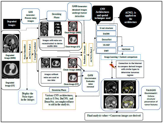
Figure 1.
Adversarial Content–Noise Complementary Learning (ACNCL) denoising architecture for image denoising and tumor detection in low-quality medical images.
- The pair is used to train the content predictor , focusing on reconstructing clean content.
- The pair is used to train the noise predictor , which learns to isolate noise patterns.
- This training approach enables the network to learn complementary aspects of noise and content synergistically.
The process in Figure 1 shows a GAN-based approach integrated with Content and Noise Complementary Learning (ACNCL) for MRI and CT image denoising and tumor detection. The process begins with degraded medical images, which may contain different types of noise. The Noise Identifier (ACNCL-Part 1) first analyzes these images to classify the content and noise types present. Noisy images are then passed through a GAN Generator, which removes noise while reconstructing useful image data. Meanwhile, raw images without noise are also fed into the system for comparison and validation. The GAN Discriminator evaluates the effectiveness of noise removal by distinguishing between the denoised and real clean images. Various CNN architectures like U-Net, DnCNN, DenseNet, DWT, and CA-AGF are then applied to enhance the denoised images, ensuring that important structures are preserved while refining the image quality. After enhancement, the ACNCL-Part 2 predictor is used to detect potential tumor regions in the clean images.
The tumor detection results undergo further refinement using PatchGAN, which enforces structural preservation of the tumor features. The processed images are then compared with a medical database to verify and confirm the presence of tumors based on similar cases. This image learning and content comparison phase helps improve detection accuracy. Finally, the model outputs highlighted tumor regions along with an analysis of their severity, providing valuable diagnostic insights. The final results present tumor-marked MRI/CT images, ready for medical evaluation and treatment planning.
2.3. Flowchart Representation of the Proposed ACNCL
The flowchart in Figure 2 illustrates a structured approach to denoising and tumor detection in MRI and CT images using a Generative Adversarial Network (GAN)-based model integrated with Content and Noise Complementary Learning (CNCL). It starts with loading noisy MRI/CT images, followed by identifying noise types using ACNCL-Part 1, which classifies noise for appropriate processing. The GAN Generator then removes noise while reconstructing useful image data, and the GAN Discriminator evaluates the effectiveness of this denoising process. The denoised images are further enhanced using CNN-based methods, including U-Net, DnCNN, DenseNet, DWT, and CA-AGF, to improve structural clarity. The ACNCL-Part 2 predictor detects potential tumor regions in the processed images, after which PatchGAN ensures the structural preservation of tumor features. The refined images are compared with external medical databases to confirm tumor regions, and the final output presents tumor-marked images with diagnostic insights for medical evaluation.
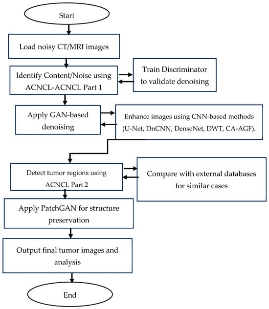
Figure 2.
Flowchart representation of the proposed ACNCL model for image denoising and tumor detection in low-quality medical images.
3. Implementation Based on Generative Adversarial Network (GAN)
The ACNCL denoising and tumor detection model leverages Generative Adversarial Networks (GANs) to separate content and noise in medical images, enhancing denoising and tumor detection. GANs are increasingly preferred over traditional CT and MRI scan methods due to their ability to model complex noise distributions. Unlike conventional techniques, GANs learn to differentiate noise from essential structures, preserving critical details like tumor boundaries. This results in sharper images optimized for tumor detection.
Compared to Convolutional Neural Networks (CNNs), generative adversarial networks (GANs) offer a key advantage in generating high-quality images through adversarial training. While CNNs excel at feature extraction and classification, they typically require separate pre-processing for denoising before tumor detection. In contrast, GANs integrate noise removal and feature enhancement into a single process, improving generalization across diverse datasets. Despite their advantages, GANs face challenges such as mode collapse, where the generator produces limited variations and misses diverse tumor features. Additionally, over-smoothing may blur fine details, and training instability makes balancing the generator and discriminator difficult. To address these issues, adversarial training ensures that the discriminator learns to distinguish clean from noisy images, improving the generator’s ability to retain tumor details while denoising effectively. To mitigate mode collapse, loss functions are adapted to penalize repetitive outputs, encouraging the generator to explore diverse image regions. This is essential in tumor detection, where variations in tumor shapes and structures exist. Training stability is enhanced through ACNCL’s dual-task learning approach: one part of the network focuses on denoising, while another addresses tumor detection. This division provides clear denoising while preserving essential structures. By training the generator alongside a discriminator that distinguishes clean and noisy images, ACNCL generates realistic, high-quality outputs without over-tuning to specific noise patterns, ensuring robust tumor detection and improved medical image clarity.
- 1.
- The GAN architecture: It is structured with two primary components: a Generator and a Discriminator. The Generator uses multiple predictors, such as DnCNN, U-Net, and DenseNet, to process the degraded image, separating it into predicted content and predicted noise. The Generator also incorporates wavelet transformations (DWT) and a Context-Aware Anisotropic Gaussian Filter (CA-AGF) to enhance the accuracy of the predictions. The Discriminator Patch GAN architecture is employed, which is responsible for distinguishing between real and generated image pairs (i.e., real content vs. predicted content). The Discriminator also evaluates the tumor detection accuracy by incorporating specialized loss functions that penalize incorrect predictions of tumor regions.Figure 3 shows a GAN-based implementation of the proposed ACNCL model. The diagram is organized into several interconnected components:
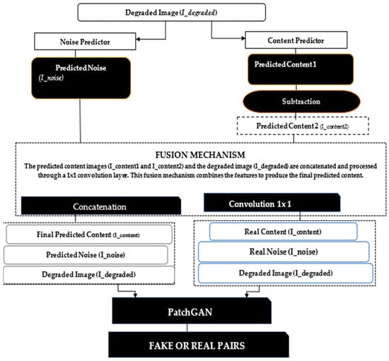 Figure 3. The architecture of a GAN-based implementation of the Adversarial Content–Noise Complementary Learning (ACNCL) model for image denoising and tumor detection.Input Degraded Image (I_degraded): The degraded medical image, potentially containing a tumor, is passed through the Noise Predictor and Content Predictor sub-networks within the Generator.Noise Predictor (GAN-based): The noise predictor leverages models like U-net and DenseNet to estimate the noise components in the degraded image. It incorporates Discrete Wavelet Transform (DWT) and Context-Aware Anisotropic Gaussian Filter (CA-AGF) extraction to capture and enhance the noisy regions. The output is the Predicted Noise (I_noise).Content Predictor (GAN-based): Simultaneously, the degraded image is processed through the content prediction pathway. Models such as U-net and DenseNet are used to predict the underlying clean content, focusing on preserving key diagnostic features like potential tumors. The output here is the Predicted Content (I_content1).Subtraction and Fusion Mechanism: The predicted noise (I_noise) is subtracted from the degraded image (I_degraded) to yield an intermediate prediction, which undergoes further refinement. A Fusion Mechanism then concatenates and processes the predicted content and noise through additional layers (e.g., convolutional layers and AGF extraction), producing the final predicted content (I_content2).Tumor Detection: The tumor detection mechanism is embedded within the Generator, where the final predicted content is analyzed using specific features to identify potential tumors. DenseNet plays a key role in enhancing detection accuracy by learning complex patterns associated with tumor regions.Discriminator (PatchGAN): The Discriminator receives real and fake pairs. Real Pairs: The real content (I_content) and real noise (I_noise). Fake Pair: The final predicted content (I_content2) and the original corrupted image (I_degraded). The Discriminator evaluates the authenticity of the generated images and the accuracy of tumor detection, feeding back the results to refine the Generator’s predictions. The final output from the Generator is a denoised medical image with tumor regions. The Discriminator ensures that the generated image is not only noise-free but also preserves critical diagnostic features, such as tumors, for reliable medical analysis. PatchGAN, a well-known Discriminator, targets structural inconsistencies at the patch level, addressing common issues like texture or style degradation. To tackle this problem, we incorporated PatchGAN as the Discriminator in our proposed GAN model. PatchGAN processes either a set of real images. or a fake image pair generated as an image set as inputs. The Generator’s objective is to produce synthetic data that can deceive the Discriminator, while PatchGAN focuses on differentiating between synthetic and real data.PatchGAN is significant in medical imaging tasks because it focuses on local image patches rather than the entire image, allowing it to effectively capture fine-grained details that are crucial in medical diagnostics, such as tumor boundaries or subtle variations in tissue structures. By operating on smaller regions of the image, PatchGAN learns to differentiate between small-scale features, which is especially important in applications like tumor detection, organ segmentation, or lesion identification, where local abnormalities need to be detected with high accuracy.
 - 2.
- Loss Function: To define the loss function, we followed the approach suggested by [31], using a combination of PatchGAN loss and L1 loss. This composite loss function, denoted as , is formulated as follows:where represents the GAN loss (based on PatchGAN), is the L1 loss, and is a weighting coefficient for the L1 component.The GAN loss is expressed aswhere denotes expectation, is the Generator, is the Discriminator, represents the degraded image and yields the estimated noise and content components and . In this model, the Discriminator seeks to maximize this objective, while the Generator attempts to minimize it.The L1 loss, , is separated into two distinct parts:Here, LL1-content quantifies the mean absolute error between the generated content and the actual content , while measures the mean absolute error between the predicted noise and the true noise . The parameter serves as a scaling factor for .
Experimental Setup
In this study, multiple deep learning architectures and signal processing techniques were integrated into a Generative Adversarial Network (GAN) framework for medical image denoising and tumor detection. The ACNCL model employs dual predictors: one for content preservation and another for noise estimation, allowing a complementary learning strategy. CNN-based architectures such as U-Net, DenseNet, and DnCNN are optimized using modified parameters such as replacing deconvolution with sub-pixel convolutions and applying Atrous Spatial Pyramid Pooling (ASPP) to enhance multi-scale feature extraction. Pre-processing involved normalization and resizing of image slices from CT and MRI datasets, which were then augmented using rotation and flipping to improve model robustness.
(i) Predictors: To demonstrate the effectiveness of the proposed ACNCL model, we explored various predictors within our GAN-based model. Table 1 gives a summary of the predictors’ contribution, including DnCNN, CA-AGF, DWT, U-Net, and DenseNet.

Table 1.
Summary of contributions of predictors (DnCNN, DenseNet, U-Net, CA-AGF, and DWT) to the overall performance.
Table 1.
Summary of contributions of predictors (DnCNN, DenseNet, U-Net, CA-AGF, and DWT) to the overall performance.
| Predictor | Original Form | Modification | Overall Performance |
| U-Net (Figure 4a) [11] | -Unified one U-Net -No Paddling applied -No batch normalization | -Compared to U-Net in [11] our architecture is split into two parallel pathways (one for content and the other for noise). -Padding applied to maintain consistent feature map size before and after convolution. -Batch normalization is introduced to stabilize the training process by normalizing layer activations. | -Enhances ability to separate and utilize noise-related and content features for effective capturing and processing. -Padding allows accurate alignment and combination of high-level and low-level features across the network. -Faster convergence and improved denoising performance. |
| DnCNN (Figure 4b) [13] | -DnCNN originally used residual learning, where the network learned to predict the noise rather than the denoised image itself -DnCNN used the standard ReLU (Rectified Linear Unit) activation function after convolution layers | -In contrast with DnCNN in [13] this work discarded the residual learning since noise can dominate residuals. -Leakey ReLU is used in place of standard ReLU. | -The network is trained directly to output the denoised image rather than the noise residual. Residual was removed to prevent over-smoothing. -Leaky ReLU allows a small, non-zero gradient for negative values, thereby preventing dead neurons and allowing better information flow through the network. |
| DenseNet (Figure 4c) [16] | -Used deconvolution layers -Bottleneck layers -Traditional reconstruction layers | -Sub-pixel convolution replaced deconvolution bottleneck. -Atrous Spatial Pyramid Pooling (ASPP) substituted bottleneck layers. -Cascaded Refinement Network (CRN). | -Reconstruction layers used to produce smoother and more accurate up-sampled images. -Captures multi-scale contextual information without reducing spatial resolution, allowing for better feature preservation and enhanced localization of tumors in noisy medical images. -Higher quality and more accurate denoised outputs. |
| CA-AGF (Figure 4d) [5] | -Traditional AGF has no dynamism in the filtering process | -The Context-Aware AGF dynamically adjusts the filtering process based on local image structures. | -Enhances feature preservation and denoising adaptability in complex regions like medical images. |
| DWT (Figure 4e) [6] | -Traditional DWT produces less natural-looking and less detailed denoised images. | -Enhanced with multi-resolution fusion and anisotropic diffusion to preserve fine details and broader structures. | -Produces more natural-looking and detailed denoised images compared to the original DWT. |
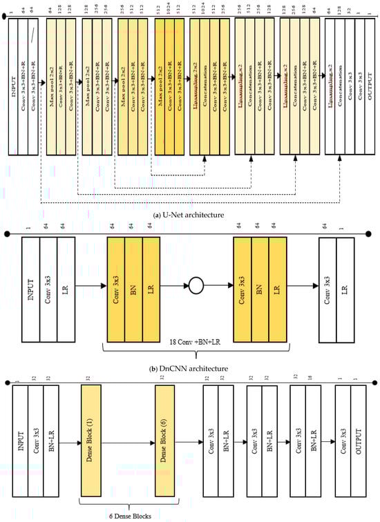
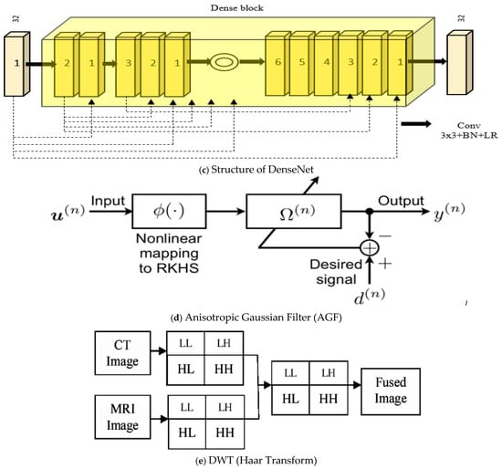
Figure 4.
(a–e) The CNN architectures, CA-AGF, and DWT utilized as predictors in our GAN-based implementation are illustrated.
(ii) Dataset Description
- (a)
- CT Dataset: The proposed denoising model was validated on a publicly available CT dataset collected from The Cancer Genome Atlas Lung Adenocarcinoma (TCGA-LUAD) specifically curated for evaluating medical image denoising techniques [32]. This dataset can be accessed at this link: https://www.cancerimagingarchive.net/collection/tcga-luad/, accessed on 5 May 2020. The dataset comprised 10 CT scans from anonymous patients, each containing 2D slices of abdominal regions and corresponding simulated 25% dose CT 2D slices. The full-dose data were acquired at 120 k and 220 effective mAs, while the 25% dose data were generated by adding Poisson noise into the projection data. The dataset included 2428 2D slice pairs (512 × 512 pixels). We selected 1830 slice pairs from 7 patient scans for training and 598 CT slice pairs from 3 patients for testing. Another set of brain datasets for CT images was used to compare the performance of the results obtained. The dataset had dimensions of 512 × 512 pixels and is a collection of human brains with neurological conditions, including cancer, tumors, and aneurysms. The dataset can be accessed at https://www.kaggle.com/datasets/trainingdatapro/computed-tomography-ct-of-the-brain/data, accessed on 13 December 2024.
- (b)
- MRI: The dataset used in this experiment is a curated combination of three sources: the Figshare dataset, the SARTAJ dataset, and the Br35H dataset. The Figshare dataset provided a significant portion of the images, particularly for the glioma class, which was critical due to issues identified in the SARTAJ dataset. The SARTAJ dataset initially included images for various tumor classes, but it was noted that the glioma class images were not accurately categorized. To ensure the integrity of the experiment, these images were replaced with more reliable ones from the Figshare dataset. Finally, the Br35H dataset supplied the no-tumor class images, which were necessary for the negative class in the classification tasks. The dataset can be accessed at this link: https://www.kaggle.com/datasets/masoudnickparvar/brain-tumor-mri-dataset, accessed on 4 January 2021. It contained abdomen 2D slices of 10 patients in a clinical trial containing 1311 2D slice pairs in total (544 × 394 pixels). Four classes were categorized into Figshare, SARTAJ, Br35H, and pituitary tumors. We selected 991 slice pairs from 8 patients for training and 320 slice pairs from 2 patients for testing. Additionally, we used a dataset from the Stanford Brain MRI dataset comprising 156 whole-brain MRI studies [33].
(iii) Data Preparation and transformation
In this experiment, we focused on MRI and CT images as our datasets. To thoroughly assess the efficacy of the proposed denoising and tumor detection approach, we evaluated ACNCL-U-Net, ACNCL-DnCNN, ACNCL-DenseNet, ACNCL-CA-AGF, and ACNCL-DWT using four distinct medical imaging datasets. These datasets span two imaging modalities commonly used in clinical diagnostics: CT and MRI. The noisy CT was collected under low-dose conditions, while the noisy MRI images resulted from k-space under-sampling. Figure 5 illustrates examples of two image slices, highlighting the significant differences in noise patterns across the various imaging modalities. The degraded medical images, the corresponding clean images, and the noisy images in two medical imaging modalities are shown.
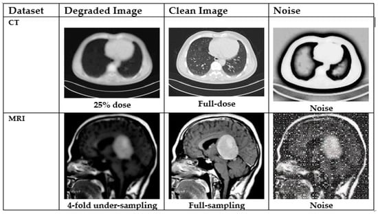
Figure 5.
Degraded medical images (the leftmost column), the corresponding clean images (the middle column), and the noise (the rightmost column) in two medical imaging modalities. From the top to bottom row: CT and MRI.
(iv) Description of training: During the training phase of our GAN-based implementation for the ACNCL model, the architecture was implemented on PyTorch version 24, and training was conducted on an NVIDIA GeForce RTX 2080Ti GPU; Nvidia Corporation; California-USA, which provided the necessary computational power to handle the deep learning tasks efficiently. The Adam optimizer [34] was employed for training all networks in the experiment. The momentum parameters for Adam were set. The Momentum 1 (β1) of parameter 0.5 controls the exponential decay rate for the first-moment estimate (the running average of gradients). A β1 value of 0.5 introduces some level of smoothing by making the algorithm focus on recent gradients but not heavily weighing them, which helps avoid sharp oscillations. The Momentum 2 (β2) of 0.999 controls the exponential decay rate for the second moment estimate (the running average of squared gradients). With a value close to 1 (0.999), Adam efficiently captures the variance of gradients over time, leading to a more stable convergence by reducing oscillations. These settings help in controlling the moving average of gradients, where β1 controls the first moment (mean) and β2 controls the second moment (variance). The learning rate was set to 0.0002, which is a typical value for training Generative Adversarial Networks (GANs) and other deep learning models. A small batch size of 2 was chosen for training. The weights λ1 and λ2 in the equations were set to 1 and 100, respectively. The weights λ2 were specifically derived from the PatchGAN, which suggests an appropriate setting for discriminative networks focusing on texture and detail preservation. Weight λ1 was determined through a range of experiments to optimize denoising performance while maintaining the quality of tumor detection. Before training, the initial weights for convolutional layers and batch normalization layers were initialized with random numbers from a normal distribution and in this case, for convolutions, weights were sampled from N (0, 0.021) N (0, 0.021) N (0, 0.021), where the mean is 0 and the standard deviation is 0.021. For batch normalization, weights were initialized with N (1.0, 0.021) N (1.0, 0.021) N (1.0, 0.021), and biases were set to 0. The training of all networks was carried out over 300 epochs. The 300 epochs provided a balance between overfitting and underfitting; in underfitting, fewer epochs may result in an under-trained model, while in overfitting, training for too many epochs risks the model learning noise or irrelevant features from the training set, resulting in poorer performance on test data. By employing strategies like early stopping or weight regularization, training over 300 epochs helps achieve a good trade-off between learning enough features and avoiding overfitting.
(v) Quantitative Evaluation
The proposed algorithm was verified using a subjective analysis approach. Performance evaluators such as SSIM, PSNR, and MSE were considered to quantify the result. To evaluate the performance of the metrics of the image denoising methods, PSNR, SSIM, and MSE were used as representative quantitative measurements.
- (a)
- Peak Signal–Noise Ratio (PSNR)
The PSNR is the ratio between the maximum possible power of a signal and the power of corrupting noise. The PSNR measures the peak signal-to-noise ratio between two images, which is used as the quality measurement between two images, the original image and the compressed image. The higher the value of the PSNR, the better the quality of the compressed image. The PSNR [5] is usually expressed in terms of the logarithmic decibel scale (dB) and is calculated as:
where
MAX = Maximum possible pixel value of the image;
MSE = Mean Square Error.
- (b)
- Mean Square Error (MSE): The Mean Square Error (MSE) is the cumulative error between the compressed image and the original image. The lower the MSE, the better the quality of the compressed image. It is calculated as
I (a, b): Intensity of pixels (a, b) in the original image.
K (a, b): Intensity of pixels (a, b) in denoised images.
The root mean squared error (RMSE) is represented as:
where refers to the total number of pixels in and .
- (c)
- Structural Similarity Index Measure (SSIM)
This measurement is used in the objective quality assessment of the images. It demonstrates image quality in image processing. The SSIM depends on 3 parameters: luminance, contrast, and structural term. The product of these parameters gives the SSIM of the image [16]. The parameter L(x1, x2) is the luminance assessment function that determines the quality of having only a small margin between two images in terms of mean luminance (μx1 and μx2).
The parameter C (x1, x2) is the contrast assessment function that computes the quality of having only a small margin between two images in terms of standard deviations (σx1 and σx2). The parameter S (x1, x2) is the structure assessment function that determines the correlation coefficient between two images in terms of covariance (σx1x2).
where
where and are the local means, and are the standard deviations, and ( is the image’s cross-covariance of . Assume and , where is the size of the image (256 for 8-bit grayscale images), is a small constant value at is the positive constant value at , and .
The simplified version of SSIM is
4. Results
In this section, we illustrate the significance of image denoising before tumor detection and after tumor detection. We further carry out ablation studies to ascertain the effectiveness of our model and finally compare the performance with other reference models for image denoising and tumor detection.
4.1. Image Denoising Before Tumor Detection in CT Images
This illustrates CT images showing the effectiveness of various denoising methods on tumor detection.
From the results shown in Figure 6, the DnCNN has been shown to outperform AGF, U-Net, DWT, and DenseNet in preserving critical diagnostic details, as evidenced by higher SSIM (0.91) and PSNR (30.5) values and lower RMSE (0.048), indicating superior noise removal while retaining essential tumor features. A lackluster performance was noted in DWT, with the lowest performance metrics of SSIM of 0.81, PSNR of 26.9, and RMSE of 0.070. The yellow parts from numbers 1–5 in Figure 6 and Figure 7 indicate tumorous regions.
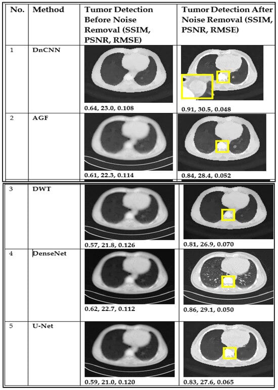
Figure 6.
CT image performance in tumor detection before and after denoising using DnCNN, AGF, U-Net, DWT, and DenseNet. The yellow parts from numbers 1–5 indicate tumorous regions.
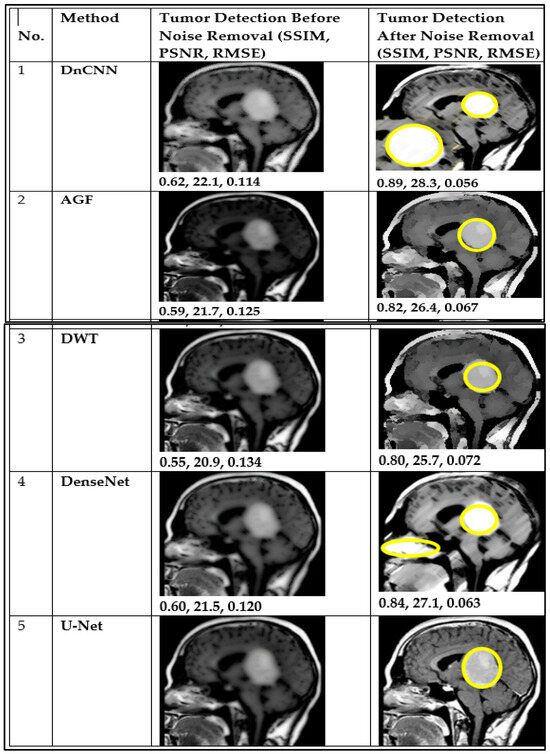
Figure 7.
MRI image performance in tumor detection before and after denoising using DnCNN, GF, U-Net, DWT, and DenseNet. The yellow parts from numbers 1–5 indicate tumorous regions.
Figure 7 presents MRI images that illustrate tumor detection performance before denoising (BDn) and after denoising (ADn) using different methods. The DnCNN demonstrates better performance, achieving higher SSIM and PSNR, along with lower RMSE, compared to other methods. It was closely followed by DenseNet, even though it introduced blurring.
Figure 8 and Figure 9 illustrate the results of CT and MRI image denoising for tumor detection (BDn) and (ADn). The performance in both CT and MRI images indicates improved visual representation after denoising, enhancing the detection of tumors in low-quality images. The DnCNN outperformed other methods based on PSNR (29.5 dB) and SSIM (0.91) for CT images and a PSNR of 28.3 dB and SSIM of 0.89 for MRI images, as shown in Figure 8 and Figure 9 and confirmed in Table 2 and Table 3. The good performance of DnCNN is attributed to its ability to learn from a large dataset of noisy and clean image pairs, enabling it to better preserve important image features while removing noise. It was closely followed by DenseNet and contrasted with the poor output of AGF. Generally, the impact of CT images in Figure 8 was higher than the MRI images in Figure 9. This is attributed to MRI scans having more complex noise characteristics, such as spatially varying noise, which makes it harder for the model to generalize. Table 2 and Table 3 below confirm the results of Figure 8 and Figure 9, with DnCNN outperforming the rest in terms of PSNR, SSIM, and RMSE.
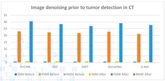
Figure 8.
CT image performance in tumor detection BDn and ADn using DnCNN, AGF, U-Net, DWT, and DenseNet.
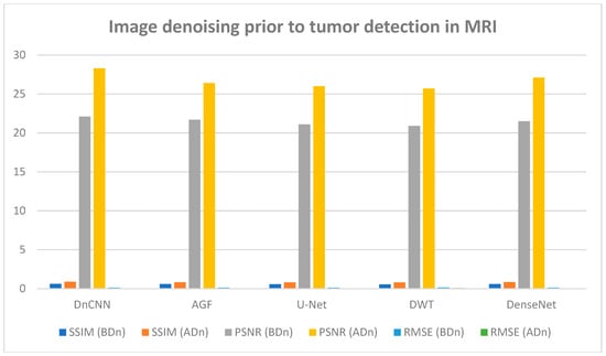
Figure 9.
MRI image performance in tumor detection BDn and ADn using DnCNN, AGF, U-Net, DWT, and DenseNet.
Table 2.
CT performance for tumor detection before denoising (BDn) and after denoising (ADn).
Table 3.
MRI performance for tumor detection before (BDn) and after (ADn) denoising.
The brain CT dataset and brain MRI dataset were used to test the capability of the proposed approach, and results are presented in Tables S1 and S2 and Figure S1.
4.2. Ablation Studies
To gauge the performance of the Adversarial Content–Noise Complementary Learning (ACNCL) denoising model for image denoising and tumor detection, we conducted a comprehensive ablation study on a CT image dataset of lung adenocarcinoma from The Cancer Genome Atlas (TCGA-LUAD) sourced from Kaggle. As shown in Table 4, the analysis compared ACNCL-enhanced networks with baseline models that employed a sole predictor, assessing improvements under different configurations. Specifically, ACNCL-U-Net was compared with the sole U-Net predictor that only focused on content learning and the sole U-Net predictor that only focused on noise learning. The comparative results revealed that ACNCL-U-Net outperformed both baseline models, showcasing its ability to effectively balance content and noise learning for enhanced diagnostics. A broad U-Net with enhanced convolutional layers for content learning and a broad U-Net with enhanced convolutional layers for noise learning were also compared. The findings indicated that the ACNCL-U-Net maintained its outstanding performance, demonstrating a robust architecture that leverages both content and noise features more effectively than the broader U-Net variants. Comparatively, ACNCL-DenseNet was compared with the sole DenseNet predictor focused on content learning and the sole DenseNet predictor focused on noise learning. Additionally, ACNCL-CA-AGF was compared with the sole CA-AGF predictor focused on content learning and the sole CA-AGF predictor focused on noise learning. Separately, the ACNCL-DWT was compared with a sole DWT predictor focused exclusively on content learning and one DWT predictor focused on noise learning. The training followed the same GAN model outlined in Figure 3, except that the generator was adjusted for each network.
Table 4.
Quantitative results (Mean ± SDs) of the ablation study over the CT lung dataset. The ACNCL-U-Net, ACNCL-DnCNN, and ACNCL-DenseNet refer to the proposed ACNCL-based networks whose predictors are two U-nets, two DnCNNs, two DenseNets, two CA-AGFs, and two DWTs.
Table 4 provides quantitative results from an ablation study conducted on a CT dataset, comparing different variations in neural network architectures used for denoising and tumor detection. The key metrics used in this table to assess the efficiency of each model include SSIM, Root MSE, and PSNR. Higher SSIM (Mean ± SD) values indicate better similarity, where a score closer to 1.0 represents a more accurate restoration of the image structure. The RMSE (Mean ± SD) measures the average squared difference between pixel values of the predicted denoised image and the ground truth. Lower RMSE values indicate better performance. Finally, the PSNR represented in decibels (dB, Mean ± SD) is a measure of the ratio between the maximum possible power of a signal and the power of corrupting noise that affects the fidelity of its representation. Higher PSNR values, measured in decibels (dB), indicate better image quality, as less noise is present, signifying accurate tumor detection.
The ACNCL-U-Net is a variation of the U-Net architecture incorporating ACNCL with the highest SSIM and PSNR among all methods. It has the highest SSIM (0.91) and PSNR (30.3 dB) among all the models, indicating it retains the most structure and clarity after denoising, with a relatively low RMSE (0.050), showing accurate restoration and improved tumor detection. Similarly, ACNCL-CA-AGF architecture incorporates Context-Aware-AGF mechanisms with an SSIM of 0.88 and PSNR of 29.9 dB, making it a strong candidate but still lagging behind the ACNCL-U-Net. The ACNCL-DnCNN architecture incorporates ACNCL with an SSIM of 0.86, PSNR of 28.9 dB, and RMSE of 0.056, respectively. It is slightly behind the ACNCL-CA-AGF but still very competitive. The ACNCL-DenseNet model uses the DenseNet architecture combined with ACNCL. It performs well with a high SSIM (0.85) and PSNR (28.1 dB), indicating more effective denoising than ACNCL-DWT with an SSIM value of 0.80 and PSNR of 26.9 dB. It is slightly behind the ACNCL-DnCNN in terms of performance. The results of these comparisons demonstrated that ACNCL models consistently outperformed their single-focus counterparts, highlighting the importance of integrating both content and noise learning for enhanced diagnostic accuracy.
Figure 10 presents the results of the ablation study, whereby impressive analysis was realized when ACNCL-based networks were compared with the sole predictors. For example, a sole DenseNet predictor that only focused on content learning and achieved SSIM 0.80, PSNR 25.7 dB, and RMSE 0.072, and a sole DenseNet predictor that only focused on noise learning and achieved SSIM 0.81, PSNR 26.0 dB, and RMSE 0.070, were compared with ACNCL-DenseNet whose outcome outperformed the single predictors at an SSIM of 0.85, PSNR value of 28.1 dB, and RMSE of 0.058 (Figure 11). The results demonstrated that ACNCL enhances image denoising and tumor detection by using GANs to effectively differentiate between real and noisy images, improving noise removal and preserving fine details for the detection of tumors.
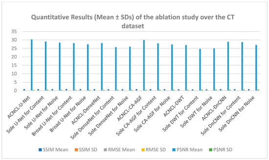
Figure 10.
Quantitative results (Mean ± SDs) representation of the ablation study output of CT lung dataset.
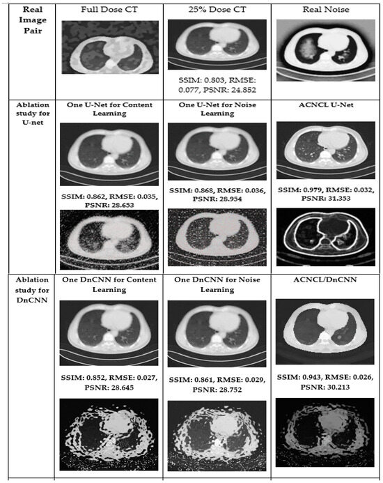
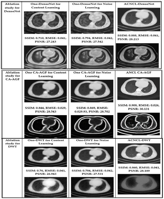
Figure 11.
Visual comparison in the ablation studies on case T430 on CT dataset. The first row is the real image pair. The second and third rows are the ablation study for the situation where the predictor is U-Net. The fourth and fifth rows are the ablation study for DnCNN. The sixth and seventh rows are the ablation study for DenseNet, the eighth and ninth rows are the ablation study for CA-AGF, and lastly, the tenth and eleventh rows are the ablation studies for DWT. Noise images are calculated by subtracting corresponding predicted content images and the real full-dose image.
Comparison with Reference Methods
(a) Results on CT Dataset: For the CT denoising task, we selected BM3D [17], RED-CNN [15], Wasserstein GAN with Gradient Penalty (WGAN-GP) [19], and a variational autoencoder (VAE) [9] as reference methods in the CT denoising tasks. Two representative CT slices containing metastases from patients labeled T521 and T430 are part of the dataset used in the study, which were chosen to visualize the denoising performance of these methods, and the labels T521 and L430 were anonymized to refer to patients in clinical datasets while preserving their privacy. The CT slices are 2D images generated from 3D CT scans, where each slice represents a cross-sectional view of the patient’s anatomy. In this case, the slices specifically contain metastases, which are cancerous growths that have spread from the original tumor to other areas of the body.
In Figure 12, the yellow parts indicate tumorous regions. The BM3D shows blurriness and noise; although the RED-CNN can effectively reduce noise, it tends to overfit the training data, particularly when the dataset lacks diversity. This overfitting leads to poor generalization of unseen data and may introduce noise. The VAE produced denoised images that were blurry. This blurriness was due to the variational approach prioritizing smooth and continuous latent spaces, which can result in the loss of sharp edges and fine details in CT images. The WGAN-GP method excelled in producing high-quality images that retain fine details and textures. This method used Wasserstein distance to provide a smooth and reliable loss function and prevented mode collapse through reducing discriminator dominance for stable training. The gradient penalty was used to prevent training instability by ensuring that medical images remained diverse and realistic. It is obvious that compared with comparison methods, the ACNCL-based networks achieved better denoising outcomes in terms of both content preservation and noise suppression. Among the proposed ACNCL-based networks, ACNCL-U-Net and ACNCL-CA-AGF outperformed ACNCL-DnCNN, ACNCL-DenseNet, and ACNCL-DWT in the aspect of vascular structure preservation.
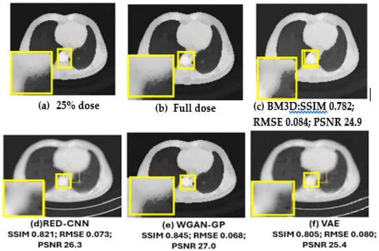
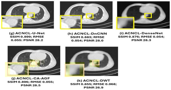
Figure 12.
Comparison of different methods for low-dose CT denoising on case T521. There is a metastatic tumor in the lungs. (a) Full-dose CT; (b) 25% dose CT; (c) BM3D; (d) RED-CNN; (e) WGAN-GP; (f) VAE; (g) ACNCL-U-Net; (h) ACNCL-DnCNN; (i) ACNCL-DenseNet; (j) ACNCL-CA-AGF; (k) ACNCL-DWT. The yellow parts indicate tumorous regions.
Table 5, gives a summary of quantitative results in the whole test set for CT lung datasets. This table shows that ACNCL-U-Net and ACNCL-CA-AGF achieved more efficiency in PSNR and SSIM than ACNCL-DnCNN, ACNCL-DenseNet, and ACNCL-DWT. When compared with comparison methods like the BM3D, RED-CNN, WGAN-GP, and VAE, all the proposed ACNCL-based networks achieved better quantitative outcomes. Similarly, when compared with the results obtained in Table S1 for the brain CT dataset, the outcome had slight deviations, which did not affect the overall performance that reflected ACNCL-based techniques outperforming the single methods. In general, the quantitative evaluation confirmed our visual observations.
Table 5.
Quantitative results (Mean ± SDs) for the low-dose CT lung dataset denoising on the complete test set.
As shown in Figure 13 below, ACNCL-U-Net achieved the best results with an SSIM of 0.899, indicating superior structural similarity, a low RMSE of 0.056, which suggests a minimal error in the denoised image, and a high PSNR of 28.3 dB, reflecting better overall image quality. The next-best-performing model was ACNCL-CA-AGF, which also outperformed all reference methods. In comparison, the best-performing reference model, WGAN-GP, had a lower SSIM of 0.845, a higher RMSE of 0.068, and a PSNR of 27.0 dB. These findings indicate that the ACNCL-based networks are more effective in denoising and preserving key image features than the reference methods. On the other hand, Figure S1 in the Supplementary Material shows that ACNCL-U-Net had the best performance at SSIM of 0.897, RMSE of 0.056, and PSNR of 28.6 db. There was a slight deviation in the SSIM outcome of 0.002, whereby Figure 13 (lung dataset) shows 0.899 and Figure S1 (brain dataset) shows 0.897. PSNR also deviated at 0.3, whereby Figure 13 shows a PSNR of 28.3 dB, and Figure S1 shows 28.6 dB. Although there was a slight deviation in the resultant outcome for SSIM and PSNR values, the general performance revealed that ACNCL-based methods had better results than the single methods for both lung datasets and brain datasets.
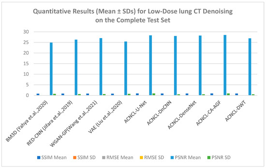
Figure 13.
Quantitative Results (Mean ± SDs) Representation for Low-Dose CT lung Denoising on the Complete Test Set [9,15,17,19].
(b) Results on MRI Dataset: For the MRI dataset, the reference methods included NLM [4], U-Net [11], DnCNN [13], and SCNN [14]. Table 6 shows quantitative results for MRI denoising for full cross-validation.
Table 6.
Quantitative results (Mean ± SDs) for under-sampling MRI denoising on full cross-validation.
As shown in Figure 14 below, the yellow parts indicated tumorous regions identified. All deep learning methods displayed better results, but NLM, while effective at low-to-moderate noise levels, struggled with higher noise levels, leading to over-smoothing of the images. This resulted in the loss of important structural details, especially in areas with subtle contrasts, which is critical for accurate diagnosis. Although the SCNN performed reasonably well, it introduced some noise, which could compromise the diagnostic quality of the images. Both U-Net and DnCNN were effective in noise reduction but at the cost of losing some textural information, which is crucial for accurate diagnosis. The ACNCL-CA-AGF displayed better performance compared to ACNCL-DnCNN and ACNCL-U-NET in image restoration and tumor detection. In general, the proposed ACNCL-based networks were superior to the comparison methods both in noise removal and structural restoration. The quantitative results of the complete cross-validation are provided in Table 6. Compared with the reference methods, the ACNCL-based networks had better performance in terms of all evaluation metrics.
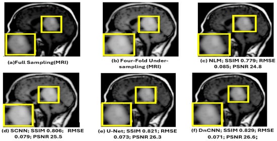
Figure 14.
Comparison of different methods for under-sampling MRI denoising and tumor detection. (a) Full-sampling MRI. (b) Four-fold under-sampling MRI. (c) NLM. (d) SCNN. (e) U-Net. (f) DnCNN. (g) ACNCL-U-Net. (h) ACNCL-DnCNN. (i) ACNCL-DenseNet. (j) ACNCL-CA-AGF. (k) ACNCL-DWT. The yellow parts indicate tumorous regions identified.
The water images and the fat images of the WFI (Water–Fat Imaging) sequence were selected for visual comparison of MRI denoising, as illustrated in Figure 14.
The findings in Figure 15 below reveal that ACNCL-based models outperformed their reference models due to the incorporation of Adversarial Content–Noise Complementary Learning. The ACNCL-DnCNN achieved a higher SSIM value of 0.893, indicating better preservation of structural similarity between the denoised image and the ground truth, as well as a lower RMSE of 0.059, suggesting reduced error in the denoised image. Additionally, it showed a higher PSNR value of 28.1 dB, reflecting better overall image quality compared to the reference DnCNN model, which had an SSIM of 0.829, RMSE of 0.071, and PSNR of 26.6 dB. These improvements suggest that ACNCL enhances the model’s ability to handle noise while maintaining key image features more effectively.
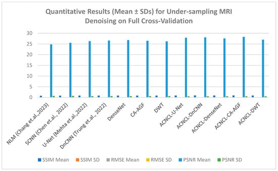
Figure 15.
Quantitative results (Mean ± SDs) for sampling MRI denoising [4,11,13,14].
5. Cross-Contextual Studies
In functional imaging, noise affects the accuracy of quantitative measurements, leading to incorrect clinical interpretations. In cases where there are low-quality medical images, critical diagnoses might be misinterpreted entirely. Therefore, it is necessary to evaluate the generalization capability of a trained ACNCL predictor model. We investigated the universality of the proposed ACNCL-based networks using brain CT dataset object detection for a comparison of the obtained results with those of brain CT images. ACNCL was applied to the human brain CT dataset accessed at this link: https://www.kaggle.com/datasets/trainingdatapro/computed-tomography-ct-of-the-brain/data, accessed on 13 December 2024. The full-dose and 25% dose CT images in the brain CT data were obtained from actual scans.
The experiments represented in Figure 6 (CT lung dataset) and Figure 7 (MRI brain dataset) after denoising revealed that DnCNN had the best achievement based on PSNR, SSIM, and RMSE values compared with DenseNet, AGF, DWT, and U-NET across all CT and MRI datasets. Quantitatively, DnCNN in Table 2 for CT lung images had an SSIM of 0.64 before denoising (BDn) and moved up to an SSIM of 0.91 after denoising (ADn), RMSEs of 0.108 (BDn) and 0.048 (ADn), and finally PSNRs of 23.0 dB (BDn) and 29.5 dB (ADn). On the other hand, as shown in Table S1, the DnCNN using the brain CT dataset had SSIMs of 0.63 (BDn) and 0.90 (ADn), RMSEs of 0.112 (BDn) and 0.054 (ADn), and lastly PSNR values of 22.5 dB (BDn) and 28.7 dB (ADn). The same results for DnCNN’s exceptional outcome over other methods are shown in Table S2 for the brain MRI dataset collected from [26]. Given that WGAN-GP achieved better performance among the reference methods over the CT lung dataset (TCGA-LUAD), as shown in Figure 13 and Table 5, it was compared with the output generated in Figure S1 and Table S1 for the brain CT dataset where WGAN-GP had exceptional PSNR and SSIM compared to the other reference methods. Notable improvement across different datasets for tumor detection after denoising was reported across the four datasets, as shown in Table 2, Table 3, Tables S1 and S2.
The results in Figure 13 and Table 5, put ACNCL-U-Net in the lead with an SSIM of 0.899, PSNR of 28.3 dB, and RMSE of 0.056, and generally, all other ACNCLs remarkably gave better results than all other reference methods. This is supported by the findings of the brain CT dataset in Figure S1, where notable achievements for ACNCL networks were seen compared to the reference methods.
6. Discussion
The quality of medical imaging modalities in clinical diagnosis relies heavily on the production of clean images for the accurate detection of tumors and lesions in CT and MRI images. The low quality of medical images leads to misdiagnosis of diseases. In this study, we propose an Adversarial Content–Noise Complementary Learning (ACNCL) model for image denoising and tumor detection tailored for use in medical imaging. This approach allows simultaneous learning of content and noise, improving both denoising and tumor detection accuracy while mitigating common GAN issues. The ACNCL model integrates image denoising with tumor detection, utilizing predictors like DnCNN, U-Net, DenseNet, DWT, and CA-AGF within a GAN architecture.
From the results of image denoising before tumor detection in CT and MRI shown in Table 2, Table 3, Tables S1 and S2, the images show remarkable improvement in the detection of tumors after image denoising. The findings exhibited in Figure 8 and Figure 9 demonstrate the power of image denoising before tumor detection to improve detection accuracy for better clinical diagnosis. Further to this, an ablation study was performed involving five predictors, namely DnCNN, U-Net, CA-AGF, DenseNet, and DWT, in addition to our ACNCL model, to show the power of our denoising model in improving tumor detection. To evaluate the effectiveness of the Adversarial Content–Noise Complementary Learning (ACNCL) model for image denoising and tumor detection, we compared the ACNCL-based models with their baseline networks comprising DnCNN, CA-AGF, DenseNet, U-Net, and DWT which utilized a single predictor for each case, as shown in Table 4. The results reveal that ACNCL-based networks outperformed the sole predictors for content and noise prediction. For instance, ACNCL-U-Net had the best results across all the metrics used. It had an SSIM value of 0.91, PSNR value of 30.3 dB, and RMSE of 0.050 compared to the sole U-net for content prediction, with an SSIM of 0.88, PSNR of 29.0 dB, and RMSE of 0.055, and the sole U-net for noise prediction, with an SSIM of 0.87, PSNR of 28.4 dB, and RMSE of 0.056. The ACNCL-U-Net performance indicates that it was able to retain the most structures, image clarity, and restoration after denoising. This was followed by ANCL-CA-AGF and ACNCL-DnCNN, which lagged behind ACNCL-U-Net but were competitive and produced better results than ACNCL-DWT. All the sole predictors for noise and content performed dismally compared to the ACNCL-based networks. Figure 11 shows a visual comparison in ablation studies on the CT lung dataset, whereby the ACNCL-based networks subdued the sole predictors in all metrics used. A representative case is where the ACNCL-U-Net had an SSIM value of 0.979, RMSE of 0.032, and PSNR of 31.353 dB compared to the sole predictor for content learning, U-Net, which had an SSIM value of 0.862, RMSE of 0.035, and PSNR of 28.653 dB. Similarly, in Figure 12, for the MRI dataset, the ACNCL-based networks demonstrated superior denoising, excelling in both content preservation and noise reduction. Among these networks, ACNCL-U-Net and ACNCL-CA-AGF outperformed ACNCL-DnCNN, ACNCL-DenseNet, and ACNCL-DWT as they had the highest PSNR values and SSIM values closer to 1. This means that there were better-quality images that evaluated how well features like tumors were preserved after noise reduction. An SSIM value closer to 1 indicates that structural information and the fidelity of tumor shape and texture were preserved. The ACNCL-DnCNN and ACNCL-DenseNet had better RMSE and PSNR compared to ACNCL-DWT, as shown in Table 5, but this came at the cost of some blurring in structural features. When compared with comparison methods like BM3D, RED-CNN, WGAN-GP, and VAE, all the proposed ACNCL-based networks achieved better quantitative results. In general, the quantitative evaluation in Table 5 confirmed our visual observations. Regarding MRI comparison of different methods for under-sampling MRI denoising and tumor detection, the NLM, SCNN, U-Net, and DnCNN were used as reference methods, as shown in Figure 14. All the ACNCL-based networks displayed better results across all metrics used. Non-local means, while effective at low-to-moderate noise levels, were not competent at higher noise levels. The SCNN struggled with non-uniform noise, such as periodic patterns or correlated noise, which required more sophisticated contextual information. Both U-Net and DnCNN were effective in noise reduction but at the cost of blurriness and over-smoothed textures, leading to output that was clean but lacked natural sharpness. The ACNCL-CA-AGF displayed better results compared to ACNCL-DnCNN and ACNCL-U-NET in image restoration and tumor detection, as confirmed in Table 6. In general, the proposed ACNCL-based networks were superior to the comparison methods both in noise removal and structural restoration.
7. Conclusions
The proposed Adversarial Content–Noise Complementary Learning (ACNCL) model demonstrates significant advancements in medical image denoising and tumor detection for CT and MRI images. By utilizing a dual-predictor system, the ACNCL separates content preservation and noise suppression, allowing for optimized performance in both tasks. This approach integrates advanced techniques, including DnCNN for learning noise patterns while preserving anatomical structures, U-Net for spatial localization, ideal for segmenting tumors and preserving fine details, and DenseNet for deep feature extraction, enhancing hierarchical representations for robust noise removal and tumor differentiation, leading to improved accuracy and reliability in clinical diagnostics. The CA-AGF was used for context-aware filtering, and DWT for frequency-domain noise isolation. The quantitative results shown in Table 4 underscore its effectiveness, with the ACNCL-U-Net achieving an SSIM of 0.91, PSNR of 30.3 dB, and RMSE of 0.050 for CT images, surpassing standalone predictors like U-Net, which attained an SSIM of 0.88, PSNR of 29.0 dB, and RMSE of 0.055. Similarly, MRI image results reveal the ACNCL model’s improved results over conventional methods such as NLM and SCNN, which exhibited limitations in handling non-uniform noise and preserving fine details.
The model further demonstrates its robustness through an adversarial learning setup and online tumor image comparison for enhanced diagnostic accuracy. Adversarial learning ensures that denoised images resemble clean references, improving overall image quality and diagnostic reliability. The ablation studies shown in Figure 11 highlight the exceptional output of ACNCL-based networks, with ACNCL-U-Net achieving an SSIM of 0.979, PSNR of 31.353 dB, and RMSE of 0.032, compared to sole U-Net’s SSIM of 0.862, PSNR of 28.653 dB, and RMSE of 0.035. Tumor detection accuracy improved notably after denoising, with clear visibility of tumor boundaries and higher structural fidelity in post-processed images, as demonstrated in Figure 6 and Figure 7. Despite its significant contributions, the ACNCL model faces challenges such as computational complexity and reliance on external databases, which may pose data privacy concerns. Future research could focus on optimizing computational efficiency, improving data security, and expanding the model’s application to other medical imaging modalities to further solidify its clinical impact.
Supplementary Materials
The following supporting information can be downloaded at: https://www.mdpi.com/article/10.3390/signals6020017/s1, Figure S1: Quantitative Results (Mean ± SDs) Representation for Low-Dose brain CT Denoising on the Complete Test Set; Table S1: Brain CT performance for tumor detection Before (BDn) and after (ADn); Table S2: Brain MRI performance for tumor detection Before (BDn) and after (ADn).
Author Contributions
Conceptualization, T.A., methodology, T.A. and R.R., experimentation, T.A., original draft preparation, T.A. and R.R., review and editing, T.A. and G.O., funding acquisition, TA and G.O. All authors have read and agreed to the published version of the manuscript.
Funding
This research received no external funding.
Data Availability Statement
Data are contained within the article.
Conflicts of Interest
The authors declare no conflicts of interest.
References
- Hussain, S.; Mubeen, I.; Ullah, N.; Shah, S.S.U.D.; Khan, B.A.; Zahoor, M.; Ullah, R.; Khan, F.A.; Sultan, M.A. Modern diagnostic imaging technique applications and risk factors in the medical field: A review. BioMed Res. Int. 2022, 2022, 5164970. [Google Scholar]
- Islam, S.M.S.; Nasim, M.A.A.; Hossain, I.; Ullah, D.M.A.; Gupta, D.K.D.; Bhuiyan, M.M.H. Introduction of medical imaging modalities. In Data-Driven Approaches on Medical Imaging; Springer Nature: Cham, Switzerland, 2023; pp. 1–25. [Google Scholar]
- Nazir, N.; Sarwar, A.; Saini, B.S. Recent developments in denoising medical images using deep learning: An overview of models, techniques, and challenges. Micron 2024, 180, 103615. [Google Scholar]
- Chang, L.W.; Liao, J.R. Improving non-local means image denoising by correlation correction. Multidimens. Syst. Signal Process. 2023, 34, 147–162. [Google Scholar]
- Abuya, T.K.; Rimiru, R.M.; Okeyo, G.O. An Image Denoising Technique Using Wavelet-Anisotropic Gaussian Filter-Based Denoising Convolutional Neural Network for CT Images. Appl. Sci. 2023, 13, 12069. [Google Scholar] [CrossRef]
- Ismael, A.A.; Baykara, M. Digital Image Denoising Techniques Based on Multi-Resolution Wavelet Domain with Spatial Filters: A Review. Trait. Signal 2021, 38, 639–651. [Google Scholar] [CrossRef]
- Elad, M.; Kawar, B.; Vaksman, G. Image denoising: The deep learning revolution and beyond—A survey paper. SIAM J. Imaging Sci. 2023, 16, 1594–1654. [Google Scholar] [CrossRef]
- Jakhar, S.P.; Nandal, A.; Dhaka, A.; Alhudhaif, A.; Polat, K. Brain tumor detection with multi-scale fractal feature network and fractal residual learning. Appl. Soft Comput. 2024, 153, 111284. [Google Scholar] [CrossRef]
- Liu, Z.S.; Siu, W.C.; Wang, L.W.; Li, C.T.; Cani, M.P. Unsupervised real image super-resolution via generative variational autoencoder. In Proceedings of the IEEE/CVF Conference on Computer Vision and Pattern Recognition Workshops, Seattle, WA, USA, 14–19 June 2020; pp. 442–443. [Google Scholar]
- Di Feola, F.; Tronchin, L.; Guarrasi, V.; Soda, P. Multi-Scale Texture Loss for CT denoising with GANs. arXiv 2024, arXiv:2403.16640. [Google Scholar]
- Mehta, D.; Padalia, D.; Vora, K.; Mehendale, N. MRI image denoising using U-Net and Image Processing Techniques. In Proceedings of the 2022 5th International Conference on Advances in Science and Technology (ICAST), Mumbai, India, 2–3 December 2022; IEEE: Piscataway, NJ, USA, 2022; pp. 306–313. [Google Scholar]
- Zhang, J.; Zhou, H.; Niu, Y.; Lv, J.; Chen, J.; Cheng, Y. CNN and multi-feature extraction-based denoising of CT images. Biomed. Signal Process. Control 2021, 67, 102545. [Google Scholar] [CrossRef]
- Trung, N.T.; Trinh, D.H.; Trung, N.L.; Luong, M. Low-dose CT image denoising using deep convolutional neural networks with extended receptive fields. Signal Image Video Process. 2022, 16, 1963–1971. [Google Scholar] [CrossRef]
- Chen, Y.; Li, Y.; Zhang, X.; Sun, J.; Jia, J. Focal sparse convolutional networks for 3d object detection. In Proceedings of the IEEE/CVF Conference on Computer Vision and Pattern Recognition, New Orleans, LA, USA, 18–24 June 2022; pp. 5428–5437. [Google Scholar]
- Jifara, W.; Jiang, F.; Rho, S.; Cheng, M.; Liu, S. Medical image denoising using convolutional neural network: A residual learning approach. J. Supercomput. 2019, 75, 704–718. [Google Scholar]
- Geng, M.; Meng, X.; Yu, J.; Zhu, L.; Jin, L.; Jiang, Z.; Qiu, B.; Li, H.; Kong, H.; Yuan, J.; et al. Content-noise complementary learning for medical image denoising. IEEE Trans. Med. Imaging 2021, 41, 407–419. [Google Scholar] [CrossRef]
- Yahya, A.A.; Tan, J.; Su, B.; Hu, M.; Wang, Y.; Liu, K.; Hadi, A.N. BM3D image denoising algorithm based on adaptive filtering. Multimed. Tools Appl. 2020, 79, 20391–20427. [Google Scholar]
- Kim, H.J.; Lee, D. Image denoising with conditional generative adversarial networks (CGAN) in low-dose chest images. Nucl. Instrum. Methods Phys. Res. Sect. A Accel. Spectrometers Detect. Assoc. Equip. 2020, 954, 161914. [Google Scholar]
- Wang, G.; Hu, X. Low-dose CT denoising using a progressive Wasserstein generative adversarial network. Comput. Biol. Med. 2021, 135, 104625. [Google Scholar]
- Yang, Q.; Yan, P.; Zhang, Y.; Yu, H.; Shi, Y.; Mou, X.; Kalra, M.K.; Zhang, Y.; Sun, L.; Wang, G. Low-dose CT image denoising using a generative adversarial network with Wasserstein distance and perceptual loss. IEEE Trans. Med. Imaging 2018, 37, 1348–1357. [Google Scholar]
- Kascenas, A.; Sanchez, P.; Schrempf, P.; Wang, C.; Clackett, W.; Mikhael, S.S.; Voisey, J.P.; Goatman, K.; Weir, A.; Pugeault, N.; et al. The role of noise in denoising models for anomaly detection in medical images. Med. Image Anal. 2023, 90, 102963. [Google Scholar]
- Shomal Zadeh, F.; Pooyan, A.; Alipour, E.; Hosseini, N.; Thurlow, P.C.; Del Grande, F.; Shafiei, M.; Chalian, M. Dynamic contrast-enhanced magnetic resonance imaging (DCE-MRI) in the differentiation of soft tissue sarcoma from benign lesions: A systematic review of the literature. Skelet. Radiol. 2024, 53, 1343–1357. [Google Scholar]
- Xu, X.; Wang, R.; Fu, C.W.; Jia, J. Snr-aware low-light image enhancement. In Proceedings of the IEEE/CVF Conference on Computer Vision and Pattern Recognition, New Orleans, LA, USA, 18–24 June 2022; pp. 17714–17724. [Google Scholar]
- Koonjoo, N.; Zhu, B.; Bagnall, G.C.; Bhutto, D.; Rosen, M.S. Boosting the signal-to-noise of low-field MRI with deep learning image reconstruction. Sci. Rep. 2021, 11, 8248. [Google Scholar]
- Sarkar, K.; Bag, S.; Tripathi, P.C. Noise-aware content-noise complementary GAN with local and global discrimination for low-dose CT denoising. Neurocomputing 2024, 582, 127473. [Google Scholar]
- Tang, Y.; Du, Q.; Wang, J.; Wu, Z.; Li, Y.; Li, M.; Yang, X.; Zheng, J. CCN-CL: A content-noise complementary network with contrastive learning for low-dose computed tomography denoising. Comput. Biol. Med. 2022, 147, 105759. [Google Scholar] [CrossRef]
- Utz, J.; Weise, T.; Schlereth, M.; Wagner, F.; Thies, M.; Gu, M.; Uderhardt, S.; Breininger, K. Focus on Content not Noise: Improving Image Generation for Nuclei Segmentation by Suppressing Steganography in CycleGAN. In Proceedings of the IEEE/CVF International Conference on Computer Vision, Paris, France, 6 October 2023; pp. 3856–3864. [Google Scholar]
- Ghahremani, M.; Khateri, M.; Sierra, A.; Tohka, J. Adversarial distortion learning for medical image denoising. arXiv 2022, arXiv:2204.14100. [Google Scholar]
- Jiang, J.; Wang, Z.; Qiu, S.; Zhang, K.; Su, Y.; Zhang, M.; Zhang, C. Multi-Task Learning-Based Method for Load Identification, Electrical Fault Detection, and Signal Denoising. IEEE Sens. J. 2024, 24, 40069–40082. [Google Scholar] [CrossRef]
- Sun, Y.; Yang, H.; Zhou, J.; Wang, Y. ISSMF: Integrated semantic and spatial information of multi-level features for automatic segmentation in prenatal ultrasound images. Artif. Intell. Med. 2022, 125, 102254. [Google Scholar] [CrossRef]
- Isola, P.; Zhu, J.Y.; Zhou, T.; Efros, A.A. Image-to-image translation with conditional adversarial networks. In Proceedings of the IEEE Conference on Computer Vision and Pattern Recognition, Honolulu, HI, USA, 21–26 July 2017; pp. 1125–1134. [Google Scholar]
- Albertina, B.; Watson, M.; Holback, C.; Jarosz, R.; Kirk, S.; Lee, Y.; Rieger-Christ, K.; Lemmerman, J. The Cancer Genome Atlas Lung Adenocarcinoma Collection (TCGA-LUAD) (Version 4) [Data set]. Cancer Imaging Arch. 2016. [Google Scholar] [CrossRef]
- Grøvik, E.; Yi, D.; Iv, M.; Tong, E.; Rubin, D.; Zaharchuk, G. Deep learning enables automatic detection and segmentation of brain metastases on multisequence MRI. J. Magn. Reson. Imaging 2020, 51, 175–182. [Google Scholar] [CrossRef]
- Prasad, M.A.; Subiramaniyam, N.P. A hybrid approach of Adam optimization with CNN to remove noise on images. In Proceedings of the 2022 International Mobile and Embedded Technology Conference (MECON), Noida, India, 10–11 March 2022; IEEE: Piscataway, NJ, USA, 2022; pp. 527–530. [Google Scholar]
Disclaimer/Publisher’s Note: The statements, opinions and data contained in all publications are solely those of the individual author(s) and contributor(s) and not of MDPI and/or the editor(s). MDPI and/or the editor(s) disclaim responsibility for any injury to people or property resulting from any ideas, methods, instructions or products referred to in the content. |
© 2025 by the authors. Licensee MDPI, Basel, Switzerland. This article is an open access article distributed under the terms and conditions of the Creative Commons Attribution (CC BY) license (https://creativecommons.org/licenses/by/4.0/).