Use RBF as a Sampling Method in Multistart Global Optimization Method

Abstract

In this paper, a new sampling technique is proposed that can be used in the Multistart global optimization technique as well as techniques based on it. The new method takes a limited number of samples from the objective function and then uses them to train an Radial Basis Function (RBF) neural network. Subsequently, several samples were taken from the artificial neural network this time, and those with the smallest network value in them are used in the global optimization method. The proposed technique was applied to a wide range of objective functions from the relevant literature and the results were extremely promising.

1. Introduction

A novel method to draw samples for global optimization methods is presented here. The process of locating the global minimum of a continuous and differentiable function $f:S\to R,S\subset R^n$ is described as, determine

$$x^{*}=\arg \underset{x\in S}{min}f\left(x\right)$$

(1)

with S:

$$S=\left[a_1,b_1\right]\otimes \left[a_2,b_2\right]\otimes \dots \left[a_n,b_n\right]$$

The above problem is commonly used to describe problems in economics [1,2,3], physics [4,5,6], chemistry [7,8,9], medicine [10,11] etc. The global optimization methods have two major categories: deterministic and stochastic methods. The most common methods of the first category are the so-called Interval methods [12,13,14], where the set S is divided iteratively in subregions and some subregions that do not contain the global solution are discarded using some pre-defined criteria. The majority of the methods belong to the second category where the reader can find Controlled Random Search methods [15,16,17], Simulated Annealing methods [18,19], Differential Evolution methods [20,21], Genetic algorithms [22,23,24], Particle Swarm optimization methods [25,26], Ant Colony methods [27,28] etc. Moreover, many hybrid stochastic methods have appeared recently in the relevant literature, such as methods that combine Particle Swarm Optimization and Simulated Annealing [29,30], methods that combine Genetic Algorithms and Differential Evolution [31,32], combinations of Genetic Algorithms and Particle Swarm Optimization [33] etc. Furthermore, due to the wide spread of parallel architectures in recent years as well as the widespread use of Graphics Processing Units (GPU), many methods have emerged that exploit such architectures [34,35,36].

This paper proposes an innovative sampling technique for the Multistart stochastic global sampling method. The Multistart technique is one of the simplest stochastic global optimization techniques and is the basis for many modern global optimization methods. In the Multistart method, a series of random samples are taken from the objective function and then a local optimization method is started from each sample. Regarding its simplicity, the method has been used with success in a wide area of practical applications, such as the Travelling Salesman Problem (TSP) [37,38,39], the vehicle routing problem [40,41], the facility location problem [42], the maximum clique problem [43], the maximum fire risk insured capital problem [44], aerodynamic shape problems [45] etc. In addition, the Multistart method has been thoroughly studied by many researchers in recent years, and many works have been proposed on this method, such as methods for finding all local minima of a function [46,47,48], hybrid techniques [49,50], GRASP methods [51], new termination rules [52,53,54], parallel techniques [55,56]. Usually, in the Multistart method, samples are used from the objective function using some distribution such as the uniform distribution. In the present work, it is proposed that these samples are obtained from an RBF network [57], which has already been trained on a limited number of real samples from the objective function. RBF networks have been widely used in many real world problems, such as face recognition [58], function approximation [59,60], image classification [61], water quality prediction [62] etc.

The proposed sampling methodology generates an approximation of the objective function by first taking some samples from it and then trains a neural network to approximate the function. Once the neural network training process is completed, a bunch of points can be sampled from the neural network and those with the lowest functional value will be used as starting points for the Multistart method. This way, the actual function will not be sampled but the neural network approximating it, which should significantly reduce the required number of function calls. Furthermore, using points with a low function value as starting points is expected to speed up the location of the global minimum. In addition, the RBF neural network is incorporated since it has a very fast training technique.

The rest of this article is organized as follows: in Section 2 the proposed sampling technique is outlined in detail, in Section 3 the test functions used as well the experimental results are listed and finally in Section 4 some conclusions are presented.

2. Method Description

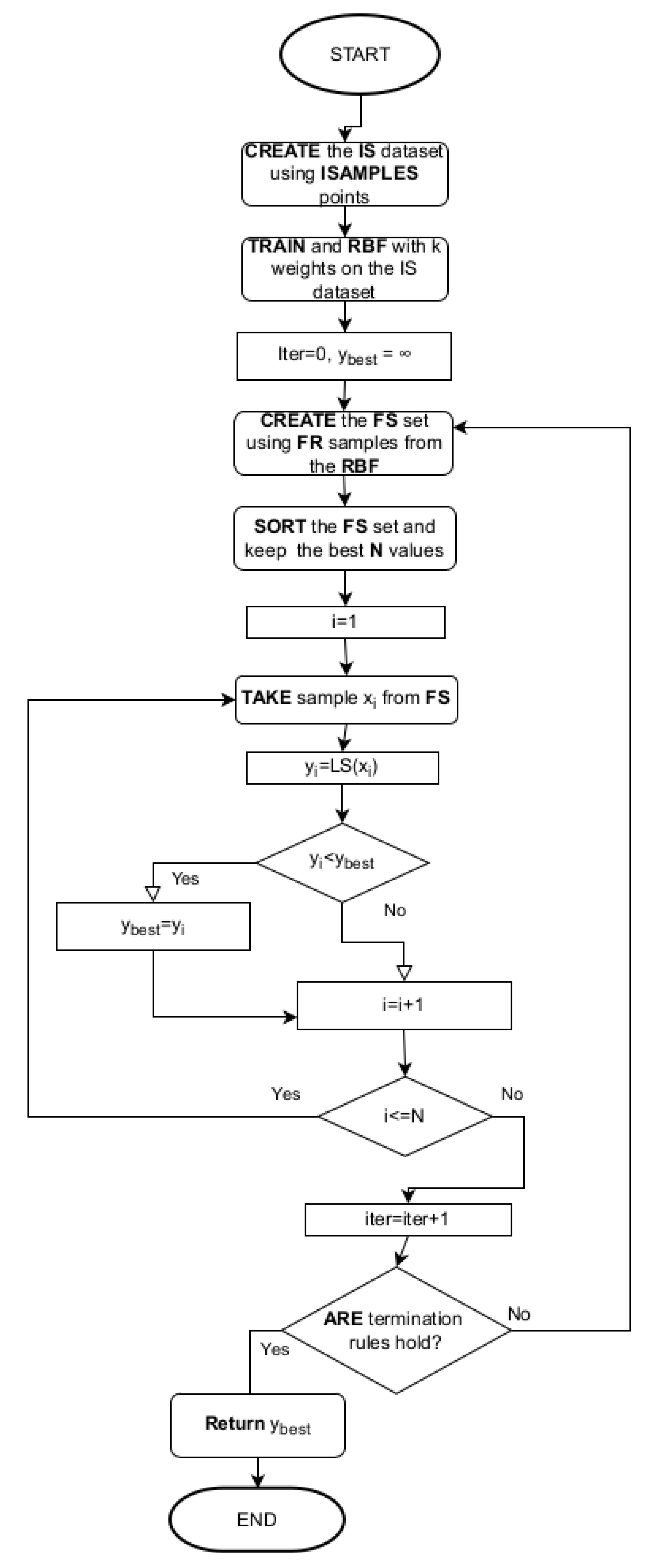
2.1. The Multistart Method

A commonly used representation of the Multistart method is shown in Algorithm 1. In practice, the method takes N samples at each iteration and starts a local minimization method for each sample, without doing any other checking. However, despite its simplicity, it has two key components which, with proper adaptation, can make the method extremely efficient. The first component is the termination method used and the second is the sampling method within the central iteration. The local search procedure used here is an adaptation of the Broyden–Fletcher–Goldfarb–Shanno (BFGS) method [63]. The used termination rule was also used in a variety of global optimization methods [64,65]. This termination method is outlined in Section 2.2 The second point, which this paper focuses on, is the sampling method. Usually, sampling is performed with random samples from some distribution such as the uniform one. In this paper, samples will be taken from an approximation of the objective function $f\left(x\right)$ constructed using an RBF neural network. This approach is discussed in Section 2.3.

Algorithm 1 Representation of the Multistart algorithm.

Initialization step. (a) Set N the number of samples, that will taken in every iteration. (b) Set ${\mathrm{ITER}}_{\mathrm{MAX}}$, the maximum number of allowed iterations. (c) Set Iter = 0, the iteration number. (d) Set $\left(x^{*},y^{*}\right)$ as the global minimum. Initially $y^{*}=\infty$ Evaluation step. (a) Set Iter=Iter+1 (b) For $i=1\dots N$ Do i. Take a new sample $x_i\in S$ ii. $y_i=\mathrm{LS}\left(x_i\right)$. Where LS(x) is a predefined local search method. iii. If $y_i\le y^{*}$ then $x^{*}=x_i,y^{*}=y_i$ (c) EndFor Termination check. The termination criteria are checked and if they are true, then the method terminates.

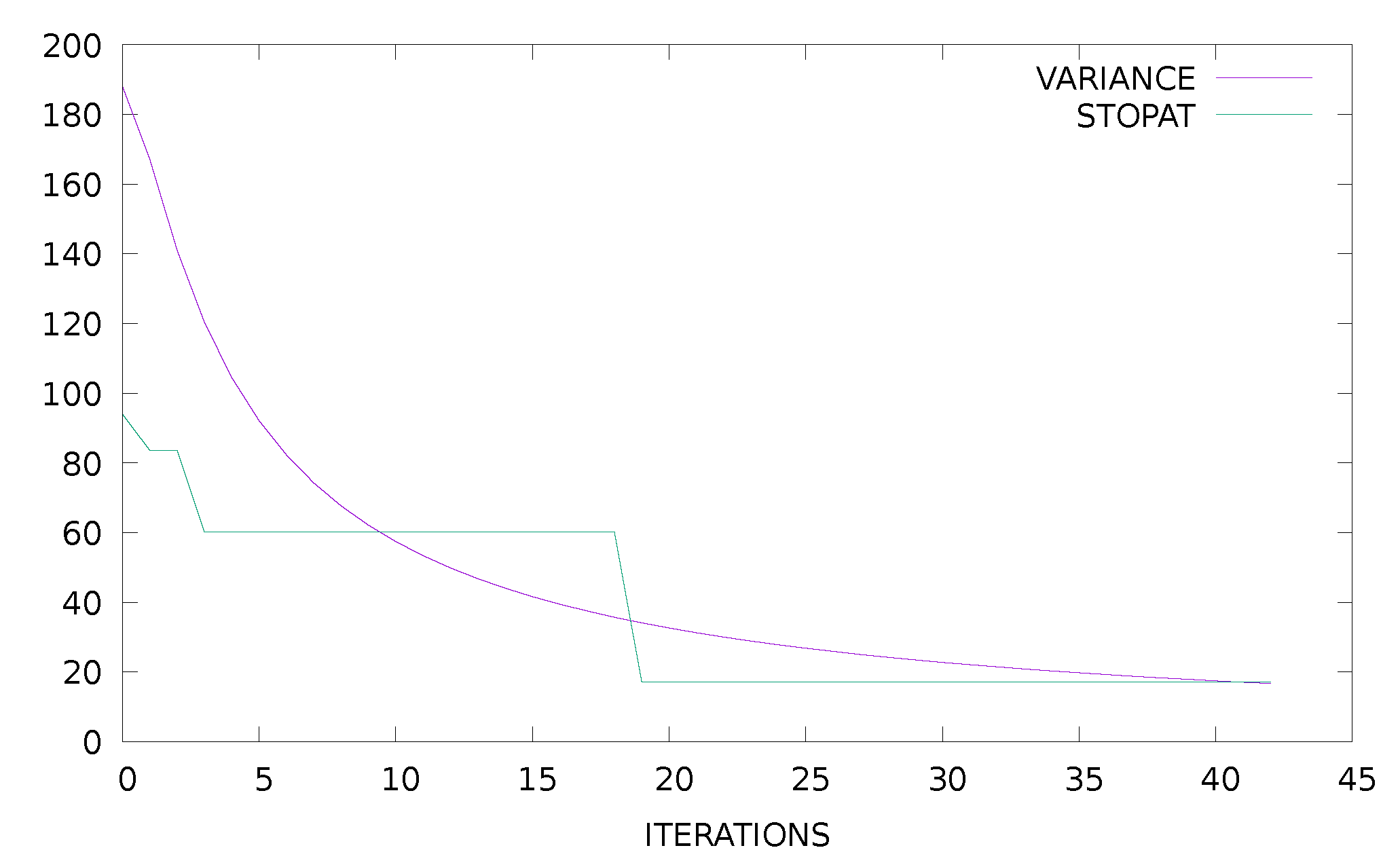
2.2. The Used Termination Rule

A typical termination method used is the maximum number of iterations, i.e., to terminate the method when $\mathrm{Iter}\ge {\mathrm{ITER}}_{\mathrm{MAC}}$. However, this way of termination is not particularly efficient, since for small values of the ${\mathrm{ITER}}_{\mathrm{MAC}}$ number the total minimum may not be found, while for larger values of it it may be found at an early stage of the search and then the computer wastes time on calls of local search method. As an example, consider the Hansen function, defined as:

$$f\left(x\right)=\sum _{i=1}^{5}icos\left[(i-1)x_1+i\right]\sum _{j=1}^{5}jcos\left[(j+1)x_2+j\right],x\in {[-10,10]}^2$$

The global minimum for the function is −176.541793. The progress of solving the above function with ${\mathrm{ITER}}_{\mathrm{MAC}}=100$ is shown in Figure 1. The global minimum was discovered too early, at the 21th iteration, but the algorithm continues until Iter = 100, spending 80% of computing time. The termination rule used in this work was first proposed in [64]: at every iteration n the variance of the quantity $f\left(x^{*}\right)$ is calculated. This quantity is denoted as $v^{\left(n\right)}$. If the variance falls below a predetermined threshold, then the method is terminated. This limit is half the value of this variance for the last time a new low was found for $y^{*}$. The algorithm terminates when

$$v^{\left(n\right)}\le \frac{v^{\left(\mathrm{nlast}\right)}}{2}$$

(2)

where nlast is the last iteration where a new better estimation of the global minimum was discovered. A graphical representation for the proposed method and the function EXP8 is shown in Figure 2. The value $v^{\left(n\right)}$ is denoted as VARIANCE in the plot and the value $\frac{v^{\left(\mathrm{nlast}\right)}}{2}$ is denoted as STOPAT. The function EXP8 is given by

$$f\left(x\right)=-exp\left(-0.5\sum _{i=1}^8{x}_i^2\right),-1\le x_i\le 1$$

The method now terminates at generation 12.

2.3. RBF Networks

An RBF neural network typically is expressed as a function:

$$y\left(\overrightarrow{x}\right)=\sum _{i=1}^k{w}_i\varphi \left(∥x-c_i∥\right)$$

(3)

where the vector $\overrightarrow{x}$ stands for the input vector of the network and the vector $\overrightarrow{w}$ is called weight vector with k elements. Typically, the function $\varphi \left(x\right)$ is the so-called Gaussian function defined as:

$$\varphi \left(x\right)=exp\left(-\frac{{\left(x-c\right)}^2}{{\sigma }^2}\right)$$

(4)

where the value $\varphi \left(x\right)$ depends mainly on the distance between x and x. The vector $\overrightarrow{c}$ is called centroid and the vector $\overrightarrow{\sigma }=\left({\sigma }_1,{\sigma }_2,\dots ,{\sigma }_k\right)$ is considered as the variance vector. A typical plot of this function is shown in Figure 3.

The network of Equation (3) can be used to approximate functions $f\left(x\right),x\in S\subset R^n$ by minimizing the error:

$$E\left(y\left(\overrightarrow{x}\right)\right)=\sum _{i=1}^M{\left(y\left(x_i\right)-f\left(x_i\right)\right)}^2$$

(5)

where the variable M denotes the number of training samples provided for the function $f\left(x\right)$. The RBF network is shown graphically in Figure 4. During a training procedure, the parameters of the RBF network are adapted in order to minimize the error of Equation (5). The RBF network us trained using a two-phase methodology:

• During the first phase the k centers of and the associated variances are calculated through K-Means algorithm [66].
• During the second phase, the weight vector $\overrightarrow{w}=\left(w_1,w_2,\dots ,w_k\right)$ is calculated by solving a linear system of equations with the following procedure:

  (a)

  Set $W=w_{kj}$, the matrix for the k weights

  (b)

  Set $\mathsf{\Phi }={\varphi }_j\left(x_i\right)$

  (c)

  Set $T=\left\{t_i=f\left(x_i\right),i=1,..,M\right\}$.

  (d)

  The system to be solved is defined as:

  $${\mathsf{\Phi }}^T\left(T-\mathsf{\Phi }{W}^T\right)=0$$

  (6)

  The solution is:

  $$W^T={\left({\mathsf{\Phi }}^T\mathsf{\Phi }\right)}^{-1}{\mathsf{\Phi }}^{T}T={\mathsf{\Phi }}^{†}T$$

  (7)

  The matrix ${\mathsf{\Phi }}^{†}={\left({\mathsf{\Phi }}^T\mathsf{\Phi }\right)}^{-1}{\mathsf{\Phi }}^T$ is the so - called pseudo-inverse of $\mathsf{\Phi }$, with the property

  $${\mathsf{\Phi }}^{†}\mathsf{\Phi }=I$$

  (8)

In the proposed technique, the previously defined network constructs an approximation of the objective function $f\left(x\right)$ and subsequently the method Multistart takes samples from the approximation of the objective function. The process starts by taking some samples from the actual $f\left(x\right)$ function. These samples are then used to train an RBF neural network. After training, many samples are taken from the neural network function and the best ones will be used in the global optimization method. The overall sampling procedure is shown in Algorithm 2.

The overall algorithm is graphically represented in Figure 5 in the form of a flowchart.

Algorithm 2 The proposed sampling procedure.

Initialization step. (a) Set N, the number of required samples. (b) Set ISAMPLES, the initial samples that will be drawn from the function $f\left(x\right)$. (c) Set $\mathrm{FR}$ a real number, with $\mathrm{FR}>N$. For example, $\mathrm{FR}=10\times N$ (d) Set $\mathrm{IS}=\varnothing$ (e) Set $\mathrm{FS}=\varnothing$. This is the final outcome of the algorithm. (f) Set k, the number of weights for the RBF network, Initial Sampling step. (a) For $i=1,\dots ,\mathrm{ISAMPLES}$ do i. Take a sample $s_i=\left(x_i,f\left(x_i\right)\right),x_i\in S\subset R^n$ ii. $\mathrm{IS}=\mathrm{IS}\cup s_i$ (b) End For Training step. (a) Construct an RBF network $y\left(x\right)$ with k weights. (b) Train $y\left(x\right)$ using the set $\mathrm{IS}$ by minimizing the train error of Equation (5). Final sampling step. (a) For $i=1,\dots ,\mathrm{FR}$ do i. Take a sample $s_i=\left(x_i,y\left(x_i\right)\right)$ ii. $\mathrm{FS}=\mathrm{FS}\cup s_i$ (b) End For (c) Sort FS according to the function values. (d) Keep in the set only the N samples with the lowest functional value.

3. Experiments

The effectiveness of the proposed method was evaluated using some benchmark functions from the relevant literature [67,68].

3.1. Test Functions

• Bent Cigar function The function is

  $$f\left(x\right)=x_1^2+{10}^6\sum _{i=2}^n{x}_i^2$$

  with the global minimum $f\left(x^{*}\right)=0$. For the conducted experiments the value $n=10$ was used.
• Bf1 function. The function Bohachevsky 1 is given by the equation

  $$f\left(x\right)=x_1^2+2x_2^2-\frac{3}{10}cos\left(3\pi x_1\right)-\frac{4}{10}cos\left(4\pi x_2\right)+\frac{7}{10}$$

  with $x\in {[-100,100]}^2$. The value of the global minimum is 0.0.
• Bf2 function. The function Bohachevsky 2 is given by the equation

  $$f\left(x\right)=x_1^2+2x_2^2-\frac{3}{10}cos\left(3\pi x_1\right)cos\left(4\pi x_2\right)+\frac{3}{10}$$

  with $x\in {[-50,50]}^2$. The value of the global minimum is 0.0.
• Branin function. The function is defined by $f\left(x\right)={\left(x_2-\frac{5.1}{4{\pi }^2}{x}_1^2+\frac{5}{\pi }{x}_1-6\right)}^2+10\left(1-\frac{1}{8\pi }\right)cos\left(x_1\right)+10$ with $-5\le x_1\le 10,0\le x_2\le 15$. The value of the global minimum is 0.397887.with $x\in {[-10,10]}^2$. The value of the global minimum is −0.352386.
• CM function. The Cosine Mixture function is given by the equation

  $$f\left(x\right)=\sum _{i=1}^n{x}_i^2-\frac{1}{10}\sum _{i=1}^{n}cos\left(5\pi x_i\right)$$

  with $x\in {[-1,1]}^n$. The value of the global minimum is −0.4 and in our experiments we have used $n=4$. The corresponding function is denoted as CM4
• Camel function. The function is given by

  $$f\left(x\right)=4x_1^2-2.1x_1^4+\frac{1}{3}{x}_1^6+x_1{x}_2-4x_2^2+4x_2^4,x\in {[-5,5]}^2$$
  The global minimum has the value of $f\left(x^{*}\right)=-1.0316$
• Discus function. The function is defined as

  $$f\left(x\right)={10}^6{x}_1^2+\sum _{i=2}^n{x}_i^2$$

  with global minimum $f\left(x^{*}\right)=0.$ For the conducted experiments the value $n=10$ was used.
• Easom function. The function is given by the equation

  $$f\left(x\right)=-cos\left(x_1\right)cos\left(x_2\right)exp\left({\left(x_2-\pi \right)}^2-{\left(x_1-\pi \right)}^2\right)$$

  with $x\in {[-100,100]}^2$ and global minimum −1.0
• Exponential function. The function is given by

  $$f\left(x\right)=-exp\left(-0.5\sum _{i=1}^n{x}_i^2\right),-1\le x_i\le 1$$
  The global minimum is located at $x^{*}=(0,0,\dots ,0)$ with value $-1$. In our experiments we used this function with $n=4,16,64$ and the corresponding functions are denoted by the labels EXP4, EXP16, EXP64.
• Griewank2 function. The function is given by

  $$f\left(x\right)=1+\frac{1}{200}\sum _{i=1}^2{x}_i^2-\prod _{i=1}^2\frac{cos\left(x_i\right)}{\sqrt{\left(i\right)}},x\in {[-100,100]}^2$$
  The global minimum is located at the $x^{*}=(0,0,\dots ,0)$ with value 0.
• Griewank10 function. The function is given by the equation

  $$f\left(x\right)=\sum _{i=1}^n\frac{x_i^2}{4000}-\prod _{i=1}^{n}cos\left(\frac{x_i}{\sqrt{i}}\right)+1$$
  In our experiments we have used $n=10$ and the global minimum is 0.0. The function has several local minima in the specified range.
• Hansen function. $f\left(x\right)={\sum }_{i=1}^{5}icos\left[(i-1)x_1+i\right]{\sum }_{j=1}^{5}jcos\left[(j+1)x_2+j\right]$, $x\in {[-10,10]}^2$. The global minimum of the function is −176.541793.
• Hartman 3 function. The function is given by

  $$f\left(x\right)=-\sum _{i=1}^4{c}_{i}exp\left(-\sum _{j=1}^3{a}_{ij}{\left(x_j-p_{ij}\right)}^2\right)$$

  with $x\in {[0,1]}^3$ and $a=\left(\begin{array}{ccc}3& 10& 30\\ 0.1& 10& 35\\ 3& 10& 30\\ 0.1& 10& 35\end{array}\right),c=\left(\begin{array}{c}1\\ 1.2\\ 3\\ 3.2\end{array}\right)$ and

  $$p=\left(\begin{array}{ccc}0.3689& 0.117& 0.2673\\ 0.4699& 0.4387& 0.747\\ 0.1091& 0.8732& 0.5547\\ 0.03815& 0.5743& 0.8828\end{array}\right)$$
  The value of the global minimum is −3.862782.
• Hartman 6 function.

  $$f\left(x\right)=-\sum _{i=1}^4{c}_{i}exp\left(-\sum _{j=1}^6{a}_{ij}{\left(x_j-p_{ij}\right)}^2\right)$$

  with $x\in {[0,1]}^6$ and $a=\left(\begin{array}{cccccc}10& 3& 17& 3.5& 1.7& 8\\ 0.05& 10& 17& 0.1& 8& 14\\ 3& 3.5& 1.7& 10& 17& 8\\ 17& 8& 0.05& 10& 0.1& 14\end{array}\right),c=\left(\begin{array}{c}1\\ 1.2\\ 3\\ 3.2\end{array}\right)$ and

  $$p=\left(\begin{array}{cccccc}0.1312& 0.1696& 0.5569& 0.0124& 0.8283& 0.5886\\ 0.2329& 0.4135& 0.8307& 0.3736& 0.1004& 0.9991\\ 0.2348& 0.1451& 0.3522& 0.2883& 0.3047& 0.6650\\ 0.4047& 0.8828& 0.8732& 0.5743& 0.1091& 0.0381\end{array}\right)$$

  the value of the global minimum is −3.322368.
• High Conditioned Elliptic function, defined as

  $$f\left(x\right)=\sum _{i=1}^n{\left({10}^6\right)}^{\frac{i-1}{n-1}}{x}_i^2$$

  with global minimum $f\left(x^{*}\right)=0$ and the value $n=10$ was used in the conducted experiments
• Potential function. The molecular conformation corresponding to the global minimum of the energy of N atoms interacting via the Lennard-Jones potential [69] is used as a test case here. The function to be minimized is given by:

  $$V_{LJ}\left(r\right)=4ϵ\left[{\left(\frac{\sigma }{r}\right)}^{12}-{\left(\frac{\sigma }{r}\right)}^6\right]$$

  (9)
  In the current experiments two different cases were studied: $n=3,5$
• Rastrigin function. The function is given by

  $$f\left(x\right)=x_1^2+x_2^2-cos\left(18x_1\right)-cos\left(18x_2\right),x\in {[-1,1]}^2$$
  The global minimum is located at $x^{*}=(0,0)$ with value −2.0.
• Shekel 7 function.

  $$f\left(x\right)=-\sum _{i=1}^7\frac{1}{(x-a_i){(x-a_i)}^T+c_i}$$

  with $x\in {[0,10]}^4$ and $a=\left(\begin{array}{cccc}4& 4& 4& 4\\ 1& 1& 1& 1\\ 8& 8& 8& 8\\ 6& 6& 6& 6\\ 3& 7& 3& 7\\ 2& 9& 2& 9\\ 5& 3& 5& 3\end{array}\right),c=\left(\begin{array}{c}0.1\\ 0.2\\ 0.2\\ 0.4\\ 0.4\\ 0.6\\ 0.3\end{array}\right)$. The value of the global minimum is −10.342378.
• Shekel 5 function.

  $$f\left(x\right)=-\sum _{i=1}^5\frac{1}{(x-a_i){(x-a_i)}^T+c_i}$$

  with $x\in {[0,10]}^4$ and $a=\left(\begin{array}{cccc}4& 4& 4& 4\\ 1& 1& 1& 1\\ 8& 8& 8& 8\\ 6& 6& 6& 6\\ 3& 7& 3& 7\end{array}\right),c=\left(\begin{array}{c}0.1\\ 0.2\\ 0.2\\ 0.4\\ 0.4\end{array}\right)$. The value of the global minimum is −10.107749.
• Shekel 10 function.

  $$f\left(x\right)=-\sum _{i=1}^{10}\frac{1}{(x-a_i){(x-a_i)}^T+c_i}$$

  with $x\in {[0,10]}^4$ and $a=\left(\begin{array}{cccc}4& 4& 4& 4\\ 1& 1& 1& 1\\ 8& 8& 8& 8\\ 6& 6& 6& 6\\ 3& 7& 3& 7\\ 2& 9& 2& 9\\ 5& 5& 3& 3\\ 8& 1& 8& 1\\ 6& 2& 6& 2\\ 7& 3.6& 7& 3.6\end{array}\right),c=\left(\begin{array}{c}0.1\\ 0.2\\ 0.2\\ 0.4\\ 0.4\\ 0.6\\ 0.3\\ 0.7\\ 0.5\\ 0.6\end{array}\right)$. The value of the global minimum is −10.536410.
• Sinusoidal function. The function is given by

  $$f\left(x\right)=-\left(2.5\prod _{i=1}^{n}sin\left(x_i-z\right)+\prod _{i=1}^{n}sin\left(5\left(x_i-z\right)\right)\right),0\le x_i\le \pi .$$
  The global minimum is located at $x^{*}=(2.09435,2.09435,\dots ,2.09435)$ with $f\left(x^{*}\right)=-3.5$. In our experiments we used $n=4,8,16$ and $z=\frac{\pi }{6}$ and the corresponding functions are denoted by the labels SINU4, SINU8 and SINU16 respectively.
• Test2N function. This function is given by the equation

  $$f\left(x\right)=\frac{1}{2}\sum _{i=1}^n{x}_i^4-16x_i^2+5x_i,x_i\in [-5,5].$$
  The function has $2^n$ in the specified range and in our experiments we used $n=4,5,6,7$. The corresponding values of the global minimum is −156.664663 for $n=4$, −195.830829 for $n=5$, −234.996994 for $n=6$ and −274.163160 for $n=7$.
• Test30N function. This function is given by

  $$f\left(x\right)=\frac{1}{10}{sin}^2\left(3\pi x_1\right)\sum _{i=2}^{n-1}\left({\left(x_i-1\right)}^2\left(1+{sin}^2\left(3\pi x_{i+1}\right)\right)\right)+{\left(x_n-1\right)}^2\left(1+{sin}^2\left(2\pi x_n\right)\right)$$

  with $x\in [-10,10]$. The function has ${30}^n$ local minima in the specified range and we used $n=3,4$ in our experiments. The value of the global minimum for this function is 0.0.

3.2. Experimental Results

The proposed sampling method was tested against the uniform sampling, for the Multistart global optimization technique. The uniform distribution used to sample points is defined as:

$$x_i=a_i+r\times \left(b_i-a_i\right),i=1\dots n$$

(10)

with $r\in [0,1]$ a random number. The parameters for the experiments are listed in

Table 1. Parameters for the experiments.

PARAMETER	VALUE
${\mathrm{ITER}}_{\mathrm{MAX}}$	100
k	10
N	20,50
FR	$10\times N$

. All the experiments were executed 30 times with different random numbers each time. In all cases, the stopping rule of Section 2.2 was incorporated. The random number function used was the drand48() function of the C programming language. The used software was implemented using the OPTIMUS global optimization environment freely available from https://github.com/itsoulos/OPTIMUS (accessed on 27 November 2022). All the experiments were conducted on an AMD Ryzen 5950X equipped with 128 GB of RAM. The operating system used was Debian Linux and all the programs are compiled using the GNU C++ compiler. The experimental results for used test functions are listed in

Table 2. Experimental results for the Multistart method, using uniform distribution for the samples as defined in Equation (10).

FUNCTION	N = 20	N = 50
BF1	3004	5975
BF2	2828	5826
BRANIN	2409	5415
CAMEL	2661	5599
CIGAR	5588	8410
CM4	3551 (0.87)	6431 (0.80)
DISCUS	2817	5965
EASOM	2204	5202
EXP4	2769	5772
EXP16	2836	5837
EXP64	2912	5914
GRIEWANK2	3938 (0.40)	6572 (0.30)
GRIEWANK10	4536 (0.97)	7520
POTENTIAL3	3121	6120
POTENTIAL5	4363	7320
HANSEN	5344 (0.93)	9536 (0.90)
HARTMAN3	2618	5608
HARTMAN6	3014	6037
HIGHELLIPTIC	4398	7306
RASTRIGIN	3850 (0.83)	6401 (0.77)
ROSENBROCK4	6456	8584
ROSENBROCK8	7646	10095
SHEKEL5	3144	6215
SHEKEL7	3354	6508
SHEKEL10	3388	6860
SINU4	3935	6670 (0.97)
SINU8	5547	8056
SINU16	19,313	35,751 (0.97)
TEST2N4	3035 (0.87)	6002 (0.97)
TEST2N5	3127 (0.73)	6042 (0.67)
TEST2N6	3393 (0.40)	6169 (0.47)
TEST2N7	4075 (0.37)	6443 (0.33)
TEST30N3	3723	6322
TEST30N4	3736	6465
TOTAL	142,632 (0.923)	254,988 (0.916)

,

Table 3. Experimental results for the proposed method with N = 20.

FUNCTION	ISAMPLES = 100	ISAMPLES = 200	ISAMPLES = 500
BF1	1086	1159	1500
BF2	922	1026	1304
BRANIN	503	590	899
CAMEL	670	756	1060
CIGAR	3482	3236	2849
CM4	1583 (0.83)	1716 (0.83)	1861 (0.90)
DISCUS	931	1206	1525
EASOM	1063	401	704
EXP4	766	803	1049
EXP16	912	1009	1303
EXP64	968	1070	1359
GRIEWANK2	2409 (0.53)	1641 (0.40)	2069 (0.57)
GRIEWANK10	2607 (0.97)	2609	2902 (0.93)
POTENTIAL3	1211	1297	1613
POTENTIAL5	2414	2521	2835
HANSEN	6079 (0.87)	4785 (0.83)	6504 (0.77)
HARTMAN3	729	830	1143
HARTMAN6	1111 (0.90)	1290 (0.93)	1525 (0.97)
HIGHELLIPTIC	2618	2671	3098
RASTRIGIN	1727 (0.57)	1043 (0.87)	1386
ROSENBROCK4	4111	2672	4357
ROSENBROCK8	5417	6253	5609
SHEKEL5	1751 (0.73)	2152 (0.90)	1245 (0.90)
SHEKEL7	1667 (0.87)	1627 (0.83)	1676 (0.93)
SHEKEL10	2329 (0.80)	2946 (0.73)	3678 (0.77)
SINU4	938	991	1227
SINU8	1194	1360	1479
SINU16	14,305 (0.87)	32,647 (0.97)	21,363 (0.97)
TEST2N4	904 (0.57)	936 (0.73)	1227
TEST2N5	1881 (0.80)	1218	1351
TEST2N6	1092 (0.67)	1224 (0.87)	1435 (0.97)
TEST2N7	1452 (0.70)	1397 (0.80)	1477 (0.90)
TEST30N3	1244	2054	2584
TEST30N4	2027	2644	2638
TOTAL	74,103 (0.902)	91,780 (0.932)	89,834 (0.958)

and

Table 4. Experimental results for the proposed method with N = 50.

FUNCTION	ISAMPLES = 100	ISAMPLES = 200	ISAMPLES = 500
BF1	1093	1175	1527
BF2	943	1022	1319
BRANIN	502 (0.97)	594	900
CAMEL	642	729	1046
CIGAR	3527	3228	6729
CM4	1491 (0.87)	1884 (0.90)	1799 (0.97)
DISCUS	828	1365	1215
EASOM	2320	398	723
EXP4	766	827	1050
EXP16	912	1007	1298
EXP64	983	1064	1358
GRIEWANK2	1788 (0.50)	1762 (0.43)	2345 (0.50)
GRIEWANK10	2505	2677	2868
POTENTIAL3	1244	1313	1609
POTENTIAL5	2420	2502	2795
HANSEN	6711 (0.70)	4278 (0.70)	7264 (0.67)
HARTMAN3	728	830	1144
HARTMAN6	1027 (0.93)	1202 (0.93)	1492
HIGHELLIPTIC	3455	2889	3078
RASTRIGIN	977 (0.53)	1269 (0.77)	1397 (0.97)
ROSENBROCK4	2348	2453	3278
ROSENBROCK8	3928	4461	4865
SHEKEL5	5630 (0.67)	7498 (0.87)	1510 (0.93)
SHEKEL7	2135 (0.67)	1973 (0.67)	1815 (0.97)
SHEKEL10	1864 (0.73)	1245 (0.60)	3165 (0.83)
SINU4	984	1020	1355
SINU8	10,502	1517	1456
SINU16	95,225 (0.83)	21,658 (0.90)	21,330 (0.87)
TEST2N4	820 (0.63)	1079 (0.90)	1274
TEST2N5	1140 (0.67)	1107 (0.80)	1333
TEST2N6	1203 (0.73)	1371 (0.97)	1440 (0.97)
TEST2N7	1602 (0.50)	1200 (0.77)	1618 (0.97)
TEST30N3	1494	1903	2279
TEST30N4	1164	2287	2284
TOTAL	164,901 (0.880)	82,787 (0.918)	91,958 (0.960)

. The number in the cells denotes the average function calls for the 30 independent runs. The fraction in parentheses stands for the fraction of runs where the global optimum was found. If this number is missing then the global minimum was discovered in every independent run (100% success). At the end of each table, an additional line named total has been added, representing the total number of function calls and, in parentheses, the average success rate in finding the total minimum.

From the experimental results, it follows in principle that the use of neural networks significantly reduces the required number of function calls needed to find the total minimum. This reduction is proportional to the objective function and can reach up to 60% of the original number of function calls. In addition, the usage of the ISAMPLES parameter significantly increases the reliability of the new sampling method. For example, in the case where N = 20 there is an increase in the average success rate for finding the total minimum from 90% to approximately 96%. However, improving the reliability of the method does not imply an increase in the number of function calls. For example, for N = 20 the calls are in the interval $[75,000\dots 90,000]$ without showing any clear increase. However, the use of the new sampling technique requires significantly more computing time than the uniform distribution because of the need to train the RBF networks and also because of the classification that precedes taking the final samples. This difference is demonstrated in Figure 6. In this we see the significant difference in running time for the SINU problem with a different number of dimensions each time.

4. Conclusions

In this paper, an innovative sampling technique was proposed for the Multistart global optimization method. The new technique improves on using a limited number of samples from the objective function in order to construct an estimator of the function. The estimator in the present work was an RBF neural network. After the neural network is trained, a large number of samples are taken from the estimator without using the objective function anymore. Of these samples, only those with the lowest functional value of the estimator are used by the global optimization method. From the experiments performed on a wide range of objective functions, many of which had a large number of dimensions, it appears that the proposed technique significantly outperforms the traditionally used uniform sampling. The gain in the number of calls in many cases exceeds 60%. Nevertheless, the new technique requires more computational time than the uniform distribution, since it is required to train the network as well as to classify a series of samples from it. However, this increase in time could be significantly reduced with the potential use of parallel computing techniques to train neural networks. Moreover, in large computational problems, where the cost of evaluating the objective function is extremely large, the training time of a neural network will be almost negligible. Future research may include:

• Application of the proposed technique to other more efficient global optimization methods.
• Parallelization of the training method for the neural network.
• Usage of more efficient methods to train the RBF networks such as Genetic Algorithms.

References

- Cheong, D.; Kim, Y.M.; Byun, H.W.; Oh, K.J.; Kim, T.Y. Using genetic algorithm to support clustering-based portfolio optimization by investor information. Appl. Soft Comput. 2017, 61, 593–602. [Google Scholar] [CrossRef]
- Díaz, J.G.; Rodríguez, B.G.; Leal, M.; Puerto, J. Global optimization for bilevel portfolio design: Economic insights from the Dow Jones index. Omega 2021, 102, 102353. [Google Scholar] [CrossRef]
- Gao, J.; You, F. Shale Gas Supply Chain Design and Operations toward Better Economic and Life Cycle Environmental Performance: MINLP Model and Global Optimization Algorithm. ACS Sustain. Chem. Eng. 2015, 3, 1282–1291. [Google Scholar] [CrossRef]
- Luo, X.L.; Feng, J.; Zhang, H.H. A genetic algorithm for astroparticle physics studies. Comput. Phys. Commun. 2020, 250, 106818. [Google Scholar] [CrossRef]
- Biekötter, T.; Olea-Romacho, M.O. Reconciling Higgs physics and pseudo-Nambu-Goldstone dark matter in the S2HDM using a genetic algorithm. J. High Energ. Phys. 2021, 2021, 215. [Google Scholar] [CrossRef]
- Gu, T.; Luo, W.; Xiang, H. Prediction of two-dimensional materials by the global optimization approach. WIREs Comput. Sci. 2017, 7, e1295. [Google Scholar] [CrossRef]
- Fang, H.; Zhou, J.; Wang, Z.; Qiu, Z.; Sun, Y.; Lin, Y.; Chen, K.; Zhou, X.; Pan, M. Hybrid method integrating machine learning and particle swarm optimization for smart chemical process operations. Front. Chem. Sci. Eng. 2022, 16, 274–287. [Google Scholar] [CrossRef]
- Furman, D.; Carmeli, B.; Zeiri, Y.; Kosloff, R. Enhanced Particle Swarm Optimization Algorithm: Efficient Training of ReaxFF Reactive Force Fields. J. Chem. Theory Comput. 2018, 14, 3100–3112. [Google Scholar] [CrossRef]
- Heiles, S.; Johnston, R.L. Global optimization of clusters using electronic structure methods. Int. J. Quantum Chem. 2013, 113, 2091–2109. [Google Scholar] [CrossRef]
- Lee, E.K. Large-Scale Optimization-Based Classification Models in Medicine and Biology. Ann. Biomed. Eng. 2007, 35, 1095–1109. [Google Scholar] [CrossRef]
- Hilali-Jaghdam, I.; Ishak, A.B.; Abdel-Khalek, S.; Jamal, A. Quantum and classical genetic algorithms for multilevel segmentation of medical images: A comparative study. Comput. Commun. 2020, 162, 83–93. [Google Scholar] [CrossRef]
- Wolfe, M.A. Interval methods for global optimization. Appl. Math. Comput. 1996, 75, 179–206. [Google Scholar]
- Allahdadi, M.; Nehi, H.M.; Ashayerinasab, H.A.; Javanmard, M. Improving the modified interval linear programming method by new techniques. Inf. Sci. 2016, 339, 224–236. [Google Scholar] [CrossRef]
- Araya, I.; Reyes, V. Interval Branch-and-Bound algorithms for optimization and constraint satisfaction: A survey and prospects. J. Glob. Optim. 2016, 65, 837–866. [Google Scholar] [CrossRef]
- Price, W.L. Global optimization by controlled random search. J. Optim. Theory Appl. 1983, 40, 333–348. [Google Scholar] [CrossRef]
- Filho, N.M.; Albuquerque, R.B.F.; Sousa, B.S.; Santos, L.G.C. A comparative study of controlled random search algorithms with application to inverse aerofoil design. Eng. Optim. 2018, 50, 996–1015. [Google Scholar] [CrossRef]
- Kaelo, P.; Ali, M.M. Numerical studies of some generalized controlled random search algorithms. Asia-Pac. J. Oper. 2012, 29, 1250016. [Google Scholar] [CrossRef]
- Kirkpatrick, S.; Gelatt, C.D.; Vecchi, M.P. Optimization by simulated annealing. Science 1983, 220, 671–680. [Google Scholar] [CrossRef]
- Ferreiro, A.M.; García, J.A.; López-Salas, J.G.; Vázquez, C. An efficient implementation of parallel simulated annealing algorithm in GPUs. J. Glob. Optim. 2013, 57, 863–890. [Google Scholar] [CrossRef]
- Neri, F.; Tirronen, V. Recent advances in differential evolution: A survey and experimental analysis. Artif. Intell. Rev. 2010, 33, 61–106. [Google Scholar] [CrossRef]
- Das, S.; Suganthan, P.N. Differential Evolution: A Survey of the State-of-the-Art. IEEE Trans. Evol. Comput. 2011, 15, 4–311. [Google Scholar] [CrossRef]
- Kramer, O. Genetic Algorithms. In Genetic Algorithm Essentials. Studies in Computational Intelligence; Springer: Cham, Switzerland, 2017; Volume 679. [Google Scholar]
- Katoch, S.; Chauhan, S.S.; Kumar, V.A. A review on genetic algorithm: Past, present, and future. Multimed. Tools Appl. 2021, 80, 8091–8126. [Google Scholar] [CrossRef] [PubMed]
- Grady, S.A.; Hussaini, M.Y.; Abdullah, M.M. Placement of wind turbines using genetic algorithms. Renew. Energy 2005, 30, 259–270. [Google Scholar] [CrossRef]
- Poli, R.; Kennedy, J.K.; Blackwell, T. Particle swarm optimization An Overview. Swarm Intell. 2007, 1, 33–57. [Google Scholar] [CrossRef]
- Wang, D.; Tan, D.; Liu, L. Particle swarm optimization algorithm: An overview. Soft Comput. 2018, 22, 387–4088. [Google Scholar] [CrossRef]
- Dorigo, M.; Birattari, M.; Stutzle, T. Ant colony optimization. IEEE Comput. Intell. Mag. 2006, 1, 28–39. [Google Scholar] [CrossRef]
- Socha, K.; Dorigo, M. Ant colony optimization for continuous domains. Eur. J. Oper. Res. 2008, 185, 1155–1173. [Google Scholar] [CrossRef]
- Shieh, H.L.; Kuo, C.C.; Chiang, C.M. Modified particle swarm optimization algorithm with simulated annealing behavior and its numerical verification. Appl. Math. Comput. 2011, 218, 4365–4383. [Google Scholar] [CrossRef]
- Zhoua, S.; Liu, X.; Hua, Y.; Zhou, X.; Yang, S. Adaptive model parameter identification for lithium-ion batteries based on improved coupling hybrid adaptive particle swarm optimization- simulated annealing method. J. Power Source 2021, 482, 228951. [Google Scholar] [CrossRef]
- He, D.; Wang, F.; Mao, Z. A hybrid genetic algorithm approach based on differential evolution for economic dispatch with valve-point effect. Int. J. Electr. Power Energy Syst. 2008, 30, 31–38. [Google Scholar] [CrossRef]
- Trivedi, A.; Srinivasan, D.; Biswas, S.; Reindl, T. A genetic algorithm—Differential evolution based hybrid framework: Case study on unit commitment scheduling problem. Inf. Sci. 2016, 354, 275–300. [Google Scholar] [CrossRef]
- Kao, Y.T.; Zahara, E. A hybrid genetic algorithm and particle swarm optimization for multimodal functions. Appl. Soft Comput. 2008, 8, 849–857. [Google Scholar] [CrossRef]
- Barkalov, K.; Gergel, V. Parallel global optimization on GPU. J. Glob. Optim. 2016, 66, 3–20. [Google Scholar] [CrossRef]
- Kan, G.; Lei, T.; Liang, K.; Li, J.; Ding, L.; He, X.; Yu, H.; Zhang, D.; Zuo, D.; Bao, Z.; et al. A multi-core CPU and many-core GPU based fast parallel shuffled complex evolution global optimization approach. IEEE Trans. Parallel Distrib. Syst. 2017, 28, 332–344. [Google Scholar] [CrossRef]
- Ferreiro, A.M.; García-Rodríguez, J.A.; Vázquez, C.; Costa, E.; Correia, A. Parallel two-phase methods for global optimization on GPU. Math. Comput. Simul. 2019, 156, 67–90. [Google Scholar] [CrossRef]
- Li, W. A Parallel Multi-start Search Algorithm for Dynamic Traveling Salesman Problem. In Experimental Algorithms; Pardalos, P.M., Rebennack, S., Eds.; SEA 2011. Lecture Notes in Computer Science; Springer: Berlin/Heidelberg, Germany, 2011; Volume 6630. [Google Scholar]
- Marti, R.; Resende, M.G.C.; Ribeiro, C.C. Multi-start methods for combinatorial optimization. Eur. J. Oper. Res. 2013, 226, 1–8. [Google Scholar] [CrossRef]
- Pandiri, V.; Singh, A. Two multi-start heuristics for the k-traveling salesman problem. OPSEARCH 2020, 57, 1164–1204. [Google Scholar] [CrossRef]
- Braysy, O.; Hasle, G.; Dullaert, W. A multi-start local search algorithm for the vehicle routing problem with time windows. Eur. J. Oper. Res. 2004, 159, 586–605. [Google Scholar] [CrossRef]
- Michallet, J.; Prins, C.; Amodeo, L.; Yalaoui, F.; Vitry, G. Multi-start iterated local search for the periodic vehicle routing problem with time windows and time spread constraints on services. Comput. Oper. Res. 2014, 41, 196–207. [Google Scholar] [CrossRef]
- Mauricio, R.G.C.; Werneck, R.F. A hybrid multistart heuristic for the uncapacitated facility location problem. Eur. J. Oper. Res. 2006, 174, 54–68. [Google Scholar]
- Marchiori, E. Genetic, Iterated and Multistart Local Search for the Maximum Clique Problem. In Applications of Evolutionary Computing; Cagnoni, S., Gottlieb, J., Hart, E., Middendorf, M., Raidl, G.R., Eds.; EvoWorkshops 2002. Lecture Notes in Computer Science; Springer: Berlin/Heidelberg, Germany, 2002; Volume 2279. [Google Scholar]
- Gomes, M.I.; Afonso, L.B.; Chibeles-Martins, N.; Fradinho, J.M. Multi-start Local Search Procedure for the Maximum Fire Risk Insured Capital Problem. In Combinatorial Optimization; Lee, J., Rinaldi, G., Mahjoub, A., Eds.; ISCO 2018. Lecture Notes in Computer Science; Springer: Cham, Switzerland, 2018; Volume 10856. [Google Scholar] [CrossRef]
- Streuber, M.G.; Zingg, W.D. Evaluating the Risk of Local Optima in Aerodynamic Shape Optimization. AIAA J. 2012, 59, 75–87. [Google Scholar] [CrossRef]
- Ali, M.M.; Storey, C. Topographical multilevel single linkage. J. Glob. Optim. 1994, 5, 49–358. [Google Scholar] [CrossRef]
- Salhi, S.; Queen, N.M. A hybrid algorithm for identifying global and local minima when optimizing functions with many minima. Eur. J. Oper. Res. 2004, 155, 51–67. [Google Scholar] [CrossRef]
- Tsoulos, I.G.; Lagaris, I.E. MinFinder: Locating all the local minima of a function. Comput. Phys. Commun. 2006, 174, 166–179. [Google Scholar] [CrossRef]
- Oliveira, H.C.B.d.; Vasconcelos, G.C.; Alvarenga, G. A Multi-Start Simulated Annealing Algorithm for the Vehicle Routing Problem with Time Windows. In Proceedings of the 2006 Ninth Brazilian Symposium on Neural Networks (SBRN’06), Ribeirao Preto, Brazil, 23–27 October 2006; pp. 137–142. [Google Scholar]
- Day, R.F.; Yin, P.Y.; Wang, Y.C.; Chao, C.H. A new hybrid multi-start tabu search for finding hidden purchase decision strategies in WWW based on eye-movements. Appl. Soft Comput. 2016, 48, 217–229. [Google Scholar] [CrossRef]
- Festa, P.; Resende, M.G.C. Hybrid GRASP Heuristics. In Foundations of Computational Intelligence Volume 3. Studies in Computational Intelligence; Abraham, A., Hassanien, A.E., Siarry, P., Engelbrecht, A., Eds.; Springer: Berlin/Heidelberg, Germany, 2009; Volume 203. [Google Scholar]
- Betro, B.; Schoen, F. Optimal and sub-optimal stopping rules for the multistart algorithm in global optimization. Math. Program. 1992, 57, 445–458. [Google Scholar] [CrossRef]
- Hart, W.E. Sequential stopping rules for random optimization methods with applications to multistart local search. Siam J. Optim. 1998, 9, 270–290. [Google Scholar] [CrossRef]
- Lagaris, I.E.; Tsoulos, I.G. Stopping Rules for Box-Constrained Stochastic Global Optimization. Appl. Math. Comput. 2008, 197, 622–632. [Google Scholar] [CrossRef]
- Rocki, K.; Suda, R. An efficient GPU implementation of a multi-start TSP solver for large problem instances. In Proceedings of the GECCO ’12: 14th Annual ConferenceCompanion on Genetic and Evolutionary Computation, Philadelphia, PA, USA, 7–11 July 2012; pp. 1441–1442. [Google Scholar]
- Larson, J.; Wild, S.M. Asynchronously parallel optimization solver for finding multiple minima. Math. Comput. 2018, 10, 303–332. [Google Scholar] [CrossRef]
- Park, J.; Sandberg, I.W. Universal Approximation Using Radial-Basis-Function Networks. Neural Comput. 1991, 3, 246–257. [Google Scholar] [CrossRef]
- Yoo, S.H.; Oh, S.K.; Pedrycz, W. Optimized face recognition algorithm using radial basis function neural networks and its practical applications. Neural Netw. 2015, 69, 111–125. [Google Scholar] [CrossRef] [PubMed]
- Huang, G.B.; Saratchandran, P.; Sundararajan, N. A generalized growing and pruning RBF (GGAP-RBF) neural network for function approximation. IEEE Trans. Neural Netw. 2005, 16, 57–67. [Google Scholar] [CrossRef] [PubMed]
- Majdisova, Z.; Skala, V. Radial basis function approximations: Comparison and applications. Appl. Math. Modell. 2017, 51, 728–743. [Google Scholar] [CrossRef]
- Kuo, B.C.; Ho, H.H.; Li, C.H.; Hung, C.C.; Taur, J.S. A Kernel-Based Feature Selection Method for SVM With RBF Kernel for Hyperspectral Image Classification. IEEE J. Sel. Top. Appl. Earth Obs. Remote Sens. 2014, 7, 317–3264. [Google Scholar] [CrossRef]
- Han, H.G.; Chen, Q.L.; Qiao, J.F. An efficient self-organizing RBF neural network for water quality prediction. Neural Netw. 2011, 24, 717–725. [Google Scholar] [CrossRef]
- Powell, M.J.D. A Tolerant Algorithm for Linearly Constrained Optimization Calculations. Math. Program. 1989, 45, 547–566. [Google Scholar] [CrossRef]
- Tsoulos, I.G. Modifications of real code genetic algorithm for global optimization. Appl. Math. Comput. 2008, 203, 598–607. [Google Scholar] [CrossRef]
- Tsoulos, I.G.; Tzallas, A.; Karvounis, E. Improving the PSO method for global optimization problems. Evol. Syst. 2021, 12, 875–883. [Google Scholar] [CrossRef]
- MacQueen, J. Some methods for classification and analysis of multivariate observations. In Proceedings of the 5th Berkeley Symposium on Mathematical Statistics and Probability, Oakland, CA, USA, 21 June–18 July 1965. [Google Scholar]
- Montaz Ali, M.; Khompatraporn, C.; Zabinsky, Z.B. A Numerical Evaluation of Several Stochastic Algorithms on Selected Continuous Global Optimization Test Problems. J. Glob. Optim. 2005, 31, 635–672. [Google Scholar]
- Floudas, C.A.; Pardalos, P.M.; Adjiman, C.; Esposoto, W.; Gümüs, Z.; Harding, S.; Klepeis, J.; Meyer, C.; Schweiger, C. Handbook of Test Problems in Local and Global Optimization; Kluwer Academic Publishers: Dordrecht, The Netherlands, 1999. [Google Scholar]
- Zhang, J.; Glezakou, V.A. Global optimization of chemical cluster structures: Methods, applications, and challenges. Int. J. Quantum Chem. 2021, 121, e26553. [Google Scholar] [CrossRef]