1. Introduction
The Internet of Things (IoT) industry advances quickly toward the agricultural sector, offering new capabilities and assisting in overcoming several barriers to existing solutions. Livestock monitoring is a field that can be affected by the rise of IoT. Thus, Bee Quality (BeeQ) focuses on livestock monitoring and implementing an IoT management and alert system for modern apiculture [
1].
The beehive environment is of major importance to the success of colony establishment and production [
2,
3]. Several solutions have tried to offer temperature monitoring and protection mechanisms, whether with beehive surveillance camera kits or Global Positioning System (GPS)-based tracking systems; however, these existing systems are inaccurate and cannot offer severity estimation and precise intervention suggestions [
4].
Besides environmental monitoring, inside and outside the beehive, bee sound is an important factor that several studies associate with the quality of the living conditions of bees [
5,
6]. If we focus on bee colony conditions and events such as starvation, queen loss, and swarming, the latter is a particularly important event that needs to be monitored since it affects a large percentage of the production of the beehive. Swarming is the event where new queens are born, and a large part of the population abandons the hive, following the old queen. It occurs during the spring when the abundance of food from flowering allows the leaving swarm to survive.
Bees are preparing for swarming up to 20 days before [
7]. By the day of swarming, they must ensure that their queen (who will accompany the swarm away from the hive) can lose weight so that she can fly. Therefore, the bees responsible for feeding the swarm (nurse bees) stop feeding the queen, so she stops spawning (laying eggs) due to the change in diet. Then the open brood, which needs nourishment, is reduced daily. This condition alters the smooth functioning of the hive with respect to the collection of pollen and nectar, as the bees that remain limit their work more and more, day by day since the brood is also limited. This causes the bees to flap their wings (buzzing) at a frequency of about 250 Hz [
8]. This increases in intensity, day by day, until the day of swarming.
Swarming events are periodical events that occur mainly in spring and, occasionally, in the first two months of autumn. Swarming events mainly occur on stressed colonies and are hard to detect by the non-experienced eye. The detection of swarming events can be placed into two distinct categories, early and close-to-the-event (late) detection. Early detection is performed 10–15 days before the event, while late detection is performed up to 2–5 days before the event. The difference between those two detection types is in the apiary practices used. Early detection interventions involve the destruction of the newly formed queen-bee cells and the prevention of swarming; while late detection leads to a definite swarming event, which may be desired or not, and the interventions involve close observation and capture of the abandoning swarm. There is also real-time event detection, which most existing apiary IoT sensory systems and implemented algorithms support. Real-time detection is the detection of swarming during the event or a few hours before the event’s occurrence.
Existing IoT monitoring systems, including sensors of temperature, humidity, and sound amplitude (in dB), cannot detect swarming events early. Nevertheless, they can spot the swarming initiation processes (real-time detection) due to the associated humidity and temperature variations. The same applies to weight scales and external cameras monitoring beehive entrances. Specifically, weight scales and cameras can mainly record the swarming incidents during or after the event, significantly reducing the time for interventions. In conclusion, the most capable sensor for accurate late and early detection is sound recording microphones in the bees’ acoustic frequency range, which will be described in the next section.
This paper evaluates existing classification algorithms using sound provided by custom IoT devices with microphones constructed for this purpose. The rest of this manuscript is organized as follows.
Section 2 contains the related work on existing systems and sound analysis methods used to detect swarming events.
Section 3 contains the materials and methods used for detecting swarming.
Section 4 includes the authors’ evaluation of the U-Net CNN, k-NN, and SVM classifiers. Finally,
Section 5 concludes the paper.
2. Related Work
In respect to swarming early detection, many researchers have been monitoring physical variables to determine the status of the colony to help the beekeepers prevent colony losses. Studies have shown that sound analysis using Mel-Frequency Cepstral Coefficients (MFCC), by providing a spectral envelope that carries the identity of sound, can provide the appropriate information to deduce whether the colony is healthy or not [
9]. Nevertheless, for apiary conditions, discrimination between glottal pulses and vocal tracts, as performed in human speech recognition, fails to obtain a pure envelope for bees and cannot offer significant results for early detection.
Sensors monitoring and sampling beehive colony sound in the range of 120–2000 Hz can successfully detect harmful swarming events early. In addition to informing the beekeepers about the swarming event, much valuable and interesting information can be extracted by combining Fast Fourier Transformation (FFT) or Melody (Mel) sound analysis with temperature measurements. This allows the pinpointing of the time points close to the swarming event, providing differentiation between late detection and real-time occurrence. For example, bees tend to regulate the temperature inside the hive to around 35 degrees, but during swarming, the temperature varies from 17 to 36 degrees (constituting real-time detection) [
10].
Several experiments have been reported in the literature, mainly in order to compare the beehive sound analysis outputs of Short-Time Fourier Transform (STFT) with MFCC [
11]. Moreover, many algorithms, such as k-NN, SVM, and Hilbert Huang Transform (HTT), have been utilized to underline the difference between situations inside the colony during swarming [
12,
13].
Research has shown that during a swarming event, the bees’ sound frequency content shifts from 125–300 Hz to 400–500 Hz, because of the intense flitting of the bees’ wings, which also causes a temperature reduction (2–3 degrees) [
14]. In addition, many experiments show the influence of multiple harmful-to-the-colony events on frequency bands, as shown in
Table 1.
Table 1.
Literature view on the frequency bands detected in a beehive.
Table 1.
Literature view on the frequency bands detected in a beehive.
| Frequency Band (Hz) | During Day | During Swarming | During Waggle Dance |
|---|
| 125–250 | [15] | | |
| 165–285 | [16] | | |
| 200–300 | [17,18] | | [19,20] |
| 400–500 | | [15,16,17] | |
As
Table 1 shows, differences among the detected frequencies in similar events (e.g., during the day) are obvious since the waggling of bees inside a colony depends on various factors, such as the time of the day, the season, and the colony location. However, there is a precise match in the frequency ranges observed during the swarming or waggle dance. This allows us to derive conclusions about the colony’s behavior during those events, detect them early, and act accordingly.
To continuously observe and record the behavior of the bees during stressful events, different monitoring systems have been created that send the data to the cloud from IoT devices, implemented inside and outside the beehive [
21,
22,
23].
As mentioned above, one of the most developed and precise ways to detect harmful events is the procedure of sound processing. Many studies have shown that in the apiary, the MFCC and Linear Prediction Coefficients (LPC) feature extraction techniques provide the optimal results to maximize the accuracy of the results when the proposed model is properly trained [
24,
25].
Ferrari S. has also noted that systems that detect destructive colony events, such as swarming, prevent the event and provide useful information, such as the season and the time that those events tend to happen [
14]. In this way, system managers and beekeepers can detect any referred events early, which will finally lead to infinitesimal losses.
Observing a colony’s behavior is not limited to sound analysis, as image processing techniques can also provide useful early detection information. For example, Voudiotis G. presented a CNN algorithmic process to detect early swarming using a camera placed inside a beehive frame and utilizing the Faster-Region-Based Convolutional Neural Network (R-CNN) and Single Shot Detection (SSD) algorithms [
26]. That system can offer accurate late swarming detection. However, its early detection capabilities are rather inaccurate. The use of sound analysis, on the other hand, can also offer accurate early detection. Finally, using various measurement equipment (image, temperature, and weight measurements) apart from sound can also lead to accurate results for late and real-time detection of swarming; however, failing in most cases to provide early detection precision.
Focusing on sound’s swarming detection superiority, this paper presents two sound analysis methods presented in the literature and a newly tested CNN classification method to detect bee swarming events and differentiate between late and early detection. The authors evaluate their classification algorithms using an experimental sound dataset of swarming and non-swarming beehives derived from an IoT sound recording prototype implemented by the authors inside the beehive. The materials and methods the authors used for their experimental investigations of swarming detection follow.
3. Materials and Methods
To evaluate the beehives’ sound data output and classifiers’ decisions prior to a swarming event, the authors constructed appropriate data-logging IoT devices, including a microphone, and temperature and humidity sensors. The following subsections provide material information, raw sound data preprocessing methodology, and a description of the classifiers’ training and input processing steps.
3.1. Materials
For the process of swarming detection, appropriate IoT devices have been constructed. The IoT device includes a single-board ARM CPU with three peripherals attached to each beehive’s lid: a microphone to record bee sounds, a temperature sensor to measure the temperature inside the beehive, and a temperature and humidity sensor to provide information about the conditions in the beehive. This device is powered using a 12 V/60 Ah battery placed next to the beehive. The raw sound audio recordings were recorded at a sampling rate of fs = 22,400 Hz. The raw sound data and hourly sound and humidity measurements are stored on the CPU’s SD card. These measurements were then extracted periodically for further processing, using Wi-Fi point-to-point connectivity.
The software used for raw sound data processing and training has been developed in Python. U-Net CNN, SVM, and k-NN classifiers were trained and tested on a local 16-core 64-bit Linux server with 64 GB RAM. Specifically, SVC was used for the SVM and KNeighborsClassifier for the k-NN, both from the scikit-learn library. In addition, Python’s deep learning frameworks of Keras and TensorFlow were used to train and test the CNN classifier.
3.2. Methods
Three algorithms are utilized for the detection of swarming: SVM, k-NN, and the newly proposed U-Net CNN algorithm. In our detection methodology, we have incorporated two arbitrary preprocessing methods (sound-based and image-based) and trained the three different classifiers. In addition, U-Net CNN classifier training was performed on an image-based preprocessing method, while for k-NN and SVM a raw sound-based preprocessing method was used. This preprocessing method includes low pass filtering, Fast Fourier Transformation, and discretization of the frequency responses in the swarming interest range of 350–600 Hz using ten 25 Hz bins and aggregating the amplitude responses (in mV Root Mean Square—RMS).
Upon training and testing the models, the authors evaluated the SVM and k-NN classifiers in terms of accuracy, precision, recall, and F1 score. The mathematical formulas used for the algorithms’ evaluation process are presented in
Appendix B. Average accuracy metric was also used for the cross-comparison of SVM, k-NN, and U-Net CNN algorithms (see
Appendix B). The following subsections present the implementation of both methods on the sound-recorded data before the training process.
3.3. Sound Data Preprocessing Methods
The audio recordings, extracted from the constructed IoT devices, are processed at a sampling rate of fs = 22,400 Hz, and filtered using a Finite Impulse Response (FIR) 50-tap Low Pass Filter (LPF) with a cutoff frequency of 10 kHz and 1 kHz transition width. Then the filtered data were split into minute time-length blocks.
The raw data preprocessing methodology included a Fast Fourier Transformation (FFT) per block. Therefore, only the frequencies mentioned in the literature range of 150–600 Hz have been evaluated with other frequency responses being discarded. For the frequency range of 150–600 Hz, 20 frequency 25 Hz bins have been created, wherein in each bin, the aggregative sum of frequencies amplitude response per minute (in mV RMS) is accumulated.
For the SVM and k-NN classifiers, FFT transformation is executed for every minute block to convert audio recordings into frequency vectors, and then frequencies not in the range of 150–650 Hz are excluded. Next, a label Swarming is assigned to every vector. Its recording date is at most ten days before the swarming event. Similarly, a label Non-Swarming is assigned to every vector that had been recorded at least 20 days before the swarming event.
The recorded audio used for training and testing the classifiers contain data from different beehives, where the queen is of the same age (2 years old) for swarming events on 8 May 2022 and 17 May 2022. For each event, the dataset includes 5 h of data every day, starting ten days before the swarming event, reaching a total of 1435 vectors with a Swarming label for each beehive after removing identical vectors. Additionally, the dataset includes 2788 vectors labeled with Non-Swarming, that arise from 20 days of 5 h for each beehive (150 vectors) every day, on dates at least twenty days before the swarming event, after removing the identical vectors from the dataset. Eventually, two swarming and Non-swarming tagged data datasets are formed for the k-NN and SVM algorithms.
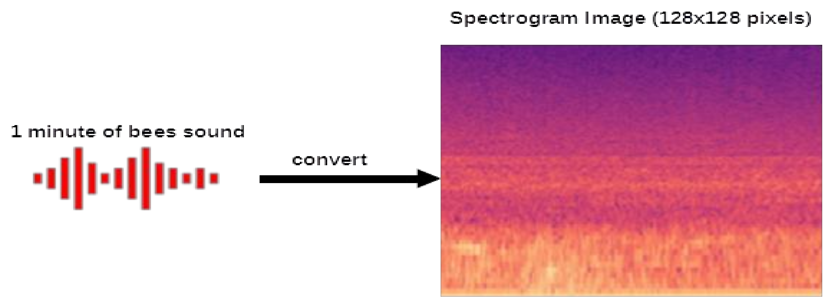
Only one-third of data are labeled Swarming because of the probability of a swarming event, which does not exceed 20%. Finally, the recording data from the experiment shows that one minute is long enough to illustrate the requested information by dividing the x-axis into 128-time points of 0.468 ms duration, as shown in
Figure 1.
For each single-minute sound described above, the corresponding Mel Spectrogram 128 × 128 px image is created, illustrating time points on the x-axis and frequency on the y-axis (center frequency of 128 equally-spaced Mel bands in the frequency spectrum of 0–10 kHz). The brightness of the pixels represents the per band aggregate sum RMS values expressed in dBmV values (on the logarithmic Voltage scale transformation, see
Appendix A).
Therefore, the data we used for the algorithm training consists of 23,760 Mel Spectrogram images that had either the Swarming or the Non-Swarming label. This set will be applied to the U-Net CNN algorithm for training and testing.
3.4. SVM and k-NN and U-Net Processing and Training Methods
Firstly, the SVM classifier was applied to the dataset with a polynomial kernel and penalty hyperparameter C = 1 (see
Appendix A, SVM parameters). The classifier was applied to the dataset, using 20% of it for testing (845 vectors) and the rest for training (3380 vectors). The kernel and parameters used arise from experimentation to find the optimal and most accurate result and are analytically explained in
Appendix A.
Next, using the same dataset, the k-NN classifier was trained. k-NN’s hyperparameters include the kernel and the number of k-neighbors. After fine-tuning (
Figure A2), the Euclidian kernel with k = 9 neighbors was selected. Twenty percent of the dataset was used for testing the classifier and the rest was used for training it. For the classifier evaluation experiments described in
Section 4, a different dataset was used, including a different proportion of annotated vectors of 33% swarming and 66% non-swarming data.
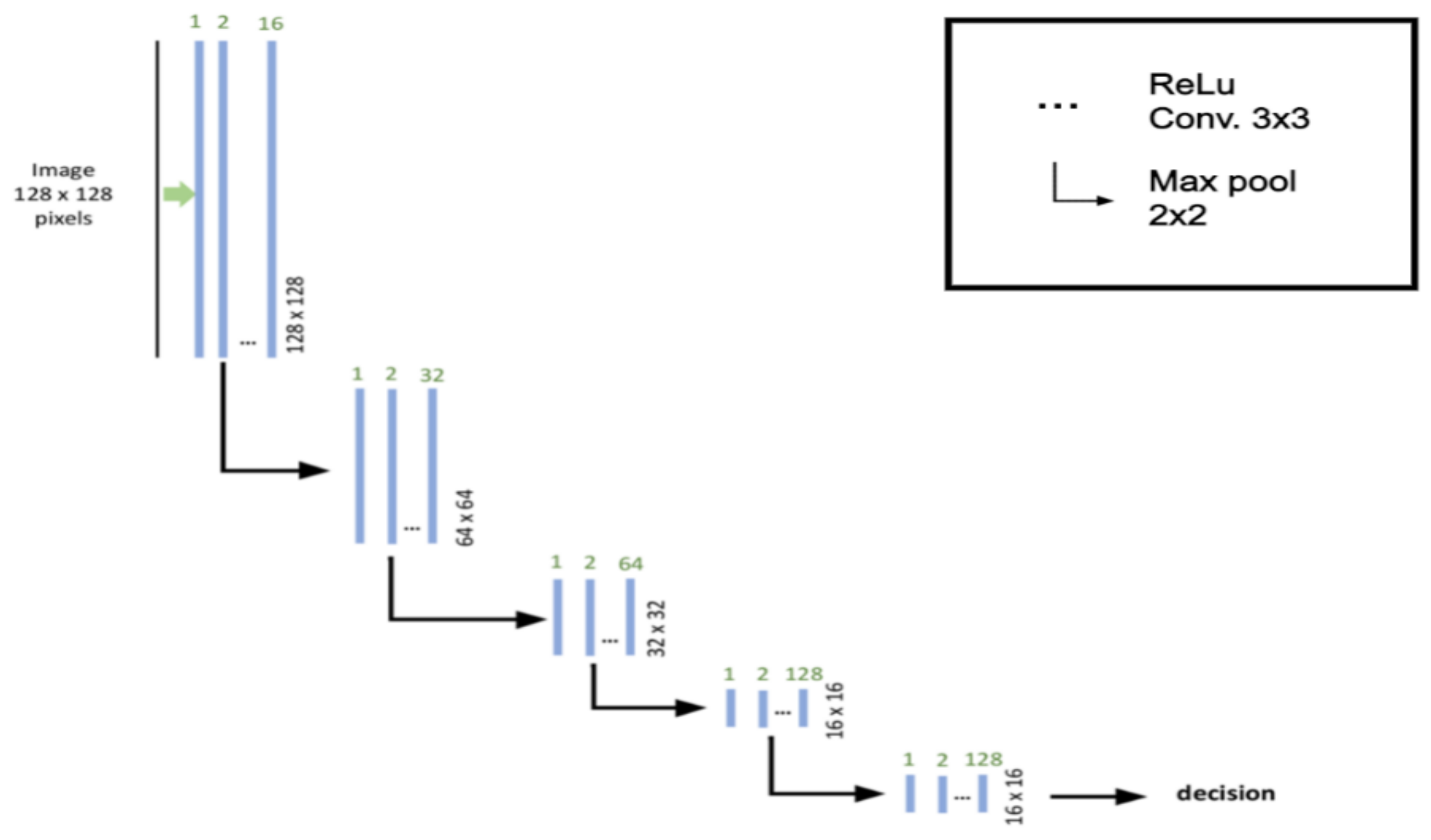
A novel Convolutional Neural Network (CNN) U-Net [
27] was also used (
Figure 2). The U-Net parameters used are the default parameters presented in
Appendix A.
Figure 2.
Analysis of the CNN U-Net used. Each blue box corresponds to a multi-channel feature map. The number of channels is denoted on top of the box. The x-y-size is provided at the lower left edge of the box [
22].
Figure 2.
Analysis of the CNN U-Net used. Each blue box corresponds to a multi-channel feature map. The number of channels is denoted on top of the box. The x-y-size is provided at the lower left edge of the box [
22].
The U-Net CNN training dataset used was the same as that used by the SVM and k-NN classifiers. The half U-Net model was used in order to simplify the segmentation process using five convolution layers, as illustrated in
Figure 2, along with the following parameters:
Activation function: Rectified Linear Unit (ReLU)
Epochs: 20
Input size: 128 × 128 pixels
Number of layers: 6 (5 convolutions + 1 decision)
The U-Net CNN training data imagery input includes swarming and non-swarming 1-min images (128 px on the x-axis of
Figure 3) and 128 bins on the y-axis expressed in the Mel scale, providing a better resolution at low frequencies. The logarithmic transformation of frequencies to Mels is given in
Appendix A.
4. k-NN, SVM, and U-Net CNN Algorithms Evaluation
This section includes the authors’ evaluation of the classification algorithms on their experimental scenario collection of swarming and non-swarming data. The evaluation efforts focus on the accurate early and close-to-the-event detection events, providing per-classifier and cross-comparison results.
4.1. Experimental Scenario
The authors’ evaluation scenario included five hives with a population capacity of 10 frames and a queen age range of 1 to 2 years (
Table 2). The IoT device was placed to record the sound produced by the beehives. In the location where the experiment took place, spring flowering had not yet begun. However, when flowering started in the area, the bee swarms started collecting pollen and nectar, resulting in daily exponential growth.
Sound recording for each swarm was performed twice every 24 h from the day the equipment was placed until the day of swarming. More specifically, for each day, a 12-h audio recording was carried out as follows:
All beehives (2–5) developed swarming events, with the first event beginning at the end of the spring bloom. After two swarming events, the beehive was replaced with another of similar characteristics under the same stressful conditions. This resulted in 4 out of 5 almost concurrent swarming events and a total of 12 swarming events for the whole season (2–3 per Beehive ID), as presented in
Table 3.
In order not to overlap the “fluttering” of the bees with the fact of their flight, due to usual everyday activity, only the sounds of their night activity were used in the sound analysis methods. Consequently, 6 h of audio was used from each beehive. Even though the day of swarming was unknown, the continual observation of the hives, with the assistance of professional apiarists, provided us with the appropriate feedback information.
The research presented in this paper took place in Ioannina, Greece, from March to July 2022 (five months). Therefore, the experiment was performed during the swarming season. The experiment site was located at the University of Ioannina beekeeping station located in the area of Ligopsa, Ioannina, Greece. Five beehive IoT monitoring devices have been implemented for this purpose. Moreover, the authors performed daily checks on the beehives’ conditions with a professional beekeeper’s assistance, indicating probable swarming events (formation of queen cells). The experiment site was 30 km from Ioannina city, where urban noises during the day could not add noise to the experiment altering the results.
The recorded data of 6 h were cropped into 360 single-minute audio files. Next, according to the apiarists’ observations, all audio files were annotated into swarming data up to 10 days before the swarming event. Additionally, all sounds up to 20 days before swarming were converted into non-swarming data. Finally, every single-minute audio file was classified into one of the above classes creating a total of 23,760 single-minute.wav audio files for the experimentation procedure.
Although the authors’ evaluation was performed using a limited number of IoT devices (five in total), with the help of the beekeepers, these five hives were selected and stressed to force swarming so the aims of the paper could be achieved. For every six hours of raw data recordings, 983 Mbytes of data are stored, almost 2 GB per hive per day. The evaluation experiments were performed in five beehives for five months capturing twelve swarming events and receiving a dataset for swarming events of 0.48 TBytes and 0.64 TBytes of non-swarming events.
4.2. Experimental Preprocessing Results
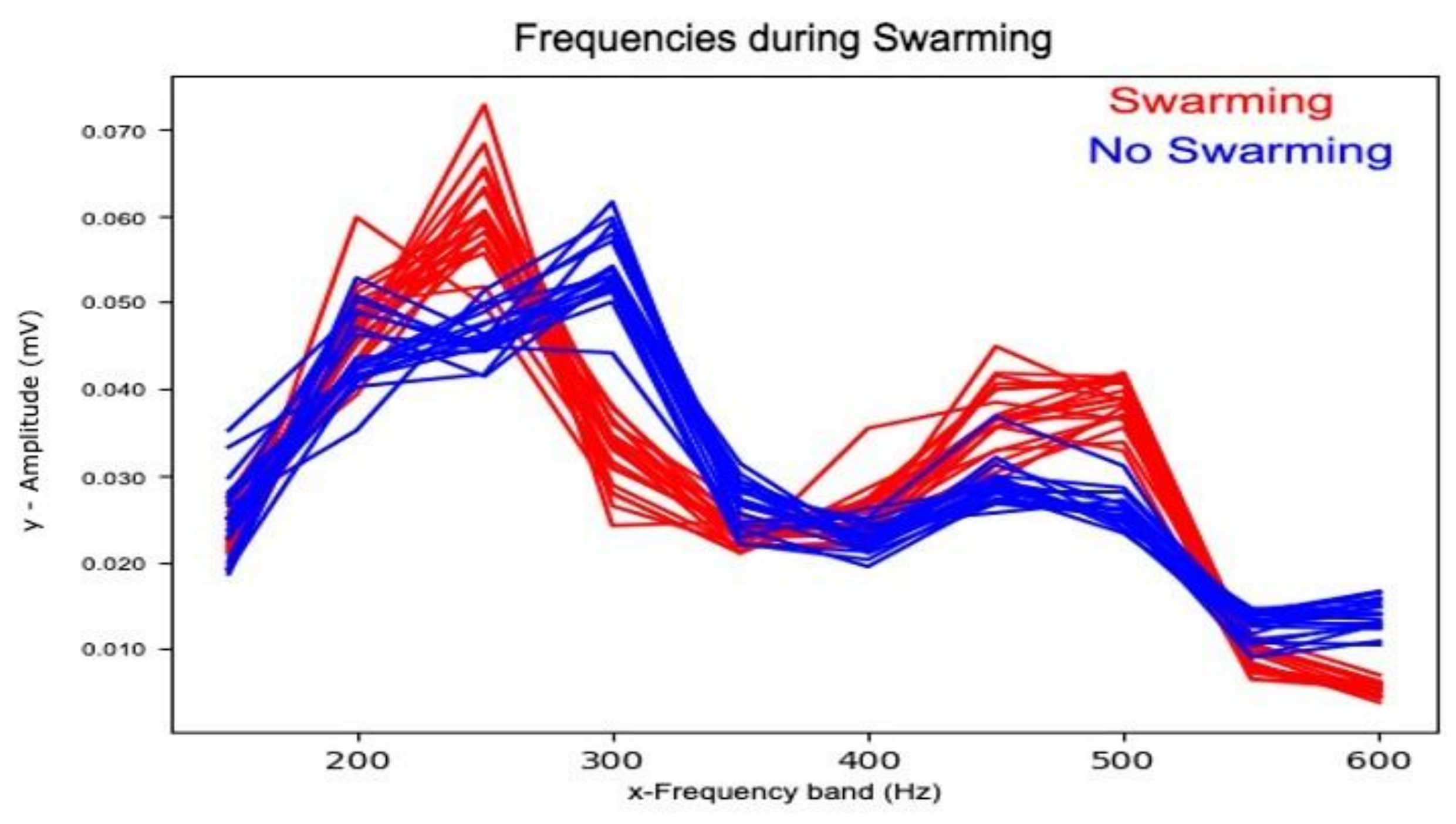
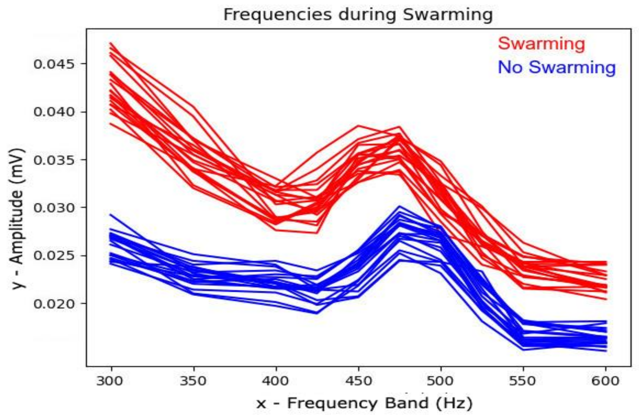
The main differences in bees’ behavior during swarming events are detected in the frequency range of 400–500 Hz. In addition, there are some minor noticeable differences in the frequency ranges of 200–300 Hz. The first part of our experiments was to prove that the critical range when swarming events are detected is, according to previous studies, 400–500 Hz.
Figure 4 shows the Fast Fourier Transformation results during swarming in the 150–600 Hz range. Experiments have shown that for such small differences, the classifiers cannot distinguish between swarming and non-swarming events, leading to wrong predictions and very low accuracy (below 70%). Therefore, the experimentation of SVM, k-NN classifiers, and training focuses only on the critical range of 300–600 Hz, where the swarming events can be easily recognized (see
Figure 5). Conversely, the U-Net CNN classifier uses the entire LPF-filtered spectrum as input.
As shown in
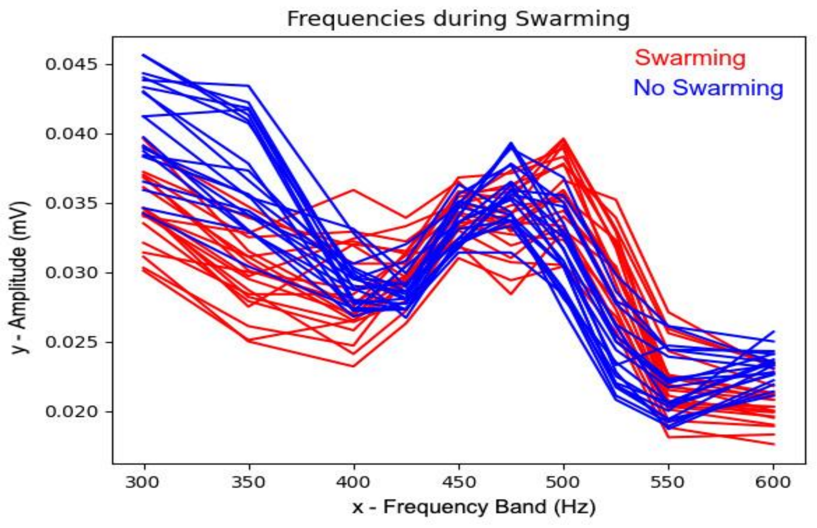
Figure 5, the frequencies of the bees’ sound during swarming events rapidly shift to 400–500 Hz, providing information to detect the event. Thus, to detect the swarming event early, we needed to examine the frequency’s changes ten days before swarming. The results are shown in
Figure 6 and explained below.
As is shown in
Figure 6, ten days before the swarming event, there are some noticeable differences in frequency bins between the two cases (swarming, non-swarming). However, there are many points where the two cases match. This affects the classifiers’ discrimination, reducing their accuracy.
4.3. SVM Classifier Results
This subsection presents the results of the SVM classifier with the polynomial kernel and C = 1, applied for five and ten days. In addition, the results contain the confusion matrix, Precision, Recall, F1-score, macro average, and weighted average. Definitions of those evaluators are given in
Appendix B.
As shown in the preprocessing phase, classifiers would provide a highly accurate result for swarming detection five days before the event. The confusion matrix of this experiment is shown in
Table 4, using the calibrated hyperparameters
As shown in
Table 5, SVM provides a high (97%) accuracy, while the precision of swarming reaches 98%. The results arose from 366 samples of swarming and 1024 samples of non-swarming raw sound data recordings.
The confusion matrix in
Table 6 is the result of the SVM ten days before the swarming event with the calibrated hyperparameters.
As expected, the results did not provide as high accuracy as the experiment applied in 5 days. Although, with 90% accuracy, it can be considered an accurate classifier to detect swarming events early. The results of this experiment are shown in
Table 7 and are taken from 350 samples of swarming and 966 non-swarming raw sound data recordings.
4.4. k-NN Classifier Results
The results of the k-NN are presented in this subsection, applied for 5 and 10 days, respectively, using the Euclidian distance kernel for k = 9 nearest neighbors (see
Appendix A, calibration of the k-NN parameters and
Figure A2). The confusion matrix in
Table 8 is the testing result of the k-NN, five days before the swarming event, with the calibrated hyperparameters.
As shown in
Table 9, k-NN provides 98% accuracy; thus, k-NN into the most accurate classifier for detecting swarming five days before the event. The results are presented in
Table 9 and were similarly taken in proportion to the SVM classifier from 249 samples and 837 samples of Non-swarming raw sound data recordings.
The confusion matrix in
Table 10 is the k-NN testing results ten days before the swarming event with the calibrated hyperparameters
Despite the close-to-the-event high detection accuracy that the k-NN classifier can provide, as shown in
Table 11, in the range of 10 days, k-NN scores a low 85% accuracy compared to the SVM classifier. The results of 10 days were similarly taken in proportion to the SVM classifier from 350 samples of swarming and 966 samples of Non-swarming raw sound data recordings.
4.5. U-Net Classifier Results
For the U-Net CNN classifier, the model’s accuracy was examined ten days before the swarming event. The results are presented in
Table 12, using the default network parameters mentioned in
Appendix A.
Focusing on early detection, the accuracy results of the U-Net classifier present an 89% mean accuracy. For late detection, a 92% mean accuracy is achieved for both swarming and non-swarming events. These are fairly-good accuracy results for both early and late detection cases.
Since the U-Net CNN utilizes the whole 10 kHz spectrum for its training and detection process, the results are an indication that it will outperform both k-NN and SVM if a more targeted data input is used; that is if the training applies in the frequency band of up to 1–2 kHz, followed by appropriate fine-tuning of its network parameters, such as the number of training steps.
4.6. Classifiers Comparative Study
The results of the three examined methods were presented in the previous subsections. In this subsection, using the common metric of accuracy, the results for these methods five and ten days before the swarming events are presented in
Table 13.
As shown in
Table 13, SVM has the highest accuracy (90%) for late swarming detection events, while k-NN fails to detect swarming events accurately, with an overall accuracy score of 85%. U-Net CNN is slightly outperformed by SVM, but outperforms k-NN, for late detection events, providing a score close to the SVM’s 89% accuracy score. U-Net CNN’s 89% accuracy for early detection seems to demonstrate great potential if appropriate data input filtering in the 0–2 kHz band is enforced in its training process. The authors set further experimentation with the U-Net CNN towards that direction as future work.
As shown in
Table 13, k-NN has the highest accuracy results (98%) for late swarming detection, closely followed by SVM with 97%. U-Net CNN follows with 95% accuracy, which is close to the SVM and k-NN classifier results.
Additionally, when it comes to using images (such as the ones used by the U-Net CNN) for the swarming detection process, the need for huge amounts of communication data can be avoided, reducing the energy expenditure of IoT devices. For example, periodic data uploads in raw sound form (2.69–3.5 Mbytes per minute snapshots), required by k-NN and SVM, need 10–20 times more than the U-Net CNN with the IoT device CPU set in an idle state. In contrast, fast processing and uploading of single image Mel spectrograms, as required by the U-Net CNN classifier, is much more device energy efficient. This problem can be alleviated for SVM and k-NN if part of the processing is performed at the IoT device, providing dimensionality reduction of discrete frequency vectors in a CSV file sent to the cloud.
5. Conclusions
This paper presents three different classification methods of processing the sound of bees inside a beehive before a swarming event in two distinct cases of detecting swarming events: late and early. The classifiers used for this purpose were the SVM, k-NN, and U-Net CNN. The authors present in detail their newly proposed U-Net classifier. Additionally, appropriate IoT devices have been constructed for collecting sound data and classifiers’ experimental evaluation.
After the authors’ preliminary experiments on recorded sound data and verification of the frequency band that significant deviations occur during swarming events, as well as calibration of the classifiers’ parameters and training, evaluation of the classifiers followed.
The results show that k-NN and SVM, which are already used for bee sound analysis processes, provide the most accurate results for late and early detection of swarming, respectively. Focusing on early detection, which can alleviate or prevent the event, our experiment showed that SVM is the most appropriate method, while k-NN fails to detect it accurately. For early detecting swarming events, U-Net CNN performs almost as equally well as SVM and has the potential to perform even better with frequency-targeted data input and model parameters fine-tuning. The authors set, as future work, the extensive evaluation of the proposed U-Net CNN algorithm fine-tuning towards swarming events and the extension of their experiments to other deep learning algorithms.
Author Contributions
Conceptualization, K.I.D., S.K., G.S.S., C.V.B. and K.A.S.; Funding acquisition, C.V.B., K.A.S. and G.S.S.; Investigation, K.I.D.; Methodology, G.S.S. and S.K.; Resources, C.V.B., K.A.S. and G.S.S.; Software, K.I.D., T.K. and I.A.; Supervision, S.K.; Writing—original draft, K.I.D. and I.A.; Writing—review & editing, C.V.B. and S.K. All authors have read and agreed to the published version of the manuscript.
Funding
This research has been funded by the Lime Technology company and the European Union and Greek national funds through the Operational Program Competitiveness, Entrepreneurship and Innovation, under the call RESEARCH–CREATE–INNOVATE (project code: T2EDK-2402).
Data Availability Statement
Not applicable.
Acknowledgments
This research has been co-financed by the European Union and Greek national funds through the Operational Program Competitiveness, Entrepreneurship and Innovation, under the call RESEARCH–CREATE–INNOVATE (project code: T2EDK-2402).
Conflicts of Interest
The authors declare no conflict of interest.
Appendix A. Classification Algorithms Optimization
Parameters optimization to achieve the best accurate results using k-NN and SVM has been conducted by experimenting with the possible combinations of parameters. The results of parameters fine-tuning for SVM and k-NN classifiers are shown in
Figure A1 and
Figure A2 and explained below.
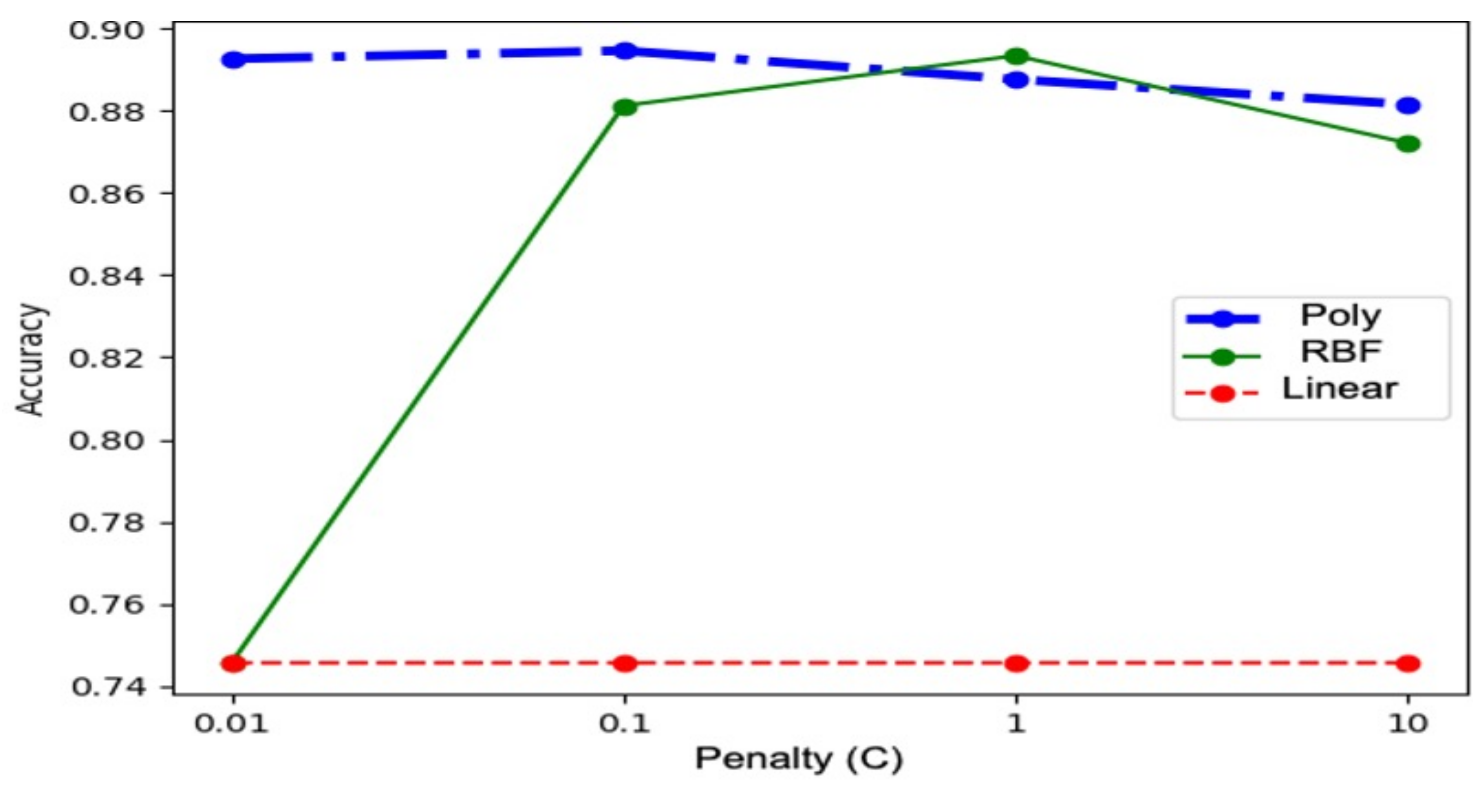
The SVM classifier includes two major hyperparameters: the kernel and the penalty (C) value, as shown in
Figure A1. The most common kernels for SVM are the examined linear, polynomial, and Radial Basis Function (RBF) kernels. Of these three, RBF and polynomial provided the most accurate results, with the polynomial performing slightly better for a range of penalty values C [0.01–10]. The penalty C metric can take a range of values that may exponentially affect classification accuracy. Therefore, log scales are usually preferred on this parameter, and the chosen values of C are 0.01, 0.1, 1, and 10. Therefore, penalty values below 0.01 or above 10 have not been examined. As shown in
Figure A1, for C = 1 the SVM classifier accuracy peaks for either polynomial or RBF kernels. Nevertheless, the polynomial kernel has been selected due to its better accuracy response for C values below 1.
Figure A1.
Accuracy of different SVM classifier kernels over the values of penalty C values.
Figure A1.
Accuracy of different SVM classifier kernels over the values of penalty C values.
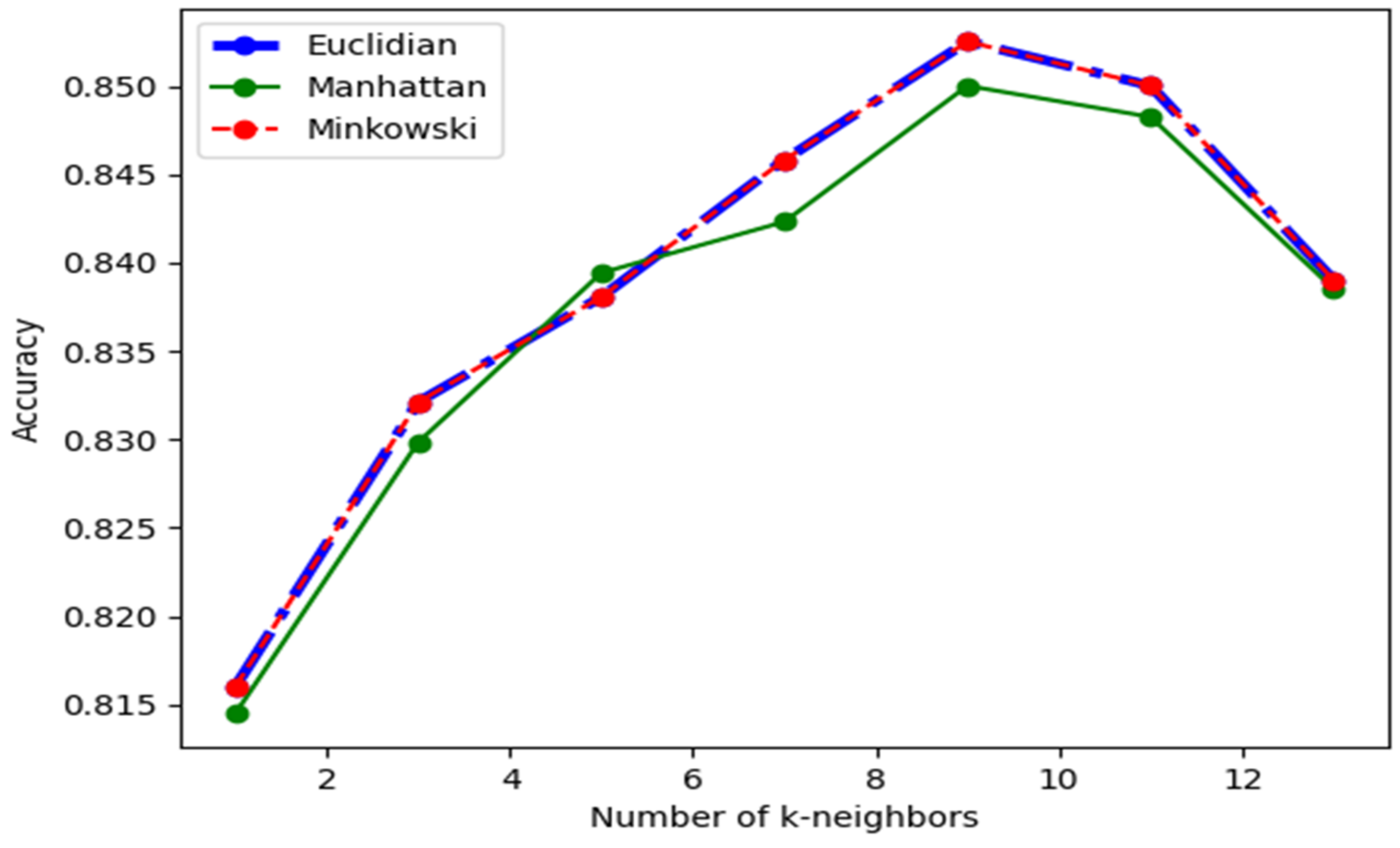
The k-NN classifier includes two parameters: the number of neighbors (
n) and the distance metric used. The number of neighbors is the most important hyperparameter of k-NN, and it usually takes odd values in the range of 1–21. Experiments showed that the accuracy follows a decreasing curve for
n > 9 for our training dataset and for k-value
n = 9, which is a local maximum point and, therefore, the optimal parameter choice. For distance metrics, Euclidian and Minkowski’s metrics presented similar accuracy results over the number n of k-values. Parameters calibration experiments showed that for both uniform and distance weightings, the contribution of neighborhood members had minimal impact, which is why they are not included in
Figure A2.
Figure A2.
Accuracy of different distance measures over the number (n) of k-neighbors used for the k-NN classifier.
Figure A2.
Accuracy of different distance measures over the number (n) of k-neighbors used for the k-NN classifier.
Finally, for the CNN U-Net 6-layer model (half U-Net model), the training epochs have been fine-tuned to 20 epochs, minimizing total loss to 0.08. T. Equation A1 provides the mapping between frequencies and Mels.
A1. Frequency (f) to Mel (m) transformation is defined as: .
A2. Voltage dB (dBmV) transformation from mV RMS is defined as: .
Appendix B. Evaluation Metrics Used
B1. Precision in binary classification is defined as: .
B2. Recall in binary classification is defined as: .
B3. F1-score in binary classification is defined as: .
B4. Accuracy in binary classification is defined as: .
B5. The macro average is calculated using the arithmetic mean as: , where is the class value and n is the number of classes.
B6. The weighted average is calculated by taking the mean of all per-class values while considering the support of each class (actual occurrences of the class), defined as: , where the class value, is the ratio of the total class instances over all instances (support), and n is the number of classes.
References
- Talavera, J.M.; Tobon, L.E.; Gómez, J.A.; Culman, M.A.; Aranda, J.M.; Parra, D.T.; Quiroz, L.A.; Hoyos, A.; Garreta, L.E. Review of IoT applications in agro-industrial and environmental fields. Comput. Electron. Agric. 2017, 142, 283–297. [Google Scholar] [CrossRef]
- Mpikos, A.T. What I Have to Do in My Beehives—The Real Beekeeping; Protoporia: Athens, Greece, 2010; ISBN 9789609931601. (In Greek) [Google Scholar]
- Stabentheiner, A.; Kovac, H.; Brodschneider, R. Honeybee Colony Thermoregulation—Regulatory Mechanisms and Contribution of Individuals in Dependence on Age, Location and Thermal Stress. PLoS ONE 2010, 5, e8967. [Google Scholar] [CrossRef] [PubMed]
- Karakousis, D. Apiarist’s Experiences; Stamoulis Publications: Athens, Greece, 2013; ISBN 9789603519454. (In Greek) [Google Scholar]
- Terenzi, A.; Ortolani, N.; Nolasco, I.; Benetos, E.; Cecchi, S. Comparison of Feature Extraction Methods for Sound-Based Classification of Honey Bee Activity. IEEE ACM Trans. Audio Speech Lang. Process. 2021, 30, 112–122. [Google Scholar] [CrossRef]
- Mekha, P.; Teeyasuksaet, N.; Sompowloy, T.; Osathanunkul, K. Honey Bee Sound Classification Using Spectrogram Image Features. In Proceedings of the 2022 Joint International Conference on Digital Arts, Media and Technology with ECTI Northern Section Conference on Electrical, Electronics, Computer and Telecommunications Engineering (ECTI DAMT & NCON), Chiang Rai, Thailand, 26–28 January 2022; pp. 205–209. [Google Scholar] [CrossRef]
- Winston, M.L. Intra-colony demography and reproductive rate of the Africanized honeybee in South America. Behav. Ecol. Sociobiol. 1979, 4, 279–292. [Google Scholar] [CrossRef]
- Seeley, T.D.; Tautz, J. Worker piping in honey bee swarms and its role in preparing for liftoff. J. Comp. Physiol. A Sens. Neural Behav. Physiol. 2001, 187, 667–676. [Google Scholar] [CrossRef] [PubMed]
- Robles-Guerrero, A.; Saucedo-Anaya, T.; Ramirez, E.G.; Tejada, C.J. Frequency analysis of honey bee buzz for automatic recognition of health status: A preliminary study. In Proceedings of the International Conference on Computer Networks Applications (ICCNA), Mexicali, Mexico, 6–8 November 2018; pp. 89–98. [Google Scholar]
- Abou-Shaara, H.F.; Owayss, A.A.; Ibrahim, Y.Y.; Basuny, N.K. A review of impacts of temperature and relative humidity on various activities of honey bees. Insectes Soc. 2017, 64, 455–463. [Google Scholar] [CrossRef]
- Nolasco, I.; Terenzi, A.; Cecchi, S.; Orcioni, S.; Bear, H.L.; Benetos, E. Audio-based identification of beehive states. In Proceedings of the CASSP 2019—2019 IEEE International Conference on Acoustics, Speech and Signal Processing (ICASSP), Brighton, UK, 12–17 May 2019; pp. 8256–8260. [Google Scholar] [CrossRef]
- Nolasco, I.; Benetos, E. To Bee or Not to Bee: Investigating machine learning approaches for beehive sound recognition. In Proceedings of the Detection and Classification of Acoustic Scenes and Events 2018 Workshop (DCASE2018), Surrey, UK, 19–20 November 2018. [Google Scholar] [CrossRef]
- Terenzi, A.; Cecchi, S.; Orcioni, S.; Piazza, F. Features Extraction Applied to the Analysis of the Sounds Emitted by Honey Bees in a Beehive. In Proceedings of the 2019 11th International Symposium on Image and Signal Processing and Analysis (ISPA), Dubrovnik, Croatia, 23–25 September 2019; pp. 3–8. [Google Scholar] [CrossRef]
- Ferrari, S.; Silva, M.; Guarino, M.; Berckmans, D. Monitoring of swarming sounds in bee hives for early detection of the swarming period. Comput. Electron. Agric. 2008, 64, 72–77. [Google Scholar] [CrossRef]
- Ramsey, M.-T.; Bencsik, M.; Newton, M.I.; Reyes, M.; Pioz, M.; Crauser, D.; Delso, N.S.; Le Conte, Y. The prediction of swarming in honeybee colonies using vibrational spectra. Sci. Rep. 2020, 10, 9798. [Google Scholar] [CrossRef] [PubMed]
- Howard, D.; Duran, O.; Hunter, G. A low-cost multi-modal sensor network for the monitoring of honeybee colonies/hives. In Intelligent Environments 2018; Ambient Intelligence and Smart Environments; IOS Press BV: Amsterdam, The Netherlands, 2018; Volume 23, pp. 69–78. [Google Scholar] [CrossRef]
- Bencsik, M.; Bencsik, J.; Baxter, M.; Lucian, A.; Romieu, J.; Millet, M. Identification of the honey bee swarming process by analysing the time course of hive vibrations. Comput. Electron. Agric. 2011, 76, 44–50. [Google Scholar] [CrossRef]
- Hunter, G.; Howard, D.; Gauvreau, S.; Duran, O.; Busquets, R. Processing of multi-modal environmental signals recorded from a “smart” beehive. Proc. Inst. Acoust. 2019, 41, 339–348. [Google Scholar]
- Gil-Lebrero, S.; Quiles-Latorre, F.J.; Ortiz-López, M.; Sánchez-Ruiz, V.; Gámiz-López, V.; Luna-Rodríguez, J.J. Honey Bee Colonies Remote Monitoring System. Sensors 2016, 17, 55. [Google Scholar] [CrossRef] [PubMed]
- Nieh, J.; Tautz, J. Behaviour-locked signal analysis reveals weak 200–300 Hz comb vibrations during the honeybee waggle dance. J. Exp. Biol. 2000, 203, 1573–1579. [Google Scholar] [CrossRef] [PubMed]
- Zacepins, A.; Kviesis, A.; Ahrendt, P.; Richter, U.; Tekin, S.; Durgun, M. Beekeeping in the future—Smart apiary management. In Proceedings of the 2016 17th International Carpathian Control Conference (ICCC), High Tatras, Slovakia, 29 May–1 June 2016; pp. 808–812. [Google Scholar] [CrossRef]
- Zacepins, A.; Kviesis, A.; Pecka, A.; Osadcuks, V. Development of internet of things concept for precision beekeeping. In Proceedings of the 2017 18th International Carpathian Control Conference (ICCC), Sinaia, Romania, 28–31 May 2017; Volume 1, pp. 23–27. [Google Scholar] [CrossRef]
- Bellos, C.V.; Fyraridis, A.; Stergios, G.S.; Stefanou, K.A.; Kontogiannis, S. A Quality and disease control system for beekeeping. In Proceedings of the 2021 6th South-East Europe Design Automation, Computer Engineering, Computer Networks and Social Media Conference (SEEDA-CECNSM), Preveza, Greece, 24–26 September 2021; pp. 1–4. [Google Scholar] [CrossRef]
- Zgank, A. Bee Swarm Activity Acoustic Classification for an IoT-Based Farm Service. Sensors 2019, 20, 21. [Google Scholar] [CrossRef] [PubMed]
- Zgank, A. Acoustic monitoring and classification of bee swarm activity using MFCC feature extraction and HMM acoustic modeling. In Proceedings of the ELEKTRO 2018, Mikulov, Czech Republic, 21–23 May 2018; pp. 1–4. [Google Scholar] [CrossRef]
- Voudiotis, G.; Kontogiannis, S.; Pikridas, C. Proposed Smart Monitoring System for the Detection of Bee Swarming. Inventions 2021, 6, 87. [Google Scholar] [CrossRef]
- Ronneberger, O.; Fischer, P.; Brox, T. U-Net: Convolutional networks for biomedical image segmentation. In Medical Image Computing and Computer-Assisted Intervention 2015; Navab, N., Hornegger, J., Wells, W.M., Frangi, A.F., Eds.; Springer International Publishing: Cham, Switzerland, 2015; Volume 9315, pp. 234–241. [Google Scholar] [CrossRef]
Figure 1.
Conversion of bee raw sound data to 128-bin Mel spectrogram Image.
Figure 1.
Conversion of bee raw sound data to 128-bin Mel spectrogram Image.
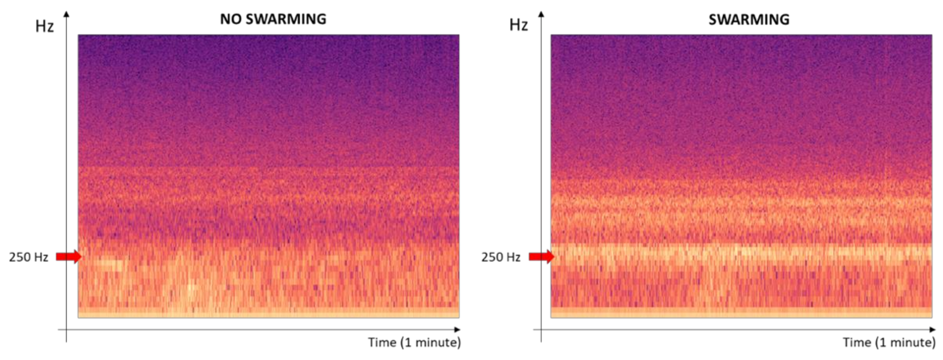
Figure 3.
Swarming and non Swarming Mel spectrograms. The left image is during a non-swarming event, and the right image is five days before a swarming event.
Figure 3.
Swarming and non Swarming Mel spectrograms. The left image is during a non-swarming event, and the right image is five days before a swarming event.
Figure 4.
Frequencies 5 days before a swarming event in the frequency band of 150–600 Hz.
Figure 4.
Frequencies 5 days before a swarming event in the frequency band of 150–600 Hz.
Figure 5.
Amplitude response in mV RMS, 5 days before the swarming event over the frequency band of 300–600 Hz (using 10/25 Hz frequency bins).
Figure 5.
Amplitude response in mV RMS, 5 days before the swarming event over the frequency band of 300–600 Hz (using 10/25 Hz frequency bins).
Figure 6.
Amplitude response in mV RMS ten days before the swarming event over the frequency band of 300–600 Hz (using 10/25 Hz frequency bins).
Figure 6.
Amplitude response in mV RMS ten days before the swarming event over the frequency band of 300–600 Hz (using 10/25 Hz frequency bins).
Table 2.
Age of the queen bee in different hives of the experiment.
Table 2.
Age of the queen bee in different hives of the experiment.
| Bee Colony Hive ID | Age of Queen Bee |
|---|
| 1 | 1 year old/non-stressed |
| 2 | 2 years old/stressed * |
| 3 | 2 years old/stressed * |
| 4 | 2 years old/stressed * |
| 5 | 2 years old/stressed * |
Table 3.
Swarming date in the different hives of the experiments.
Table 3.
Swarming date in the different hives of the experiments.
| Bee Colony Hive ID | First Swarming Date | Number of Swarming Events |
|---|
| 1 | Non-Swarming | 0 |
| 2 | 8 May 2022 | 4 |
| 3 | 24 May 2022 | 2 |
| 4 | 13 May 2022 | 3 |
| 5 | 17 May 2022 | 3 |
Table 4.
Confusion matrix of SVM classifier applied five days before the swarming event.
Table 4.
Confusion matrix of SVM classifier applied five days before the swarming event.
| | True | False |
|---|
| Positive | 354 | 12 |
| Negative | 16 | 1008 |
Table 5.
SVM Classifier results applied five days before the swarming event.
Table 5.
SVM Classifier results applied five days before the swarming event.
| | Precision | Recall | F1-Score | Accuracy |
|---|
| 0.0 (Non-Swarming) | 96% | 95% | 96% | - |
| 1.0 (Swarming) | 98% | 98% | 98% | - |
| Accuracy | - | - | - | 97% |
| Macro avg | 97% | 97% | 97% | - |
| Weighted avg | 97% | 97% | 97% | - |
Table 6.
Confusion matrix of SVM classifier applied ten days before the swarming event.
Table 6.
Confusion matrix of SVM classifier applied ten days before the swarming event.
| | True | False |
|---|
| Positive | 306 | 44 |
| Negative | 82 | 884 |
Table 7.
SVM Classifier results applied ten days before the swarming event.
Table 7.
SVM Classifier results applied ten days before the swarming event.
| | Precision | Recall | F1-Score | Accuracy |
|---|
| 0.0 (Non-Swarming) | 79% | 87% | 83% | - |
| 1.0 (Swarming) | 95% | 92% | 93% | - |
| Accuracy | - | - | - | 90% |
| Macro avg | 87% | 89% | 88% | - |
| Weighted avg | 91% | 90% | 91% | - |
Table 8.
Confusion matrix of k-NN classifier applied five days before the swarming event.
Table 8.
Confusion matrix of k-NN classifier applied five days before the swarming event.
| | True | False |
|---|
| Positive | 245 | 4 |
| Negative | 25 | 812 |
Table 9.
k-NN Classifier results applied 5 days before the swarming event.
Table 9.
k-NN Classifier results applied 5 days before the swarming event.
| | Precision | Recall | F1-Score | Accuracy |
|---|
| 0.0 (Non-Swarming) | 99% | 98% | 99% | - |
| 1.0 (Swarming) | 98% | 98% | 98% | - |
| Accuracy | - | - | - | 98% |
| Macro avg | 98% | 98% | 98% | - |
| Weighted avg | 98% | 98% | 98% | - |
Table 10.
Confusion matrix of k-NN classifier applied 10 days before the swarming event.
Table 10.
Confusion matrix of k-NN classifier applied 10 days before the swarming event.
| | True | False |
|---|
| Positive | 246 | 104 |
| Negative | 84 | 882 |
Table 11.
k-NN Classifier results applied ten days before the swarming event.
Table 11.
k-NN Classifier results applied ten days before the swarming event.
| Precision | Recall | F1-Score | Accuracy |
|---|
| 0.0 (Non-Swarming) | 74% | 70% | 72% | - |
| 1.0 (Swarming) | 70% | 91% | 90% | - |
| Accuracy | - | - | - | 85% |
| Macro avg | 81% | 80% | 81% | - |
| Weighted avg | 85% | 86% | 85% | - |
Table 12.
Results of the U-Net CNN classifier.
Table 12.
Results of the U-Net CNN classifier.
| Days before the Swarming Event | Swarming Probability
(Recall) | Non-Swarming
Probability
(Recall) | Accuracy |
|---|
| 1–3 | 94% | 96% | 95% |
| 4–6 | 91% | 93% | 92% |
| 7–8 | 89% | 90% | 90% |
| 9–10 | 88% | 90% | 89% |
Table 13.
Cross-comparison results of all three methods.
Table 13.
Cross-comparison results of all three methods.
| Accuracy | SVM | k-NN | CNN |
|---|
Early detection
(10 days before swarming) | 90% | 85% | 89% |
Late detection
(5 days before swarming) | 97% | 98% | 95% |
| Publisher’s Note: MDPI stays neutral with regard to jurisdictional claims in published maps and institutional affiliations. |
© 2022 by the authors. Licensee MDPI, Basel, Switzerland. This article is an open access article distributed under the terms and conditions of the Creative Commons Attribution (CC BY) license (https://creativecommons.org/licenses/by/4.0/).


 ,
, 


