
Compressive Sensing Based Space Flight Instrument Constellation for Measuring Gravitational Microlensing Parallax


1
NASA Goddard Space Flight Center, Greenbelt, MD 20771, USA
2
Computer Science and Electrical Engineering Department, University of Maryland, Baltimore County, Baltimore, MD 21250, USA
*
Author to whom correspondence should be addressed.
Signals 2022, 3(3), 559-576; https://doi.org/10.3390/signals3030034
Submission received: 1 April 2022
/
Revised: 7 June 2022
/
Accepted: 28 June 2022
/
Published: 15 August 2022
(This article belongs to the Special Issue Compressive Sensing and Its Applications)
Abstract
:In this work, we provide a compressive sensing architecture for implementing on a space based observatory for detecting transient photometric parallax caused by gravitational microlensing events. Compressive sensing (CS) is a simultaneous data acquisition and compression technique, which can greatly reduce on-board resources required for space flight data storage and ground transmission. We simulate microlensing parallax observations using a space observatory constellation, based on CS detectors. Our results show that average CS error is less than using Nyquist rate samples. The error at peak magnification time is significantly lower than the error for distinguishing any two microlensing parallax curves at their peak magnification. Thus, CS is an enabling technology for detecting microlensing parallax, without causing any loss in detection accuracy.
1. Introduction
Gravitational microlensing is an astronomical phenomena. When a lensing body comes in precise alignment with a source star, which is being observed through an optical system, the light rays bend due to the gravitational effects of the lensing system, causing a magnification in the observed light curve. By obtaining these photometric curves and analyzing their characteristics, we can determine the science parameters of a lensing system. We show a compressive sensing (CS) based architecture system for a space flight constellation here, performing photometric measurements. Typically, the galactic bulge is surveyed in order to increase the chances of capturing a microlensing event. A space based microlensing parallax can be obtained using a CS architecture. A CS system will enable capturing and collecting data in SmallSat type instruments by reducing the need for on-board data storage and data downlink bandwidth.
Compressive sensing is a mathematical theory for sampling at a rate much lower than the Nyquist rate, and yet reconstructing the signal back with little or no loss of information. The signal is reconstructed by solving an underdetermined system. In a CS architecture, to acquire a signal of size n, we collect m measurements, where . One measurement sample consists of a collective sum. We solve for Equation (1) to determine x through the observation y [1,2,3,4].
Using the acquired measurements vector y and the known measurement matrix A, we can solve for a sparse x by applying various techniques, including greedy algorithms and optimization algorithms.
1.1. Motivation
We target our research for space flight instrumentation. For gravitational microlensing measurements, obtaining microlensing parallax is of critical importance in order to acquire properties of the lensing system. Our research enables development of a space flight instrument telescope constellation to acquire microlensing parallax measurements. These measurements would not be feasible on any SmallSat type instruments in a telescope constellation due to limited on-board resources available on these instruments—unless an intelligent and efficient way of sampling and compressing data is available, such as the one we demonstrate here using compressive sensing techniques.
1.2. Goals
The goal of this paper is to demonstrate the application of CS to acquire gravitational microlensing measurements. We aim to show that CS does not cause any significant errors in detection of gravitational microlensing parallax measurements through our theory-based simulation models.
1.3. Organization
This paper is organized in the following manner:
- In Section 2, we provide background on the theory of gravitational microlensing parallax measurements.
- In Section 3, we provide background on CS theory and its application for gravitational microlensing measurements.
- In Section 4, we show a potential CS detector implementation architecture for a telescope constellation.
- In Section 5, we describe our simulation and modelling setup.
- In Section 6, we provide our simulation results and analysis.
- In Section 7, we discuss data volume and on-board resources required for space instrument implementation.
- Finally, in Section 8, we provide conclusions.
2. Microlensing Parallax
In gravitational lensing, the surface brightness, which is the flux per area, is conserved. The total flux increases or decreases, since the area increases or decreases. In microlensing, distinct images, due to the gravitational effects of the lensing system, are not seen, but, instead, magnification or demagnification of the source star is observed; the images are not resolved. Since the Jacobian matrix gives the amount of change in the source star flux in each direction, the transformation of the original source to the stretched source can be mapped by the Jacobian. The absolute value of the inverse of determinant gives the amount of magnification.
Einstein’s ring forms when there is an exact alignment of the source, lens and observer and is an important parameter for the basis of gravitational microlensing equations. Einstein’s ring radius, , can be defined by Equation (2).
where M is the total mass of the lensing system, is the distance from the lens to the source, is the distance from the observer to the lensing system, and is the distance from the observer to the source [5].
From the formalization from [6], rewriting this in terms of relative lens-source parallax, , where , we obtain
Here and AU is 1 Astronomical unit or km.
The amplification of a single lensed microlensing event light curve with time dependency is given by Equation (6) [5].
Thus, from a photometric curve, for a single microlensing event, we can obtain the parameters: , , , and from a microlensing photometric curve. All of the parameters are defined in Table 1.
In Table 1, is the relative lens-source proper motion. Here, obtaining the lens mass remains unresolved, as we have two unknown parameters: and . In order to break the degeneracy to obtain specific microlensing parameters, measuring the parallax, , offers once such solution [9,10]. If we obtain , we can solve for M, given . According to [8], microlensing parallax can be measured in three ways:
- Motion of the Earth around the sun causing an annual parallax;
- Two or more space based observatories, separated by a significant baseline;
- Terrestrial parallax measured using a ground and space based observatory.
In our work, we focus on a constellation of a space based observatory to create simultaneous parallax measurements.
We can define the parallel and perpendicular shifts due to a microlensing parallax as in [6,8]. Let us assume as the vector for the motion of the observatory. In a telescope constellation, from [8], o = , where:
and
Here, and we use in our simulations.
The parallax vector , where is the lens source trajectory angle.
To obtain the shifts due to parallax, we obtain:
where , P is the orbital period, and is the orbital phase relative to [8]. We use in our modelling. From Equation (6), we can write
where .
We can define as the microlensing equations due to parallax [8]:
In this manner, we can define the new amplification equation as
Thus, from a photometric curve with a microlens parallax, we can obtain and .
3. CS Application for Gravitational Microlensing
3.1. CS Theory
Compressive sensing is a mathematical theory for sampling at a rate much lower than the Nyquist rate, and yet reconstructing the signal back with little or no loss of information. The signal is reconstructed by solving an underdetermined system. Sparsity in data sets is a key component required for the accuracy in reconstruction using CS methods. If it is not sparse in the sampling domain, we can transform it to a sparse domain, perform the reconstruction, and then transform it back to the original domain [3,4]. In a CS architecture, to acquire a signal of size n, we collect m measurements, where . One measurement sample consists of a collective sum. We solve for Equation (1) to determine x through the observation y [1,2,3,4]: We can then reconstruct x using the acquired measurements vector, y, and the known measurement matrtix, A.
3.2. CS Application
Transient events such as gravitational microlensing events can be detected using differenced imaging. In differenced imaging, we take a difference of a good seeing reference image with an observed image. We show a CS architecture for microlensing events, to obtain the differenced images, which contain the source star magnification flux as shown in Figure 1.
In architecture (Figure 1), differencing is applied to the CS measurements, resulting in a reconstructed differenced image. A photometric curve can then be generated using the flux of the source star pixels of the differenced image over time.
The architecture is implemented in the following manner:
- 1
- Obtain CS based measurements, , for a spatial image.CS can be applied by projecting a matrix, A, onto the region of interest, . This can be done on a column-by-column basis for a n × n spatial region, . Thus, for 2D images, and A are of size m × n, where .
- 2
- Given A and a clean reference image, , construct measurements matrix , where .
- 3
- Apply a 2D differencing algorithm on and to obtain a differenced image, , and the corresponding convolution kernel, M, which is used to match the observed and reference CS measurement vectors, and [11]. In our modelling, we use , by using the assumption that the PSF of the reference and observed image is the same. This assumption is valid for space flight instruments when both observed and reference images are obtained on-board the instrument.
- 4
- Reconstruct the differenced image, using CS reconstruction algorithms, given A and .
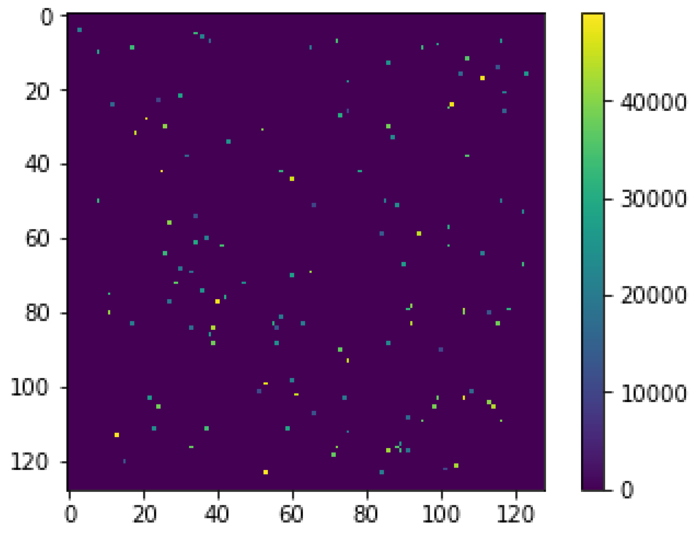
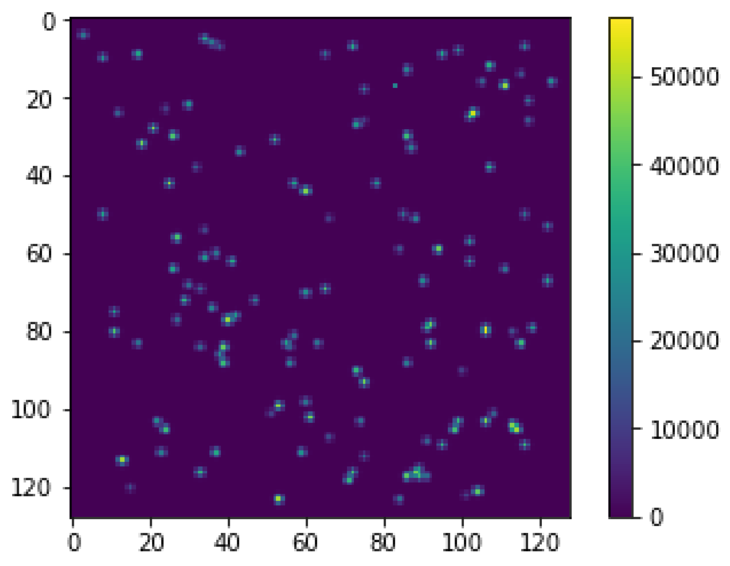
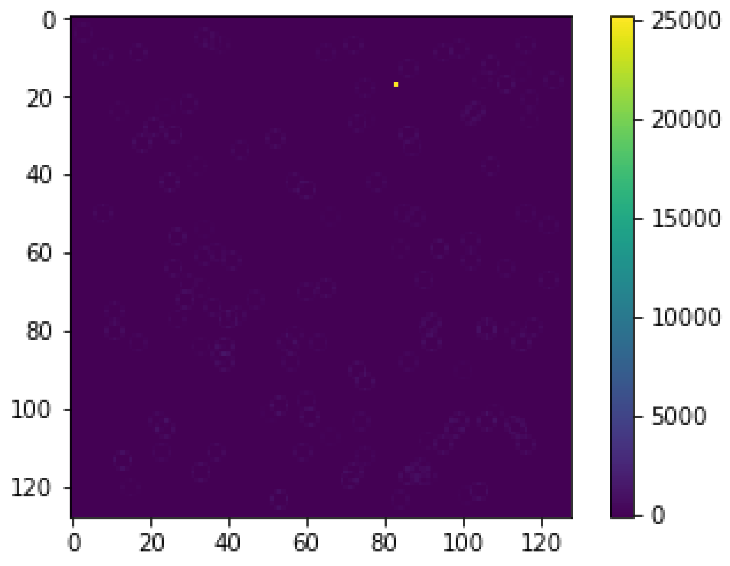
In our modelling, we assume the same PSF for the reference and observed image; hence, in an ideal scenario, we would obtain a differenced image with only the microlensing event present. A sample reference image, the observed image, a differenced image, is shown in Figure 2, Figure 3, and Figure 4, respectively.
CS reconstruction, using the architecture in Figure 1, reconstructs the differenced image.
4. CS Detector Architecture
There are numerous options for implementing a CS based detector system as discussed in [12,13,14]. Spatial light modulators are used to implement measurement matrices. Previous work by [15] show a CS implementation using coded aperture masks. In the literature from [16,17,18], they implemented a single pixel camera using liquid crystal displays (LCD). Their work shows that lensless single pixel cameras can be implemented using LCD as their coded apertures.
In our analysis, we focus on using a DMD array for the CS projection. A CS architecture using a DMD array can have a frame rate of 32 KHz with 2048 × 1080 pixels [13]. In our simulations, we show the effectiveness with 25% of n. Let us assume pixels. We would need 550,800 measurements. With the frame rate, this gives us 17.2 s to obtain one CS image, in addition to the needed exposure time. A typical microlensing event can last for 30 days. In [19], they discovered the shortest time scale microlensing event measured, where ≈ 41.5 min. Using Nyquist rate for this short time scale, we would expect to sample at least ≈ 20.75 s. Detection efficiency will not only depend on the cadence of the system but also on the flux magnification and Field-of-view (FOV). The larger the FOV, the greater the chances of detection of a microlensing event.
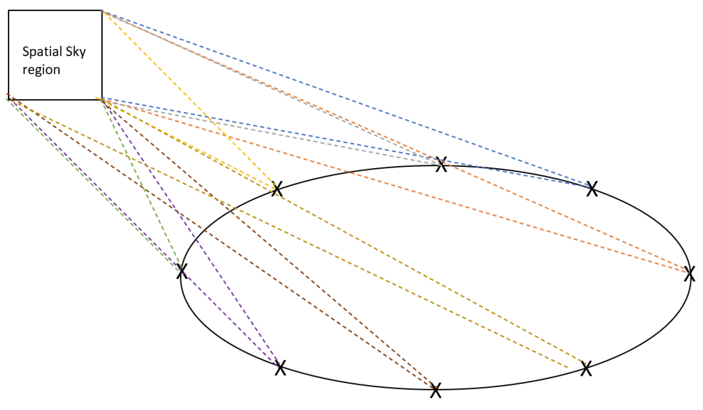
A CS detector system would be beneficial for use on Small Satellites, where data storage and downlink can be limiting factors. Using a CS detector system on a constellation of satellites, we can detect a microlensing parallax, as shown in Figure 5. In our simulations, we assume the number of satellites in the constellation to be [0, ], where the maximum number is .
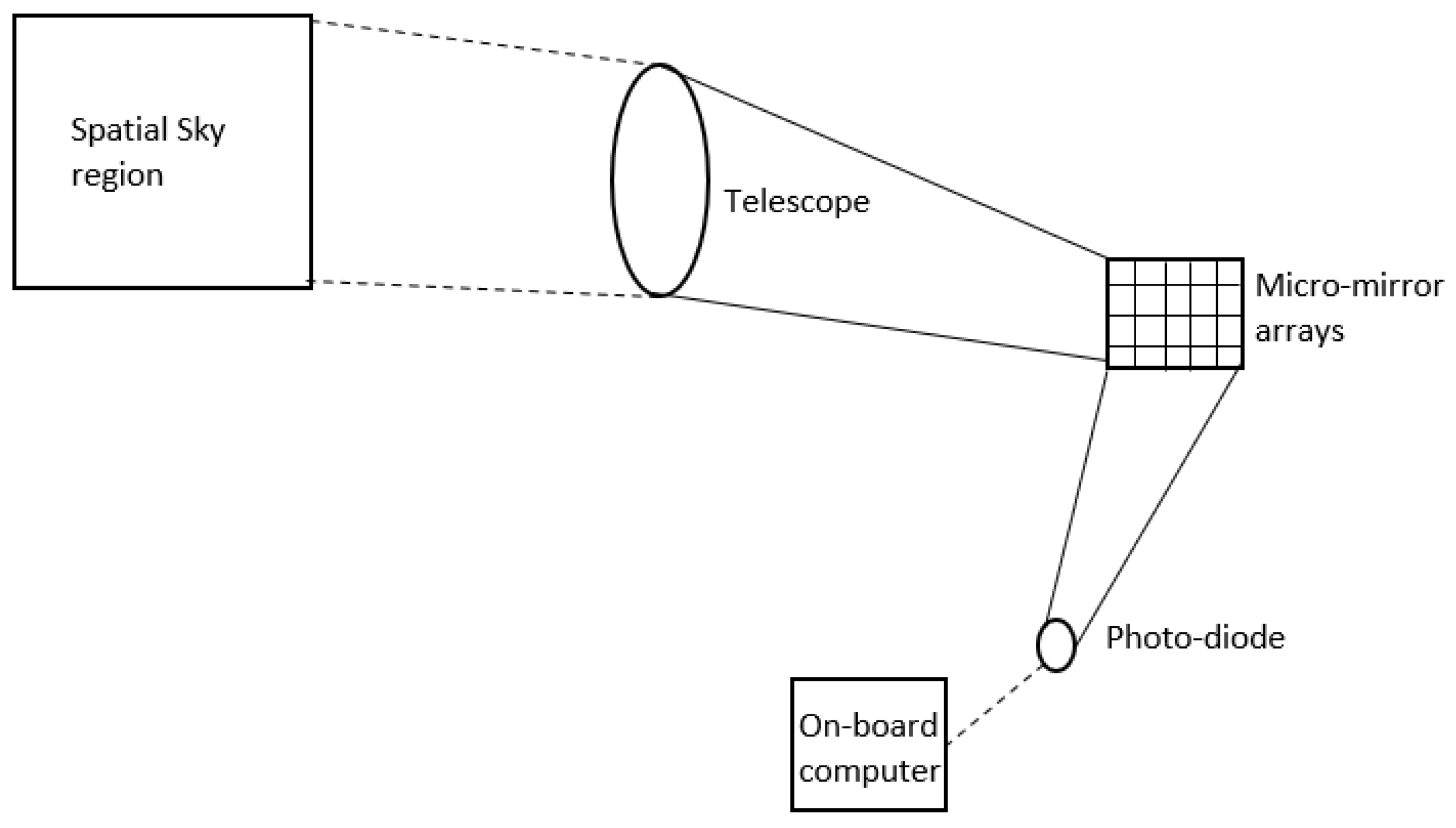
A detector concept for placing a telescope on a Small Satellite can be based off of ASTERIA (Arcsecond Space Telescope Enabling Research in Astrophysics) [20]. ASTERIA is a 6U CubeSat with a telescope aperture of 6.7 cm with a CMOS detector of pixels. For a CS system, our optics would include a telescope, micro-mirror arrays, or any spatial light modulators, as well as a photodiode to acquire the sum total of the reflected light from the micro-mirrors, as shown in Figure 6.
State-of-the-Art Space Flight Instrumentation
In this section, we briefly discuss the current state-of-the-art and the advantages of using a CS detector as compared to traditional detectors.
The front-end-electronics for acquiring photometric measurements will be completely transformed to a novel data acquisition approach using CS techniques, resulting in fewer data samples, eventually putting the image reconstruction load onto computational imaging. Key differences in the optical setup and read-out of traditional detectors and CS based detectors are shown in Table 2.
The current state-of-the-art for microlensing parallax consists of large space observatories, like Nancy Grace Roman Space Telescope detecting an event, then alerting a microlensing event, which is then followed up by a ground observatory. Use of large observatories is very costly. A CS based instrument can detect a microlensing event and capture the complete set. If a parallax measurement is needed, a ground based observatory may be alerted. However, replacing a large observatory with a smaller instrument constellation for parallax detection, which acquires the same resolution science will be a game-changer, causing significant reduction in costs and resources.
5. Simulation Setup
In this section, we discuss the microlensing parameters and the CS parameters used for our simulation modelling.
5.1. Parallax Measurement Setup
In this section, we show effectiveness of CS over a range of and as described in equations. We vary , the space-flight instrument orbital phase to span over a range of values of and . Our microlensing parallax, , is given by Equation (20). From [8], we make the same assumptions of the source being located in the galactic bulge at 4 kpc, lens at 8 kpc with a relative lens-source speed of 200 km/s to obtain the value of .
Hence, in a simple case, with origin as the center of the satellite trajectories, we can write
To generate our parallax measurements, we make the assumptions as in [8]:
- Source is in the galactic bulge: = 8 kpc
- = 4 kpc
We can use Equations (11) and (13) with the given value for in Equation (20). Our simulations vary the value of R and to determine the effect of CS reconstruction on photometric curves with a microlensing parallax. We use R values as shown in Table 3.
The different R values approximately correspond to the type of orbit the constellation could be in: low earth orbit, geosynchronous orbit, and solar orbit, respectively [8,23]. We use eight equally space values. Hence, our results could show the effect for any constellation spaced at the given values: , , , , , , , .
A value of 1 day depicts photometric curves due to free floating planets.
5.2. Compressive Sensing Setup
For CS application, we generate a realistic crowded star field with airy shaped PSF with PSF radius ranging from (1,5) pixel units. For image, we generate star sources. The flux of the star sources ranges from 50 to 5000 units. In our simulations, we use , where m is the number of CS measurements obtained. The number of measurements, m, is a trade-off with the amount of error tolerance desired. We chose m value such that we would keep the average error tolerance to under . A Bernoulli measurement matrix is used, which is varied during each Monte Carlo simulation. For a given R and , we run 100 Monte Carlo simulations at each time sample, t. The number of Monte Carlo simulations chosen are based on two factors: (1) available computational resources and (2) the minimum number needed, such that the average obtained over all Monte Carlo simulations is as close to the “true” average. In order to find the “true” average, we look at the standard deviation of the Monte Carlo simulations to verify that it is as close to 0 as possible. Using 100 Monte Carlo simulations, for , we obtain the average standard deviation over all time samples and values to be . Similarly, for 42,000 and , we obtain the average standard deviation to be and , respectively. Hence, we use 100 Monte Carlo simulations because the standard deviation decreases to a minimal amount across that many number of simulations in our setup. For CS reconstruction, we use the greedy algorithm, orthogonal matching pursuit, as its computational time is relatively less than optimization algorithms.
6. Results
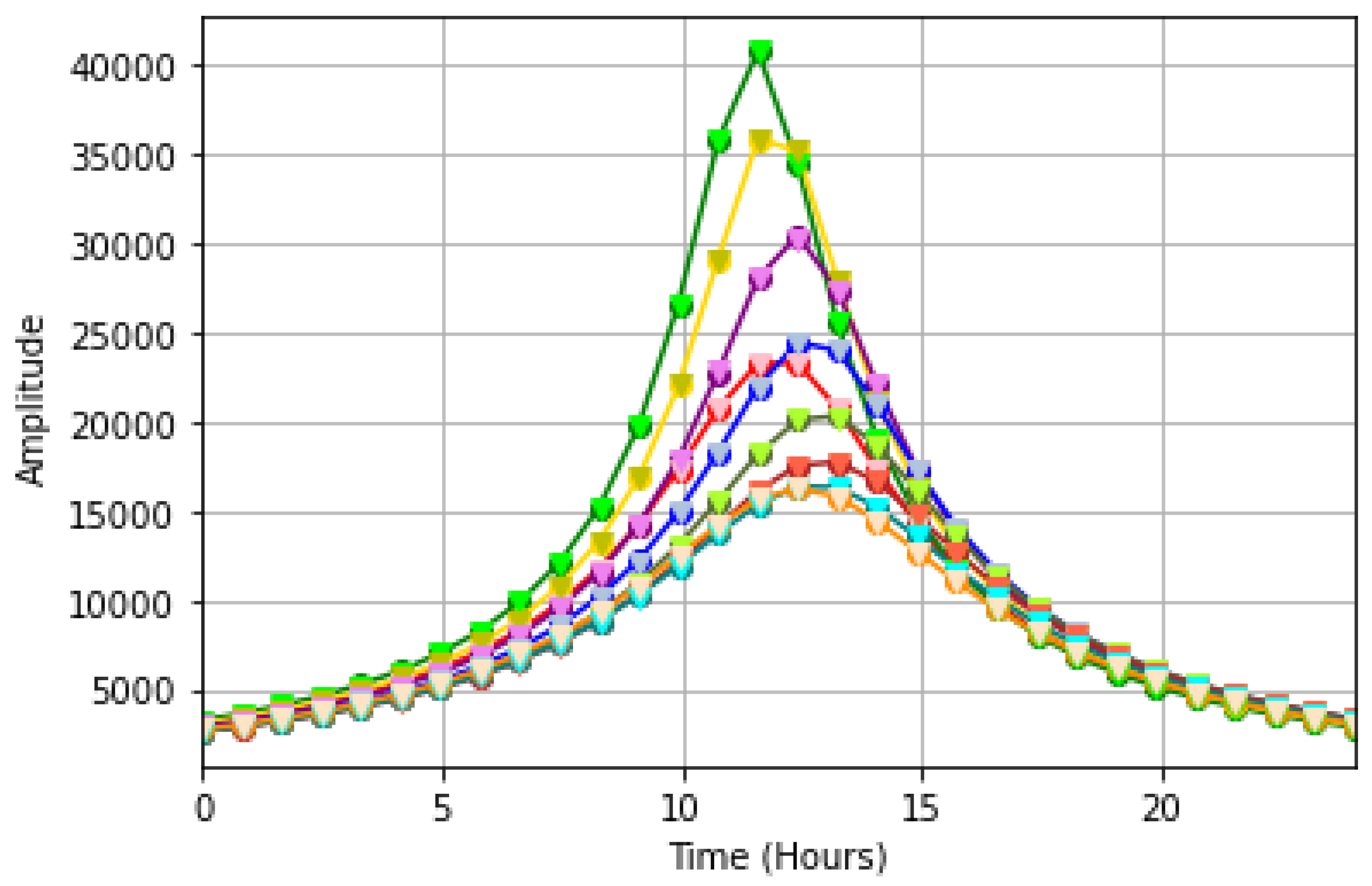
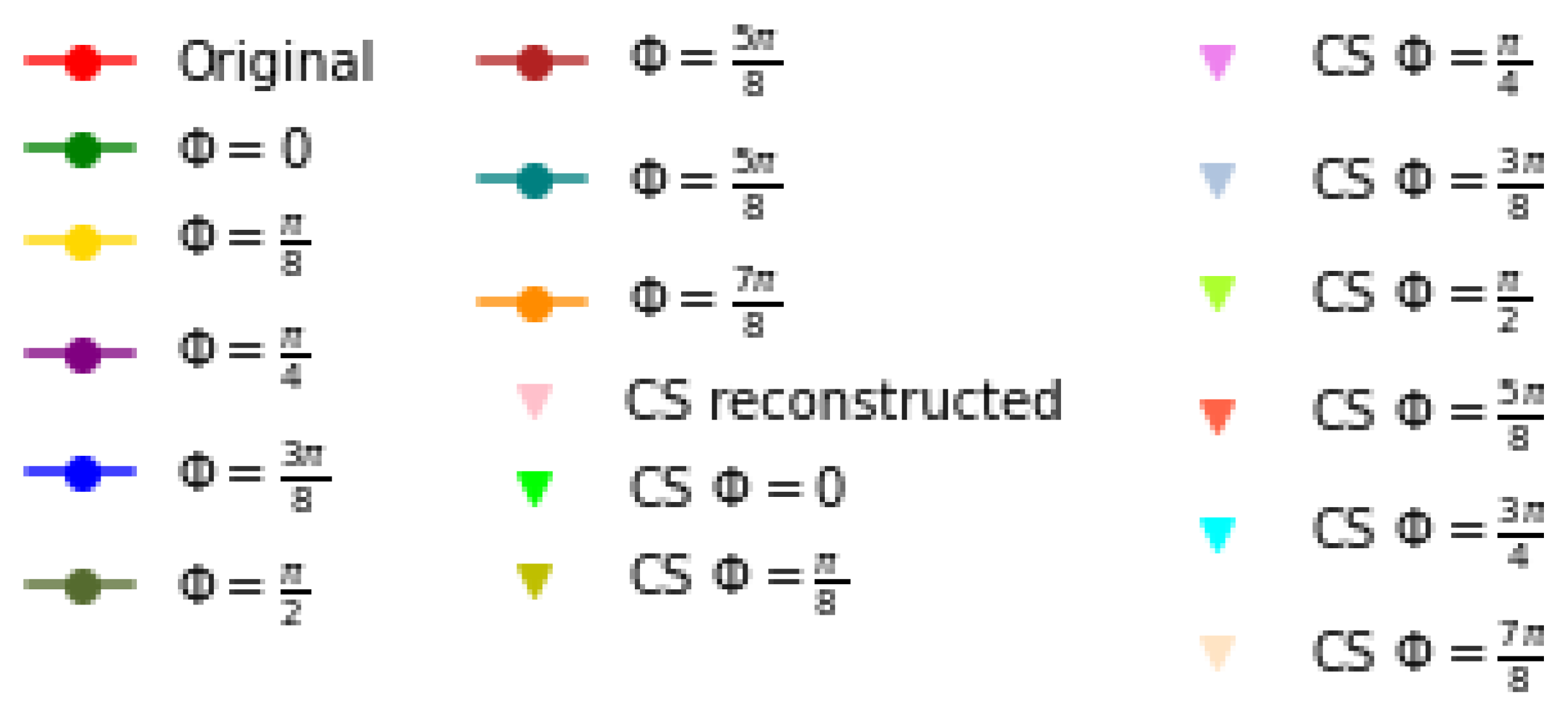
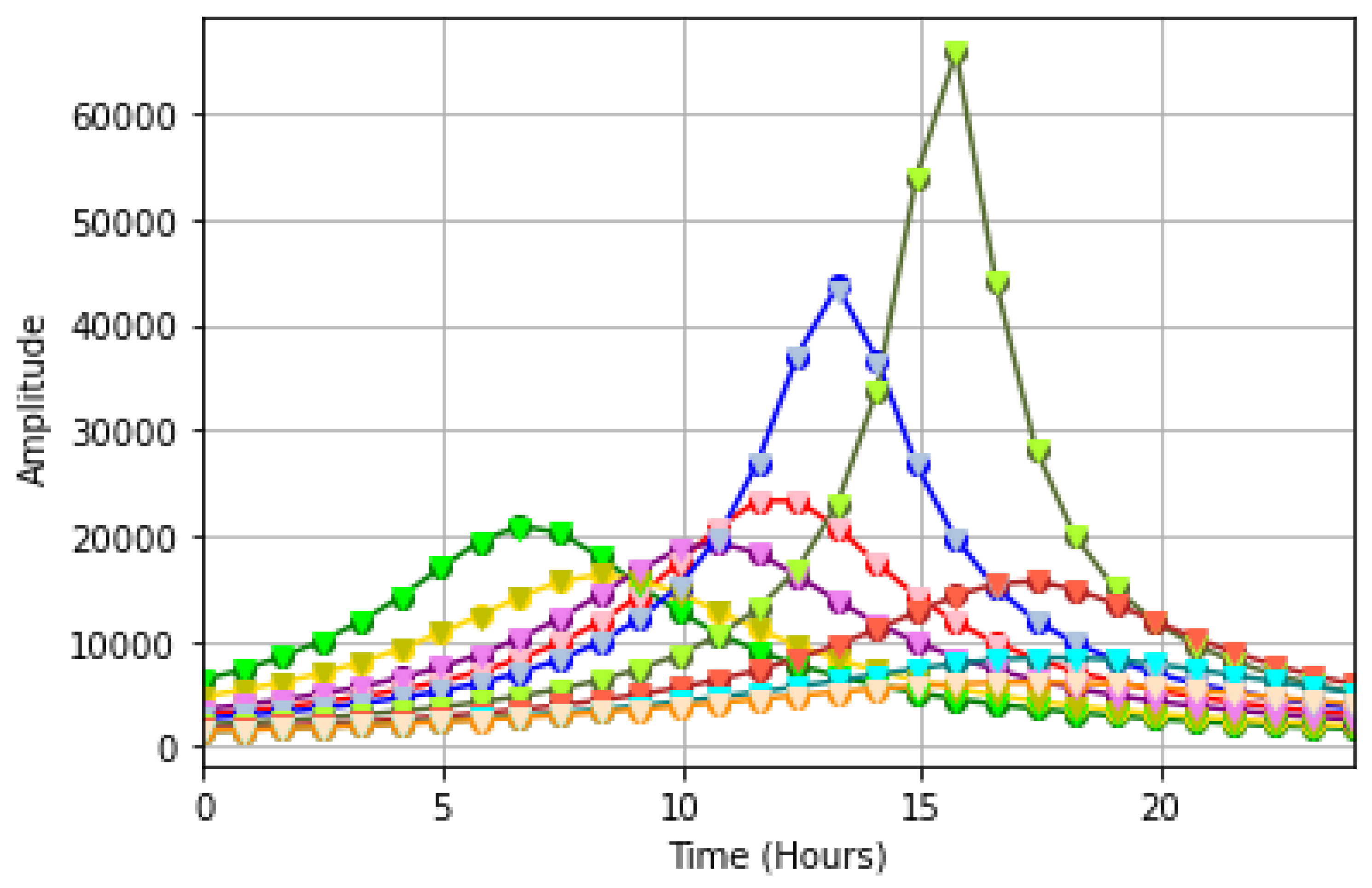
In our first set of simulations for km, we obtain the different parallax light curves for each varying as shown in Figure 7, with the figure legend shown in Figure 8. The photometric curve without parallax, labeled as Original, is also shown for comparison. We perform 100 Monte Carlo simulations for each time sample. For each R value, we show % error in peak magnification value between each parallax photometric curve as well as the difference in time shift for the peak magnification. The average CS reconstruction error for R = 7000 km is shown in Table 4. Table 5 and Table 6 show the error at peak magnification and the time difference in hours at peak magnification for R = 7000 km, respectively. Microlensing parallax provides a , which shows the change in magnification amplitude, as well as a , which shows a change in location. The higher the R value, the greater the .
In the next set of simulations, we use R = 42,000 km. We show the microlensing parallax curves and the photometric curve without a microlensing parallax, shown as Original, in Figure 9, with the figure legend shown in Figure 10. The corresponding errors due to CS reconstruction are shown in Table 7. Table 8 and Table 9 show % error at peak magnification and time difference in hours at peak magnification, respectively.
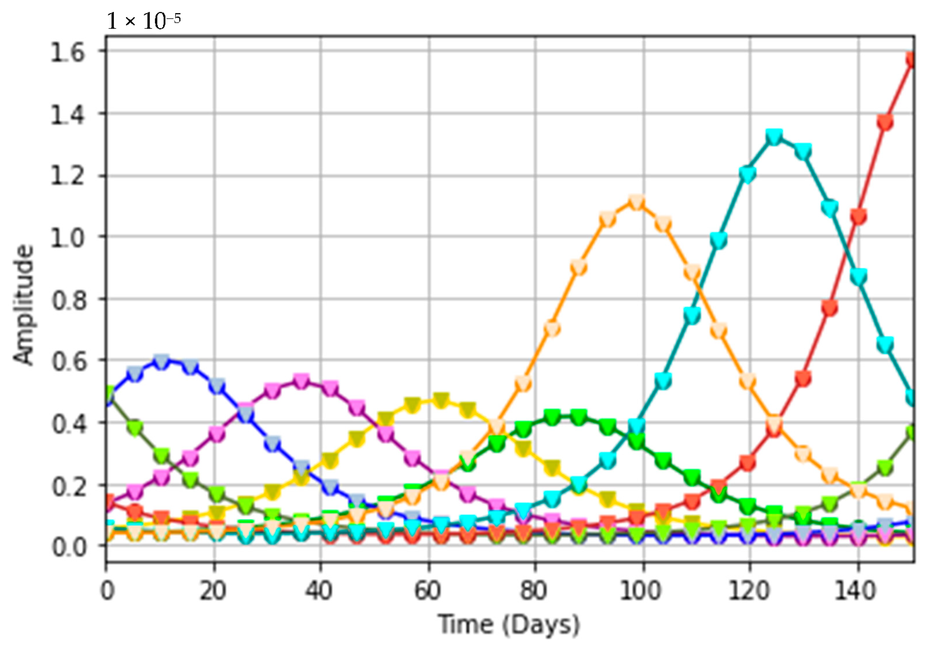
Figure 11 shows the microlensing parallax curves for R = 1 AU. In this figure, we do not show the microlensing curve without parallax (Original curve in Figure 7 and Figure 9) for comparison, as the in and are significantly high and will not be clearly readable with the given sampling cadence and observation window. Figure 12 is the corresponding legend. In Table 10, we show the % error due to CS reconstruction in the photometric curves. Table 11 and Table 12 show % error at peak magnification and time difference in days at peak magnification, respectively.
For all three categories, as shown in Figure 7, Figure 9, and Figure 11, the CS reconstructed curves and original curves overlap, as CS reconstruction nearly perfectly reconstructs the original curve. Average CS reconstruction % error over all samples for the photometric curve with no microlensing parallax was , and the average % error at was .
Our results show that there is no significant error for a microlensing parallax event using CS techniques. For all the photometric curves, the average error is less than for all CS reconstructed curves and less than at peak magnification time.
From our simulations, we note that the parallax curves get more distinguished for higher R values, that is, the time separation and amplitude separation between the photometric curves is higher. From our simulations, we show that the error due to CS reconstruction is less than the error between any two microlens parallax curves. However, we can use Table 5, Table 8 and Table 11 as a basis to determine the optimal orbital phases to choose for satellite placement. Although CS reconstruction results show average error within the % error for the two curves, a better placement, if using less than eight satellites, would be to choose orbital phases which have a greater microlensing detectability.
7. Data Volume and Resources
In this section, we perform a comparison analysis of using traditional detectors versus CS based detectors.
- 1
- Data volume storageUsing a image, with a 14-bit ADC resolution, we would expect the total data volume to be:
Traditional Detector CS detector 14 bits × 14 bits × We would make the assumption that the photodetector is not saturated with the ADC bit resolution needed to sample. Without data compression, we will need to transfer bits/ FOV using a traditional detector. Using CS approach for measurements, we can will need to transmit bits/ FOV. - 2
- Computational resourcesOn-board computation will consist of programming the spatial modulator and storing the size acquired data for each spatial image. To compare this with a traditional detector system, we would require computational resources for compressing data on-board, in order to be accommodated in the data down-link bandwidth.In terms of on-board Field Programmable Gate Array (FPGA) resources for each of the modules listed in Table 13, we would expect a similar amount of logic gates, except for item 3. There are different methods for implementing data compression, including compression algorithms and pixel averaging [24,25]. For CS detectors, spatial modulation implementation will depend on the spatial modulator used. In addition, we would require either storage or generation and transmission of the spatial modulation matrix (CS measurement matrix) on-board. The on-board storage needed for traditional detectors would be significantly higher than storage needed for CS architecture modules.
- 3
- OpticsA traditional detector consists of a telescope and a detector, typically a CCD camera. In the case for CS, we would need a telescope, as well as lenses, to focus the light on a spatial modulator device, such as a DMD array, followed by a photodetector. However, lensless cameras for CS applications have been implemented [16,17,18] and would need to be studied for a SmallSat type instrument. The optical path required to implement the detector system will be further studied in future work.
8. Conclusions
We simulated microlensing parallax curves with different orbital phases using CS techniques. Our CS simulation results show an error of less than over all time samples and an average error of less than at , while using of traditional detector measurements for microlensing parallax light curves with a range of from [0, ]. Despite different microlensing parallaxes at the three orbital radii generating different photometric curves with significant difference in flux magnitude, CS worked well for all the cases. The CS error at peak magnification for R = 7000 km, 42,000 km, and 1 AU, at each value is less than the error between the parallax curve generated with that particular value and any other parallax curve generated using the value ranges. This shows that CS reconstruction should not cause any significant errors in detection of a microlensing parallax curve for any given value. Using CS, we can significantly reduce the data storage volume, as well as data downlink bandwidth—both of which can be a limitation for SmallSat type instruments. CS shows potential for implementation in a SmallSat constellation for detecting microlensing parallax events.
Author Contributions
Conceptualization, A.K.-P. and R.K.B.; methodology, A.K.-P.; writing—original draft preparation, A.K.-P.; writing—review and editing, R.K.B.; supervision, T.M. and R.K.B.; All authors have read and agreed to the published version of the manuscript.
Funding
This research received no external funding.
Institutional Review Board Statement
Not applicable.
Informed Consent Statement
Not applicable.
Data Availability Statement
We have used simulated data using simulation parameters described in this work. This study has not used any publicly available datasets.
Conflicts of Interest
The authors declare no conflict of interest.
Abbreviations
The following abbreviations are used in this manuscript:
| CS | Compressive Sensing |
| SmallSat | Small Satellite |
| FOV | Field-of-View |
| ASTERIA | Arcsecond Space Telescope Enabling Research in Astrophysics |
| FPGA | Field Programmable Gate Array |
| DMD | Digital Micro-mirror Device |
| ADC | Analog-to-Digital Converter |
References
- Eldar, Y.C.; Kutyniok, G. (Eds.) Compressed Sensing: Theory and Applications; Cambridge University Press: Cambridge, UK, 2012. [Google Scholar]
- Candès, E.J.; Wakin, M.B. An introduction to compressive sampling [a sensing/sampling paradigm that goes against the common knowledge in data acquisition]. IEEE Signal Process. Mag. 2008, 25, 21–30. [Google Scholar]
- Candes, E.; Romberg, J. Sparsity and incoherence in compressive sampling. Inverse Probl. 2007, 23, 969. [Google Scholar] [CrossRef]
- Bobin, J.; Starck, J.L.; Ottensamer, R. Compressed sensing in astronomy. IEEE J. Sel. Top. Signal Process. 2008, 2, 718–726. [Google Scholar] [CrossRef]
- Seager, S. Exoplanets; University of Arizona Press: Tucson, AZ, USA, 2010. [Google Scholar]
- Gould, A. “Rigorous” Rich Argument in Microlensing Parallax. arXiv 2020, arXiv:2002.00947. [Google Scholar]
- Yee, J.C. Lens Masses and Distances from Microlens Parallax and Flux. Astrophys. J. Lett. 2015, 814, L11. [Google Scholar] [CrossRef]
- Bachelet, E.; Hinse, T.C.; Street, R. Measuring the Microlensing Parallax from Various Space Observatories. Astron. J. 2018, 155, 191. [Google Scholar] [CrossRef]
- Lee, C.-H. Microlensing and Its Degeneracy Breakers: Parallax, Finite Source, High-Resolution Imaging, and Astrometry. Universe 2017, 3, 53. [Google Scholar] [CrossRef]
- Smith, M.C.; Mao, S.; Paczyński, B. Acceleration and parallax effects in gravitational microlensing. Mon. Not. R. Astron. Soc. 2003, 339, 925–936. [Google Scholar] [CrossRef]
- Bramich, D.M. A new algorithm for difference image analysis. Mon. Not. R. Astron. Soc. Lett. 2008, 386, L77–L81. [Google Scholar] [CrossRef]
- Wakin, M.B.; Laska, J.N.; Duarte, M.F.; Baron, D.; Sarvotham, S.; Takhar, D.; Kelly, K.F.; Baraniuk, R.G. An architecture for compressive imaging. In Proceedings of the 2006 International Conference on Image Processing, Atlanta, GA, USA, 8–11 October 2006; IEEE: Piscataway, NJ, USA, 2006. [Google Scholar]
- Guzzi, D.; Coluccia, G.; Labate, D.; Lastri, C.; Magli, E.; Nardino, V.; Palombi, L.; Pippi, I.; Coltuc, D.; Marchi, A.Z.; et al. Optical compressive sensing technologies for space applications: Instrumental concepts and performance analysis. In Proceedings of the International Conference on Space Optics—ICSO 2018, Chania, Greece, 9–12 October 2018; p. 111806B. [Google Scholar]
- Frederic, Z.; Lanzoni, P.; Tangen, K. Micromirror arrays for multi-object spectroscopy in space. In Proceedings of the International Conference on Space Optics—ICSO 2010, Rhodes Island, Greece, 4–8 October 2010; International Society for Optics and Photonics: Bellingham, WA, USA, 2019; Volume 10565. [Google Scholar]
- Xiao, L.L.; Liu, K.; Han, D.P.; Liu, J.Y. A compressed sensing approach for enhancing infrared imaging resolution. Opt. Laser Technol. 2012, 44, 2354–2360. [Google Scholar] [CrossRef]
- Zhang, Z.; Su, Z.; Deng, Q.; Ye, J.; Peng, J.; Zhong, J. Lensless single-pixel imaging by using LCD: Application to small-size and multi-functional scanner. Opt. Express 2019, 27, 3731–3745. [Google Scholar] [CrossRef] [PubMed]
- Kuusela, T.A. Single-pixel camera. Am. J. Phys. 2019, 87, 846–850. [Google Scholar] [CrossRef]
- Gang, H.; Hong, J.; Matthews, K.; Wilford, P. Lensless imaging by compressive sensing. In Proceedings of the 2013 IEEE International Conference on Image Processing, Melbourne, VIC, Australia, 15–18 September 2013; IEEE: Piscataway, NJ, USA, 2013. [Google Scholar]
- Mróz, P.; Poleski, R.; Gould, A.; Udalski, A.; Sumi, T.; Szymański, M.K.; Soszyński, I.; Pietrukowicz, P.; Kozłowski, S.; Skowron, J.; et al. A terrestrial-mass rogue planet candidate detected in the shortest-timescale microlensing event. Astrophys. J. Lett. 2020, 903, L11. [Google Scholar] [CrossRef]
- Krishnamurthy, A.; Knapp, M.; Günther, M.N.; Daylan, T.; Demory, B.; Seager, S.; Bailey, V.P.; Smith, M.W.; Pong, C.M.; Hughes, K.; et al. Transit Search for Exoplanets around Alpha Centauri A and B with ASTERIA. Astron. J. 2021, 161, 275. [Google Scholar] [CrossRef]
- Gould, A. A natural formalism for microlensing. Astrophys. J. 2000, 542, 785. [Google Scholar] [CrossRef]
- Yan, S.; Zhu, W. Measuring microlensing parallax via simultaneous observations from Chinese Space Station Telescope and Roman Telescope. Res. Astron. Astrophys. 2021, 22, 025006. [Google Scholar] [CrossRef]
- Mogavero, F.; Beaulieu, J.P. Microlensing planet detection via geosynchronous and low Earth orbit satellites. Astron. Astrophys. 2016, 585, A62. [Google Scholar] [CrossRef]
- Anuradha, D.; Bhuvaneswari, S. A detailed review on the prominent compression methods used for reducing the data volume of big data. Ann. Data Sci. 2016, 3, 47–62. [Google Scholar] [CrossRef]
- Yaman, D.; Kumar, V.; Singh, R.S. Comprehensive review of hyperspectral image compression algorithms. Opt. Eng. 2020, 59, 090902. [Google Scholar]
Figure 1.
CS Architecture. The blue block represents CS data acquisition which can be performed on-board a spaceflight instrument, while the orange blocks represent computations which can be performed on the ground. Image differencing can also be performed on-board to further reduce data volume.
Figure 1.
CS Architecture. The blue block represents CS data acquisition which can be performed on-board a spaceflight instrument, while the orange blocks represent computations which can be performed on the ground. Image differencing can also be performed on-board to further reduce data volume.
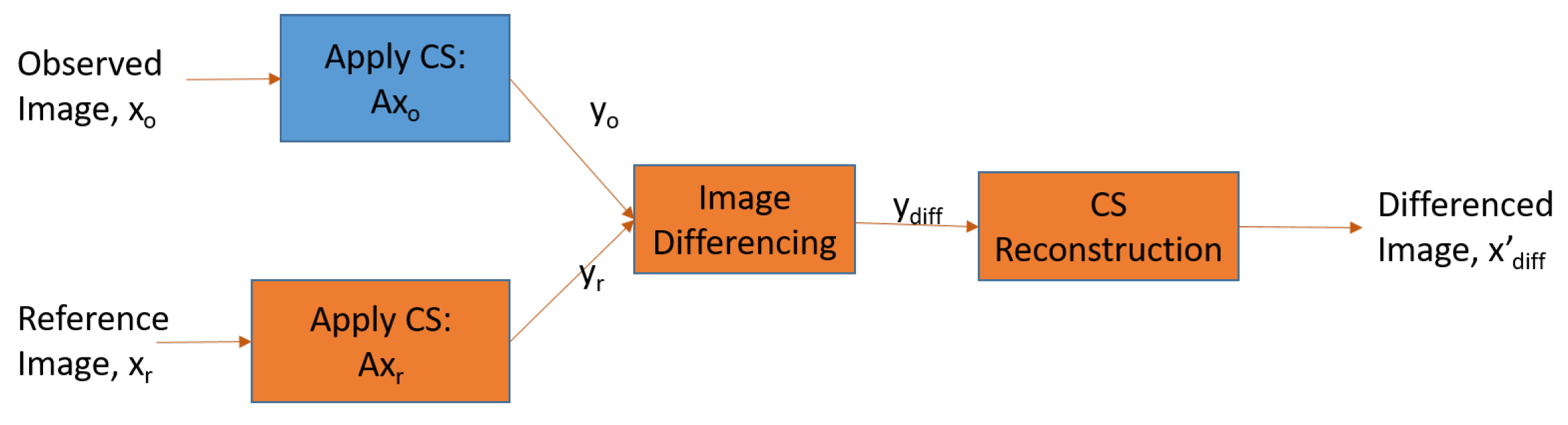
Figure 2.
Sample reference image.

Figure 3.
Sample observed image.

Figure 4.
Sample differenced image.

Figure 5.
A diagram of satellite constellations observing the same spatial region in order to capture a microlensing parallax of any microlensing event occurring the given field-of-view. X represents a satellite with a CS detector system.
Figure 5.
A diagram of satellite constellations observing the same spatial region in order to capture a microlensing parallax of any microlensing event occurring the given field-of-view. X represents a satellite with a CS detector system.

Figure 6.
A potential CS implementation of the detector system using a telescope to acquire the light from the spatial region, a set of micro-mirror arrays to reflect light using CS projection methods, and a photodiode to capture a single measurement of the total reflected light.
Figure 6.
A potential CS implementation of the detector system using a telescope to acquire the light from the spatial region, a set of micro-mirror arrays to reflect light using CS projection methods, and a photodiode to capture a single measurement of the total reflected light.

Figure 7.
Photometric curves generated by different parallax values, shown with its corresponding CS reconstructed curve for R = 7000 km.
Figure 7.
Photometric curves generated by different parallax values, shown with its corresponding CS reconstructed curve for R = 7000 km.

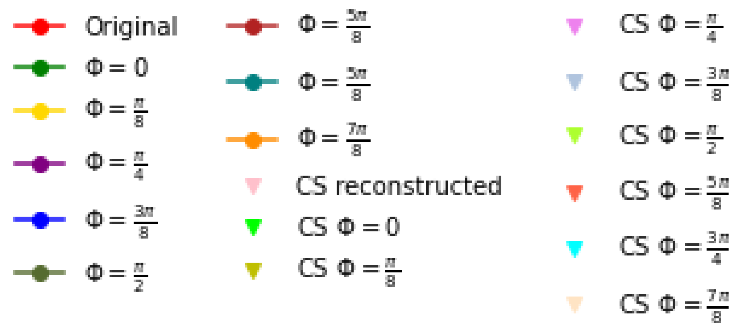
Figure 8.
Legend for Figure 7.
Figure 8.
Legend for Figure 7.

Figure 9.
Photometric curves generated by different parallax values, shown with its corresponding CS reconstructed curve for R = 42,000 km. The original photometric curve without any microlensing effects is shown in red for comparison.
Figure 9.
Photometric curves generated by different parallax values, shown with its corresponding CS reconstructed curve for R = 42,000 km. The original photometric curve without any microlensing effects is shown in red for comparison.

Figure 10.
Legend for Figure 9.
Figure 10.
Legend for Figure 9.

Figure 11.
Photometric curves generated by different parallax values, shown with its corresponding CS reconstructed curve for R = 1 AU. The magnification is significantly lower because the differenced image is reconstructed using our CS technique, and the in both and is significantly high.
Figure 11.
Photometric curves generated by different parallax values, shown with its corresponding CS reconstructed curve for R = 1 AU. The magnification is significantly lower because the differenced image is reconstructed using our CS technique, and the in both and is significantly high.

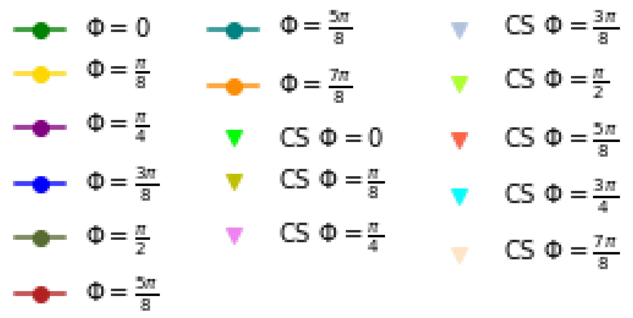
Figure 12.
Legend for Figure 11.
Figure 12.
Legend for Figure 11.


Table 1.
Microlensing parameter definitions obtained from a photometric curve.
| Parameter | Definition |
|---|---|
| Time of peak magnification | |
| Einstein ring crossing time: | |
| Impact parameter in units of | |
| Microlensing source star flux | |
| Microlensing source star blended flux |
Table 2.
Comparison between traditional detectors and CS detectors.
| Traditional Detectors | CS Detectors |
|---|---|
| CCD Detectors | Typically designed with spatial light modulators and photodiode |
| Pixel by pixel readout of the image | Total power reflected from the matrix projected onto the image is measured |
| Digitization of each pixel readout | Digitization of the total power read |
Table 3.
Simulation setup parameters.
| R | Cadence | Observation Time | |
|---|---|---|---|
| 7000 km | 1 day | 48 min | 1 day |
| 42,000 km | 1 day | 48 min | 1 day |
| 1 AU | 1 day | 5.02 days | 150.5 days |
Table 4.
Percent Error for CS reconstruction for each for R = 7000 km. The second row shows average % error over all time samples, the third row shows average % error at peak magnification, and the last row shows the standard deviation of the % error at peak magnification.
Table 4.
Percent Error for CS reconstruction for each for R = 7000 km. The second row shows average % error over all time samples, the third row shows average % error at peak magnification, and the last row shows the standard deviation of the % error at peak magnification.
| 0 | ||||||||
|---|---|---|---|---|---|---|---|---|
| Avg % Err | 0.175 | 0.230 | 0.088 | 0.109 | 0.163 | 0.161 | 0.240 | 0.098 |
| Avg % Err at peak | 0.075 | 0.06 | 1.07 | 0.068 | 1.09 | 0.076 | 0.081 | 0.073 |
| Std dev. % Err at peak | 0.057 | 0.064 | 9.94 | 0.056 | 9.94 | 0.086 | 0.070 | 0.068 |
Table 5.
Percent error at peak magnification over 100 Monte Carlo simulations, between a microlensing photometric curve with shown in the first row, compared to the photometric curve with in the first column. Error values for R = 7000 km. Values in bold underline show where % error between the two curves is less than .
| 0 | ||||||||
|---|---|---|---|---|---|---|---|---|
| 0 | - | 12.0 | 25.3 | 40.0 | 50.2 | 56.5 | 59.8 | 60.1 |
| 13.6 | - | 15.2 | 31.8 | 43.4 | 50.6 | 54.4 | 54.7 | |
| 33.9 | 17.9 | - | 19.6 | 33.3 | 41.7 | 46.2 | 46.6 | |
| 66.7 | 46.7 | 24.5 | - | 16.9 | 27.5 | 33.1 | 33.5 | |
| 101 | 76.6 | 49.8 | 20.4 | - | 12.7 | 19.4 | 20.0 | |
| 130 | 102 | 71.6 | 37.9 | 14.5 | - | 7.72 | 8.34 | |
| 149 | 119 | 85.9 | 49.4 | 24.1 | 8.36 | - | 0.674 | |
| 151 | 121 | 87.2 | 50.4 | 24.9 | 9.10 | 0.679 | - |
Table 6.
Time difference in Hours at peak magnification between a microlensing photometric curve with shown in the first row, compared to the photometric curve with in the first column. R = 7000 km.
Table 6.
Time difference in Hours at peak magnification between a microlensing photometric curve with shown in the first row, compared to the photometric curve with in the first column. R = 7000 km.
| 0 | ||||||||
|---|---|---|---|---|---|---|---|---|
| 0 | - | 0 | 0.828 | 0.828 | 1.66 | 1.66 | 0.828 | 0.828 |
| 0 | - | 0.828 | 0.828 | 1.66 | 1.66 | 0.828 | 0.828 | |
| 0.828 | 0.828 | - | 0 | 0.828 | 0.828 | 0. | 0 | |
| 0.828 | 0.828 | 0 | - | 0.828 | 0.828 | 0 | 0 | |
| 1.66 | 1.66 | 0.828 | 0.828 | - | 0 | 0.828 | 0.828 | |
| 1.66 | 1.66 | 0.828 | 0.828 | 0 | - | 0.828 | 0.828 | |
| 0.828 | 0.828 | 0 | 0 | 0.828 | 0.828 | - | 0 | |
| 0.828 | 0.828 | 0 | 0 | 0.828 | 0.828 | 0 | - |
Table 7.
Percent Error for CS reconstruction for each for R = 42,000 km. The second row shows average % error over all time samples, the third row shows average % error at , and the last row shows the standard deviation of the % error at .
Table 7.
Percent Error for CS reconstruction for each for R = 42,000 km. The second row shows average % error over all time samples, the third row shows average % error at , and the last row shows the standard deviation of the % error at .
| 0 | ||||||||
|---|---|---|---|---|---|---|---|---|
| Avg % Err | 0.108 | 0.110 | 0.182 | 0.110 | 0.191 | 0.208 | 0.173 | 0.201 |
| Avg % Err at peak | 1.07 | 0.059 | 0.091 | 1.07 | 0.086 | 0.063 | 0.062 | 0.071 |
| Std dev. % Err at peak | 9.94 | 0.041 | 0.205 | 9.94 | 0.094 | 0.049 | 0.062 | 0.057 |
Table 8.
Percent error at peak magnification between a microlensing photometric curve with shown in the first row, compared to the photometric curve with in the first column. Error values for R = 42,000 km. Values in bold underline show where % error between the two curves is less than .
Table 8.
Percent error at peak magnification between a microlensing photometric curve with shown in the first row, compared to the photometric curve with in the first column. Error values for R = 42,000 km. Values in bold underline show where % error between the two curves is less than .
| 0 | ||||||||
|---|---|---|---|---|---|---|---|---|
| 0 | - | 22.1 | 7.50 | 109 | 215 | 25.1 | 59.7 | 70.9 |
| 28.3 | - | 18.7 | 168 | 305 | 3.85 | 48.3 | 62.6 | |
| 8.11 | 15.8 | - | 126 | 241 | 19.0 | 56.5 | 68.5 | |
| 52.1 | 62.7 | 55.7 | - | 51.0 | 64.1 | 80.7 | 86.1 | |
| 68.3 | 75.3 | 70.7 | 33.8 | - | 76.2 | 87.2 | 90.8 | |
| 33.5 | 4.00 | 23.5 | 179 | 321 | - | 46.2 | 61.1 | |
| 148 | 93.4 | 130 | 418 | 682 | 86.0 | - | 27.7 | |
| 243 | 168 | 218 | 617 | 982 | 157 | 38.3 | - |
Table 9.
Time difference in Hours at peak magnification between microlensing photometric curve with shown in the first row, compared to the photometric curve with in the first column. Error values for R = 42,000 km.
Table 9.
Time difference in Hours at peak magnification between microlensing photometric curve with shown in the first row, compared to the photometric curve with in the first column. Error values for R = 42,000 km.
| 0 | ||||||||
|---|---|---|---|---|---|---|---|---|
| 0 | - | 1.66 | 4.14 | 6.62 | 9.10 | 10.8 | 10.8 | 10.8 |
| 1.66 | - | 2.48 | 4.97 | 7.45 | 9.10 | 9.10 | 9.10 | |
| 4.14 | 2.48 | - | 2.48 | 4.97 | 6.62 | 6.62 | 6.62 | |
| 6.62 | 4.97 | 2.48 | - | 2.48 | 4.14 | 4.14 | 4.14 | |
| 9.10 | 7.45 | 4.97 | 2.48 | - | 1.66 | 1.66 | 1.66 | |
| 10.8 | 9.10 | 6.62 | 4.14 | 1.66 | - | 0 | 0 | |
| 10.8 | 9.10 | 6.62 | 4.14 | 1.66 | 0 | - | 0 | |
| 10.8 | 9.10 | 6.62 | 4.14 | 1.66 | 0 | 0 | - |
Table 10.
Percent Error for CS reconstruction for each for R = 1 AU. The second row shows average % error over all time samples, the third row shows average % error at the peak of each curve, and the last row shows the standard deviation of the % error at the peak.
Table 10.
Percent Error for CS reconstruction for each for R = 1 AU. The second row shows average % error over all time samples, the third row shows average % error at the peak of each curve, and the last row shows the standard deviation of the % error at the peak.
| 0 | ||||||||
|---|---|---|---|---|---|---|---|---|
| Avg % Err | 0.437 | 0.441 | 0.633 | 0.743 | 0.621 | 0.348 | 0.616 | 0.582 |
| Avg % Err at peak | 0.186 | 0.192 | 0.192 | 0.194 | 0.183 | 0.119 | 0.106 | 0.117 |
| Std dev. % Err at peak | 0.146 | 0.190 | 0.178 | 0.183 | 0.137 | 0.287 | 0.092 | 0.083 |
Table 11.
Percent error at peak between a microlensing photometric curve with shown in the first row, compared to the photometric curve with in the first column. Error values for R = 1 AU. Values in bold underline show where % error between the two curves is less than .
Table 11.
Percent error at peak between a microlensing photometric curve with shown in the first row, compared to the photometric curve with in the first column. Error values for R = 1 AU. Values in bold underline show where % error between the two curves is less than .
| 0 | ||||||||
|---|---|---|---|---|---|---|---|---|
| 0 | - | 12.7 | 27.2 | 43.7 | 18.7 | 276 | 217 | 167 |
| 11.3 | - | 12.8 | 27.5 | 5.34 | 234 | 181 | 137 | |
| 21.4 | 11.4 | - | 13.0 | 6.65 | 196 | 149 | 110 | |
| 30.4 | 21.5 | 11.5 | - | 17.4 | 162 | 121 | 85.6 | |
| 15.8 | 5.07 | 7.12 | 21.0 | - | 217 | 167 | 125 | |
| 73.4 | 70.0 | 66.2 | 61.8 | 68.4 | - | 15.7 | 29.1 | |
| 68.5 | 64.4 | 59.9 | 54.7 | 62.5 | 18.6 | - | 15.9 | |
| 62.5 | 57.7 | 52.3 | 46.1 | 55.5 | 41.0 | 18.9 | - |
Table 12.
Time difference in Days at peak between a microlensing photometric curve with shown in the first row, compared to the photometric curve with in the first column. Error values for R = 1 AU. Values in bold underline show where % error between the two curves is less than .
Table 12.
Time difference in Days at peak between a microlensing photometric curve with shown in the first row, compared to the photometric curve with in the first column. Error values for R = 1 AU. Values in bold underline show where % error between the two curves is less than .
| 0 | ||||||||
|---|---|---|---|---|---|---|---|---|
| 0 | - | 25.9 | 51.9 | 77.8 | 88.2 | 62.3 | 36.3 | 10.4 |
| 25.9 | - | 25.9 | 51.9 | 62.3 | 88.2 | 62.3 | 36.3 | |
| 51.9 | 25.9 | - | 25.9 | 36.3 | 114 | 88.2 | 62.3 | |
| 77.8 | 51.9 | 25.9 | - | 10.4 | 140 | 114 | 88.2 | |
| 88.2 | 62.3 | 36.3 | 10.4 | - | 151 | 125 | 98.6 | |
| 62.3 | 88.2 | 114 | 140 | 151 | - | 25.9 | 51.9 | |
| 36.3 | 62.3 | 88.2 | 114 | 125 | 25.9 | - | 25.9 | |
| 10.4 | 36.3 | 62.3 | 88.2 | 98.6 | 51.9 | 25.9 | - |
Table 13.
FPGA modules comparison for a traditional detector and CS based detector.
| Traditional Detector | CS Detector | |
|---|---|---|
| 1 | Data acquisition (ADC) interface | Data acquisition (ADC) interface |
| 2 | Data storage module | Data storage module |
| 3 | Data compression | Spatial modulation implementation |
| 4 | Data packetization and transmission | Data packetization and transmission |
Publisher’s Note: MDPI stays neutral with regard to jurisdictional claims in published maps and institutional affiliations. |
© 2022 by the authors. Licensee MDPI, Basel, Switzerland. This article is an open access article distributed under the terms and conditions of the Creative Commons Attribution (CC BY) license (https://creativecommons.org/licenses/by/4.0/).
Share and Cite
MDPI and ACS Style
Korde-Patel, A.; Barry, R.K.; Mohsenin, T. Compressive Sensing Based Space Flight Instrument Constellation for Measuring Gravitational Microlensing Parallax. Signals 2022, 3, 559-576. https://doi.org/10.3390/signals3030034
AMA Style
Korde-Patel A, Barry RK, Mohsenin T. Compressive Sensing Based Space Flight Instrument Constellation for Measuring Gravitational Microlensing Parallax. Signals. 2022; 3(3):559-576. https://doi.org/10.3390/signals3030034
Chicago/Turabian StyleKorde-Patel, Asmita, Richard K. Barry, and Tinoosh Mohsenin. 2022. "Compressive Sensing Based Space Flight Instrument Constellation for Measuring Gravitational Microlensing Parallax" Signals 3, no. 3: 559-576. https://doi.org/10.3390/signals3030034