
Saliency-Guided Local Full-Reference Image Quality Assessment


Abstract
:1. Introduction
1.1. Motivation and Contributions
1.2. Organization of the Paper
2. Related Work
3. Proposed Method
3.1. ESSIM Method
3.2. SG-ESSIM Method
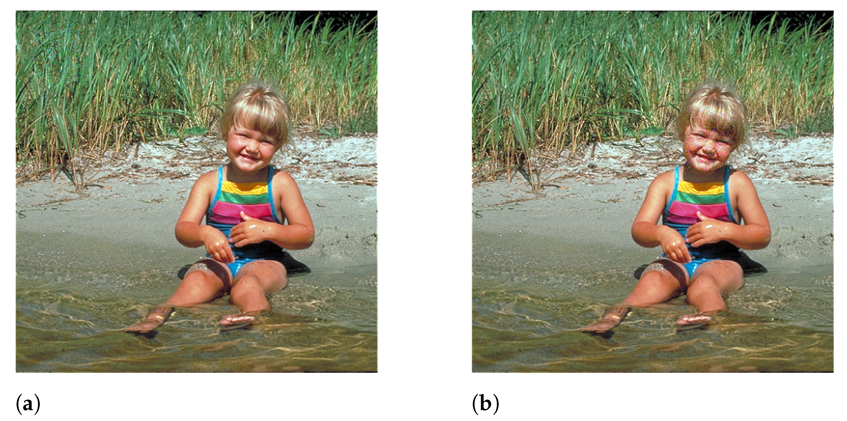
4. Materials
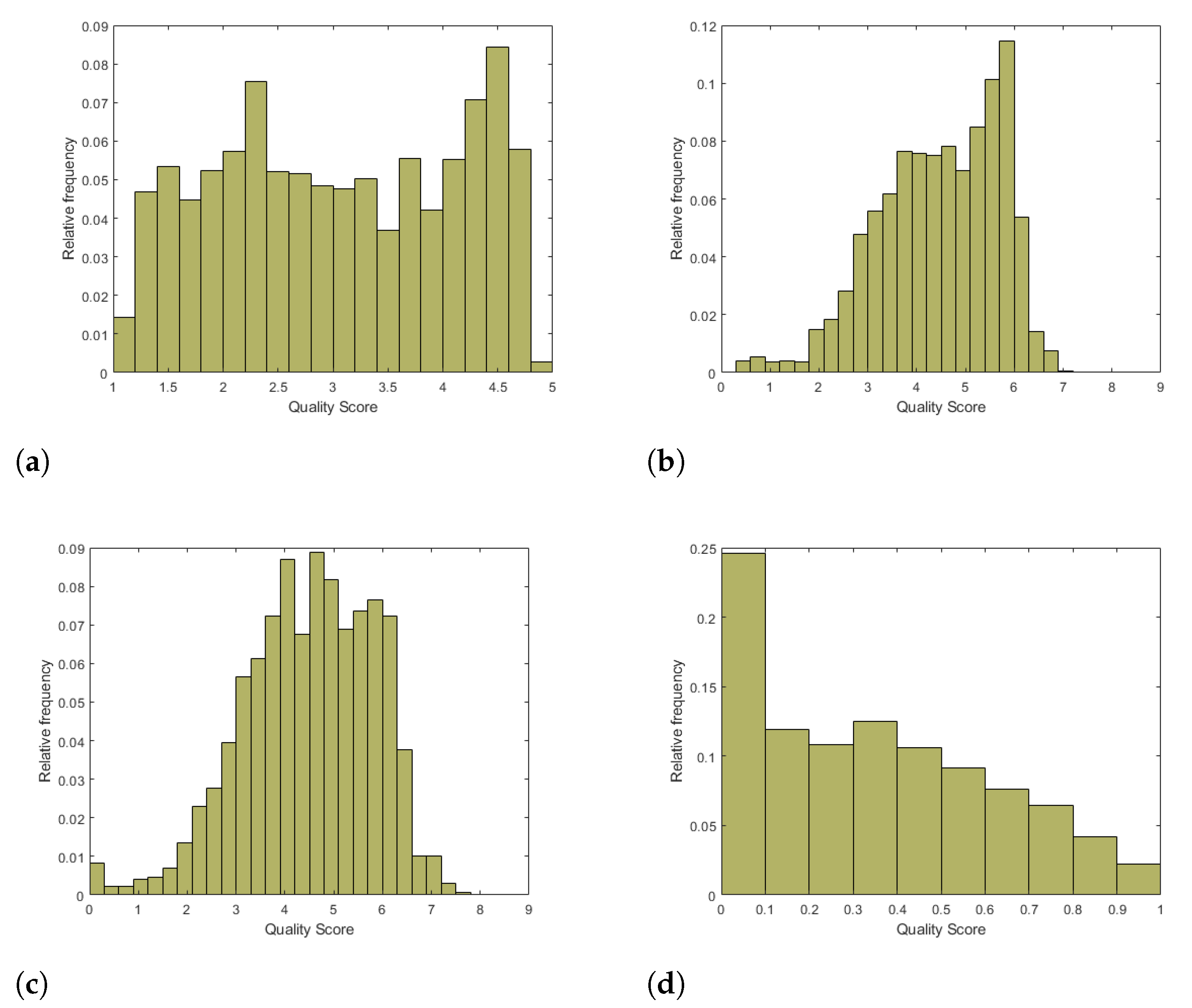
4.1. Databases
4.2. Evaluation Metrics and Protocol
4.3. Implementation Details
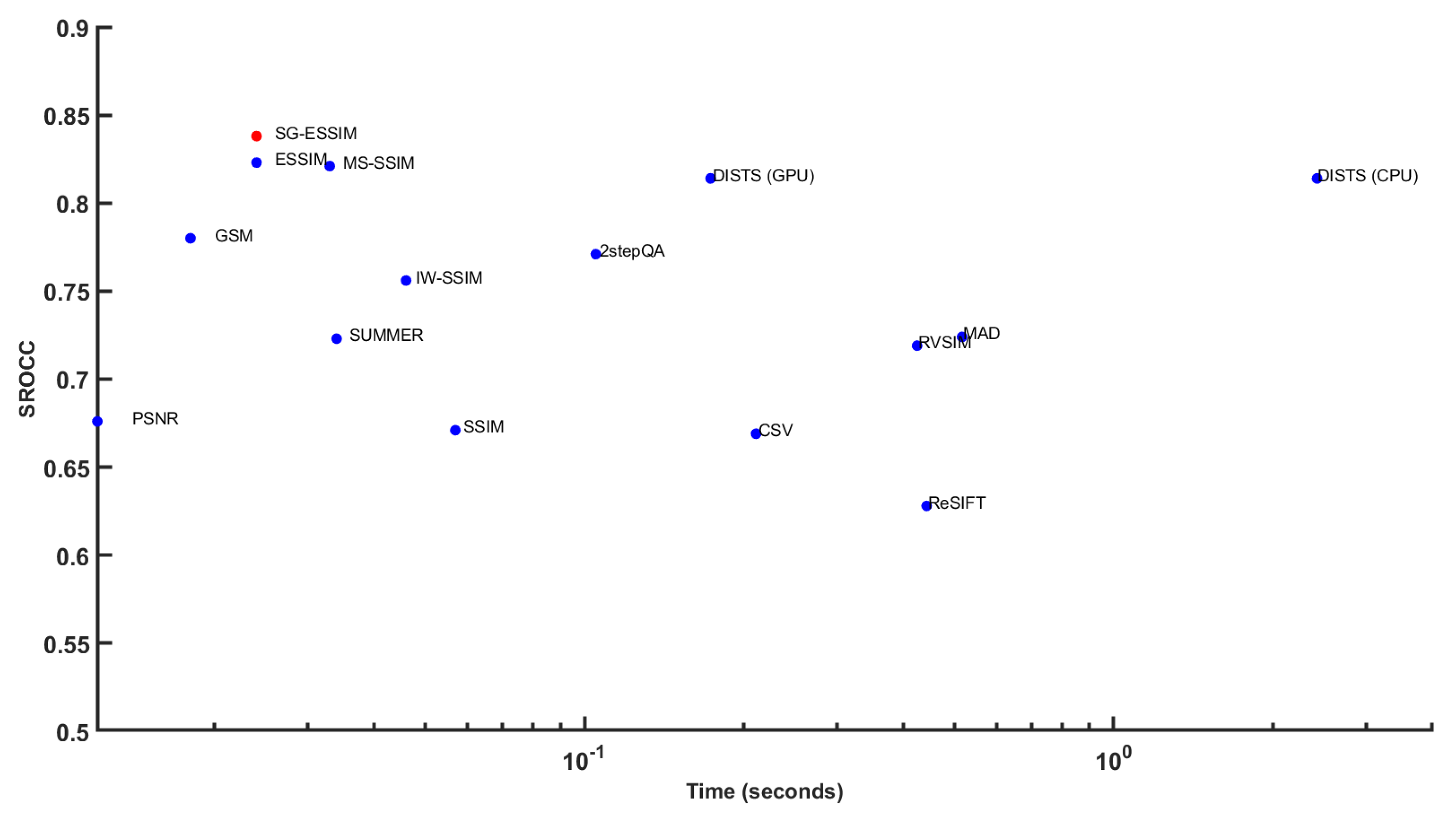
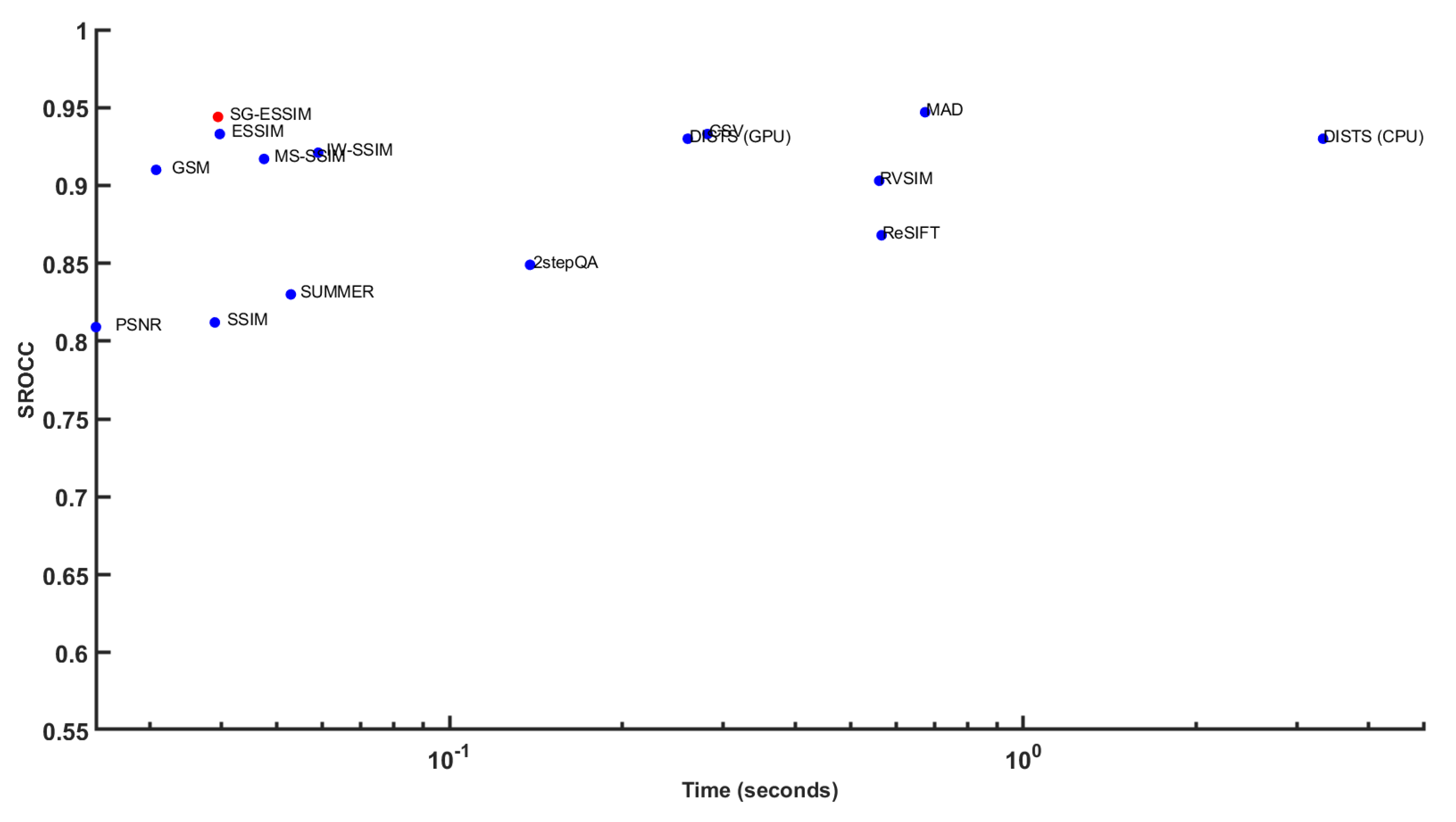
5. Experimental Results and Analysis
6. Conclusions
Funding
Institutional Review Board Statement
Informed Consent Statement
Data Availability Statement
Acknowledgments
Conflicts of Interest
Abbreviations
| AGN | additive Gaussian noise; |
| ANC | additive noise in color components; |
| CA | chromatic aberrations; |
| CC | contrast change; |
| CCS | change in color saturation; |
| CN | comfort noise; |
| CNN | convolutional neural network; |
| CPU | central processing unit; |
| DEN | image denoising; |
| FR-IQA | full-reference image quality assessment; |
| GB | Gaussian blur; |
| GPU | graphics processing unit; |
| HFN | high frequency noise; |
| HVS | human visual system; |
| ICQD | image color quantization with dither; |
| IN | impulse noise; |
| IQA | image quality assessment; |
| JGTE | JPEG transmission error; |
| JPEG | joint photographic experts group; |
| KROCC | Kendall’s rank order correlation coefficient; |
| LCNI | lossy compression of noisy images; |
| MGN | multiplicative Gaussian noise; |
| MN | masked noise; |
| MOS | mean opinion score; |
| MS | mean shift; |
| MSE | mean squared error; |
| NEPN | noneccentricity pattern noise; |
| NR-IQA | no-reference image quality assessment; |
| PLCC | Pearson’s linear correlation coefficient; |
| PSNR | peak signal-to-noise ratio; |
| QN | quantization noise; |
| RR-IQA | reduced-reference image quality assessment; |
| SCN | spatially correlated noise; |
| SG | saliency guided; |
| SROCC | Spearman’s rank order correlation coefficient; |
| SSR | space sampling and reconstruction |
References
- Ding, K.; Ma, K.; Wang, S.; Simoncelli, E.P. Comparison of full-reference image quality models for optimization of image processing systems. Int. J. Comput. Vis. 2021, 129, 1258–1281. [Google Scholar] [CrossRef]
- Chen, B.; Zhu, L.; Zhu, H.; Yang, W.; Lu, F.; Wang, S. The Loop Game: Quality Assessment and Optimization for Low-Light Image Enhancement. arXiv 2022, arXiv:2202.09738. [Google Scholar]
- Goyal, B.; Gupta, A.; Dogra, A.; Koundal, D. An adaptive bitonic filtering based edge fusion algorithm for Gaussian denoising. Int. J. Cogn. Comput. Eng. 2022, 3, 90–97. [Google Scholar] [CrossRef]
- Saito, Y.; Miyata, T. Recovering Texture with a Denoising-Process-Aware LMMSE Filter. Signals 2021, 2, 286–303. [Google Scholar] [CrossRef]
- Chubarau, A.; Akhavan, T.; Yoo, H.; Mantiuk, R.K.; Clark, J. Perceptual image quality assessment for various viewing conditions and display systems. Electron. Imaging 2020, 2020, 67-1. [Google Scholar] [CrossRef]
- Saupe, D.; Hahn, F.; Hosu, V.; Zingman, I.; Rana, M.; Li, S. Crowd workers proven useful: A comparative study of subjective video quality assessment. In Proceedings of the QoMEX 2016: 8th International Conference on Quality of Multimedia Experience, Lisbon, Portugal, 6–8 June 2016. [Google Scholar]
- Ponomarenko, N.; Ieremeiev, O.; Lukin, V.; Egiazarian, K.; Jin, L.; Astola, J.; Vozel, B.; Chehdi, K.; Carli, M.; Battisti, F.; et al. Color image database TID2013: Peculiarities and preliminary results. In Proceedings of the European Workshop on Visual Information Processing (EUVIP), Paris, France, 10–12 June 2013; pp. 106–111. [Google Scholar]
- Larson, E.C.; Chandler, D.M. Most apparent distortion: Full-reference image quality assessment and the role of strategy. J. Electron. Imaging 2010, 19, 011006. [Google Scholar]
- Zhai, G.; Min, X. Perceptual image quality assessment: A survey. Sci. China Inf. Sci. 2020, 63, 1–52. [Google Scholar] [CrossRef]
- Liu, H.; Heynderickx, I. Visual attention in objective image quality assessment: Based on eye-tracking data. IEEE Trans. Circuits Syst. Video Technol. 2011, 21, 971–982. [Google Scholar]
- Zhang, L.; Shen, Y.; Li, H. VSI: A visual saliency-induced index for perceptual image quality assessment. IEEE Trans. Image Process. 2014, 23, 4270–4281. [Google Scholar] [CrossRef] [Green Version]
- Zhang, W.; Borji, A.; Wang, Z.; Le Callet, P.; Liu, H. The application of visual saliency models in objective image quality assessment: A statistical evaluation. IEEE Trans. Neural Netw. Learn. Syst. 2015, 27, 1266–1278. [Google Scholar] [CrossRef] [Green Version]
- Ma, Q.; Zhang, L. Saliency-based image quality assessment criterion. In Proceedings of the International Conference on Intelligent Computing, Shanghai, China, 15–18 September 2008; pp. 1124–1133. [Google Scholar]
- Zhang, L.; Zhang, L.; Mou, X.; Zhang, D. FSIM: A feature similarity index for image quality assessment. IEEE Trans. Image Process. 2011, 20, 2378–2386. [Google Scholar] [CrossRef] [Green Version]
- Kovesi, P.; Robotics and Vision Research Group. Image features from phase congruency. Videre J. Comput. Vis. Res. 1999, 1, 1–26. [Google Scholar]
- Wang, Z.; Li, Q. Information content weighting for perceptual image quality assessment. IEEE Trans. Image Process. 2010, 20, 1185–1198. [Google Scholar] [CrossRef]
- Shi, C.; Lin, Y. Full reference image quality assessment based on visual salience with color appearance and gradient similarity. IEEE Access 2020, 8, 97310–97320. [Google Scholar] [CrossRef]
- Varga, D. Full-Reference Image Quality Assessment Based on Grünwald–Letnikov Derivative, Image Gradients, and Visual Saliency. Electronics 2022, 11, 559. [Google Scholar] [CrossRef]
- Zhang, X.; Feng, X.; Wang, W.; Xue, W. Edge strength similarity for image quality assessment. IEEE Signal Process. Lett. 2013, 20, 319–322. [Google Scholar] [CrossRef]
- Lin, H.; Hosu, V.; Saupe, D. KADID-10k: A large-scale artificially distorted IQA database. In Proceedings of the 2019 Eleventh International Conference on Quality of Multimedia Experience (QoMEX), Berlin, Germany, 5–7 June 2019; pp. 1–3. [Google Scholar]
- Ponomarenko, N.; Lukin, V.; Zelensky, A.; Egiazarian, K.; Carli, M.; Battisti, F. TID2008-a database for evaluation of full-reference visual quality assessment metrics. Adv. Mod. Radioelectron. 2009, 10, 30–45. [Google Scholar]
- Yang, X.; Sun, Q.; Wang, T. Image quality assessment via spatial structural analysis. Comput. Electr. Eng. 2018, 70, 349–365. [Google Scholar] [CrossRef]
- Wang, Z.; Bovik, A.C.; Sheikh, H.R.; Simoncelli, E.P. Image quality assessment: From error visibility to structural similarity. IEEE Trans. Image Process. 2004, 13, 600–612. [Google Scholar] [CrossRef] [Green Version]
- Brunet, D.; Vrscay, E.R.; Wang, Z. On the mathematical properties of the structural similarity index. IEEE Trans. Image Process. 2011, 21, 1488–1499. [Google Scholar] [CrossRef]
- Nilsson, J.; Akenine-Möller, T. Understanding ssim. arXiv 2020, arXiv:2006.13846. [Google Scholar]
- Wang, Z.; Simoncelli, E.P.; Bovik, A.C. Multiscale structural similarity for image quality assessment. In Proceedings of the Thrity-Seventh Asilomar Conference on Signals, Systems & Computers, 2003, Pacific Grove, CA, USA, 9–12 November 2003; Volume 2, pp. 1398–1402. [Google Scholar]
- Sampat, M.P.; Wang, Z.; Gupta, S.; Bovik, A.C.; Markey, M.K. Complex wavelet structural similarity: A new image similarity index. IEEE Trans. Image Process. 2009, 18, 2385–2401. [Google Scholar] [CrossRef]
- Chen, G.H.; Yang, C.L.; Po, L.M.; Xie, S.L. Edge-based structural similarity for image quality assessment. In Proceedings of the 2006 IEEE International Conference on Acoustics Speech and Signal Processing Proceedings, Toulouse, France, 14–19 May 2006; Volume 2, p. II. [Google Scholar]
- Liu, A.; Lin, W.; Narwaria, M. Image quality assessment based on gradient similarity. IEEE Trans. Image Process. 2011, 21, 1500–1512. [Google Scholar] [PubMed]
- Zhu, J.; Wang, N. Image quality assessment by visual gradient similarity. IEEE Trans. Image Process. 2011, 21, 919–933. [Google Scholar] [PubMed]
- Ma, J.; Wu, J.; Li, L.; Dong, W.; Xie, X.; Shi, G.; Lin, W. Blind image quality assessment with active inference. IEEE Trans. Image Process. 2021, 30, 3650–3663. [Google Scholar] [CrossRef]
- Chetouani, A.; Pedersen, M. Image Quality Assessment without Reference by Combining Deep Learning-Based Features and Viewing Distance. Appl. Sci. 2021, 11, 4661. [Google Scholar] [CrossRef]
- Vosta, S.; Yow, K.C. A CNN-RNN Combined Structure for Real-World Violence Detection in Surveillance Cameras. Appl. Sci. 2022, 12, 1021. [Google Scholar] [CrossRef]
- Amirshahi, S.A.; Pedersen, M.; Yu, S.X. Image quality assessment by comparing CNN features between images. J. Imaging Sci. Technol. 2016, 60, 60410-1. [Google Scholar] [CrossRef]
- Krizhevsky, A.; Sutskever, I.; Hinton, G.E. Imagenet classification with deep convolutional neural networks. Adv. Neural Inf. Process. Syst. 2012, 25, 1097–1105. [Google Scholar] [CrossRef]
- Barla, A.; Franceschi, E.; Odone, F.; Verri, A. Image kernels. In Proceedings of the International Workshop on Support Vector Machines, Niagara Falls, ON, Canada, 10 August 2002; pp. 83–96. [Google Scholar]
- Amirshahi, S.A.; Pedersen, M.; Beghdadi, A. Reviving traditional image quality metrics using CNNs. Color Imaging Conf. 2018, 26, 241–246. [Google Scholar] [CrossRef]
- Ahn, S.; Choi, Y.; Yoon, K. Deep learning-based distortion sensitivity prediction for full-reference image quality assessment. In Proceedings of the IEEE/CVF Conference on Computer Vision and Pattern Recognition, Nashville, TN, USA, 20–25 June 2021; pp. 344–353. [Google Scholar]
- Chubarau, A.; Clark, J. VTAMIQ: Transformers for Attention Modulated Image Quality Assessment. arXiv 2021, arXiv:2110.01655. [Google Scholar]
- Bosse, S.; Maniry, D.; Müller, K.R.; Wiegand, T.; Samek, W. Deep neural networks for no-reference and full-reference image quality assessment. IEEE Trans. Image Process. 2017, 27, 206–219. [Google Scholar] [CrossRef] [PubMed] [Green Version]
- Okarma, K. Combined full-reference image quality metric linearly correlated with subjective assessment. In Proceedings of the International Conference on Artificial Intelligence and Soft Computing, Zakopane, Poland, 13–17 June 2010; pp. 539–546. [Google Scholar]
- Okarma, K. Combined image similarity index. Opt. Rev. 2012, 19, 349–354. [Google Scholar] [CrossRef]
- Okarma, K. Extended hybrid image similarity–combined full-reference image quality metric linearly correlated with subjective scores. Elektron. Elektrotechnika 2013, 19, 129–132. [Google Scholar] [CrossRef] [Green Version]
- Oszust, M. Full-reference image quality assessment with linear combination of genetically selected quality measures. PLoS ONE 2016, 11, e0158333. [Google Scholar] [CrossRef] [PubMed] [Green Version]
- Lukin, V.V.; Ponomarenko, N.N.; Ieremeiev, O.I.; Egiazarian, K.O.; Astola, J. Combining full-reference image visual quality metrics by neural network. In Proceedings of the Human Vision and Electronic Imaging XX, SPIE, San Francisco, CA, USA, 9–12 February 2015; Volume 9394, pp. 172–183. [Google Scholar]
- Levkine, G. Prewitt, Sobel and Scharr gradient 5 × 5 convolution matrices. Image Process. Artic. Second. Draft. 2012, 1–17. [Google Scholar]
- Kim, D.J.; Lee, H.C.; Lee, T.S.; Lee, K.W.; Lee, B.H. Edge-Based Gaze Planning for Salient Proto-Objects. Appl. Mech. Mater. 2013, 330, 1003–1007. [Google Scholar] [CrossRef]
- Pedersen, M.; Hardeberg, J.Y. Full-reference image quality metrics: Classification and evaluation. Found. Trends® Comput. Graph. Vis. 2012, 7, 1–80. [Google Scholar]
- Sheikh, H.R.; Bovik, A.C.; De Veciana, G. An information fidelity criterion for image quality assessment using natural scene statistics. IEEE Trans. Image Process. 2005, 14, 2117–2128. [Google Scholar] [CrossRef] [Green Version]
- Yu, X.; Bampis, C.G.; Gupta, P.; Bovik, A.C. Predicting the quality of images compressed after distortion in two steps. IEEE Trans. Image Process. 2019, 28, 5757–5770. [Google Scholar] [CrossRef]
- Temel, D.; AlRegib, G. CSV: Image quality assessment based on color, structure, and visual system. Signal Process. Image Commun. 2016, 48, 92–103. [Google Scholar] [CrossRef] [Green Version]
- Ding, K.; Ma, K.; Wang, S.; Simoncelli, E.P. Image quality assessment: Unifying structure and texture similarity. arXiv 2020, arXiv:2004.07728. [Google Scholar] [CrossRef] [PubMed]
- Temel, D.; AlRegib, G. ReSIFT: Reliability-weighted sift-based image quality assessment. In Proceedings of the 2016 IEEE International Conference on Image Processing (ICIP), Phoenix, AZ, USA, 25–28 September 2016; pp. 2047–2051. [Google Scholar]
- Yang, G.; Li, D.; Lu, F.; Liao, Y.; Yang, W. RVSIM: A feature similarity method for full-reference image quality assessment. EURASIP J. Image Video Process. 2018, 2018, 1–15. [Google Scholar] [CrossRef] [Green Version]
- Temel, D.; AlRegib, G. Perceptual image quality assessment through spectral analysis of error representations. Signal Process. Image Commun. 2019, 70, 37–46. [Google Scholar] [CrossRef] [Green Version]

| Database | Ref. Images | Dist. Images | Dist. Types | Dist. Levels |
|---|---|---|---|---|
| KADID-10k [20] | 81 | 10,125 | 25 | 5 |
| TID2013 [7] | 25 | 3000 | 24 | 5 |
| TID2008 [21] | 25 | 1700 | 17 | 4 |
| CSIQ [8] | 30 | 866 | 6 | 4–5 |
| Computer model | STRIX Z270H Gaming |
| Operating system | Windows 10 |
| Memory | 15 GB |
| CPU | Intel(R) Core(TM) i7-7700K CPU 4.20 GHz (8 cores) |
| GPU | Nvidia GeForce GTX 1080 |
| KADID-10k [20] | TID2013 [7] | |||||
|---|---|---|---|---|---|---|
| FR-IQA Metric | PLCC | SROCC | KROCC | PLCC | SROCC | KROCC |
| 2stepQA [50] | 0.768 | 0.771 | 0.571 | 0.736 | 0.733 | 0.550 |
| CSV [51] | 0.671 | 0.669 | 0.531 | 0.852 | 0.848 | 0.657 |
| DISTS [52] | 0.809 | 0.814 | 0.626 | 0.759 | 0.711 | 0.524 |
| ESSIM [19] | 0.644 | 0.823 | 0.634 | 0.740 | 0.797 | 0.627 |
| GSM [29] | 0.780 | 0.780 | 0.588 | 0.789 | 0.787 | 0.593 |
| IW-SSIM [16] | 0.781 | 0.756 | 0.524 | 0.832 | 0.778 | 0.598 |
| MAD [8] | 0.716 | 0.724 | 0.535 | 0.827 | 0.778 | 0.600 |
| MS-SSIM [26] | 0.819 | 0.821 | 0.630 | 0.794 | 0.785 | 0.604 |
| PSNR | 0.479 | 0.676 | 0.488 | 0.616 | 0.646 | 0.467 |
| ReSIFT [53] | 0.648 | 0.628 | 0.468 | 0.630 | 0.623 | 0.471 |
| RVSIM [54] | 0.728 | 0.719 | 0.540 | 0.763 | 0.683 | 0.520 |
| SSIM [23] | 0.670 | 0.671 | 0.489 | 0.618 | 0.616 | 0.437 |
| SUMMER [55] | 0.719 | 0.723 | 0.540 | 0.623 | 0.622 | 0.472 |
| SG-ESSIM | 0.739 | 0.838 | 0.650 | 0.878 | 0.805 | 0.636 |
| TID2008 [21] | CSIQ [8] | |||||
|---|---|---|---|---|---|---|
| FR-IQA Metric | PLCC | SROCC | KROCC | PLCC | SROCC | KROCC |
| 2stepQA [50] | 0.757 | 0.769 | 0.574 | 0.841 | 0.849 | 0.655 |
| CSV [51] | 0.852 | 0.851 | 0.659 | 0.933 | 0.933 | 0.766 |
| DISTS [52] | 0.705 | 0.668 | 0.488 | 0.930 | 0.930 | 0.764 |
| ESSIM [19] | 0.658 | 0.876 | 0.696 | 0.814 | 0.933 | 0.768 |
| GSM [29] | 0.782 | 0.781 | 0.578 | 0.906 | 0.910 | 0.729 |
| IW-SSIM [16] | 0.842 | 0.856 | 0.664 | 0.804 | 0.921 | 0.753 |
| MAD [8] | 0.831 | 0.829 | 0.639 | 0.950 | 0.947 | 0.796 |
| MS-SSIM [26] | 0.838 | 0.846 | 0.648 | 0.913 | 0.917 | 0.743 |
| PSNR | 0.447 | 0.489 | 0.346 | 0.853 | 0.809 | 0.599 |
| ReSIFT [53] | 0.627 | 0.632 | 0.484 | 0.884 | 0.868 | 0.695 |
| RVSIM [54] | 0.789 | 0.743 | 0.566 | 0.923 | 0.903 | 0.728 |
| SSIM [23] | 0.669 | 0.675 | 0.485 | 0.812 | 0.812 | 0.606 |
| SUMMER [55] | 0.817 | 0.823 | 0.623 | 0.826 | 0.830 | 0.658 |
| SG-ESSIM | 0.853 | 0.888 | 0.708 | 0.836 | 0.944 | 0.786 |
| Direct Average | Weighted Average | |||||
|---|---|---|---|---|---|---|
| FR-IQA Metric | PLCC | SROCC | KROCC | PLCC | SROCC | KROCC |
| 2stepQA [50] | 0.776 | 0.781 | 0.587 | 0.765 | 0.768 | 0.572 |
| CSV [51] | 0.827 | 0.825 | 0.653 | 0.740 | 0.738 | 0.582 |
| DISTS [52] | 0.801 | 0.781 | 0.601 | 0.795 | 0.785 | 0.599 |
| ESSIM [19] | 0.714 | 0.857 | 0.681 | 0.673 | 0.830 | 0.647 |
| GSM [29] | 0.814 | 0.815 | 0.622 | 0.789 | 0.789 | 0.596 |
| IW-SSIM [16] | 0.815 | 0.828 | 0.635 | 0.800 | 0.780 | 0.570 |
| MAD [8] | 0.831 | 0.820 | 0.643 | 0.763 | 0.758 | 0.573 |
| MS-SSIM [26] | 0.841 | 0.842 | 0.656 | 0.821 | 0.822 | 0.633 |
| PSNR | 0.599 | 0.655 | 0.475 | 0.520 | 0.660 | 0.470 |
| ReSIFT [53] | 0.697 | 0.688 | 0.530 | 0.655 | 0.641 | 0.483 |
| RVSIM [54] | 0.801 | 0.762 | 0.589 | 0.752 | 0.725 | 0.549 |
| SSIM [23] | 0.692 | 0.694 | 0.504 | 0.668 | 0.669 | 0.485 |
| SUMMER [55] | 0.746 | 0.750 | 0.573 | 0.720 | 0.720 | 0.540 |
| SG-ESSIM | 0.827 | 0.869 | 0.695 | 0.783 | 0.843 | 0.661 |
| 2stepQA [50] | CSV [51] | DISTS [52] | ESSIM [19] | GSM [29] | MAD [8] | MS-SSIM [26] | ReSIFT [53] | RVSIM [54] | SSIM [23] | SG-ESSIM | |
|---|---|---|---|---|---|---|---|---|---|---|---|
| AGN | 0.817 | 0.938 | 0.845 | 0.911 | 0.899 | 0.912 | 0.624 | 0.831 | 0.886 | 0.848 | 0.936 |
| ANC | 0.590 | 0.862 | 0.786 | 0.806 | 0.823 | 0.800 | 0.387 | 0.749 | 0.836 | 0.779 | 0.855 |
| SCN | 0.860 | 0.939 | 0.859 | 0.938 | 0.927 | 0.929 | 0.683 | 0.839 | 0.868 | 0.851 | 0.935 |
| MN | 0.395 | 0.748 | 0.814 | 0.711 | 0.704 | 0.658 | 0.372 | 0.702 | 0.734 | 0.775 | 0.715 |
| HFN | 0.828 | 0.927 | 0.868 | 0.890 | 0.884 | 0.902 | 0.704 | 0.869 | 0.895 | 0.889 | 0.920 |
| IN | 0.715 | 0.848 | 0.674 | 0.825 | 0.813 | 0.743 | 0.766 | 0.824 | 0.865 | 0.810 | 0.833 |
| QN | 0.886 | 0.892 | 0.810 | 0.904 | 0.911 | 0.895 | 0.720 | 0.745 | 0.869 | 0.817 | 0.911 |
| GB | 0.853 | 0.933 | 0.926 | 0.970 | 0.954 | 0.915 | 0.762 | 0.937 | 0.970 | 0.910 | 0.969 |
| DEN | 0.900 | 0.952 | 0.899 | 0.956 | 0.955 | 0.922 | 0.819 | 0.907 | 0.926 | 0.876 | 0.963 |
| JPEG | 0.867 | 0.944 | 0.897 | 0.923 | 0.933 | 0.924 | 0.784 | 0.905 | 0.930 | 0.893 | 0.950 |
| JP2K | 0.891 | 0.966 | 0.931 | 0.946 | 0.934 | 0.929 | 0.790 | 0.928 | 0.946 | 0.806 | 0.949 |
| JGTE | 0.806 | 0.800 | 0.906 | 0.826 | 0.866 | 0.768 | 0.582 | 0.712 | 0.831 | 0.701 | 0.823 |
| J2TE | 0.854 | 0.887 | 0.865 | 0.902 | 0.893 | 0.854 | 0.742 | 0.835 | 0.882 | 0.813 | 0.899 |
| NEPN | 0.775 | 0.811 | 0.833 | 0.799 | 0.804 | 0.803 | 0.792 | 0.693 | 0.771 | 0.634 | 0.801 |
| BLOCK | 0.044 | 0.183 | 0.302 | 0.649 | 0.588 | −0.322 | 0.382 | 0.440 | 0.545 | 0.564 | 0.623 |
| MS | 0.660 | 0.654 | 0.752 | 0.712 | 0.728 | 0.708 | 0.732 | 0.418 | 0.559 | 0.738 | 0.706 |
| CC | 0.430 | 0.227 | 0.464 | 0.453 | 0.466 | 0.420 | 0.027 | −0.055 | 0.132 | 0.355 | 0.452 |
| CCS | −0.258 | 0.809 | 0.789 | −0.297 | 0.676 | −0.059 | −0.055 | −0.209 | 0.366 | 0.742 | 0.010 |
| MGN | 0.747 | 0.884 | 0.790 | 0.853 | 0.831 | 0.888 | 0.653 | 0.765 | 0.853 | 0.804 | 0.900 |
| CN | 0.858 | 0.924 | 0.907 | 0.910 | 0.902 | 0.904 | 0.596 | 0.882 | 0.914 | 0.797 | 0.916 |
| LCNI | 0.902 | 0.965 | 0.932 | 0.957 | 0.945 | 0.950 | 0.713 | 0.897 | 0.933 | 0.877 | 0.952 |
| ICQD | 0.808 | 0.919 | 0.832 | 0.904 | 0.901 | 0.867 | 0.739 | 0.770 | 0.871 | 0.820 | 0.928 |
| CA | 0.702 | 0.845 | 0.879 | 0.839 | 0.835 | 0.760 | 0.568 | 0.838 | 0.871 | 0.740 | 0.835 |
| SSR | 0.926 | 0.976 | 0.944 | 0.965 | 0.961 | 0.949 | 0.801 | 0.944 | 0.956 | 0.822 | 0.964 |
| All | 0.733 | 0.848 | 0.711 | 0.797 | 0.787 | 0.778 | 0.785 | 0.623 | 0.683 | 0.616 | 0.805 |
| 2stepQA [50] | CSV [51] | DISTS [52] | ESSIM [19] | GSM [29] | MAD [8] | MS-SSIM [26] | ReSIFT [53] | RVSIM [54] | SSIM [23] | SG-ESSIM | |
|---|---|---|---|---|---|---|---|---|---|---|---|
| AGN | 0.766 | 0.922 | 0.812 | 0.875 | 0.855 | 0.872 | 0.610 | 0.771 | 0.840 | 0.805 | 0.913 |
| ANC | 0.627 | 0.893 | 0.811 | 0.792 | 0.821 | 0.803 | 0.354 | 0.762 | 0.829 | 0.780 | 0.900 |
| SCN | 0.814 | 0.932 | 0.838 | 0.909 | 0.904 | 0.901 | 0.727 | 0.810 | 0.837 | 0.800 | 0.920 |
| MN | 0.450 | 0.781 | 0.830 | 0.744 | 0.736 | 0.673 | 0.304 | 0.728 | 0.760 | 0.797 | 0.825 |
| HFN | 0.818 | 0.936 | 0.870 | 0.899 | 0.889 | 0.894 | 0.749 | 0.881 | 0.886 | 0.871 | 0.921 |
| IN | 0.659 | 0.819 | 0.626 | 0.777 | 0.764 | 0.650 | 0.767 | 0.777 | 0.836 | 0.776 | 0.786 |
| QN | 0.850 | 0.894 | 0.770 | 0.884 | 0.903 | 0.851 | 0.708 | 0.730 | 0.836 | 0.784 | 0.873 |
| GB | 0.877 | 0.923 | 0.909 | 0.966 | 0.948 | 0.896 | 0.759 | 0.904 | 0.963 | 0.866 | 0.964 |
| DEN | 0.919 | 0.970 | 0.931 | 0.974 | 0.971 | 0.928 | 0.786 | 0.923 | 0.939 | 0.873 | 0.963 |
| JPEG | 0.895 | 0.948 | 0.894 | 0.938 | 0.937 | 0.931 | 0.774 | 0.914 | 0.926 | 0.880 | 0.959 |
| JP2K | 0.910 | 0.984 | 0.953 | 0.966 | 0.949 | 0.941 | 0.837 | 0.935 | 0.970 | 0.745 | 0.972 |
| JGTE | 0.851 | 0.790 | 0.907 | 0.859 | 0.871 | 0.781 | 0.606 | 0.735 | 0.860 | 0.666 | 0.855 |
| J2TE | 0.845 | 0.852 | 0.833 | 0.875 | 0.880 | 0.802 | 0.742 | 0.778 | 0.854 | 0.769 | 0.863 |
| NEPN | 0.803 | 0.752 | 0.882 | 0.742 | 0.784 | 0.801 | 0.749 | 0.761 | 0.732 | 0.588 | 0.729 |
| Block | 0.441 | 0.770 | 0.618 | 0.876 | 0.843 | −0.362 | 0.765 | 0.743 | 0.782 | 0.804 | 0.905 |
| MS | 0.655 | 0.594 | 0.681 | 0.611 | 0.638 | 0.563 | 0.711 | 0.322 | 0.525 | 0.629 | 0.683 |
| CC | 0.597 | 0.330 | 0.649 | 0.624 | 0.634 | 0.548 | 0.042 | −0.018 | 0.194 | 0.502 | 0.642 |
| All | 0.769 | 0.851 | 0.668 | 0.876 | 0.781 | 0.829 | 0.846 | 0.632 | 0.743 | 0.675 | 0.888 |
| 2stepQA [50] | CSV [51] | DISTS [52] | ESSIM [19] | GSM [29] | MAD [8] | MS-SSIM [26] | ReSIFT [53] | RVSIM [54] | SSIM [23] | SG-ESSIM | |
|---|---|---|---|---|---|---|---|---|---|---|---|
| Level 1 | 0.246 | 0.424 | 0.235 | 0.388 | 0.372 | 0.388 | 0.166 | 0.181 | 0.248 | 0.204 | 0.448 |
| Level 2 | 0.394 | 0.626 | 0.440 | 0.547 | 0.512 | 0.368 | 0.049 | 0.401 | 0.430 | 0.276 | 0.569 |
| Level 3 | 0.539 | 0.635 | 0.367 | 0.638 | 0.523 | 0.442 | 0.240 | 0.415 | 0.416 | 0.084 | 0.660 |
| Level 4 | 0.571 | 0.749 | 0.606 | 0.766 | 0.669 | 0.284 | 0.172 | 0.699 | 0.702 | 0.208 | 0.787 |
| Level 5 | 0.663 | 0.787 | 0.664 | 0.875 | 0.745 | 0.308 | 0.397 | 0.788 | 0.803 | 0.202 | 0.861 |
| All | 0.733 | 0.848 | 0.711 | 0.797 | 0.787 | 0.778 | 0.785 | 0.623 | 0.683 | 0.616 | 0.805 |
| 2stepQA [50] | CSV [51] | DISTS [52] | ESSIM [19] | GSM [29] | MAD [8] | MS-SSIM [26] | ReSIFT [53] | RVSIM [54] | SSIM [23] | SG-ESSIM | |
|---|---|---|---|---|---|---|---|---|---|---|---|
| Level 1 | 0.470 | 0.638 | 0.566 | 0.655 | 0.639 | 0.432 | 0.067 | 0.457 | 0.634 | 0.368 | 0.691 |
| Level 2 | 0.619 | 0.683 | 0.381 | 0.773 | 0.636 | 0.520 | 0.221 | 0.437 | 0.513 | 0.105 | 0.807 |
| Level 3 | 0.573 | 0.774 | 0.581 | 0.826 | 0.677 | 0.239 | 0.059 | 0.707 | 0.761 | 0.190 | 0.849 |
| Level 4 | 0.610 | 0.829 | 0.628 | 0.905 | 0.718 | 0.232 | 0.275 | 0.788 | 0.825 | 0.241 | 0.891 |
| All | 0.769 | 0.851 | 0.668 | 0.876 | 0.781 | 0.829 | 0.846 | 0.632 | 0.743 | 0.675 | 0.888 |
Publisher’s Note: MDPI stays neutral with regard to jurisdictional claims in published maps and institutional affiliations. |
© 2022 by the author. Licensee MDPI, Basel, Switzerland. This article is an open access article distributed under the terms and conditions of the Creative Commons Attribution (CC BY) license (https://creativecommons.org/licenses/by/4.0/).
Share and Cite
Varga, D. Saliency-Guided Local Full-Reference Image Quality Assessment. Signals 2022, 3, 483-496. https://doi.org/10.3390/signals3030028
Varga D. Saliency-Guided Local Full-Reference Image Quality Assessment. Signals. 2022; 3(3):483-496. https://doi.org/10.3390/signals3030028
Chicago/Turabian StyleVarga, Domonkos. 2022. "Saliency-Guided Local Full-Reference Image Quality Assessment" Signals 3, no. 3: 483-496. https://doi.org/10.3390/signals3030028
APA StyleVarga, D. (2022). Saliency-Guided Local Full-Reference Image Quality Assessment. Signals, 3(3), 483-496. https://doi.org/10.3390/signals3030028