1. Introduction
With the fast development of communication networks, such as 5G and WiFi networks, millimeter waves have emerged as a key technology to achieve high data rate transmission. With the increase in frequency, the perception ability of wireless signal improves. In the future, wireless signals will not only have communication ability but also have sensing ability, such as millimeter waves in 5G and Terahertz in 6G. Compared with the traditional communication technologies, millimeter waves have the capability of sensing. Hence, wireless sensing based on millimeter waves has attracted more research attention. Human activity recognition is widely investigated in the field of ubiquitous sensing based on inertial sensors, computer vision, or LiDAR. Compared with those traditional approaches, human activity recognition based on millimeter-wave radar has many unique advantages. Firstly, compared with LiDAR, millimeter-wave radar has a better penetration ability of floating particles such as smoke and dust. This advantage means that the process of activity recognition of millimeter-wave radar has strong environmental adaptability. Secondly, because the millimeter-wave radar uses radio frequency signals, it will not return the privacy screen of the target person, which means that the radar monitoring will not reveal personal identity information. This edge enables indoor activity recognition based on the millimeter-wave radar more widely applicable, such as nursing homes, kindergartens, wards, etc.
In previous studies, researchers generally used collected data such as point cloud, range–Doppler, and echo intensity from millimeter-wave radar echo signals for activity recognition. For instance, RadHAR [
1] shows how to voxelize sparse and non-uniform point clouds and feed them into a classifier. Additionally, in [
2], since the single-sensor system can only observe the radial component of the micro-Doppler signal, researchers propose a multi-static sensor consisting of two bistatic micro-Doppler sensors to enhance the classification of micro-Doppler signatures to improve activity recognition accuracy. In [
3], also using Doppler information, the researchers propose an environmental impact mitigation method by analyzing millimeter-wave signals in a Doppler–range domain. In terms of extracting activity features, deep learning is favored by researchers [
4], among which convolutional neural networks (CNN) and long short-term memory networks (LSTM) are widely used. Because most human actions have time-series characteristics, these two network models are often combined. For example, some researchers [
5] adopt LSTM + CNN network to classify activities.
However, most of these studies only focus on a single type of data that cannot comprehensively depict the activity feature. The approaches based on point clouds merely leverage the distributions of point clouds in 3D space but do not consider the moving speed. In contrast, the methods using range–Doppler does not take the distributions of point clouds into consideration. Our goal is to design a multi-model network by fusing multiple types of input data to increase the recognition accuracy based on mmWave. We are going to extract the features from the two kinds of data, fuse them, and then classify the activities. Therefore, in this work, we propose a new method for activity recognition that uses both 3D point cloud data and range–Doppler data as input. We summarize the main contributions in this work as follows.
First, we propose a multi-model deep learning model to fuse the point cloud and range–Doppler to achieve activity recognition based on millimeter-wave radar. We voxelize and merge the 3D point cloud data in multiple frames into a 4D array. We further merge and convert the range–Doppler data in the same number of frames into a 3D array. Afterward, we use two sub-networks to train these two kinds of data separately. The 3D CNN + LSTM network is applied for the point cloud data, while the 3D CNN network is used for the range–Doppler data. Next, we fuse the outputs of the two networks, that is, the activity features contained in each kind of data, to obtain a more comprehensive activity feature than utilizing only one kind of data. Finally, the fused features are input into the fully connected layer for classification.
Second, we use the IWR1843 device of Texas Instruments to collect data on six activities, i.e., boxing, jumping, squatting, walking, circling, and high-knee lifting, and construct a dataset for activity recognition.
Finally, experimental results show that the classification using the fused features of these two kinds of data is about 1% more accurate than merely using point cloud or range–Doppler, which shows that the use of multiple types of information has a positive effect on the recognition accuracy.
The paper is organized as follows.
Section 2 is related work.
Section 3 is the preliminary of millimeter-wave radar that introduces the working principle.
Section 4 introduces the pre-processing of data and different network structures.
Section 5 expounds on the process of the experiment and analyzes the experiment results.
Section 6 gives the conclusion of this paper.
2. Related Work
Research on classification and identification using millimeter-wave radar has been increasing in recent years. Many researchers use millimeter-wave radar to identify human gait [
6,
7], gestures [
8,
9], and activities [
10,
11,
12,
13,
14,
15,
16]. They extract different types of data from the raw data returned by the radar and use machine learning [
17] and deep learning to extract the features of the target to achieve the purpose of classification and identification. For example, in [
7], researchers collect a large variety of human walking data with millimeter-wave radar and use this data set to evaluate the performance of some deep learning networks. In [
8], the researchers discuss the feasibility of AI-assisted gesture recognition using 802.11 ad 60 GHz (millimeter wave) technology in smartphones. They design a CNN + LSTM sequence model and a tiny pure CNN model to recognize different gestures, including hands and fingers, with high precision and small size.
In the experiments of recognizing human activities, the experimenters use a variety of methods. For example, in [
10], the experimenters converted the obtained point cloud data into micro-Doppler features and used CNN to extract the features to classify actions. In [
11], the researchers proposed a new point network. They collect human echo signals through radar, extract the range–velocity sequence, and then add the time dimension on the basis of two-dimensional data to form the range–velocity–time data. Compared with directly processing the original point cloud, the point network can learn the structural features from the micromotion trajectory more effectively; that is, it can learn the dynamic motion better. In [
12], the researchers find that measurements with very high azimuth and elevation resolution can locate scatterers from the human body. The authors extract features from the point cloud using deep recurrent neural networks with two-dimensional convolutional networks (DRNN). Some researchers are dissatisfied with using a single type of feature for identification but use multiple data as input. In [
13], the researchers extracted the time–range, time–Doppler, and range–Doppler features of the radar signal and fused them, and then used CNN for learning and classification and obtained a higher accuracy than the traditional two-dimensional recognition method. Some researchers try to improve the speed of human action recognition. In [
14], the researchers propose a field-programmable gate array (FPGA) based convolutional neural network (CNN) acceleration method. They use the spectrogram of the millimeter-wave radar echo as the CNN input and finally find that the method not only maintains a high classification accuracy but also improves the execution speed. Some researchers have built a system framework for higher accuracy. In [
15], the researchers propose a hands-free human activity recognition framework leveraging millimeter-wave sensors. They implement the network in one architecture and optimize it to have higher accuracy than those networks that can only obtain a single result (i.e., only pose estimation or activity recognition). Some researchers focus on solving some application problems in the real world. For example, in [
16], researchers tried to solve these two problems: poor recognition accuracy in noisy environments and being unable to provide a real-time response due to long time delay. They propose m-activity, a method that can reduce the noise caused by the environmental multipath effect and run smoothly while realizing har. The off-line accuracy and implementation accuracy of this method are verified in the gym, and good results are obtained.
3. Preliminary of Millimeter Radar
The carrier wavelength of millimeter-wave radar is electromagnetic waves in the range of 1–10 mm, which has the characteristics of a short wavelength, a wide frequency band, and it is not easy for it to interfere. Millimeter-wave radar was used in the military in the early days, and in recent years, with the development of technology, it has been gradually used in automotive electronics, drones, and other fields. At present, the frequency bands of millimeter-wave radars are mainly divided into three categories: 24 GHz frequency band, 77 GHz frequency band, and 76–81 GHz frequency band. The radar used in this paper works at 76–81 GHz. The biggest feature of this frequency band is the wide bandwidth, so it has a high range resolution and is suitable for distinguishing different actions of the human body.
Due to its high resolution, low signal processing complexity, and low cost, FMCW is the most used modulation method for millimeter-wave radar. FMCW radar system mainly includes transceiver antenna, RF front-end, modulation signal, a signal processing module, etc. Millimeter-wave radar can detect the distance, azimuth, and relative speed of the target through the correlation processing of the received signal and the transmitted signal. The principle of ranging and speed measurement of FMCW radar is introduced below.
3.1. The Principle of Ranging of FMCW Radar
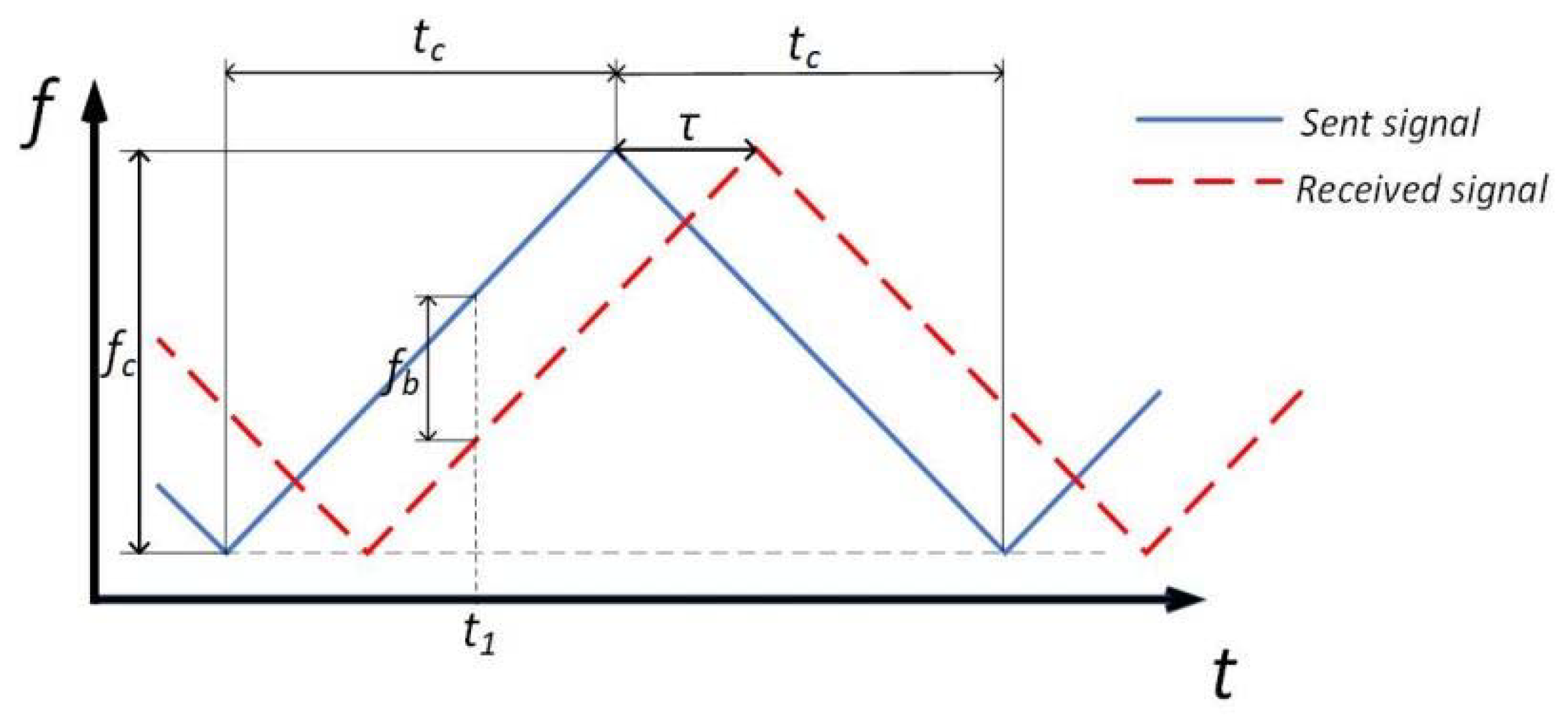
FMCW radar transmits continuous waves with frequency changes in the frequency scanning period. There is a certain frequency difference between the echo reflected by the object and the transmitted signal. The distance information between the target and the radar can be obtained by measuring the frequency difference.
Let
,
be the frequency variation functions of sending and receiving signals, respectively, and
be the initial frequency. Assuming that the relative speed
is zero. The relationship on the rising edge of the signal is as follows:
There is a beat frequency function:
Hence, we can draw the
Figure 1 below, where
is half of the frequency sweeping cycle,
is the frequency sweeping bandwidth, and
is the time from signal transmission to reception.
Because of
, from the geometric relationship
in
Figure 1, it can be concluded that:
where
is the speed of light.
To sum up, the detection range of the FMCW radar is determined by Equation (4), and the key parameter is the frequency difference between transmission and reception, which directly affects the selection of ADC sampling rate. Although the scanning bandwidth also has an impact on the detection distance, it does not affect the selection of ADC when it is a fixed value.
3.2. The Principle of Speed Measurement of FMCW Radar
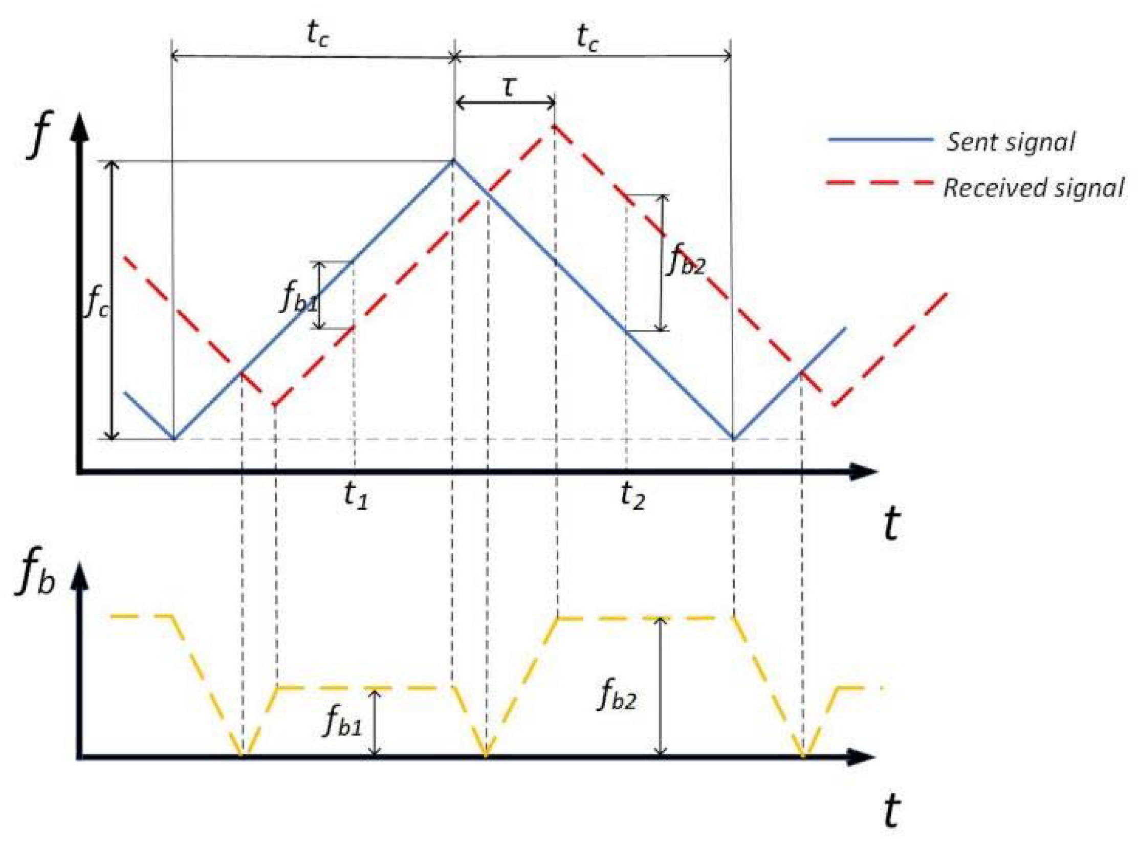
If there is no Doppler frequency, the frequency difference during the rising edge is equal to the measured value during the falling edge. For moving targets, the frequency difference during the rising or falling edge is different. We can measure the distance and speed through these two frequency differences. Therefore, we can draw the curve of the beat frequency versus time, as shown in
Figure 2, where
refers to beat frequency.
From the Doppler effect, we know:
is the central frequency of the transmitted signal, and from Equation (4), we can obtain:
Substituting Equations (5)–(7) into Equation (8) yields Equations (9) and (10):
Subtracting Equation (9) from Equation (10), then we can obtain the formula of the relative speed
(11):
Thus, FMCW radar can realize ranging and speed measurement.
4. Activity Recognition Based on Fusion of Point Cloud and Range–Doppler
4.1. Data Pre-Processing
In the actual data acquisition process, the signal will be disturbed by noise due to the influence of the environment, hardware, and other factors. Therefore, denoising is needed in data pre-processing. There are many signal denoising methods, such as CFAR (Constant False-Alarm Rate) algorithm, Fourier transforms, wavelet transforms [
18], compressed sensing [
19,
20,
21], and so on. They have different advantages and are applied in different scenarios. Here we use CA-CFAR (Cell Average Constant False-Alarm Rate) algorithm. CFAR refers to the technology where the radar system judges the signal and noise output by the receiver to determine whether the target signal exists under the condition of keeping the false alarm rate constant. CFAR detector first processes the input noise and then determines a threshold, which is compared with the input signal. If the input signal exceeds this threshold, it is judged as having a target; otherwise, it is judged as having no target. CA-CFAR algorithm is one of the most classical mean CFAR algorithms. It uses the average value of a certain range of cells around the current data to be detected to determine the threshold of the tested cell. It has the lowest loss rate of all CFAR algorithms.
Since the millimeter-wave radar has a wide coverage area, and the distance between the collected person and the radar is relatively fixed, we consider removing some unnecessary data. This is performed to prevent excessive invalid data, which reduce the speed and accuracy of recognition. Hence, we filter the data whose range values are between 1 m and 2 m. In the following part, we explain how to pre-process 3D point cloud data and range–Doppler data, respectively.
Considering the irregularity of the number of 3D point cloud data in each frame, we must convert it into a data format with a fixed size and shape so that it can be effectively input into a convolutional neural network (CNN). Therefore, we first establish a three-dimensional discrete coordinate system. Then use Equations (12)–(14) for each frame to calculate the scale of the
x,
y, and
z axes, in which the two ends of the coordinate axis are the minimum and maximum value of the point cloud data of the axis. Then we create a 10 × 32 × 32 array and fill the point cloud coordinates of each frame into the corresponding position of the array. It is worth mentioning that we do not directly fill in the coordinate value but count the number of points located in each array. This is to avoid having two different coordinates filled in the same position. Thus, we achieve a three-dimensional array of size 10 × 32 × 32 that represents the distribution of the point cloud in this frame. However, when the sampling rate is eight frames per second, a single frame of data cannot reflect the timing characteristics between frames. Therefore, we developed a fourth dimension based on the three-dimensional data, which represents the time series, and merged the eight frames of data to obtain a 4D array with a size of 8 × 10 × 32 × 32. So far, the pre-processing of 3D point cloud data is over.
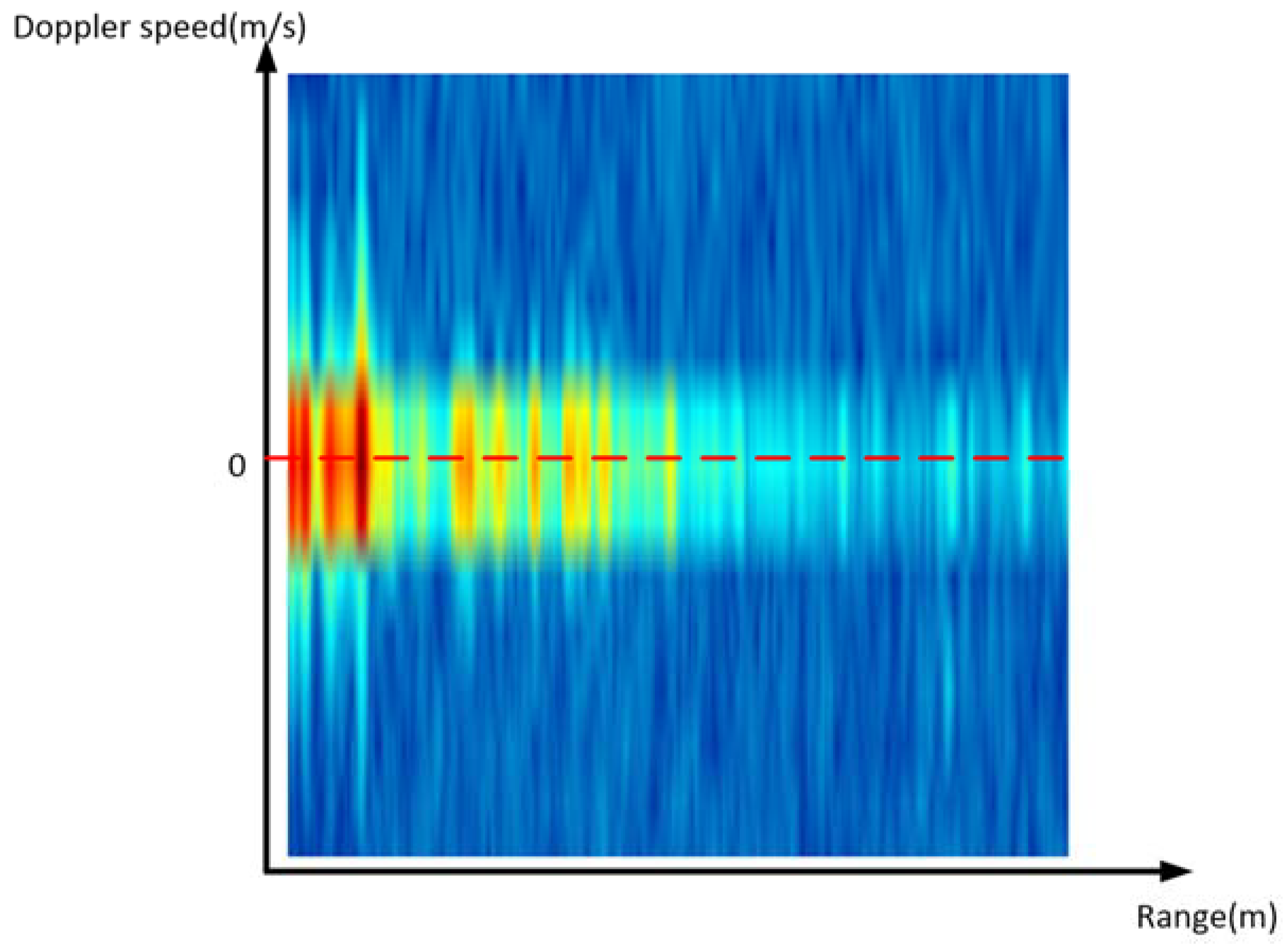
On the other hand, the pre-processing of range–Doppler data is relatively simple. As is shown in
Figure 3, the range–Doppler data are presented in a picture-like form. Its abscissa is the range, the ordinate is the Doppler speed, and the value in the picture is the thermal value. Hence, we export the range–Doppler data from each frame separately and achieve a 2D array of size 32 × 32. Then, to synchronize with the 3D point cloud, we merge the range–Doppler data in eight frames and finally achieve a 3D array with a size of 8 × 32 × 32.
4.2. Using Only 3D Point Cloud Data as Input
We know that 3D point cloud data reflects the spatial and temporal characteristics of actions. For the extraction of spatial features, we use three-dimensional CNN, and for time series features, a simple CNN network may not be able to respond well to the time series connection between frames, so we designed two kinds of networks for comparative experiments. The first network uses only CNN, while the second network adds an LSTM layer after the CNN.
4.2.1. Three-Dimensional Convolutional Neural Network (3D CNN)
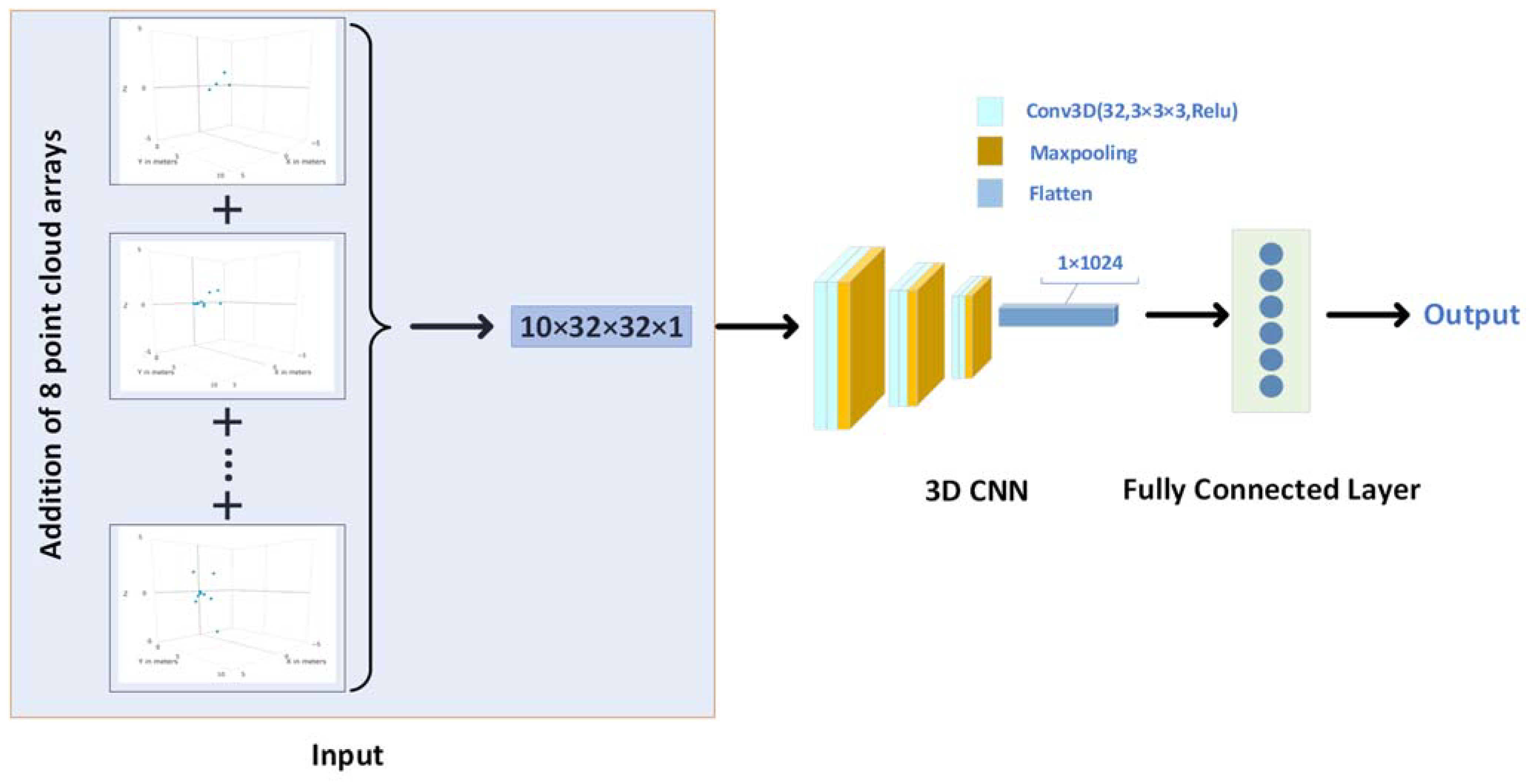
For 3D point cloud data, we first consider that it reflects the spatial features of actions, and in the data pre-processing part above, we also voxelize each frame of data into a fixed size 3D array, so it is not difficult to think that we can use 3D CNN to extract the spatial features. However, considering the sparsity of point clouds (the number of point clouds in a frame is generally less than 10), we merge the point cloud from eight frames into one frame, that is, add eight consecutive three-dimensional arrays bit by bit to achieve a new three-dimensional array with a size of 10 × 32 × 32, which is denser. Then it is used as the input of the convolution network to train the network.
The structure of the network is shown in
Figure 4. In the convolution part, we use the ‘Conv3D-Conv3D-Maxpooling’ structure three times. The 3D convolution layers all use the convolution kernel of (3, 3, 3), the number of convolution kernels is 32, the padding is set to ‘same’, the activation function is Relu, and the stride is set to (1, 1, 1). The pool size of the maxpooling layer is set to (2, 2, 2), the stride is set to (1, 1, 1), and the padding is set to ‘valid’. Then the extracted features are flattened and input into the fully connected layer.
4.2.2. Three-Dimensional Convolutional Neural Network and Long Short-Term Memory Network (3D CNN + LSTM)
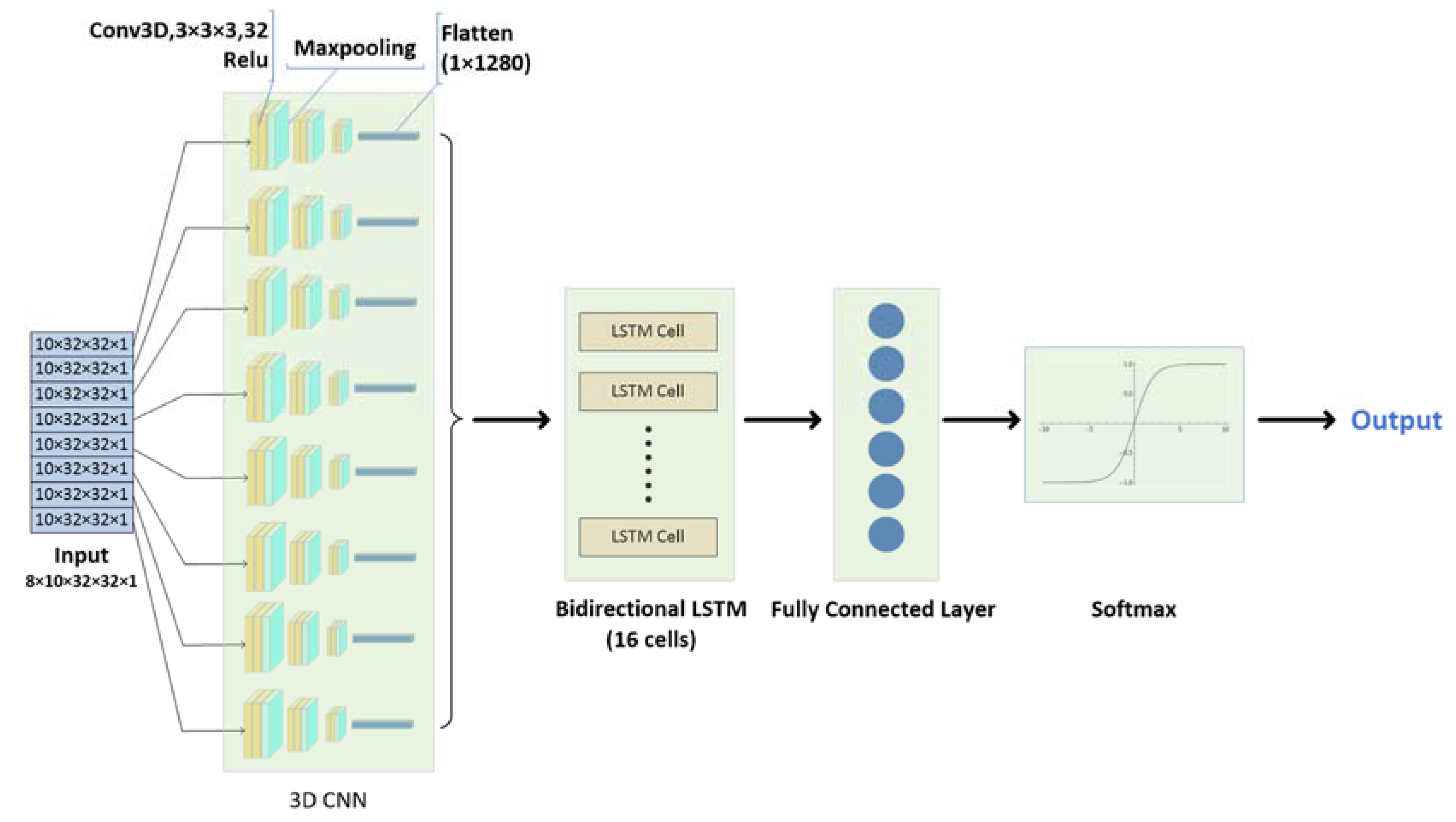
Considering that the activities are continuous, there is a timing characteristic between the received frames. Hence, we use a 3D CNN + LSTM network for training and classification. Because the acquisition rate is eight frames per second, and the duration of each activity is about one second, we pre-process the 3D point cloud data into a four-dimensional array of size 8 × 10 × 32 × 32, which includes the merging of 3D point cloud data received in one second. Because the input of LSTM must contain the parameter timesteps, we use the ‘TimeDistributed’ layer wrapper to encapsulate the convolutional layer, pooling layer, and flatten layer, adding a time dimension to the input data. As mentioned above, we set the value on this dimension to 8.
The structure of the network is shown in
Figure 5. In the convolution part, we use the ‘Conv3D-Conv3D-Maxpooling’ structure three times. The parameter settings are the same as in the first network. Then the extracted features are flattened and input into the bidirectional LSTM layer, whose number of hidden layer units is 16. Finally, a fully connected layer is used for classification after regularization, whose activation function is Softmax.
4.3. Using Only Range–Doppler Data as Input
In terms of data validity, it is not difficult to find that both 3D point cloud data and range–Doppler data are theoretically valid. Both types of data contain activity features that can be extracted by deep learning. Hence, we design two different networks and try to train them on range–Doppler data in order to compare the results with networks using other kinds of data as input. The two networks are: a three-dimensional convolutional neural network (3D CNN) and a two-dimensional convolutional neural network (2D CNN). The two networks are described below.
4.3.1. Three-Dimensional Convolutional Neural Network (3D CNN)
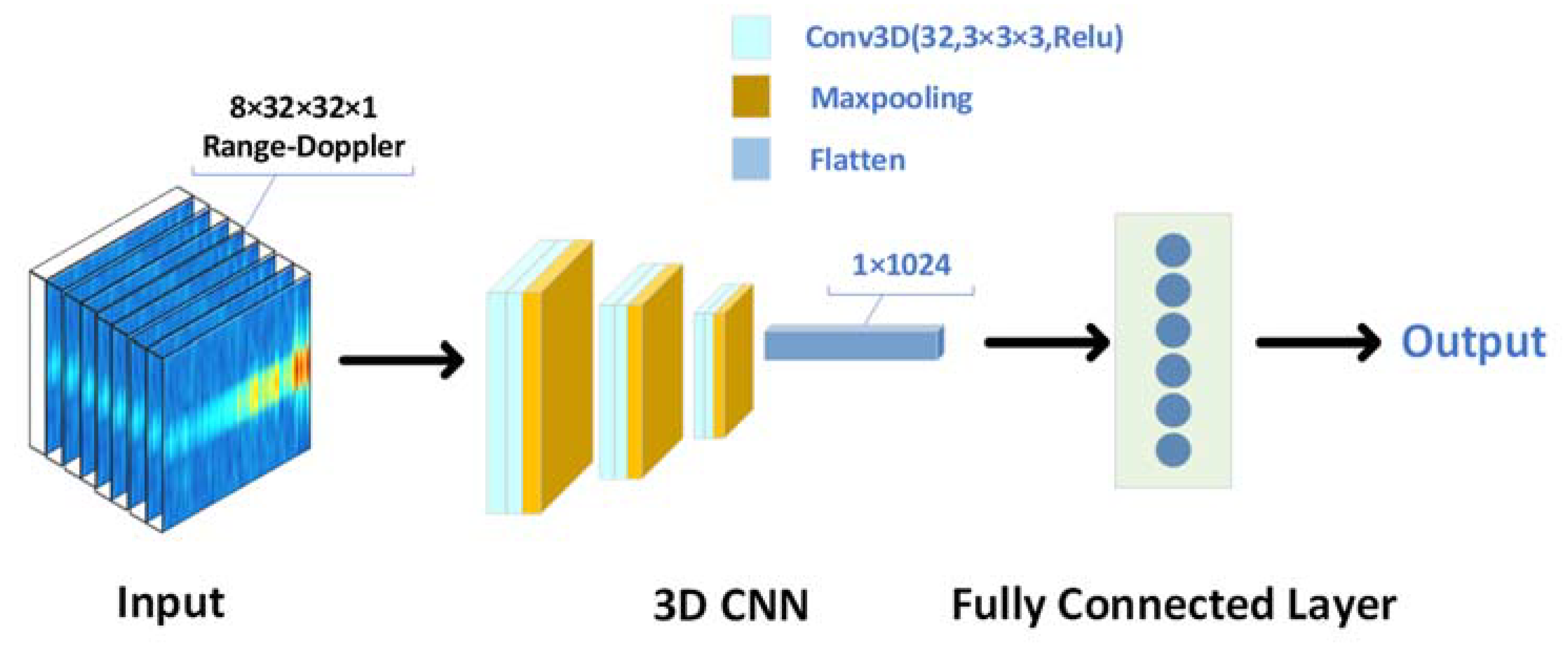
Because a piece of range–Doppler data is actually a superposition of multiple images in the time dimension, we try to use a 3D CNN to train the range–Doppler data. The structure of the network is shown in
Figure 6. As we can see, this network is similar to the convolutional part of the point cloud network. We used the structure of ‘Conv3D-Conv3D-Maxpooling’ three times, where the parameter settings are consistent with the network in Part B, without the ‘TimeDistributed’ layer wrapper encapsulating the layers. Then we input the features to the flattened layer and the fully connected layer for classification successively. The network takes eight frames of range–Doppler data as a set of input data, that is, the data with the shape of 8 × 32 × 32 × 1 can be regarded as a three-dimensional single channel stereo image, so the network can be understood as a classification network of three-dimensional images. However, different from the ordinary image classification network, the input data has not only spatial characteristics but also temporal characteristics. The temporal characteristics can be understood as the series between frames, that is, the characteristics reflected by Doppler velocity. This network can better learn the characteristics of dynamic actions rather than only extracting static two-dimensional features.
4.3.2. Two-Dimensional Convolutional Neural Network (2D CNN)
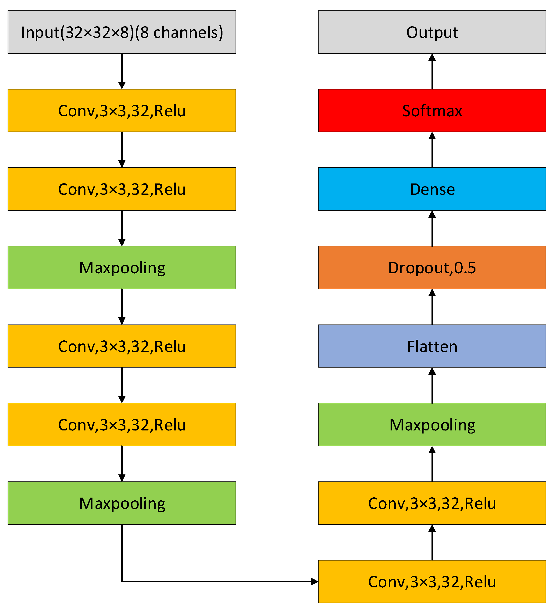
Since the duration of each activity is not strictly one second, it can be problematic to treat eight frames of range–Doppler data as a full representation of activity. Thus, instead of using 3D single-channel data as input, we consider designing a network that uses 2D multi-channel data as input. The structure of the network is shown in
Figure 7. It is worth noting that, different from 3D CNN, the convolutional layers change from three-dimensional to two-dimensional, and in the first convolutional layer, we set the input data shape to (32, 32, 8)—two-dimensional data with eight channels, width and height being 32. In order to make a valid comparison with the results of other networks, other parts of the network remain unchanged except for changing the shape of the input data. Therefore, we use the ‘Conv2D-Conv2D-Maxpooling’ structure three times and keep the parameters, such as the number and size of the convolution kernel, step size, etc., unchanged but only delete the depth dimension. Similarly, we input the features obtained by convolution into the flattened layer and the fully connected layer for classification.
4.4. Using Both 3D Point Cloud Data and Range–Doppler Data as Input
We know that the more types of information describing an object, the higher the classification accuracy and loss will be. Multimodal fusion is based on this principle [
22]. In our study, there are various kinds of information describing an activity, such as point cloud information, echo intensity information, range–Doppler information, and so on. This information describes the activity from different aspects, and the information contains different characteristics of the activity. If we extract these features and fuse them effectively, we can achieve more comprehensive features than using one kind of information alone. Therefore, we propose to fuse the features contained in the 3D point cloud information and the range–Doppler information. Of course, fusing more kinds of features will achieve a more comprehensive description of the activity, but the difficulty of their fusion will also increase accordingly, so this paper only fuses the features of point cloud information and range–Doppler information.
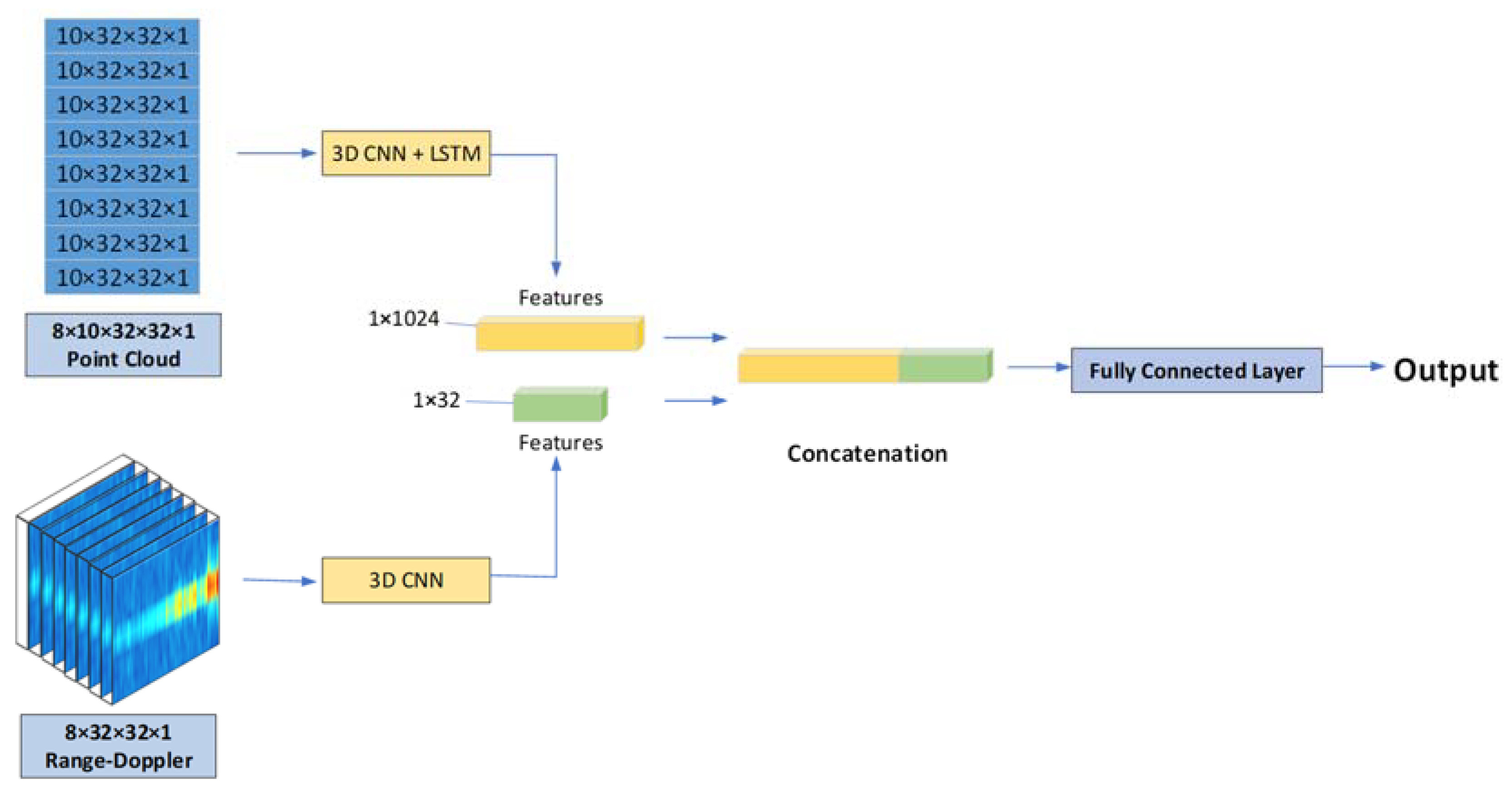
Taking the second network of part B and the first network of part C as an example, the network structure is shown in
Figure 8. We parallelize the networks of parts B and C and input the 3D point cloud data and range–Doppler data into these two networks, respectively. The input of the fully connected layers of the two networks is the features contained in the two kinds of information, so we output the results of the previous layer of the fully connected layer separately and found that they are all two-dimensional, and the first dimension is the amount of data. Hence, we feed these two features into the concatenate layer, merge them in the second dimension, and achieve a feature that contains two different features. Finally, we regularize this feature and feed it into a fully connected layer for classification.
5. Experiment and Results
5.1. Data Collecting and Experiment Setup
We adopt IWR1843, which is produced by Texas Instruments (TI), for data collecting. The IWR1843 device is an integrated single-chip millimeter-wave sensor based on FMCW radar technology, which can operate in the 76 GHz to 81 GHz band. IWR1843 includes three transmitting antennas and four receiving antennas, ADC converters, and a DSP subsystem [
23].
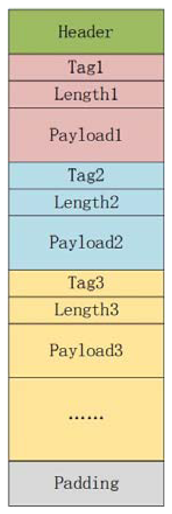
Data sent by the radar to the serial port is the hexadecimal data that has been processed by the above modules. The frame structure of the radar output is shown in
Figure 9. Each packet consists of the header, the TLV (Type, Length, Value) items, and the padding. Users can set different Type values to different output types of data. We achieve the data by setting the Type values corresponding to the 3D point cloud data and the range–Doppler data. Before collecting, we have configured the radar parameters, and some important parameters are shown in
Table 1.
After configuring, we connect the IWR1843 device to the computer and place it on a platform with a height of 1.2 m. The side where the antenna array is located faces the person doing the activity. In the process of data collection, the fixation of the millimeter-wave radar must be guaranteed. We design six activities, which are boxing in place, jumping in place, squatting, walking in place, circling in place, and high-knee lifting. Each activity is completed by 17 collectors and repeated for 20 s per person. During the data collection process, we decode the hexadecimal 3D point cloud data and range–Doppler data contained in the signal received by the serial port in real-time. After using one-hot encoding to label the data, we set the ratio of the amount of training data to the amount of validation data to be 4:1; that is, the training set accounts for 80% of the total data, while the verification set accounts for 20%. In order to control the variables to effectively compare the performance of the networks, we use the same set of data for training. In our experiments, we use a GPU server with a GTX3080 to train five kinds of networks.
5.2. Evaluation and Analysis
In order to train the model, the parameters are set as follows. First, we choose cross-entropy as the loss function. This loss function applies when the labels are multi-class patterns. Then we choose Adam as the optimizer. It uses the first-order moment estimation and second-order moment estimation of the gradient to dynamically adjust the learning rate of each parameter. The advantage is that each iteration of the learning rate has a clear range, which makes the parameter change very smooth. Accuracy is selected as the metrics method. Batch_size is set to 20.
Five kinds of networks are trained below. We first train the two networks of only inputting point cloud data and the two networks of only inputting range–Doppler data mentioned above, and then pick out the networks with the highest accuracy and the smallest loss, and then connect them in parallel. Then we input both point cloud data and range–Doppler data into the new network for training.
5.2.1. Using Only 3D Point Cloud Data as Input
As mentioned above in the data pre-processing section, we input the acquired 3D point cloud data into the two networks in two different data formats and then train them by 100 epochs separately. After training, we plot the validation set accuracy and loss downloaded from Tensorboard into
Figure 10 and
Figure 11 and find their maximum and minimum values, respectively, as shown in
Table 2.
According to the above curves and tables, adding the LSTM network to the pure convolution network improves the accuracy of the network, reduces the loss, and improves the convergence speed. This verifies that the point cloud data has obvious timing characteristics between frames. To better evaluate the precision, we visualize the confusion matrix, as shown in
Figure 12. Each column of the confusion matrix represents the predicted category, and the total number of each column represents the number of the data predicted as that category. While each row represents the true ascribed category of the data, the total number of the data for each row represents the number of data instances of that category. We find that the prediction difficulty of these activities, except circling, which is slightly more difficult, is all close.
5.2.2. Using Only Range–Doppler Data as Input
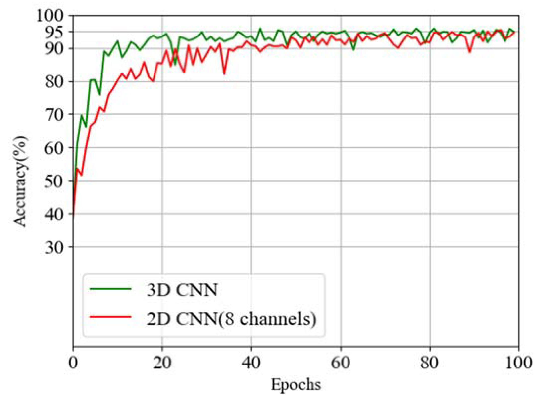
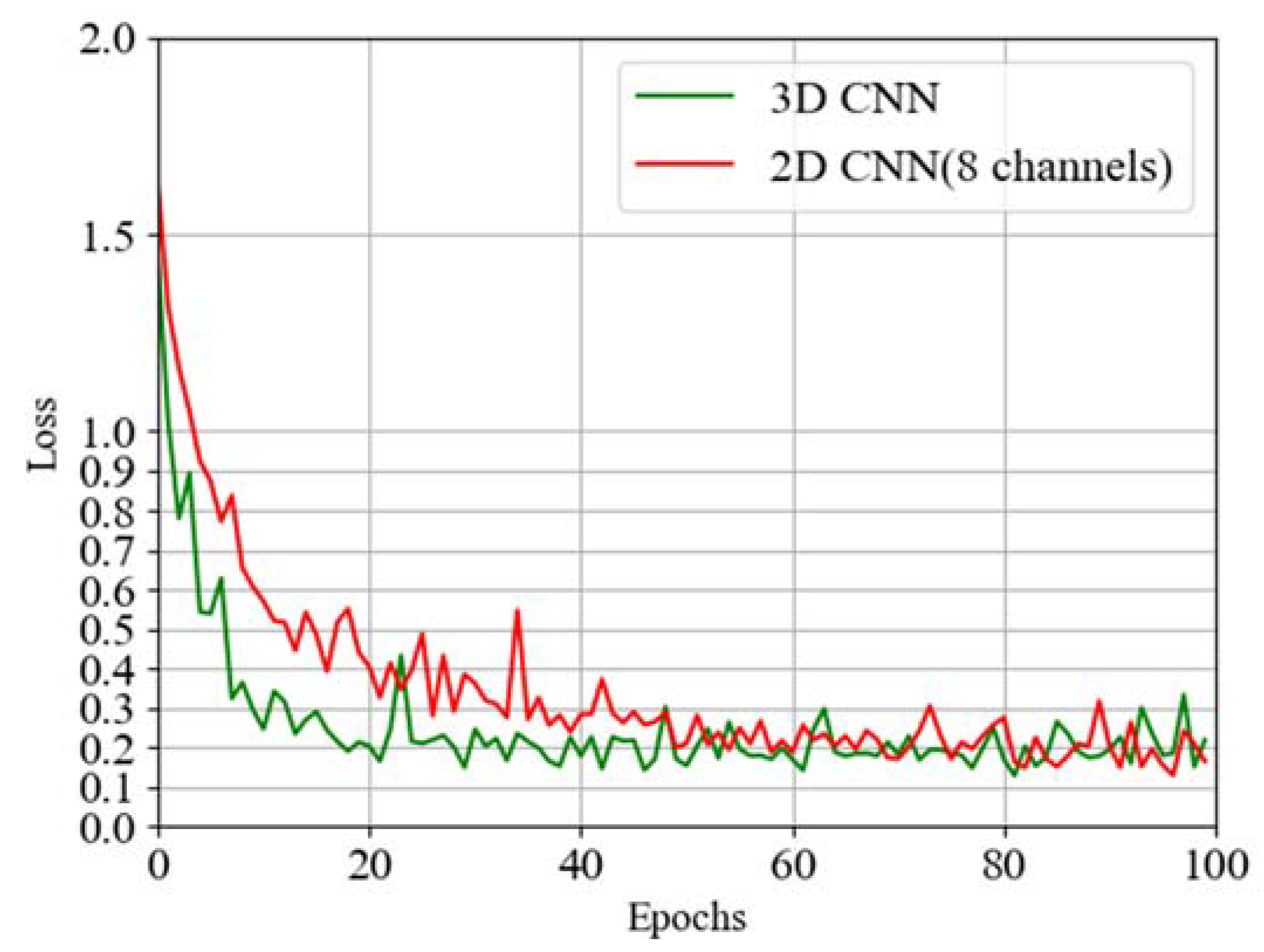
Similar to 3D point cloud data, we combine eight frames of range–Doppler data. For consolidation, we use two methods, i.e., adding a new dimension to keep the number of channels unchanged and increasing the number of channels while keeping the dimension unchanged. As mentioned above, different networks are used due to different data formats. The former uses a three-dimensional single-channel convolution network, while the latter uses a two-dimensional multi-channel convolution network. Their network structures are similar. After training the two networks with 100 epochs, respectively, we draw the curves of verification accuracy and loss into
Figure 13 and
Figure 14, find out the maximum value of accuracy and the minimum value of loss, respectively, and make
Table 3.
As can be seen from the above figures and table, 3D CNN has a slight advantage over 2D CNN in terms of accuracy and loss, with an accuracy of 0.42% higher and a loss of 0.005 lower. Moreover, by observing the two curves, we find that 3D CNN has obvious advantages in convergence speed, which also means that 3D CNN needs fewer hardware resources on the basis of training the same amount of data. By printing the model structures of the two networks, we find that the parameters of 3D CNN that need to be trained are far less than those of 2D CNN. The 3D CNN needs to train 131,622 parameters, while 2D CNN needs to train 279,076 parameters, which is more than twice as few as the latter. In order to compare the verification accuracy of each action in the 3D CNN network, we draw the confusion matrix, as shown in
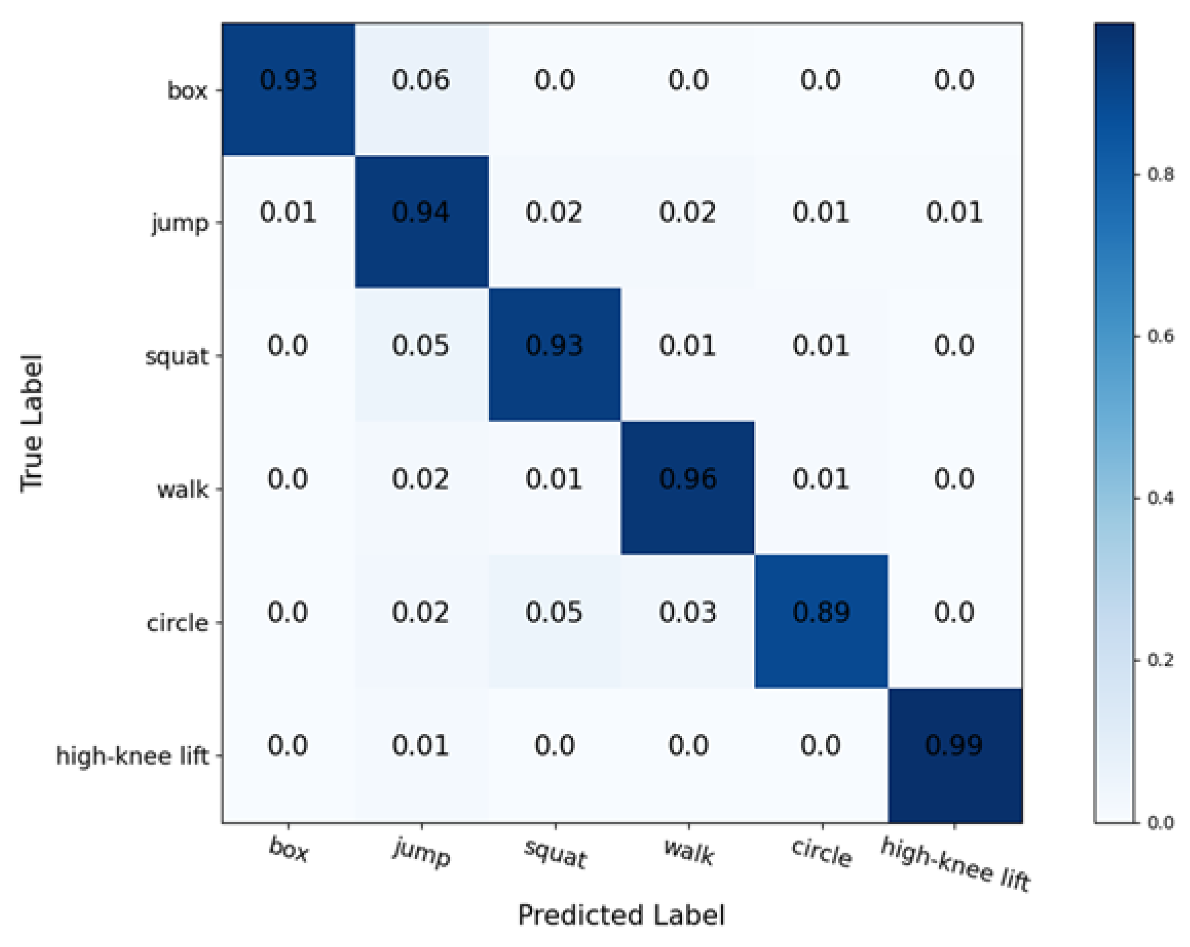
Figure 15. In this network, we find that high-knee lifting is easy to predict while circling is relatively difficult to identify. The spectrograms of other activities are similar.
5.2.3. Using Both 3D Point Cloud Data and Range–Doppler Data as Input
It can be concluded that, for point cloud data, the 3D CNN + LSTM has the highest accuracy and the lowest loss among the two networks, while for range–Doppler data, the 3D CNN performs best. Therefore, we choose these two networks to be the two parallel branches of the feature fusion network mentioned above. The obtained network structure is shown in
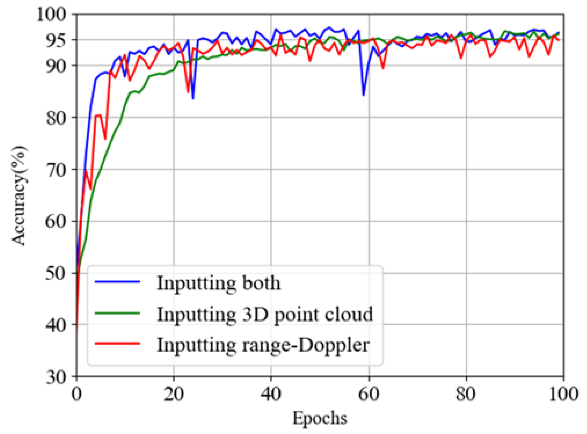
Figure 8. Hence, we train this network and draw the accuracy and loss images with the results of these three different networks in
Figure 16 and
Figure 17 after obtaining the results and tabulating the specific values, as shown in
Table 4.
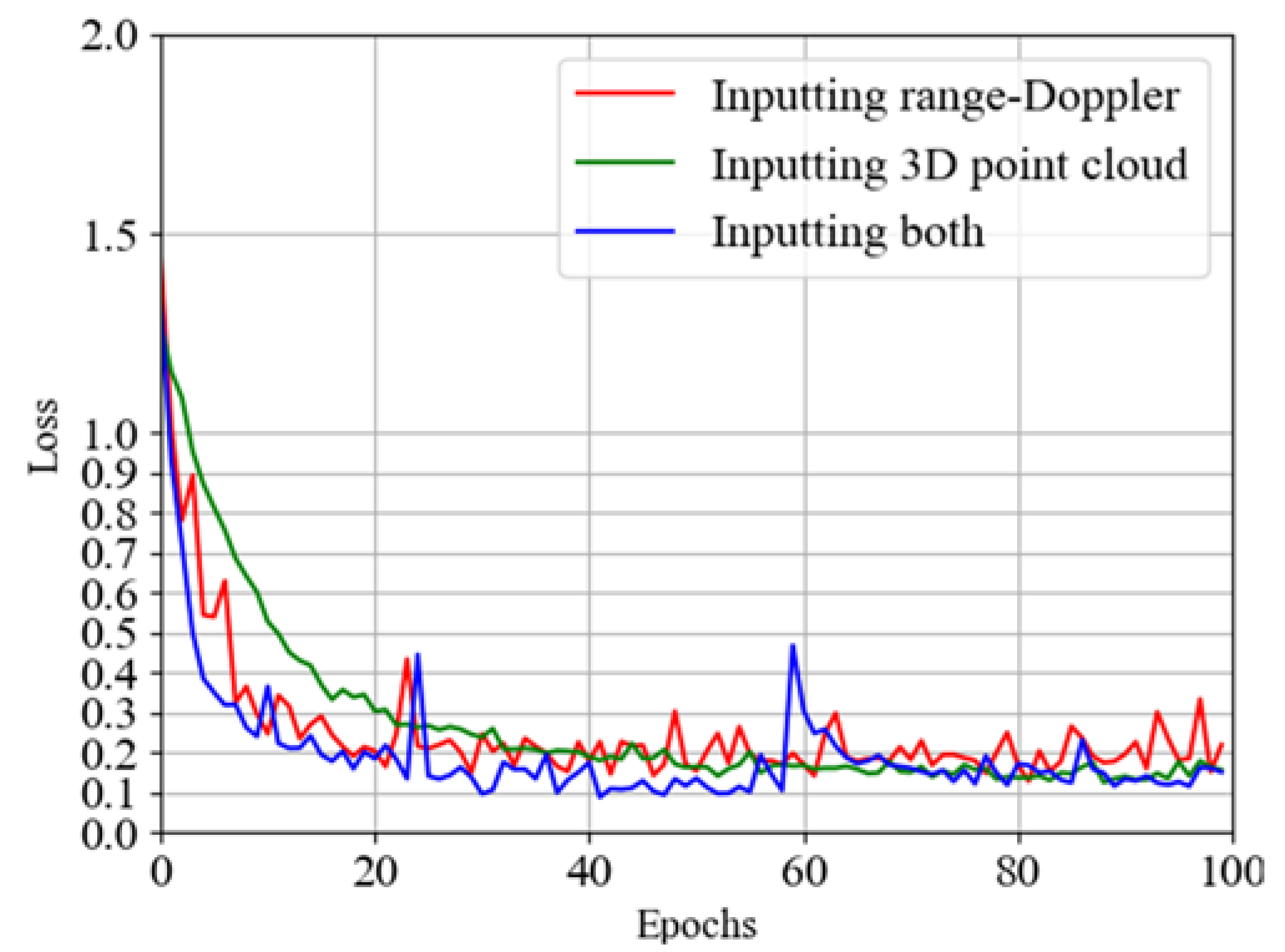
From the above results, we find that the network using both 3D point cloud data and range–Doppler data as input has better accuracy and loss than using one of them alone. This shows that using more kinds of data can extract more action features, which has a positive factor for the improvement of network performance. We also find that the convergence speed of the fusion network is faster. Similar to the above two networks, we also draw the confusion matrix, as shown in
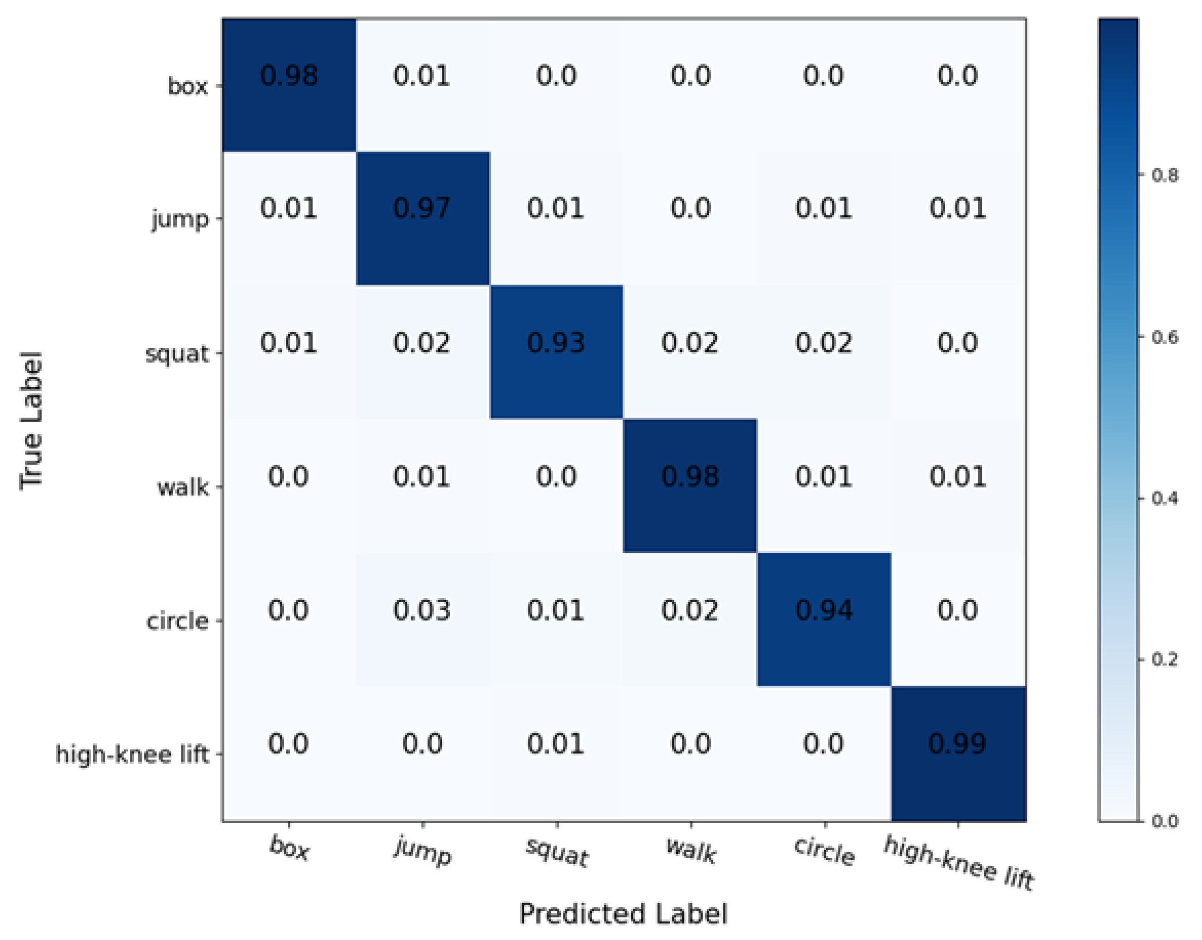
Figure 18, so as to analyze the verification accuracy of each action. We find that the prediction difficulty of these activities is all close except squatting and circling, which are slightly more difficult to identify.
The above experimental results tell us that the fusion network has better classification results. We further study this fusion network and carry out an ablation analysis. We change the depth of the network and then observe the changes in accuracy and loss value. We change the depth of the network by changing the number of repetitions of the structure of “Convolution Layer-Convolution Layer-Maxpooling Layer”. The purpose of this is not to change the overall structure of the network as much as possible so as to achieve the effect of controlling other variables. Based on the original network, we double and halve the repetition times of the structure of “Convolution Layer-Convolution Layer-Maxpooling Layer” in the two branch networks of the fusion network-3D point cloud branch network and range–Doppler branch network, respectively. In this way, we have obtained two new networks, one of which has 20 layers of 3D point cloud branch network and 18 layers of range–Doppler branch network, while the other has 11 layers of 3D point cloud branch network and 9 layers of range–Doppler branch network. The 3D point cloud branch network of the original network has 14 layers, while the range–Doppler branch network has 12 layers. We train and verify the two new networks with the same data, respectively, and draw the obtained accuracy and loss value into a table, as shown in
Table 5.
The above experimental results show that increasing or decreasing the number of network layers will lead to a decrease in accuracy and an increase in loss value, which means that the best number of network layers is the number of layers of the original network. We know that, generally speaking, when the parameters are adjusted reasonably, the more layers and neurons, the higher the accuracy, which explains why the network performance will deteriorate after reducing the number of layers. However, this is in contradiction with the phenomenon that the network performance still deteriorates after increasing the number of network layers. The reason is that the increasing number of network layers leads to overfitting.
6. Conclusions
Nowadays, with the deepening of the interconnection of all things, people pay more attention to millimeter-wave radar, which can ensure privacy and performance at the same time. In this paper, depth learning is used to classify people’s different actions collected by millimeter-wave radar. Different from previous studies, we increase the types of input data, input 3D point cloud data, and range–Doppler data into the network for training at the same time and then fuse the extracted features, respectively. Finally, the network performs better and achieves a recognition accuracy of 97.26%, which is about 1% higher than other networks with only one kind of data as input. This represents the success of our attempt to increase data types to achieve higher accuracy. We also consider that we can continue to expand data types, optimize the process of feature extraction, and better integrate different types of data in order to obtain better network performance, which requires further study.
Author Contributions
Conceptualization, Y.H. and W.L.; methodology, Y.H. and W.L.; software, Z.D.; validation, Y.H., W.L., Z.D., W.Z. and A.Z.; formal analysis, Y.H.; investigation, Y.H. and W.L.; resources, Y.H.; data curation, Y.H., W.L.; writing—original draft preparation, Y.H.; writing—review and editing, Y.H., W.L. and Z.L.; visualization, Z.D., W.Z. and A.Z.; supervision, Z.L.; project administration, Z.L.; funding acquisition, Z.L. All authors have read and agreed to the published version of the manuscript.
Funding
This work is supported by the National Natural Science Foundation of China (62171197) and Technology Development Program of Jilin Province (20210508059RQ and 20200201287JC).
Institutional Review Board Statement
Not applicable.
Informed Consent Statement
Not applicable.
Data Availability Statement
Not applicable.
Acknowledgments
In the process of research, we attained the help of Qinzhe Li (College of electronic and information engineering, Tongji University) and Junyan Ge (College of Computer Science, Jiangsu University of Science and Technology). Here, we would like to express our heartfelt thanks for their contributions.
Conflicts of Interest
The authors declare no conflict of interest.
References
- Singh, A.D.; Sandha, S.S.; Garcia, L.; Srivastava, M. RadHAR: Human Activity Recognition from Point Clouds Generated through a Millimeter-Wave Radar. In Proceedings of the 3rd ACM Workshop, Los Cabos, Mexico, 25 October 2019. [Google Scholar]
- Fairchild, D.P.; Narayanan, R.M. Determining Human Target Facing Orientation Using Bistatic Radar Micro-Doppler Signals. Proc. SPIE Int. Soc. Opt. Eng. 2014, 9082, 90–98. [Google Scholar]
- Xie, Y.; Jiang, R.; Guo, X.; Wang, Y.; Cheng, J.; Chen, Y. MmEat: Millimeter Wave-Enabled Environment-Invariant Eating Behavior Monitoring. Smart Health 2022, 23, 100236. [Google Scholar] [CrossRef]
- Abdu, F.J.; Zhang, Y.; Fu, M.; Li, Y.; Deng, Z. Application of Deep Learning on Millimeter-Wave Radar Signals: A Review. Sensors 2021, 21, 1951. [Google Scholar] [CrossRef] [PubMed]
- Zhao, P.; Lu, C.X.; Wang, J.; Chen, C.; Markham, A. MID: Tracking and Identifying People with Millimeter Wave Radar. In Proceedings of the 2019 15th International Conference on Distributed Computing in Sensor Systems (DCOSS), Santorini, Greece, 29 May 2019. [Google Scholar]
- Jiang, X.; Zhang, Y.; Yang, Q.; Deng, B.; Wang, H. Millimeter-Wave Array Radar-Based Human Gait Recognition Using Multi-Channel Three-Dimensional Convolutional Neural Network. Sensors 2020, 20, 5466. [Google Scholar] [CrossRef] [PubMed]
- Gambi, E.; Ciattaglia, G.; De Santis, A.; Senigagliesi, L. Millimeter Wave Radar Data of People Walking. Data Brief 2020, 31, 105996. [Google Scholar] [CrossRef] [PubMed]
- Liu, Y.; Wang, Y.; Liu, H.; Zhou, A.; Liu, J.; Yang, N. Long-Range Gesture Recognition Using Millimeter Wave Radar. In Green, Pervasive, and Cloud Computing; Springer: Cham, Switzerland, 2020; pp. 30–44. [Google Scholar]
- Ren, Y.; Lu, J.; Beletchi, A.; Huang, Y.; Karmanov, I.; Fontijne, D.; Patel, C.; Xu, H. Hand Gesture Recognition Using 802.11ad MmWave Sensor in the Mobile Device. In Proceedings of the 2021 IEEE Wireless Communications and Networking Conference Workshops (WCNCW), Nanjing, China, 29 March 2021; pp. 1–6. [Google Scholar]
- Zhang, R.; Cao, S. Real-Time Human Motion Behavior Detection via CNN Using MmWave Radar. IEEE Sens. Lett. 2018, 3, 3500104. [Google Scholar] [CrossRef]
- Li, M.; Chen, T.; Du, H. Human Behavior Recognition Using Range-Velocity-Time Points. IEEE Access 2020, 8, 37914–37925. [Google Scholar] [CrossRef]
- Kim, Y.; Alnujaim, I.; Oh, D. Human Activity Classification Based on Point Clouds Measured by Millimeter Wave MIMO Radar with Deep Recurrent Neural Networks. IEEE Sens. J. 2021, 21, 13522–13529. [Google Scholar] [CrossRef]
- Zhao, Y.; Zhang, Z.; Zhang, Z. Multi-Angle Data Cube Action Recognition Based on Millimeter Wave Radar. In Proceedings of the 2020 Chinese Control and Decision Conference (CCDC), Hefei, China, 22–24 August 2020. [Google Scholar]
- Lei, P.; Liang, J.; Guan, Z.; Wang, J.; Zheng, T. Acceleration of FPGA Based Convolutional Neural Network for Human Activity Classification Using Millimeter-Wave Radar. IEEE Access 2019, 7, 88917–88926. [Google Scholar] [CrossRef]
- Kwon, S.M.; Yang, S.; Liu, J.; Yang, X.; Saleh, W.; Patel, S.; Mathews, C.; Chen, Y. Demo: Hands-Free Human Activity Recognition Using Millimeter-Wave Sensors. In Proceedings of the 2019 IEEE International Symposium on Dynamic Spectrum Access Networks (DySPAN), Newark, NJ, USA, 11–14 November 2019; pp. 1–2. [Google Scholar]
- Wang, Y.; Liu, H.; Cui, K.; Zhou, A.; Li, W.; Ma, H. M-Activity: Accurate and Real-Time Human Activity Recognition Via Millimeter Wave Radar. In Proceedings of the ICASSP 2021—2021 IEEE International Conference on Acoustics, Speech and Signal Processing (ICASSP), Toronto, ON, Canada, 6–11 June 2021; pp. 8298–8302. [Google Scholar]
- Lei, Z.; Yang, H.; Cotton, S.L.; Yoo, S.K.; Silva, C.; Scanlon, W.G. An RSS-Based Classification of User Equipment Usage in Indoor Millimeter Wave Wireless Networks Using Machine Learning. IEEE Access 2020, 8, 14928–14943. [Google Scholar]
- Ouahabi, A. Signal and Image Multiresolution Analysis; John Wiley & Sons, Ltd.: London, UK, 2012; ISBN 9781848212572. [Google Scholar]
- Haneche, H.; Ouahabi, A.; Boudraa, B. New Mobile Communication System Design for Rayleigh Environments Based on Compressed Sensing-Source Coding. IET Commun. 2019, 13, 2375–2385. [Google Scholar] [CrossRef]
- Haneche, H.; Boudraa, B.; Ouahabi, A. A New Way to Enhance Speech Signal Based on Compressed Sensing. Measurement 2020, 151, 107117. [Google Scholar] [CrossRef]
- El Mahdaoui, A.; Ouahabi, A.; Moulay, M.S. Image Denoising Using a Compressive Sensing Approach Based on Regularization Constraints. Sensors 2022, 22, 2199. [Google Scholar] [CrossRef] [PubMed]
- Han, Z.; Zhang, C.; Fu, H.; Zhou, J.T. Trusted Multi-View Classification. arXiv 2021, arXiv:2102.02051. [Google Scholar]
- IWR1843 Single-Chip 76- to 81-GHz FMCW mmWave Sensor (Rev. A). Available online: https://www.ti.com.cn/document-viewer/cn/IWR1843/datasheet/GUID-4FBB6021-CAC6-45C5-B361-E49F964BFB22#TITLE-SWRS188X2481 (accessed on 9 February 2022).
Figure 1.
The curves of the sent signal frequency and the received signal frequency versus time.
Figure 1.
The curves of the sent signal frequency and the received signal frequency versus time.
Figure 2.
The curve of the beat frequency versus time.
Figure 2.
The curve of the beat frequency versus time.
Figure 3.
The visualization of range–Doppler data.
Figure 3.
The visualization of range–Doppler data.
Figure 4.
The structure of 3D CNN network.
Figure 4.
The structure of 3D CNN network.
Figure 5.
The structure of 3D CNN + LSTM network.
Figure 5.
The structure of 3D CNN + LSTM network.
Figure 6.
The structure of 3D CNN network.
Figure 6.
The structure of 3D CNN network.
Figure 7.
The structure of 2D CNN network.
Figure 7.
The structure of 2D CNN network.
Figure 8.
The structure of the fusion network.
Figure 8.
The structure of the fusion network.
Figure 9.
Output frame structure sent to the serial port.
Figure 9.
Output frame structure sent to the serial port.
Figure 10.
Two accuracy curves of using only point cloud data as input.
Figure 10.
Two accuracy curves of using only point cloud data as input.
Figure 11.
Two loss curves of using only point cloud data as input.
Figure 11.
Two loss curves of using only point cloud data as input.
Figure 12.
The confusion matrix of 3D CNN + LSTM network.
Figure 12.
The confusion matrix of 3D CNN + LSTM network.
Figure 13.
Two accuracy curves of using only Range–Doppler data as input.
Figure 13.
Two accuracy curves of using only Range–Doppler data as input.
Figure 14.
Two loss curves of using only range–Doppler data as input.
Figure 14.
Two loss curves of using only range–Doppler data as input.
Figure 15.
The confusion matrix of 3D CNN network.
Figure 15.
The confusion matrix of 3D CNN network.
Figure 16.
Accuracy curves of three different networks.
Figure 16.
Accuracy curves of three different networks.
Figure 17.
Loss curves of three different networks.
Figure 17.
Loss curves of three different networks.
Figure 18.
The confusion matrix of fusion network.
Figure 18.
The confusion matrix of fusion network.
Table 1.
Radar configuration.
Table 1.
Radar configuration.
| Parameters | Value |
|---|
| Start Frequency (GHz) | 77 |
| Scene Classifier | best_range_resolution |
| Azimuth Resolution (deg) | 15 + Elevation |
| Range Resolution (m) | 0.044 |
| Maximum unambiguous Range (m) | 9.06 |
| Maximum Radial Velocity (m/s) | 1 |
| Radial velocity resolution (m/s) | 0.13 |
| Frame Duration (ms) | 125 |
| Output Data Types | 1 (List of detected objects)
and
5 (Range/Doppler heat-map) |
Table 2.
Accuracy and loss of the two networks using point cloud as input.
Table 2.
Accuracy and loss of the two networks using point cloud as input.
| Network Structure | Accuracy | Loss |
|---|
| 3D CNN | 90.20 | 0.371 |
| 3D CNN + LSTM | 96.59 | 0.129 |
Table 3.
Accuracy and loss of the two networks using range--doppler as input.
Table 3.
Accuracy and loss of the two networks using range--doppler as input.
| Network Structure | Accuracy | Loss |
|---|
| 3D CNN | 95.85 | 0.125 |
| 2D CNN (eight channels) | 95.43 | 0.130 |
Table 4.
Accuracy and loss of the three networks using different kinds of input.
Table 4.
Accuracy and loss of the three networks using different kinds of input.
| Input Data Kinds | Network Structure | Accuracy | Loss |
|---|
| Only Range–Doppler | 3D CNN | 95.85 | 0.125 |
| Only 3D point cloud | 3D CNN + LSTM | 96.59 | 0.129 |
| Both 3D point cloud and Range–Doppler | 3D CNN + LSTM and 3D CNN Parallelized | 97.26 | 0.088 |
Table 5.
Accuracy and loss of fusion network of three different depth.
Table 5.
Accuracy and loss of fusion network of three different depth.
Layers of Two Branch Networks
(3D Point Cloud Branch/Range–Doppler Branch) | Accuracy | Loss |
|---|
| 14/12 | 97.26 | 0.088 |
| 20/18 | 96.93 | 0.108 |
| 11/9 | 96.17 | 0.144 |
| Publisher’s Note: MDPI stays neutral with regard to jurisdictional claims in published maps and institutional affiliations. |
© 2022 by the authors. Licensee MDPI, Basel, Switzerland. This article is an open access article distributed under the terms and conditions of the Creative Commons Attribution (CC BY) license (https://creativecommons.org/licenses/by/4.0/).


