Evolving Optimised Convolutional Neural Networks for Lung Cancer Classification

Abstract

Detecting pulmonary nodules early significantly contributes to the treatment success of lung cancer. Several deep learning models for medical image analysis have been developed to help classify pulmonary nodules. The design of convolutional neural network (CNN) architectures, however, is still heavily reliant on human domain knowledge. Manually designing CNN design solutions has been shown to limit the data’s utility by creating a co-dependency on the creator’s cognitive bias, which urges the development of smart CNN architecture design solutions. In this paper, an evolutionary algorithm is used to optimise the classification of pulmonary nodules with CNNs. The implementation of a genetic algorithm (GA) for CNN architectures design and hyperparameter optimisation is proposed, which approximates optimal solutions by implementing a range of bio-inspired mechanisms of natural selection and Darwinism. For comparison purposes, two manually designed deep learning models, FractalNet and Deep Local-Global Network, were trained. The results show an outstanding classification accuracy of the fittest GA-CNN (91.3%), which outperformed both manually designed models. The findings indicate that GAs pose advantageous solutions for diagnostic challenges, the development of which may to be fully automated in the future using GAs to design and optimise CNN architectures for various clinical applications.

1. Introduction

Lung cancer is an uncontrolled neoplastic growth in pulmonary tissues [1,2]. With 18.4% of all cancer-related deaths, lung cancer has the highest mortality rate not just in Australia, but globally [3]. Moreover, lung cancer is the 4th leading cause of death in Australia as of 2015 [4]. That year, 1.7 million people died from lung cancer worldwide [5]. Since its mortality is almost interrelated with the spread of uncontrolled cell growth from the lung into other tissues also known as metastasis, early diagnosis and treatments considerably increase treatment success and survival rates in affected patients [6]. Across Europe, there are significant differences in five-year survival rates for metastatic cases, ranging from 20% in Sweden and Austria, to only 8% in Bulgaria, further underpinning the importance of an early diagnosis and treatment onset [7]. The five-year survival rate for non-metastatic patients was 58.2% in 2010, whilst that of metastatic cases was less than 21% [8]. Whilst not visible on X-ray scans, small lung nodules can be detected via computed tomography (CT) [9]. In most cases, additional biopsies are ordered to examine the target nodule’s histopathology [10]. With an ever-increasing amount of medical data, the described elevated mortality rates of lung cancer, additional financial incentives such as cost reduction and the need for improved diagnostic aid further promote research incentives to optimise data-driven solutions for computer-aided diagnostic (CAD) systems [11].

The increasing number of patient records and medical images as shown in Figure 1 makes clinical decision-making exceedingly time consuming. Vast quantities of CT scans, usually multiple hundreds per patient, can make it challenging to identify small, malignant, or suspicious lung nodules in the available timeframe [2,10]. Pulmonary nodules appear in various shapes with heterogeneous properties, such as diversified densities or malignancy-implicant calcification properties [2]. Hence, further complicating the scanning and classifying of such for radiologists [2]. In this paper, however, the focus lies on improving lung nodule classification performance only, as combinations with additional segmentation CNNs such as U-Net could pose a sustainable approach for a stand-alone CAD system in radiology diagnostics [12,13,14].

For the classification of any accumulated cell mass’s malignancy that is visible on CT scans, however, specialised machine learning (ML) applications could be used in the future [15,16]. In particular, deep learning (DL) methods and convolutional neural networks (CNNs) have demonstrated outstanding potential to analyse both feature-complex and large datasets [17], such as AlexNet [18], DenseNet [19], GoogLeNet [20]. Examples of models with outstanding performance on CT-lung scans include Resnet and FractalNet [16,17]. However, other approaches, such as deep local–global networks (DLGNs), too, have demonstrated remarkable lung nodule classification performance [18,19].

FractalNet, a CNN approach that does not incorporate residuals, allows repeated use of simple expansion rules, hence supporting the widened depth of image analysis by its truncated fractals [21,22,23]. In contrast to the FractalNet, the DLGN relies on shortcuts to help minimise residuals between layers while preserving the identity and weights of the previous layer’s outputs upon residual summation [24,25]. DLGNs have demonstrated to be able to outperform ResNet and other models, partly due to their ability to extract multi-scale features with high generalisation ability [24]. In contrast to other CNN approaches, DLGNs aim to perceive both local and global features without demanding a full connection to all its layers, which helps reduce computing time by cutting down the number of computations of weights and connections. Since many CNNs with small kernel sizes fail to capture global features, DLGNs were developed with the concept of not dilated, but residual convolution [24], which has been proven to help identify both local and global features. The extraction of global features, without increasing the kernel size here, is enabled by implementing self-attention layers [26].

The described high-performing models have been manually designed with the incorporation of both domain-specific knowledge in the problem space and expertise of deep learning hyperparameters [14]. While this combinatory approach creates excellent results, the discovery and design of optimised or even novel architectures are yet dependant on CNN-specific expertise, which can hinder the discovery of optimal solutions [27]. Studies on hyperparameter and network optimisation have shown that the performance of models with the same hyperparameter and network architectures can vary significantly when applied to datasets of different domains, data properties, target class quantity, training example count and event probabilities [28]. Therefore, the absence of a holistic recipe for a flawless deep learning architecture often results in a model design based on previous approaches, as well as extensive conducted trial and error. Since DL training can be incredibly time consuming, smart solutions for CNN structure design are needed to ensure efficient optimisations of model designs in the future. The need for a smart and automated CNN design solution is resilient particularly in settings, where it is not possible to allocate experts from all necessary disciplines to the task. In a clinical setting, for instance, medical professionals have a strong expertise regarding their patient’s datasets and the underlying physiology, yet usually do not have deep artificial intelligence (AI) knowledge or experts at their disposal. In such cases, an automated network design with automated hyperparameter optimisation could be used to deploy sophisticated classification models without having to rely on additional experts and resources from other fields. Moreover, such an approach additionally can remove the influence of cognitive bias during the network design and optimisation process, which can limit the resulting network’s performance.

To save time and resources for the computation during the optimisation process, evolutionary algorithms can be deployed to automate the CNN architecture design with all its entailed parameters. Just as neural networks resemble computational replicas of natural concepts, genetic algorithms were developed to solve computational problems by approximating the optimal solution by simulating evolutionary processes [29,30]. Genetic algorithms (GAs) are a subset of evolutionary algorithms and have successfully demonstrated outstanding performance on several different network optimisation problems [31]. They are used in various fields to help solve the computational ‘Knapsack’ problem for combinatory puzzles, as described by Tobias Dantzig in 1930 [32], since GAs circumvent the necessity to naïvely testing all possible solutions [33,34].

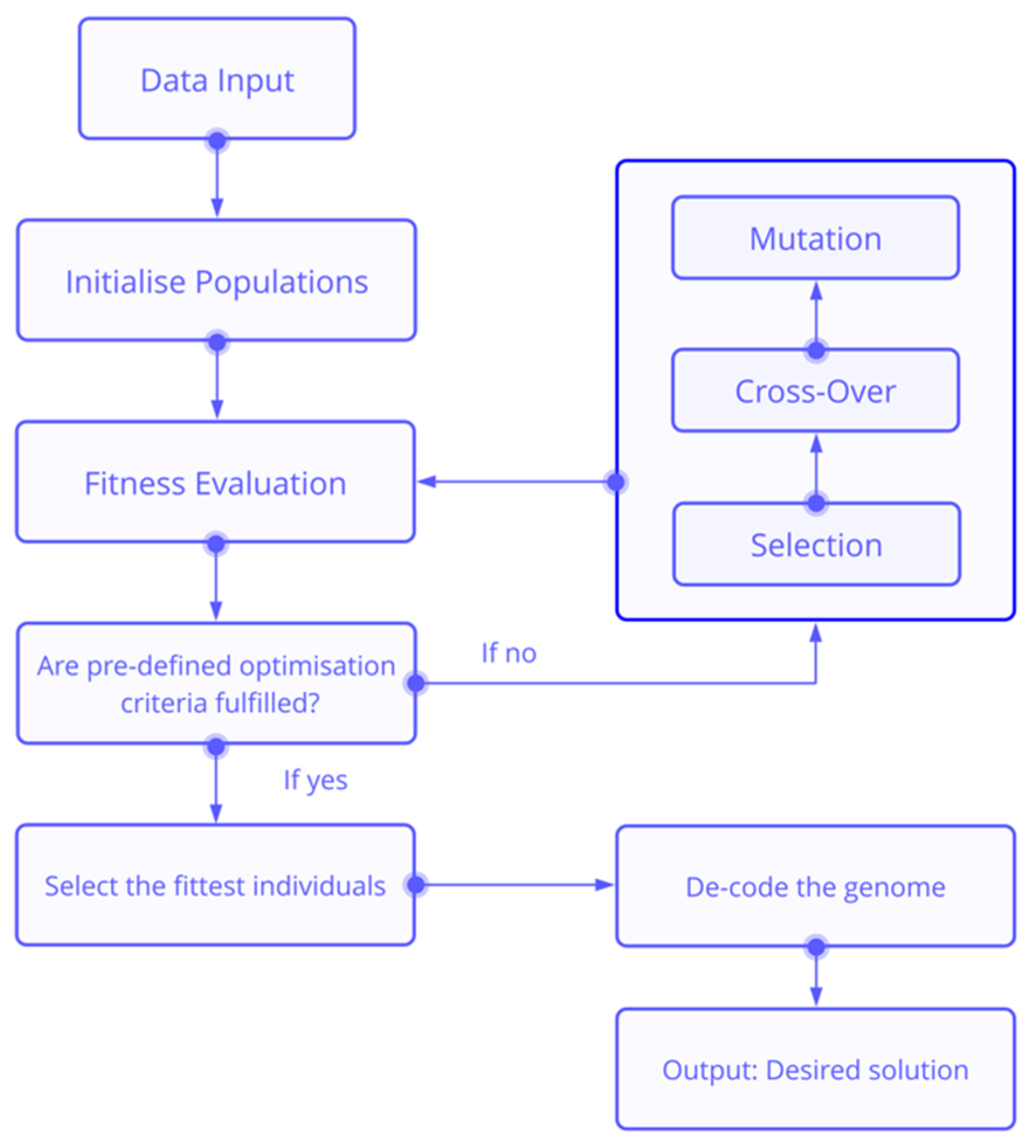
GA-evolved solutions are represented by a sequential encoding, i.e., the genome [35]. To find the best solution for any given problem and therefore, to evolve the best genome (=creation of the fittest individual), GAs uses bio-inspired, genetic processes such as selection, crossover and mutation [36]. A generic pseudo-code for genetic algorithms is depicted in Figure 2. The structure and design for the genome and therefore, the tools or building blocks to find a solution for any problem, might be tailored for each approach [14,37]. As for image classification, GAs can therefore help to automatically and efficiently find optimal solutions for CNN hyperparameter settings, as well as overall CNN architecture design [34]. Recently, GAs have demonstrated exceptional performance in automatically generating state-of-the-art CNNs—such as for classifying images of the CIFAR10 dataset with accuracies of up to 96.78 %, higher than most by DL experts manually tuned models [14]. Current research and recent advances of algorithms that can genetically design CNNs (CNN-GAs) do not only focus on algorithmic aspects such as variable-length encoding strategies with adaptive crossover operator length, but also address computational aspects, such as utilising all computational hardware resources efficiently to optimise computing time and costs [14].

In this paper, a genetic algorithm to automatically evolve and select the best CNN architecture design for classifying lung nodules from the Lung Image Database Consortium (LIDC) image collection was implemented by adopting both the proposed variable-length encoding and the proposed evolutionary operators by Sun et al. [14], to ultimately select the best-performing lung nodule classification model since naïve approaches of network architecture optimisation are not feasible, given the elevated amount of hyperparameters and other architectural features in CNN designs, such as layer count and type.

2. Materials and Methods

In this section, the design of the manually designed FractalNet and DLGN is presented. Furthermore, the design of the automatic CNN architecture design via genetic algorithm is described. All three models were configured and trained independently, with subsequent comparison of their respective classification performances on the validation data splits for cross validation.

In this study, all models were trained and validated with data sourced from the LIDC only. The sourced data consisted of thoracic CT scan files with additional annotations of a total of 1018 patients [8]. Utilised annotations included ratings of the nodules by radiologists ranging from 1 to 5, in which 1 indicates a low probability of the nodule’s malignancy and 5 indicates the highest chance for malignancy [38]. Examples for scans with different annotations for malignant nodules are displayed in Figure 3.

However, not all nodules were selected. The following criteria were applied to determine each sample’s inclusion and class membership for both the test and validation dataset: (a) at least 3 or more radiologists acknowledged the nodule with annotations; (b) each sample with a mean annotation value greater than 3 was labelled as ‘malignant’, otherwise as ‘benign’ if less than 3; and (c) samples with an average value of 3 were considered ‘ambiguous’ and therefore, were not to be included for training or validation purposes. Under those assumptions, 380 malignant and 421 benign nodules were identified. No further balancing of the dataset was performed, as the target class ratio of benign/malignant 1.07 indicates slight class imbalances only. To augment the dataset, further samples were created by following general DL conventions, such as rotating images by 90, 180 and 270 degrees. Furthermore, images were cropped from random sides with fixed stride, whilst relocating the centre of lung nodules as an area of interest. The described augmentation of the dataset was performed eight times.

For both FractalNet and CNN-GA training, a total of 6408 images were used—3040 of which were labelled as malignant, and 3368 labelled as benign. The first classification model, FractalNet, was implemented with the pre-processed dataset assorted into training and validation sets with a ratio of 8:2. With an overall total of 4 fractal blocks, a maximum pooling size of 2 and a convolutional filter size of 4, the training was performed for 50 epochs. The adjustment of weights was performed via the adaptive learning rate algorithm method (ADAM) with an initial learning rate of 0.002. Cross entropy was used for computing the loss function. The global drop probability was set 0.2. Dropout layers of the FractalNet were initialised with event probabilities of 0.1, 0.2, 0.3, 0.4 and 0.5, respectively. As the first layer was set with the lowest dropout probability, significant features are less likely to be overseen at the beginning of the convolutional training.

The same data split was utilised for the training and validation of the DLGN, the training of which was performed with a batch size of 150 for both 50 and 100 epochs. The comparison of target and output was conducted via binary cross entropy, whilst the subsequent adaption of weights was performed by using ADAM with an initial learning rate of 0.1. Generally, the linear transformations used in DLGN models characterise all regions of interest and analysed features, whilst Softmax classifiers are utilised to further extract regions with non-zero attention values.

For the CNN-GA, all digital imaging and communications in medicine (DICOM) files were transformed from the 3-channel RGB format with dimensions of 3 × 32 × 32 to greyscale NumPy arrays with dimensions of 1 × 32 × 32 each. The training-validation data split was randomised with rations between 10/90 and 60/40 for each performed CNN. Since the pre-processed CT-scans did not carry significant information which would be accessible by the RGB channel only, the transformation to the singular, monochrome format is not to impact classification performance whilst reducing the necessary use of computational resources. All generated monochrome NumPy arrays were subsequently transformed by using PyTorch. The pre-processed data were then converted into Tensor images with dimensions of 1 × 32 × 32 (input channels × height × width). Here, normalisation and additional, randomised horizontal flipping of all images was performed.

During the fitness evaluation, a fitness function evaluated all individuals per generation. Individuals whose genome encoded for CNNs with final validation performances below 50% were deemed unfit, and therefore were assigned a fitness score of 0. All other individual’s fitness values were derived by their classification performances using cross-validation.

The utilised GA design was developed to increase the depth of the CNN depth and therefore, its classification capability [14]. Hence, fully connected layers were replaced with skip layers, which can prevent the overfitting of the model. Following the mutation, the environmental selection was conducted by deploying the binary tournament selection approach, which is commonly used in single-objective optimisation with CNN-GAs [14,39].

Upon the selection of individuals, variable crossover and mutation relied on randomisation. Therefore, it was possible that, via genetic drift, the currently fittest individual and its corresponding genome may be deconstructed during either of the previously described random procedures [40]. Therefore, elitism was implemented by checking whether the fittest individual had already been selected to generate the new offspring for the next generation. If the fittest individual is not represented by the new parent generation yet, it will replace the least fit individual in the list of the current selection, which ensures the survival of the fittest individual. After each generation, a new population was initialised with all selected individuals and their freshly acquired genome. After evaluating and ranking all individuals according to their fitness, parents for the new generation were selected to generate new offspring for the new generation via mutation and crossover functions.

In this paper, CNN building blocks were implemented as per the proposal by Sun et al. shown in Figure 4.

The utilised genetic algorithm encodes CNN architectures with a variable genome length. This means that layer counts can vary, which gives more flexibility when adapting the overall network architecture. Please note that the resulting genome encodes pooling layers and skip layers, as this setup was inspired by Resnet’s architecture, which demonstrated high performances with the described skip layer-based network architecture [41,42].

3. Experimental Setup

The evolutionary simulation of the CNN-GA was initiated with a population count of n = 20. Each population inherited an initial fitness of zero. For each generation, each population was trained for 100 epochs with a subsequent mutation and crossover. All generated models were trained using stochastic gradient descent (SGD) with a learning rate of 0.1. Each training was followed by a fitness evaluation, in which all final validation accuracies of the current models were compared.

The probability of evolving the architecture with an additional skip layer by random mutation was furthermore set to be seven-fold higher than other possible mutations, which included adding pooling layers with random settings, removing layers, and changing hyperparameters of the currently encoded CNN design with all its components [14,30].

Randomised values for layer counts were generated within pre-determined convolutional layers count of min = 5, max = 15, with output channels generated between min = 64 and max = 512. The number of convolutional layers for each network architecture design is to be changed using the genetic operators of the proposed GA, as well as each layer’s input channel dimensions.

Rectifier activation functions and batch normalisation were appended to each convolutional layer. The final classification of each iteration was generated using a SoftMax classifier for both target classes.

Each CNN architecture was predetermined to inherit three pooling layers, with an analogue setup as per convolutional layer channel limits. Pooling layers were initialised with a kernel size of 2 × 2 and a stride of 2.

Skip layers that connected the prior convolutional layers to the following convolutional layer were assigned filter sizes of 3 × 3 with a stride of 1.

After 19 generations, the algorithm was set to terminate the evolutionary process, and the performance of populations throughout all generations as well as classification performance of all generated architectures were evaluated. For comparison purposes, FractalNet [22,24] and DGLNs [25,43] were used to compare with the CNN-GA. Cross-entropy was deployed with pytorch, using

$$loss\left(x,y\right)=-{{\displaystyle \sum }}^{ }x\log \left(y\right)$$

(1)

to compute loss the functions in this paper.

Notation 1. Cross-entropy loss function.

x = the label’s probability; y = the predicted label’s probability

All here-presented solutions that were generated by the CNN-GA were tracked using an individual identifier, as well as their generation count, whilst the generation count is indexed with 0 for the first generation: i.e., the ID 09-02 corresponds to the genomic encoding of the solution of individual number 2 in the 10th generation, the ID 01-15 corresponds to individual number 15 in the second generation, etc.

4. Results

The FractalNet training accuracy peaked at 87% during the 46th epoch of training. The final classification performance was 85% with a loss of 36% for cross-validation. After subsequently increasing the batch size, the performance was further reduced. Increasing the number of filters of the convolution layers did not result in testing accuracy. Upon increasing the learning rate by 50% (to 0.003), the accuracy was reduced furthermore.

The DGLN demonstrated a final classification performance of up to 92% during training. However, validation accuracy was significantly lower at 81%. Its performance during the validation was less constant, whilst the training accuracy improved more constantly over time. As for the training over 100 epochs, the classification accuracy plateaued and fluctuated between 80% and 90% with a final validation accuracy of 88.2%. However, the loss function did not approximate its final plateau after 100 iterations.

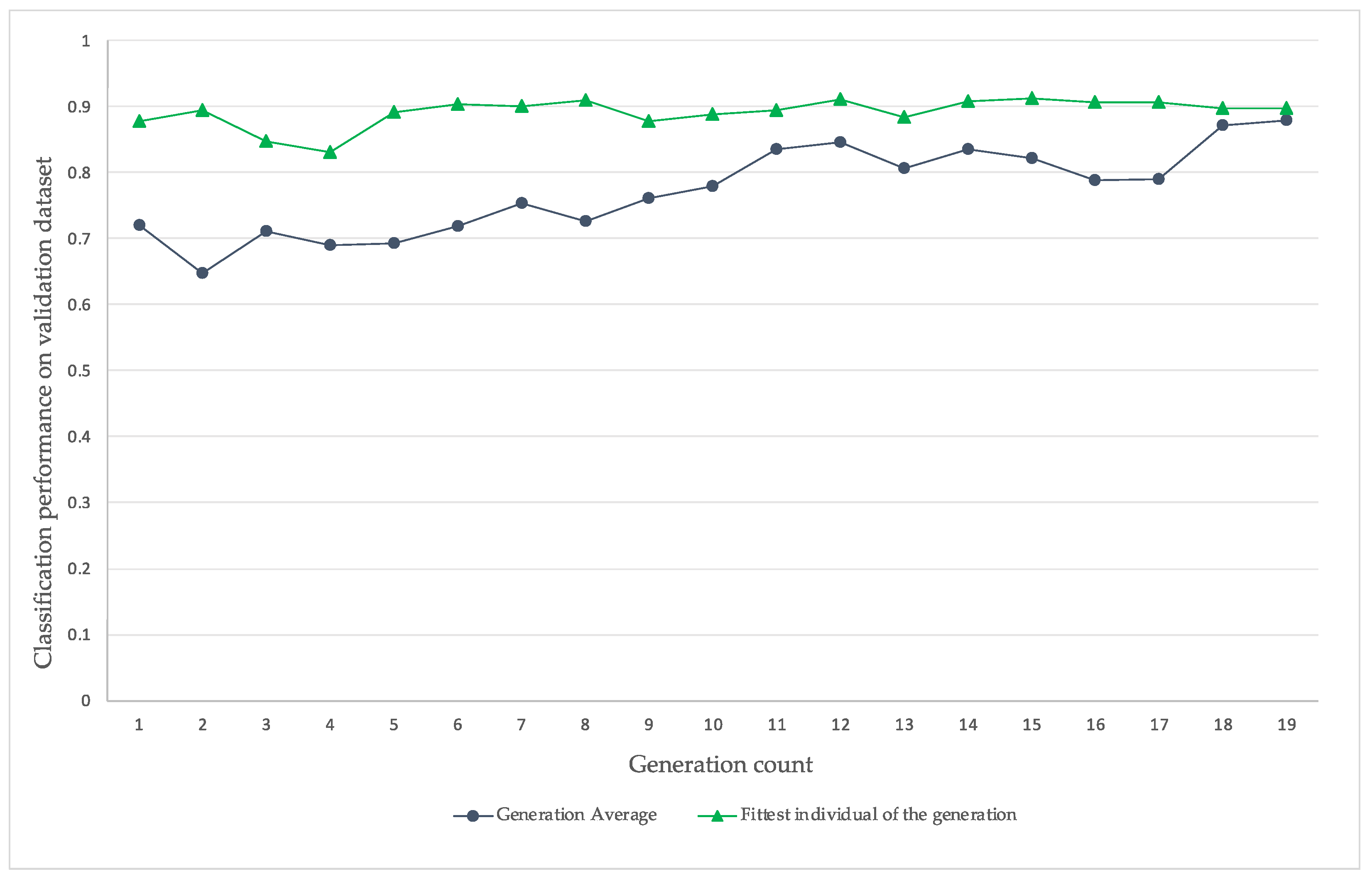
The CNN-GA was able to generate models with classification accuracies for training and validation data of up to 96.5% and 91.3%, respectively, the best-performing network architecture of which is depicted in Figure 5. Throughout the evolutionary process, underperforming individuals with elevated loss functions were eliminated. The summary of the population’s performance progression is shown in Figure 6. Note that the average final accuracy for each generation includes even the worst individuals of each generation, which was terminated prematurely due to their inability to classify.

The fittest individuals varied among the generations and therefore, the fittest individual was selected for each generation and plotted in Figure 6. Thus, the graph does not represent the classification performance progression of one single individual, i.e., one network architecture design solution. Despite having fit individuals with good performance after the first generation, the top performances improved only slowly over the course of 19 generations.

With the here utilised genomic encoding’s building blocks, the best classification performance on the validation dataset was achieved by a CNN with nine convolutional layers, and three pooling layers as shown in Figure 5.

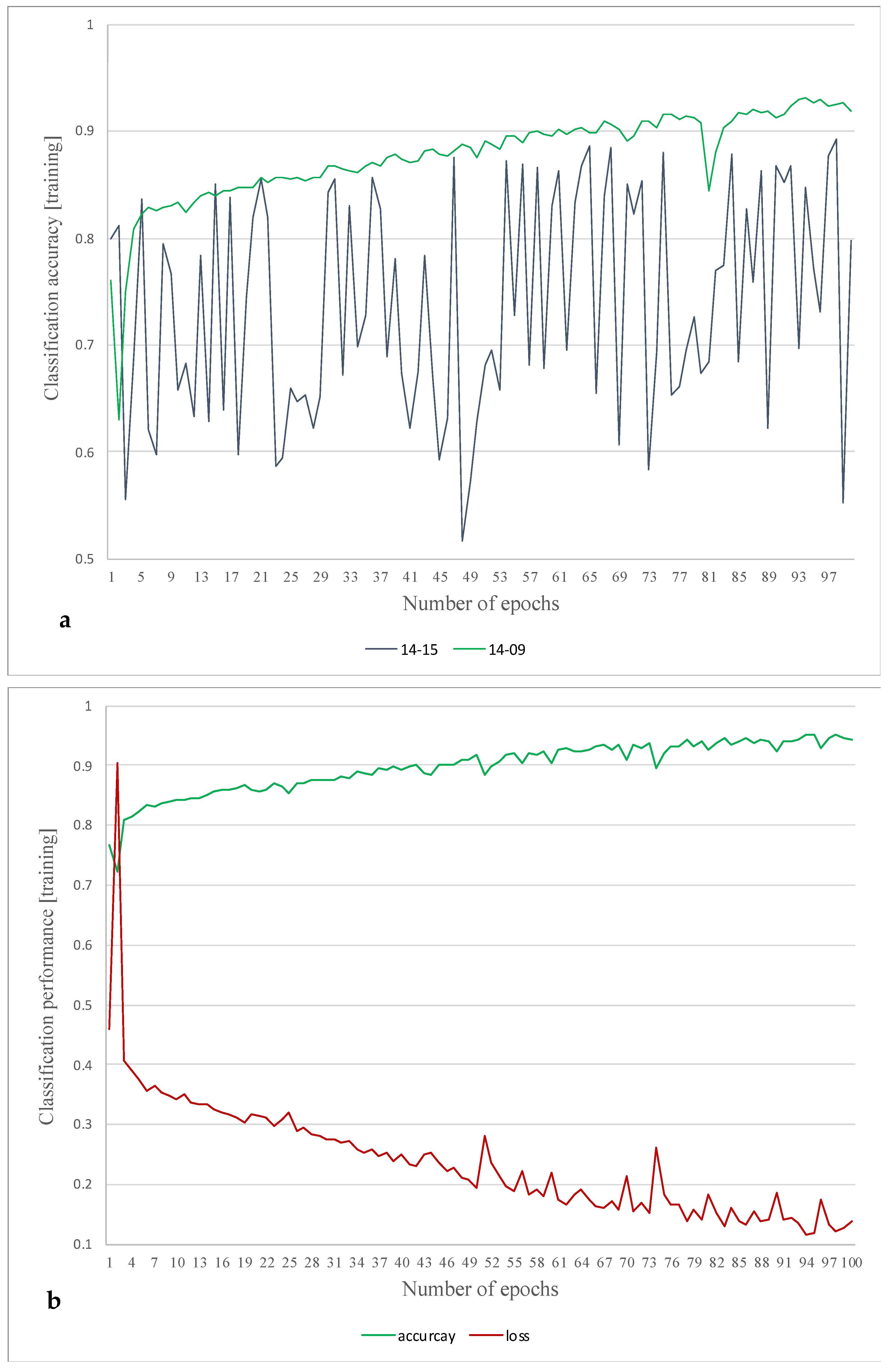
However, loss functions for validation datasets were significantly higher than their training data counterparts in most cases. Nonetheless, most models started to approximate a classification accuracy of more than 80% after evolving more than 9 generations. Many individuals remained unreliable despite demonstrating satisfactory final performances. As exemplarily shown in Figure 7, accuracies showed stark fluctuations across certain models training.

5. Discussion

Both the manually designed and off-the-shelf CNN can demonstrate respectable classification performance on hundreds of test cases within only one hour of computing, whilst the CNN-GA required over 79 h to compute the final CNN architecture, which demonstrated validation accuracies of over 91%. However, once the CNN-GA is well trained, its operation time is very fast. The comparison of all models is summarised in

Table 1. Comparison of the validation performances of all three models.

Method	Training Time [h]	Classification Accuracy [%]
FractalNet	1	82.0
Local-Global-Master	1	89.0
CNN-GA	79	91.3

.

To further improve the CNN-GA results, however, it is advisable to refrain from randomised data splitting, as the observed loss values showed stark variances for certain validation datasets. One may expect elevated validation accuracies if the CNN-GA was to be deployed with a fixed data split ratio. Additional runs would enable better a judgement of the CNN-GA’s reproducibility, which is not as high when compared to other classifiers since both evolutionary algorithms and the CNN training themselves rely heavily on randomised parameters [44]. Furthermore, the utilised SGD might be replaced by ADAM, since it is generally a more favourable choice for stochastic optimisation methods—particularly when facing noisy gradients [45].

The fittest individuals of the first generation accumulated a surprisingly high fitness of over 85%, and it is yet to prove that the relatively high mutation probability was favourable for optimising the evolutionary design approximation. To enhance classification reliability for future applications, decreased mutation probabilities could be set with an increased number of generations—even if such an approach would require significantly more time and perhaps, better computational resources.

To further develop the GA’s ability to find the best CNN architecture, additional building blocks may be added to the setup to boost the number of possible solutions of the gene pool. Whilst the used algorithm focuses on convolutional layer quantity and hyperparameter, it is recommended to investigate an evolutionary simulation that provides a ‘from scratch’ approach, which would allow adding a plethora of different layer types, hyperparameters, epochs, batch sizes, filters, learning rate methods, loss functions, and even automated data pre-processing structures.

6. Conclusions

In this paper, an implementation of a GA-designed, automated CNN architecture to address medical CT-imaging problems in lung cancer classification was successfully implemented, demonstrating that CNN-GAs can outperform manually tuned CNN classifiers, even in the absence of data-science expert knowledge. The proposed implementation of the CNN-GA for lung cancer classification may be deployed in various clinics in the future, as it may be possible to generate highly accurate, population-specific CAD tools for lung nodule malignancy classification on DICOM images with this approach.

The reproducibility of genetically evolved CNN classifiers may pose additional hurdles towards a full-on CAD implementation, as clear clinical and medical regulation standards are yet to be established in many countries [45,46,47]. Furthermore, the automatic design process of deep learning models adds an additional layer of concern to ethical hurdles, such as questions regarding the liability of the artificially generated CAD system [48]. In the future, one can expect clearer standards to arise, even for automatically generated CAD systems [49,50]. In the meantime, further research in the field of automatically designing CNN architectures with evolutionary algorithms is to be expected, with particular focus on optimizing reproducibility of the results for different populations. Additionally, further research may focus on speeding up CNN modelling and fitness evaluation to overcome computational limitations [14].

Overall, the outstanding performance of the GA-designed CNN classifier is an indicator for the future of deep learning and AI, with a plethora of possible applications outside of healthcare. The ability to develop optimised DL solutions in various fields, discrete of any field of interest with the given independence of machine learning expertise, may pave the way for a new era of developing AI.

Thus, being able to deploy optimised mathematical classifiers for various problems without being dependent on the presence of deep learning expertise has a high potential to coin the evolution of data-driven applications in the future and may increasingly drive new DL models to be discovered, the impact of which is yet to be defined. Accelerating computational performance (e.g., with quantum computing) in combination with computational optimisation (e.g., with population-based algorithms) may fundamentally change society and our relationship with computed intelligence.

References

1. National Cancer Institute. Non-Small Cell Lung Cancer Treatment (PDQ)—Patient Version. 2016. Available online: https://web.archive.org/web/20160229172247/http://www.cancer.gov/types/lung/patient/non-small-cell-lung-treatment-pdq (accessed on 30 May 2021).
2. Pasławski, M.; Krzyzanowski, K.; Złomaniec, J.; Gwizdak, J. Morphological characteristics of malignant solitary pulmonary nodules. Ann. Univ. Mariae Curie-Skłodowska Sect. D Med. 2004, 59, 6–13. [Google Scholar]
3. de Koning, H.J.; van der Aalst, C.M.; de Jong, P.A.; Scholten, E.T.; Nackaerts, K.; Heuvelmans, M.A.; Lammers, J.W.J.; Weenink, C.; Yousaf-Khan, U.; Horeweg, N.; et al. Reduced Lung-Cancer Mortality with Volume CT Screening in a Randomized Trial. N. Engl. J. Med. 2020, 382, 503–513. [Google Scholar] [CrossRef] [PubMed]
4. Australian Bureau of Statistics. 3303.0—Causes of Death, Australia, 2015. Available online: https://www.abs.gov.au/ausstats/[email protected]/Lookup/bySubject/3303.0~2015~MainFeatures~Lungcancer~10004 (accessed on 30 May 2021).
5. Ferlay, J.; Soerjomataram, I.; Dikshit, R.; Eser, S.; Mathers, C.; Rebelo, M.; Parkin, D.M.; Forman, D.; Bray, F. Cancer incidence and mortality worldwide: Sources, methods and major patterns in GLOBOCAN 2012. Int. J. Cancer 2015, 136, E359–E386. [Google Scholar] [CrossRef] [PubMed]
6. Knight, S.B.; Crosbie, P.A.; Balata, H.; Chudziak, J.; Hussell, T.; Dive, C. Progress and prospects of early detection in lung cancer. Open Biol. 2017, 7, 170070. [Google Scholar] [CrossRef] [PubMed] [Green Version]
7. OECD. Health at a Glance: Europe 2020, 19 November 2020. Available online: https://www.oecd-ilibrary.org/social-issues-migration-health/health-at-a-glance-europe-2020_82129230-en (accessed on 30 May 2021).
8. Lu, T.; Yang, X.; Huang, Y.; Zhao, M.; Li, M.; Ma, K.; Yin, J.; Zhan, C.; Wang, Q. Trends in the incidence, treatment, and survival of patients with lung cancer in the last four decades. Cancer Manag. Res. 2019, 11, 943–953. [Google Scholar] [CrossRef] [PubMed] [Green Version]
9. Merck, Lung Carcinoma: Tumors of the Lungs/Merck Manual Professional. 2007. Available online: https://web.archive.org/web/20070816142739/http://www.merck.com/mmpe/sec05/ch062/ch062b.html#sec05-ch062-ch062b-1405 (accessed on 30 May 2021).
10. Collins, L.G.; Haines, C.; Perkel, R.; Enck, R.E. Lung Cancer: Diagnosis and Management. Am. Fam. Physician. 2007, 75, 56–73. [Google Scholar] [PubMed]
11. Einav, L.; Finkelstein, A.; Mahoney, N. Provider Incentives and Healthcare Costs: Evidence From Long-Term Care Hospitals. Econometrica 2018, 86, 2161–2219. [Google Scholar] [CrossRef] [PubMed] [Green Version]
12. Messay, T.; Hardie, R.C.; Rogers, S.K. A new computationally efficient CAD system for pulmonary nodule detection in CT imagery. Med. Image Anal. 2010, 14, 390–406. [Google Scholar] [CrossRef]
13. Singadkar, G.; Mahajan, A.; Thakur, M.; Talbar, S. Deep Deconvolutional Residual Network Based Automatic Lung Nodule Segmentation. J. Digit. Imaging 2020, 33, 678–684. [Google Scholar] [CrossRef]
14. Sun, Y.; Xue, B.; Zhang, M.; Yen, G.G. Automatically Designing CNN Architectures Using Genetic Algorithm for Image Classification. arXiv 2018, arXiv:1808.03818. [Google Scholar] [CrossRef] [Green Version]
15. Vassanelli, S.; Mahmud, M. Trends and challenges in neuroengineering: Toward ‘intelligent’ neuroprostheses through brain-“brain inspired systems” communication. Front. Neurosci. 2016, 10, 438. [Google Scholar] [CrossRef] [PubMed]
16. Pesapane, F.; Codari, M.; Sardanelli, F. Artificial intelligence in medical imaging: Threat or opportunity? Radiologists again at the forefront of innovation in medicine. Eur. Radiol. Exp. 2018, 2, 1–10. [Google Scholar] [CrossRef] [PubMed] [Green Version]
17. Sahiner, B.; Pezeshk, A.; Hadjiiski, L.M.; Wang, X.; Drukker, K.; Cha, K.H.; Summers, R.M.; Giger, M.L. Deep learning in medical imaging and radiation therapy. Med. Phys. 2019, 46, e1–e36. [Google Scholar] [CrossRef] [PubMed] [Green Version]
18. Krizhevsky, A.; Sutskever, I.; Hinton, G.E. ImageNet Classification with Deep Convolutional Neural Networks. In Proceedings of the Conference on Neural Information Processing Systems (NIPS) on Machine Learning and Computational Neuroscience, Lake Tahoe, NV, USA, 3–8 December 2012. [Google Scholar]
19. Huang, G.; Liu, Z.; van der Maaten, L.; Weinberger, K.Q. Densely connected convolutional networks. In Proceedings of the 30th IEEE Conference on Computer Vision and Pattern Recognition, CVPR, Honolulu, HI, USA, 21–26 July 2017; pp. 2261–2269. [Google Scholar] [CrossRef] [Green Version]
20. Szegedy, C.; Liu, W.; Jia, Y.; Sermanet, P.; Reed, S.; Anguelov, D.; Erhan, D.; Vanhoucke, V.; Rabinovich, A. Going Deeper with Convolutions. In Proceedings of the IEEE Conference on Computer Vision and Pattern Recognition, Boston, MA, USA, 7–12 June 2015. [Google Scholar] [CrossRef] [Green Version]
21. Wu, P.; Sun, X.; Zhao, Z.; Wang, H.; Pan, S.; Schuller, B. Classification of Lung Nodules Based on Deep Residual Networks and Migration Learning. Comput. Intell. Neurosci. 2020, 2020, 8975078. [Google Scholar] [CrossRef] [PubMed]
22. Naik, A.; Edla, D.R.; Kuppili, V. Lung Nodule Classification on Computed Tomography Images Using Fractalnet. Wirel. Pers. Commun. 2021, 119, 1209–1229. [Google Scholar] [CrossRef]
23. Fu, J. Application of Modified Inception-ResNet and CondenseNet in Lung Nodule Classification. In Proceedings of the 3rd International Conference on Computer Engineering, Information Science & Application Technology, Chongqing, China, 30–31 May 2019; pp. 186–194. [Google Scholar] [CrossRef] [Green Version]
24. Al-Shabi, M.; Lan, B.L.; Chan, W.Y.; Ng, K.H.; Tan, M. Lung nodule classification using deep local-global networks. Int. J. Comput. Assist. Radiol. Surg. 2019, 14, 1815–1819. [Google Scholar] [CrossRef] [PubMed] [Green Version]
25. Larsson, G.; Maire, M.; Shakhnarovich, G. FractalNet: Ultra-deep neural networks without residuals. In Proceedings of the 5th International Conference on Learning Representations, ICLR, Toulon, France, 24–26 April 2017. [Google Scholar]
26. Zhang, H.; Goodfellow, I.; Metaxas, D.; Odena, A. Self-Attention Generative Adversarial Networks. PMLR 2019, 97, 7354–7363. [Google Scholar]
27. Young, S.R.; Rose, D.C.; Karnowski, T.P.; Lim, S.H.; Patton, R.M. Optimizing deep learning hyper-parameters through an evolutionary algorithm. In Proceedings of the Workshop on Machine Learning in High-Performance Computing Environments, Austin, TX, USA, 15 November 2015; pp. 1–5. [Google Scholar] [CrossRef]
28. Breuel, T.M. The Effects of Hyperparameters on SGD Training of Neural Networks. arXiv 2015, arXiv:1508.02788. [Google Scholar]
29. Turing, A.M.I. Computing Machinery and Intelligence; Oxford University Press on behalf of Mind: London, UK, 1950; Volume LIX, pp. 433–460. [Google Scholar] [CrossRef]
30. Srinivas, M.; Patnaik, L.M. Adaptive Probabilities of Crossover Genetic in Mu tation and Algorithms. IEEE Trans. Syste. Man Cybern. 1994, 24, 656–667. [Google Scholar] [CrossRef] [Green Version]
31. Sun, Y.; Yen, G.G.; Yi, Z. IGD Indicator-Based Evolutionary Algorithm for Many-Objective Optimization Problems. IEEE Trans. Evol. Comput. 2019, 23, 173–187. [Google Scholar] [CrossRef] [Green Version]
32. Stephenson, W. Number—The Language of Science. By Tobias Dantzig. London: George Allen & Unwin, Ltd., 1930. Large crown 8vo. Pp. 260. Price 10 s. J. Ment. Sci. 1931, 77, 843. [Google Scholar] [CrossRef]
33. Khuri, S.; Bäck, T.; Heitkotter, J. The zero/one multiple knapsack problem and genetic algorithms. In Proceedings of the ACM Symposium on Applied Computing, Phoenix, AZ, USA, 6–8 March 1994; Volume F129433, pp. 188–193. [Google Scholar] [CrossRef]
34. Hristakeva, M.; Shrestha, D. Solving the 0-1 Knapsack Problem with Genetic Algorithms. In Proceedings of the 2014 International Conference on Advanced Communication, Control and Computing Technologies (ICACCCT), Ramanathapuram, India, 8–10 May 2014. [Google Scholar]
35. Sivanandam, S.N.; Deepa, S.N. Genetic Algorithms. In Introduction to Genetic Algorithms; Springer: Berlin/Heidelberg, Germany, 2008; pp. 15–37. [Google Scholar]
36. Eiben, A.E.; Raué, P.E.; Ruttkay, Z. Genetic algorithms with multi-parent recombination. In Lecture Notes in Computer Science (Including Subseries Lecture Notes in Artificial Intelligence and Lecture Notes in Bioinformatics); Springer: Berlin/Heidelberg, Germany, 1994; Volume 866, pp. 78–87. [Google Scholar] [CrossRef]
37. Forrest, S. Genetic algorithms: Principles of natural selection applied to computation. Science 1993, 261, 872–878. [Google Scholar] [CrossRef] [PubMed] [Green Version]
38. Clark, K.; Vendt, B.; Smith, K.; Freymann, J.; Kirby, J.; Koppel, P.; Moore, S.; Phillips, S.; Maffitt, D.; Pringle, M.; et al. The Cancer Imaging Archive (TCIA): Maintaining and operating a public information repository. J. Digit. Imaging 2013, 26, 1045–1057. [Google Scholar] [CrossRef] [PubMed] [Green Version]
39. Miller, B.L.; Goldberg, D.E. Genetic Algorithms, Tournament Selection, and the Effects of Noise. Complex Syst. 1995, 9, 193–212. Available online: https://content.wolfram.com/uploads/sites/13/2018/02/09-3-2.pdf (accessed on 28 November 2021).
40. Du, H.; Wang, Z.; Zhan, W.; Guo, J. Elitism and distance strategy for selection of evolutionary algorithms. IEEE Access 2018, 6, 44531–44541. [Google Scholar] [CrossRef]
41. Liu, H.; Simonyan, K.; Vinyals, O.; Fernando, C.; Kavukcuoglu, K. Hierarchical representations for efficient architecture search. arXiv 2017, arXiv:1711.00436. [Google Scholar]
42. Real, E.; Moore, S.; Selle, A.; Saxena, S.; Suematsu, Y.L.; Tan, J.; Le, Q.V.; Kurakin, A. Large-Scale Evolution of Image Classifiers. In Proceedings of the International Conference on Machine Learning, Sydney, Australia, 6–11 August 2017; pp. 2902–2911. [Google Scholar] [CrossRef]
43. Cancer Imaging Archive. LIDC-IDRI—The Cancer Imaging Archive (TCIA) Public Access—Cancer Imaging Archive Wiki. 2021. Available online: https://wiki.cancerimagingarchive.net/display/Public/LIDC-IDRI (accessed on 21 May 2021).
44. Diethelm, K. The limits of reproducibility in numerical simulation. Comput. Sci. Eng. 2012, 14, 64–72. [Google Scholar] [CrossRef]
45. Hosny, A.; Parmar, C.; Quackenbush, J.; Schwartz, L.H.; Aerts, H.J.W.L.; Nature Publishing Group. Artificial intelligence in radiology. Nat. Rev. Cancer 2018, 18, 500–510. [Google Scholar] [CrossRef]
46. Vis, C.; Bührmann, L.; Riper, H.; Ossebaard, H.C. Health technology assessment frameworks for eHealth: A systematic review. Int. J. Technol. Assess. Health Care 2020, 36, 204–216. [Google Scholar] [CrossRef]
47. Salathé, M.; Wiegand, T.; Wenzel, M. Focus Group on Artificial Intelligence for Health; Fraunhofer-Institut für Nachrichtentechnik, Heinrich-Hertz-Institut: Berlin, Germany, 2018; Available online: https://www.researchgate.net/publication/327643779_Focus_Group_on_Artificial_Intelligence_for_Health/fulltext/5b9b2d4d92851ca9ed064891/Focus-Group-on-Artificial-Intelligence-for-Health.pdf?origin=publication_detail (accessed on 5 November 2021).
48. Prosperi, M.; Min, J.S.; Bian, J.; Modave, F. Big data hurdles in precision medicine and precision public health. BMC Med. Inform. Decis. Mak. 2018, 18, 139. [Google Scholar] [CrossRef]
49. Reddy, S.; Allan, S.; Coghlan, S.; Cooper, P. A governance model for the application of AI in health care. J. Am. Med. Inform. Assoc. 2000, 27, 491–497. [Google Scholar] [CrossRef] [PubMed]
50. Taylor, S.J.E.; Eldabi, T.; Monks, T.; Rabe, M.; Uhrmacher, A.M. Crisis, what crisis—Does reproducibility in modeling & simulation really matter? In Proceedings of the Winter Simulation Conference, National Harbor, MD, USA, 8–11 December 2019; pp. 749–762. [Google Scholar] [CrossRef] [Green Version]
Figure 1. Four consecutive thoracic CT scans (of a total of 112 scans) for one individual of the LIDC.
Signals 03 00018 g001
Figure 2. Generalised concept of genetic algorithms; based on natural selection of individuals for offspring creation, randomised cross-over and mutation lead to fit individuals.
Signals 03 00018 g002
Figure 3. Samples of malignant nodules (red) on CT scans of the LIDC, sorted via malignancy annotations from radiologists: (a) highly unlikely, (b) moderately unlikely, (c) indeterminate, (d) moderately suspicious, and (e) highly suspicious.
Signals 03 00018 g003
Figure 4. Conceptualised overview of one possible network architecture of the utilised GA’s building blocks with skip-connections (blue) between layers (orange). The grey hyperparameters of each layer are variable; the CNN network architecture shown here would be represented by the genome as “64-0.2-256-0.8-512”.
Signals 03 00018 g004
Figure 5. Building block-based CNN architecture with the best validation performance: fully convolutional network architecture with nine convolutional layers, one max pooling layer and two mean pooling layers.
Signals 03 00018 g005
Figure 6. Average and top validation performances of CNNs on for all populations during the evolutionary optimisation.
Signals 03 00018 g006
Figure 7. CNN-GA classification performance for selected individuals during training. (a) Selected individuals “15” and “09” from generation 15; (b) best-performing model overall of all 19 generations (individual identifier: 14–15).
Signals 03 00018 g007