
Constructing Features Using a Hybrid Genetic Algorithm

Abstract
1. Introduction
- Excessive computational times, because they require a processing time proportional to the dimension of the objective problem and the number of processing units as well. For example, a neural network of processing units applied to a test data with is considered an optimization problem with dimension . This means that the total number of network parameters is growing extremely quickly, which results in a longer computation time than the corresponding universal optimization method. An extensive discussion of the problems caused by the dimensionality of neural networks was presented in [24]. A common approach to overcome this problem is to use the PCA technique to reduce the dimensionality of the objective problem [25,26,27], i.e., the parameter d.
- The overfitting problem, which is quite common for these methods to produce poor results when they are applied to data (test data) not previously used in the training procedure. This problem was discussed in detail in the article by Geman et al. [28] as well as in the article of Hawkins [29]. A variety of methods have been proposed to overcome this problem, such as weight sharing [30], pruning [31,32,33], the dropout technique [34], early stopping [35,36], and weight decaying [37,38].
2. Method Description
2.1. The Usage of Grammatical Evolution
- N is the set of non-terminal symbols, which produce a series of terminal symbols through production rules.
- T is the set of terminal symbols.
- S is a non-terminal symbol which is also called the start symbol.
- P is a set of production rules in the form or .
- Every chromosome Z is split into parts. Each part will be used to construct a feature.
- For every part construct a feature using the grammar given in Figure 1.
- Create a mapping function:where is a pattern from the original set and Z is the chromosome.
2.2. Feature Construction
- Initialization step
- (a)
- Set iter = 0, generation number.
- (b)
- Construct the set , which is the original training set.
- (c)
- SetNc as the number of chromosomes and as the number of desired constructed features. These options are defined by the user.
- (d)
- Initialize randomly in range the integer chromosomes
- (e)
- Set as the maximum number of generations allowed.
- (f)
- Set as the selection rate and the mutation rate.
- Termination check. If iter ≥ go to step 6.
- Estimate the fitness of every chromosome with the following procedure:
- (a)
- Use the procedure described in Section 2.1 and create features.
- (b)
- Create a modified training set:
- (c)
- Train an RBF neural network C with H processing units on the modified training set using the following train error:
- Genetic Operators
- (a)
- Selection procedure: initially, the chromosomes are sorted according to their fitness value. The best chromosomes are placed in the beginning of the population and the worst at the end. The best chromosomes are transferred to the next generation intact. The remaining chromosomes are substituted by offspring created through the crossover and mutation procedures.
- (b)
- Crossover procedure: in this process, for every produced offspring, two mating chromosomes (parents) are selected from the previous population using tournament selection. Tournament selection is a rather simple selection mechanism defined as: first a set of randomly selected chromosomes is constructed and subsequently the chromosome with the best fitness value in the previous set is selected as the mating chromosome. Having selected the two parents for the offspring, the offspring is formed using the one point crossover. In one-point crossover, a random point is selected for the two parents and their right-hand side subchromosomes are exchanged.
- (c)
- Mutation procedure: for every element of each chromosome, a random number is taken. If , then this element is randomly altered by producing a new integer number.
- Set iter = iter + 1 and go to Step 2.
- Get the best chromosome in the population defined as with the corresponding fitness value and Terminate.
2.3. Weight Decay Mechanism
| Algorithm 1 Calculation of the bounding quantity for neural network |
|
2.4. Application of Genetic Algorithm
- Initialization step
- (a)
- Set iter = 0 as the generation number.
- (b)
- Set TN as the modified training set, where:
- (c)
- Initialize randomly the double precision chromosomes in range . The size of each chromosome is set to .
- Termination check. If iter ≥ Ng go to step 6
- Fitness calculation step.
- (a)
- For every chromosome :
- Calculate the quantity using Algorithm 1.
- Calculate the quantity , the training error of the neural network where the chromosome is used as the weight vector.
- Set, where as the fitness of .
- (b)
- End for
- Genetic operations step. Apply the same genetic operations as in the first algorithm of Section 2.2.
- Set iter = iter + 1 and go to step 2
- Local search step.
- (a)
- Get the best chromosome of the population.
- (b)
- For i = 1⋯W Do
- Set
- Set
- Set, .
- (c)
- End for
- (d)
- (e)
- Apply the optimized neural network to the test set, which has been modified using the same transformation procedure as in the train set, and report the final results.
3. Experiments
3.1. Experimental Datasets
- The Machine Learning Repository http://www.ics.uci.edu/~mlearn/MLRepository.html (accessed on 1 April 2022);
- The Keel Repository https://sci2s.ugr.es/keel/ (accessed on 1 April 2022).
- Balance dataset [62], used in psychological experiments.
- Dermatology dataset [63], which is used for differential diagnosis of erythemato-squamous diseases.
- Glass dataset. This dataset contains a glass component analysis for glass pieces that belong to 6 classes.
- Hayes Roth dataset [64].
- Heart dataset [65], used to detect heart disease.
- Parkinsons dataset [68], which is created using a range of biomedical voice measurements from 31 people, among which 23 have Parkinson’s disease (PD). The dataset has 22 features.
- Pima dataset, related to diabetes.
- PopFailures dataset [69], used in meteorology.
- Spiral dataset, which is an artificial dataset with two classes. The features in the first class are constructed as: and for the second class the used equations are:
- Wdbc dataset, which contains data for breast tumors.
- As a real-world example, consider an EEG dataset described in [72,73] which is used here. This dataset consists of five sets (denoted as Z, O, N, F and S), each containing 100 single-channel EEG segments which each have 23.6 s duration. With different combinations of these sets, the produced datasets are Z_F_S, ZO_NF_S, ZONF_S.
- BK dataset. This dataset comes from smoothing methods in statistics [74] and is used to estimate the points scored per minute in a basketball game. The dataset has 96 patterns of 4 features each.
- BL dataset. This dataset can be downloaded from StatLib. It contains data from an experiment on the effects of machine adjustments on the time to count bolts. It contains 40 patters of 7 features each.
- Housing dataset, described in [75].
- Laser dataset, which is related to laser experiments.
- NT dataset [76], which is related to body temperature measurements.
- Quake dataset, used to estimate the strength of an earthquake.
- FA dataset, which contains a percentage of body fat and ten body circumference measurements. The goal is to fit body fat to the other measurements.
- PY dataset [77], used to learn quantitative structure–activity relationships (QSARs).
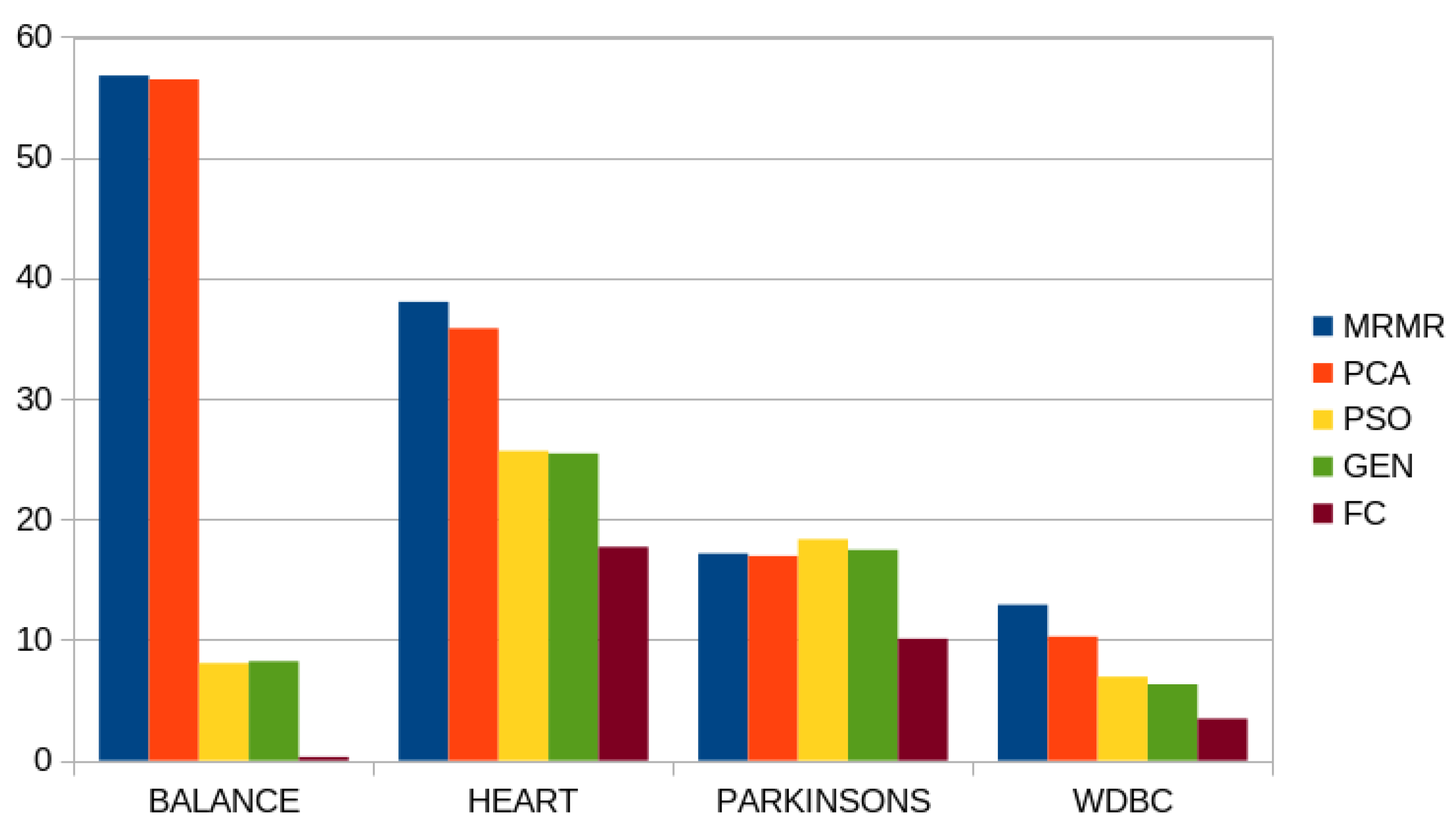
3.2. Experimental Results
- The principal component analysis (PCA) method as implemented in the Mlpack software [80]. The PCA method is used to construct two features from the original dataset. Subsequently, these features are evaluated using an artificial neural network trained by a genetic algorithm with chromosomes.
- A genetic algorithm with chromosomes and the parameters of Table 2 used to train a neural network with H hidden nodes. This approach is denoted as MLP GEN in the experimental tables.
- A particle swarm optimization (PSO) with particles and a number of generations used to train a neural network with H hidden nodes. This method is denoted as MLP PSO in the experimental tables.
4. Conclusions
Funding
Institutional Review Board Statement
Informed Consent Statement
Data Availability Statement
Conflicts of Interest
References
- Bishop, C. Neural Networks for Pattern Recognition; Oxford University Press: Oxford, UK, 1995. [Google Scholar]
- Cybenko, G. Approximation by superpositions of a sigmoidal function. Math. Control Signals Syst. 1989, 2, 303–314. [Google Scholar] [CrossRef]
- Baldi, P.; Cranmer, K.; Faucett, T.; Sadowski, P.; Whiteson, D. Parameterized neural networks for high-energy physics. Eur. Phys. J. C 2016, 76, 1–7. [Google Scholar] [CrossRef]
- Valdas, J.J.; Bonham-Carter, G. Time dependent neural network models for detecting changes of state in complex processes: Applications in earth sciences and astronomy. Neural Netw. 2006, 19, 196–207. [Google Scholar] [CrossRef]
- Carleo, G.; Troyer, M. Solving the quantum many-body problem with artificial neural networks. Science 2017, 355, 602–606. [Google Scholar] [CrossRef] [PubMed]
- Shen, L.; Wu, J.; Yang, W. Multiscale Quantum Mechanics/Molecular Mechanics Simulations with Neural Networks. J. Chem. Theory Comput. 2016, 12, 4934–4946. [Google Scholar] [CrossRef]
- Manzhos, S.; Dawes, R.; Carrington, T. Neural network-based approaches for building high dimensional and quantum dynamics-friendly potential energy surfaces. Int. J. Quantum Chem. 2015, 115, 1012–1020. [Google Scholar] [CrossRef]
- Wei, J.N.; Duvenaud, D.; Aspuru-Guzik, A. Neural Networks for the Prediction of Organic Chemistry Reactions. ACS Cent. Sci. 2016, 2, 725–732. [Google Scholar] [CrossRef]
- Falat, L.; Pancikova, L. Quantitative Modelling in Economics with Advanced Artificial Neural Networks. Procedia Econ. Financ. 2015, 34, 194–201. [Google Scholar] [CrossRef]
- Namazi, M.; Shokrolahi, A.; Maharluie, M.S. Detecting and ranking cash flow risk factors via artificial neural networks technique. J. Bus. Res. 2016, 69, 1801–1806. [Google Scholar] [CrossRef]
- Tkacz, G. Neural network forecasting of Canadian GDP growth. Int. J. Forecast. 2001, 17, 57–69. [Google Scholar] [CrossRef]
- Baskin, I.I.; Winkler, D.; Tetko, I.V. A renaissance of neural networks in drug discovery. Expert Opin. Drug Discov. 2016, 11, 785–795. [Google Scholar] [CrossRef] [PubMed]
- Bartzatt, R. Prediction of Novel Anti-Ebola Virus Compounds Utilizing Artificial Neural Network (ANN). Chem. Fac. 2018, 49, 16–34. [Google Scholar]
- Tsoulos, I.G.; Gavrilis, D.; Glavas, E. Neural network construction and training using grammatical evolution. Neurocomputing 2008, 72, 269–277. [Google Scholar] [CrossRef]
- Rumelhart, D.E.; Hinton, G.E.; Williams, R.J. Learning representations by back-propagating errors. Nature 1986, 323, 533–536. [Google Scholar] [CrossRef]
- Chen, T.; Zhong, S. Privacy-Preserving Backpropagation Neural Network Learning. IEEE Trans. Neural Netw. 2009, 20, 1554–1564. [Google Scholar] [CrossRef] [PubMed]
- Riedmiller, M.; Braun, H. A Direct Adaptive Method for Faster Backpropagation Learning: The RPROP algorithm. In Proceedings of the IEEE International Conference on Neural Networks, San Francisco, CA, USA, 28 March–1 April 1993; pp. 586–591. [Google Scholar]
- Pajchrowski, T.; Zawirski, K.; Nowopolski, K. Neural Speed Controller Trained Online by Means of Modified RPROP Algorithm. IEEE Trans. Ind. Inform. 2015, 11, 560–568. [Google Scholar] [CrossRef]
- Hermanto, R.P.S.; Nugroho, A. Waiting-Time Estimation in Bank Customer Queues using RPROP Neural Networks. Procedia Comput. Sci. 2018, 135, 35–42. [Google Scholar] [CrossRef]
- Robitaille, B.; Marcos, B.; Veillette, M.; Payre, G. Modified quasi-Newton methods for training neural networks. Comput. Chem. Eng. 1996, 20, 1133–1140. [Google Scholar] [CrossRef]
- Liu, Q.; Liu, J.; Sang, R.; Li, J.; Zhang, T.; Zhang, Q. Fast Neural Network Training on FPGA Using Quasi–Newton Optimization Method. IEEE Trans. Very Large Scale Integr. (VLSI) Syst. 2018, 26, 1575–1579. [Google Scholar] [CrossRef]
- Zhang, C.; Shao, H.; Li, Y. Particle swarm optimisation for evolving artificial neural network. In Proceedings of the IEEE International Conference on Systems, Man, and Cybernetics, Melbourne, Australia, 17–20 October 2000; pp. 2487–2490. [Google Scholar]
- Yu, J.; Wang, S.; Xi, L. Evolving artificial neural networks using an improved PSO and DPSO. Neurocomputing 2008, 71, 1054–1060. [Google Scholar] [CrossRef]
- Verleysen, M.; Francois, D.; Simon, G.; Wertz, V. On the Effects of Dimensionality on Data Analysis with Neural Networks. In Artificial Neural Nets Problem Solving Methods; IWANN 2003; Lecture Notes in Computer Science; Mira, J., Alvarez, J.R., Eds.; Springer: Berlin/Heidelberg, Germany, 2003; Volume 2687. [Google Scholar]
- Erkmen, B.; Yıldırım, T. Improving classification performance of sonar targets by applying general regression neural network with PCA. Expert Syst. Appl. 2008, 35, 472–475. [Google Scholar] [CrossRef]
- Zhou, J.; Guo, A.; Celler, B.; Su, S. Fault detection and identification spanning multiple processes by integrating PCA with neural network. Appl. Soft Comput. 2014, 14, 4–11. [Google Scholar] [CrossRef]
- Kumar, G.R.; Nagamani, K.; Babu, G.A. A Framework of Dimensionality Reduction Utilizing PCA for Neural Network Prediction. In Advances in Data Science and Management; Lecture Notes on Data Engineering and Communications Technologies; Borah, S., Emilia Balas, V., Polkowski, Z., Eds.; Springer: Singapore, 2020; Volume 37. [Google Scholar]
- Geman, S.; Bienenstock, E.; Doursat, R. Neural networks and the bias/variance dilemma. Neural Comput. 1992, 4, 1–58. [Google Scholar] [CrossRef]
- Hawkins, D.M. The Problem of Overfitting. J. Chem. Inf. Comput. Sci. 2004, 44, 1–12. [Google Scholar] [CrossRef] [PubMed]
- Nowlan, S.J.; Hinton, G.E. Simplifying neural networks by soft weight sharing. Neural Comput. 1992, 4, 473–493. [Google Scholar] [CrossRef]
- Hanson, S.J.; Pratt, L.Y. Comparing biases for minimal network construction with back propagation. In Advances in Neural Information Processing Systems; Touretzky, D.S., Ed.; Morgan Kaufmann: San Mateo, CA, USA, 1989; Volume 1, pp. 177–185. [Google Scholar]
- Mozer, M.C.; Smolensky, P. Skeletonization: A technique for trimming the fat from a network via relevance assesmentt. In Advances in Neural Processing Systems; Touretzky, D.S., Ed.; Morgan Kaufmann: San Mateo, CA, USA, 1989; Volume 1, pp. 107–115. [Google Scholar]
- Augasta, M.; Kathirvalavakumar, T. Pruning algorithms of neural networks—A comparative study. Cent. Eur. Comput. Sci. 2003, 3, 105–115. [Google Scholar] [CrossRef]
- Srivastava, N.; Hinton, G.E.; Krizhevsky, A.; Sutskever, I.; Salakhutdinov, R.R. Dropout: A simple way to prevent neural networks from overfitting. J. Mach. Learn. Res. 2014, 15, 1929–1958. [Google Scholar]
- Prechelt, L. Automatic early stopping using cross validation: Quantifying the criteria. Neural Netw. 1998, 11, 761–767. [Google Scholar] [CrossRef]
- Wu, X.; Liu, J. A New Early Stopping Algorithm for Improving Neural Network Generalization. In Proceedings of the 2009 Second International Conference on Intelligent Computation Technology and Automation, Changsha, China, 10–11 October 2009; pp. 15–18. [Google Scholar]
- Treadgold, N.K.; Gedeon, T.D. Simulated annealing and weight decay in adaptive learning: The SARPROP algorithm. Ieee Transactions Neural Netw. 1998, 9, 662–668. [Google Scholar] [CrossRef]
- Carvalho, M.; Ludermir, T.B. Particle Swarm Optimization of Feed-Forward Neural Networks with Weight Decay. In Proceedings of the 2006 Sixth International Conference on Hybrid Intelligent Systems (HIS’06), Rio de Janeiro, Brazil, 13 December 2006; p. 5. [Google Scholar]
- Neill, M.O.; Ryan, C. Grammatical evolution. IEEE Trans. Evol. Comput. 2001, 5, 349–358. [Google Scholar] [CrossRef]
- Gavrilis, D.; Tsoulos, I.G. Evangelos Dermatas, Selecting and constructing features using grammatical evolution. Pattern Recognition Lett. 2008, 29, 1358–1365. [Google Scholar] [CrossRef]
- Gavrilis, D.; Tsoulos, I.G. Evangelos Dermatas, Neural Recognition and Genetic Features Selection for Robust Detection of E-Mail Spam. In Advances in Artificial Intelligence Volume 3955 of the Series Lecture Notes in Computer Science; Springer: Berlin/Heidelberg, Germany, 2006; pp. 498–501. [Google Scholar]
- Georgoulas, G.; Gavrilis, D.; Tsoulos, I.G.; Stylios, C.; Bernardes, J.; Groumpos, P.P. Novel approach for fetal heart rate classification introducing grammatical evolution. Biomed. Signal Process. Control. 2007, 2, 69–79. [Google Scholar] [CrossRef]
- Smart, O.; Tsoulos, I.G.; Gavrilis, D.; Georgoulas, G. Grammatical evolution for features of epileptic oscillations in clinical intracranial electroencephalograms. Expert Syst. Appl. 2011, 38, 9991–9999. [Google Scholar] [CrossRef] [PubMed][Green Version]
- Goldberg, D. Genetic Algorithms in Search, Optimization and Machine Learning; Addison-Wesley Publishing Company: Reading, MA, USA, 1989. [Google Scholar]
- Michaelewicz, Z. Genetic Algorithms + Data Structures = Evolution Programs; Springer: Berlin, Germany, 1996. [Google Scholar]
- Doorly, D.J.; Peiro, J. Supervised Parallel Genetic Algorithms in Aerodynamic Optimisation, Artificial Neural Nets and Genetic Algorithms; Springer: Vienna, Austria, 1997; pp. 229–233. [Google Scholar]
- Sarma, K.C. Hojjat Adeli, Bilevel Parallel Genetic Algorithms for Optimization of Large Steel Structures. Comput. -Aided Civil Infrastruct. Eng. 2001, 16, 295–304. [Google Scholar] [CrossRef]
- Fan, Y.; Jiang, T.; Evans, D.J. Volumetric segmentation of brain images using parallel genetic algorithms. IEEE Trans. Med. Imaging 2002, 21, 904–909. [Google Scholar]
- Leung, F.H.F.; Lam, H.K.; Ling, S.H.; Tam, P.S. Tuning of the structure and parameters of a neural network using an improved genetic algorithm. IEEE Trans. Neural Netw. 2003, 14, 79–88. [Google Scholar] [CrossRef]
- Sedki, A.; Ouazar, D.; Mazoudi, E.E. Evolving neural network using real coded genetic algorithm for daily rainfall–runoff forecasting. Expert Syst. Appl. 2009, 36, 4523–4527. [Google Scholar] [CrossRef]
- Majdi, A.; Beiki, M. Evolving neural network using a genetic algorithm for predicting the deformation modulus of rock masses. Int. J. Rock Mech. Min. Sci. 2010, 47, 246–253. [Google Scholar] [CrossRef]
- Smith, M.G.; Bull, L. Genetic Programming with a Genetic Algorithm for Feature Construction and Selection. Genet. Program Evolvable Mach 2005, 6, 265–281. [Google Scholar] [CrossRef]
- Neshatian, K.; Zhang, M.; Andreae, P. A Filter Approach to Multiple Feature Construction for Symbolic Learning Classifiers Using Genetic Programming. IEEE Trans. Evol. Comput. 2012, 16, 645–661. [Google Scholar] [CrossRef]
- Li, X.; Yin, M. Multiobjective Binary Biogeography Based Optimization for Feature Selection Using Gene Expression Data. IEEE Trans. Nanobiosci. 2013, 12, 343–353. [Google Scholar] [CrossRef] [PubMed]
- Ma, J.; Teng, G. A hybrid multiple feature construction approach for classification using Genetic Programming. Appl. Soft Comput. 2019, 80, 687–699. [Google Scholar] [CrossRef]
- Cover, T.M. Geometrical and statistical properties of systems of linear inequalities with applications in pattern recognition. IEEE Trans. Electron. Comput. EC 1965, 14, 326–334. [Google Scholar] [CrossRef]
- Park, J.; Sandberg, I.W. Universal Approximation Using Radial-Basis-Function Networks. Neural Comput. 1991, 3, 246–257. [Google Scholar] [CrossRef]
- Backus, J.W. The Syntax and Semantics of the Proposed International Algebraic Language of the Zurich ACM-GAMM Conference. In Proceedings of the International Conference on Information Processing, UNESCO, Paris, France, 15–20 June 1959; pp. 125–132. [Google Scholar]
- Powell, M.J.D. A Tolerant Algorithm for Linearly Constrained Optimization Calculations. Math. Program. 1989, 45, 547. [Google Scholar] [CrossRef]
- Fletcher, R. A new approach to variable metric algorithms. Comput. J. 1970, 13, 317–322. [Google Scholar] [CrossRef]
- Chandra, R.; Dagum, L.; Kohr, D.; Maydan, D.; Menon, J.M.R. Parallel Programming in OpenMP; Morgan Kaufmann Publishers Inc.: San Francisco, CA, USA, 2001. [Google Scholar]
- Shultz, T.; Mareschal, D.; Schmidt, W. Modeling Cognitive Development on Balance Scale Phenomena. Mach. Learn. 1994, 16, 59–88. [Google Scholar] [CrossRef]
- Demiroz, G.; Govenir, H.A.; Ilter, N. Learning Differential Diagnosis of Eryhemato-Squamous Diseases using Voting Feature Intervals. Artif. Intell. Med. 1998, 13, 147–165. [Google Scholar]
- Hayes-Roth, B.; Hayes-Roth, B.F. Concept learning and the recognition and classification of exemplars. J. Verbal Learn. Verbal Behav. 1977, 16, 321–338. [Google Scholar] [CrossRef]
- Kononenko, I.; Šimec, E.; Robnik-Šikonja, M. Overcoming the Myopia of Inductive Learning Algorithms with RELIEFF. Appl. Intell. 1997, 7, 39–55. [Google Scholar] [CrossRef]
- Dy, J.G.; Brodley, C.E. Feature Selection for Unsupervised Learning. J. Mach. Learn. Res. 2004, 5, 845–889. [Google Scholar]
- Perantonis, S.J.; Virvilis, V. Input Feature Extraction for Multilayered Perceptrons Using Supervised Principal Component Analysis. Neural Process. Lett. 1999, 10, 243–252. [Google Scholar] [CrossRef]
- Little, M.A.; McSharry, P.E.; Hunter, E.J.; Ramig, L.O. Suitability of dysphonia measurements for telemonitoring of Parkinson’s disease. IEEE Trans. Biomed. 2009, 56, 1015–1022. [Google Scholar] [CrossRef] [PubMed]
- Lucas, D.D.; Klein, R.; Tannahill, J.; Ivanova, D.; Brandon, S.; Domyancic, D.; Zhang, Y. Failure analysis of parameter-induced simulation crashes in climate models. Geosci. Model Dev. 2013, 6, 1157–1171. [Google Scholar] [CrossRef]
- Raymer, M.; Doom, T.E.; Kuhn, L.A.; Punch, W.F. Knowledge discovery in medical and biological datasets using a hybrid Bayes classifier/evolutionary algorithm. IEEE transactions on systems, man, and cybernetics. Part B Cybern. Publ. IEEE Syst. Man Cybern. Soc. 2003, 33, 802–813. [Google Scholar] [CrossRef] [PubMed]
- Zhong, P.; Fukushima, M. Regularized nonsmooth Newton method for multi-class support vector machines. Optim. Methods Furth. Softw. 2007, 22, 225–236. [Google Scholar] [CrossRef]
- Andrzejak, R.G.; Lehnertz, K.; Mormann, F.; Rieke, C.; David, P.; Elger, C.E. Indications of nonlinear deterministic and finite-dimensional structures in time series of brain electrical activity: Dependence on recording region and brain state. Phys. Rev. E 2001, 64, 061907. [Google Scholar] [CrossRef]
- Tzallas, A.T.; Tsipouras, M.G.; Fotiadis, D.I. Automatic Seizure Detection Based on Time-Frequency Analysis and Artificial Neural Networks. Comput. Neurosci. 2007, 2007, 80510. [Google Scholar] [CrossRef]
- Simonoff, J.S. Smooting Methods in Statistics; Springer: New York, NY, USA, 1996. [Google Scholar]
- Harrison, D.; Rubinfeld, D.L. Hedonic prices and the demand for clean ai. J. Environ. Econ. Manag. 1978, 5, 81–102. [Google Scholar] [CrossRef]
- Mackowiak, P.A.; Wasserman, S.S.; Levine, M.M. A critical appraisal of 98.6 degrees f, the upper limit of the normal body temperature, and other legacies of Carl Reinhold August Wunderlich. J. Amer. Med. Assoc. 1992, 268, 1578–1580. [Google Scholar] [CrossRef]
- King, R.D.; Muggleton, S.; Lewis, R.; Sternberg, M.J.E. Drug design by machine learning: The use of inductive logic programming to model the structure-activity relationships of trimethoprim analogues binding to dihydrofolate reductase. Proc. Nat. Acad. Sci. USA 1992, 89, 11322–11326. [Google Scholar] [CrossRef] [PubMed]
- Peng, H.; Long, F.; Ding, C. Feature selection based on mutual information: Criteria of max-dependency, max-relevance, and min-redundancy. IEEE Trans. Pattern Anal. Mach. Intell. 2005, 27, 1226–1238. [Google Scholar] [CrossRef]
- Ding, C.; Peng, H. Minimum redundancy feature selection from microarray gene expression data. J. Bioinform. Comput. Biol. 2005, 3, 185–205. [Google Scholar] [CrossRef] [PubMed]
- Curtin, R.R.; Cline, J.R.; Slagle, N.P.; March, W.B.; Ram, P.; Mehta, N.A.; Gray, A.G. MLPACK: A Scalable C++ Machine Learning Library. J. Mach. Learn. 2013, 14, 801–805. [Google Scholar]


| String | Chromosome | Operation |
|---|---|---|
| <expr> | 9,8,6,4,16,10,17,23,8,14 | |
| (<expr><op><expr>) | 8,6,4,16,10,17,23,8,14 | |
| (<terminal><op><expr>) | 6,4,16,10,17,23,8,14 | |
| (<xlist><op><expr>) | 4,16,10,17,23,8,14 | |
| (x2<op><expr>) | 16,10,17,23,8,14 | |
| (x2 + <expr>) | 10,17,23,8,14 | |
| (x2 + <func>(<expr>)) | 17,23,8,14 | |
| (x2 + cos(<expr>)) | 23,8,14 | |
| (x2 + cos(<terminal>)) | 8,14 | |
| (x2 + cos(<xlist>)) | 14 | |
| (x2 + cos(x3)) |
| Parameter | Value |
|---|---|
| H | 10 |
| 500 | |
| 2 | |
| 0.10 | |
| 0.05 | |
| 200 | |
| −10.0 | |
| 10.0 | |
| F | 20.0 |
| 100.0 | |
| 5.0 |
| Dataset | Features | Patterns |
|---|---|---|
| Balance | 4 | 625 |
| BK | 4 | 96 |
| BL | 7 | 41 |
| Dermatology | 34 | 359 |
| Glass | 9 | 214 |
| Hayes Roth | 5 | 132 |
| Heart | 13 | 270 |
| Housing | 13 | 506 |
| Ionosphere | 34 | 351 |
| Laser | 4 | 993 |
| NT | 2 | 131 |
| Parkinson’s | 22 | 195 |
| Pima | 8 | 768 |
| PopFailures | 18 | 540 |
| PY | 27 | 74 |
| Quake | 3 | 2178 |
| FA | 18 | 252 |
| Sprial | 2 | 2000 |
| Wine | 13 | 179 |
| Wdbc | 30 | 569 |
| Z_F_S | 21 | 300 |
| Z_O_N_F_S | 21 | 500 |
| ZO_NF_S | 21 | 500 |
| Dataset | MRMR | PCA | MLP GEN | MLP PSO | FC MLP |
|---|---|---|---|---|---|
| Balance | 56.80% | 56.48% | 8.23% | 8.07% | 0.30% |
| Dermatology | 68.54% | 62.11% | 10.01% | 17.57% | 4.98% |
| Glass | 58.35% | 50.16% | 58.03% | 57.35% | 45.84% |
| Hayes Roth | 61.21% | 61.13% | 35.26% | 36.69% | 23.26% |
| Heart | 38.04% | 35.84% | 25.46% | 25.67% | 17.71% |
| Ionosphere | 12.93% | 21.22% | 13.67% | 15.14% | 8.42% |
| Parkinson’s | 17.16% | 16.96% | 17.47% | 18.35% | 10.10% |
| Pima | 26.29% | 39.43% | 32.98% | 30.45% | 23.76% |
| PopFailures | 7.04% | 31.42% | 7.66% | 6.24% | 4.66% |
| Spiral | 44.87% | 45.94% | 45.71% | 42.10% | 26.53% |
| Wine | 30.73% | 30.39% | 20.82% | 19.31% | 7.31% |
| Wdbc | 12.91% | 10.28% | 6.32% | 6.95% | 3.47% |
| Z_F_S | 32.71% | 44.81% | 9.42% | 10.38% | 5.52% |
| Z_O_N_F_S | 43.04% | 56.45% | 60.38% | 63.56% | 31.20% |
| ZO_NF_S | 33.79% | 40.02% | 8.06% | 8.84% | 4.00% |
| Dataset | MRMR | PCA | MLP GEN | MLP PSO | FC MLP |
|---|---|---|---|---|---|
| BK | 0.03 | 0.17 | 0.21 | 0.15 | 0.03 |
| BL | 0.15 | 0.19 | 0.84 | 2.15 | 0.005 |
| Housing | 67.97 | 319.08 | 30.05 | 33.43 | 10.77 |
| Laser | 0.031 | 0.145 | 0.003 | 0.038 | 0.002 |
| NT | 1.79 | 0.69 | 1.11 | 0.03 | 0.01 |
| Quake | 0.06 | 0.59 | 0.07 | 0.28 | 0.03 |
| FA | 0.02 | 0.08 | 0.04 | 0.08 | 0.01 |
| PY | 1.56 | 0.30 | 0.21 | 0.07 | 0.02 |
| Dataset | ||||
|---|---|---|---|---|
| Heart | 21.26% | 21.34% | 18.73% | 17.71% |
| BK | 0.02 | 0.02 | 0.02 | 0.03 |
| BL | 0.02 | 0.02 | 0.01 | 0.005 |
| FA | 0.01 | 0.01 | 0.01 | 0.01 |
Publisher’s Note: MDPI stays neutral with regard to jurisdictional claims in published maps and institutional affiliations. |
© 2022 by the author. Licensee MDPI, Basel, Switzerland. This article is an open access article distributed under the terms and conditions of the Creative Commons Attribution (CC BY) license (https://creativecommons.org/licenses/by/4.0/).
Share and Cite
Tsoulos, I.G. Constructing Features Using a Hybrid Genetic Algorithm. Signals 2022, 3, 174-188. https://doi.org/10.3390/signals3020012
Tsoulos IG. Constructing Features Using a Hybrid Genetic Algorithm. Signals. 2022; 3(2):174-188. https://doi.org/10.3390/signals3020012
Chicago/Turabian StyleTsoulos, Ioannis G. 2022. "Constructing Features Using a Hybrid Genetic Algorithm" Signals 3, no. 2: 174-188. https://doi.org/10.3390/signals3020012
APA StyleTsoulos, I. G. (2022). Constructing Features Using a Hybrid Genetic Algorithm. Signals, 3(2), 174-188. https://doi.org/10.3390/signals3020012