PID Controller Parameter Tables for Time-Delayed Systems Optimized Using Hill-Climbing

Abstract

Several parameter tables for PID controllers are known from the literature, for the control of time-delayed systems. The best known is that of Ziegler and Nichols, but there are others also. In this publication, a parameter table is presented that minimizes the quality criteria IAE, ITAE and ISE for the control of time-delayed systems that can be identified with PTn systems. The controller output limitation is also taken into account. Since it is very computationally intensive to calculate these PID parameter sets, a well-known approach from the field of artificial intelligence was chosen. This was hill-climbing, which can find the parameter sets with much less computational effort than is needed for nested loops. With this method, the PID parameter tables for the minimized quality criteria were found and compared, each on the basis of many randomized starting parameter values. The application of the hill-climbing method shows rapid convergence. The parameters are discussed with two examples of time-delayed systems: a PT3 and a PT5. The results are regulated systems which show very good transient behavior. Furthermore, it is also possible to use the procedure presented for optimal PID parameters to control general, stable systems.

1. Introduction and Related Research

Different approaches are known regarding how to find PID controller parameters from the step responses of time-delayed systems. After setting, they result in stable control systems. However, the parameters must be further optimized afterwards. The first approach was the Ziegler–Nichols method [1], but several others also exist, for example the approach of Chien, Hrones and Reswick [2]. Most of these approaches are heuristic. Furthermore, various methods are used for the optimization of controllers.

In recent years, particle swarm optimization (PSO) methods [3,4,5,6,7,8,9] or other related methods [10,11,12,13,14] have also been used for general controller optimization. These also provide parameters for a good convergence of the solution. Many other optimization methods for control parameters are also known [15,16,17,18,19].

In [3,4,5], PSO algorithms for PID tuning for H∞ criteria were presented and discussed. It was shown that the algorithms converged well. Mechatronic systems were also regulated in [6,7]; as an example, the optimization of a PID controller was applied for a direct drive wheel [6]. In [8], another type of particle was introduced for the PSO algorithm. The new algorithm was successfully used for a nonlinear PID-controlled system. In [9], some other methods for optimizing PID parameters for angular and linear motion control of an autonomous vehicle were discussed, and PSO was evaluated as the most promising method. Further optimization methods from the field of artificial intelligence were used in [10]. There, a self-tuning PID temperature controller was presented, which is based on a neural network and adapts to the current weather conditions. In [11], a genetic algorithm was used for the optimization of PID controller parameters for the position control of an electro-hydraulic servo actuator.

However, for the calculation of a parameter table it is important to find very small local minima or even the absolute minima of criteria. PSO only finds local minima. Here, the PID parameters Kp, Ti and Td are treated as particles in three-dimensional space. On the basis of tuples of random starting values, they are recalculated accordingly from iteration to iteration with a three-dimensional velocity vector. PSO contains three components for each particle, which are weighted separately: the speed vector from the last iteration, a speed vector which points in the direction of the best criterion that was achieved with this particle and a speed vector which points in the direction of the best criterion of all particles. The last component is particularly important, because there the social behavior of the particles influences the calculation.

In this paper, the hill-climbing method [20] is used. This is another stochastic method for use in optimizing controllers, but it is related to PSO. The most important difference is that the particles are processed serially and not in parallel. In particular, due to the missing social velocity component of the individual particles, more local minimal criteria are found, and therefore the probability of finding smaller local minima is increased. Finally, the smallest of the minimal criteria is accepted as the result. This is shown below.

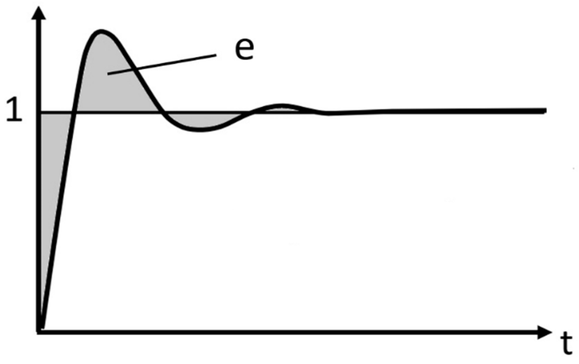
2. PTn Systems and ITAE, IAE and ISE Criteria

One method of representing time-delayed systems is with PTn systems. The control loop can be represented with a block diagram, as shown in Figure 1. The controller output is always limited in real systems, and the integrator of the controller is limited in most cases with an anti-windup.

PTn systems consist of series-connected PT1 (first-order) elements. Such systems are very common, and they can be found in all engineering disciplines. The series connection of the elements leads to delayed step responses. Thus, the time delay can be approximated with linear models. The measurement of the step response of a controlled system is identified using

Table 1. Table values, order n and T1 of the n PT1 systems, as a function of the delay time Tu and the rise time Tn [21].

PTn	PT2	PT3	PT4	PT5	PT6
Tg/Tu	9.71	4.61	3.14	2.44	2.03
Tg/T1	2.72	3.69	4.46	5.12	5.70
Tu/T1	0.28	0.8	1.42	2.10	2.81

. This is known from [21]. In many cases, one can simply measure the delay time Tu and the rise time Tg, according to Figure 2, by placing a tangent at the point of inflection. From this, one can identify the number n of PT1 elements connected in series and their identical time constants T1.

In addition to this method, there are also other methods by which the PTn systems can be identified using measurements. This problem has been solved and has been dealt with several times, for example in [22].

Figure 3 shows how the criteria are to be understood according to the step responses. The method uses the integral of the amount of the deviation of a step response from the unit step. IAE denotes ‘integral of absolute error’. Here, the amount of the error is integrated. In the figure, this corresponds to the area highlighted in gray. ITAE denotes ‘integral of time-multiplied absolute value of error’. In addition, the error is time-weighted in this case. This means that the integral grows faster over time. These criteria are also called the L1 criteria. The ISE criterion, the integral of the square value of the error, squares the error, and hence it increases more rapidly with larger errors. This criterion is also known as the L2 criterion.

$$\mathrm{IAE}:\underset{0}{\overset{\infty }{{\displaystyle \int }}}\left|\mathrm{e}\left(\mathrm{t}\right)-\mathrm{e}(\infty )\right|\mathrm{dt};\mathrm{ITAE}:\underset{0}{\overset{\infty }{{\displaystyle \int }}}\left|\mathrm{e}\left(\mathrm{t}\right)-\mathrm{e}(\infty )\right|·\mathrm{t}·\mathrm{dt};\mathrm{ISE}:\underset{0}{\overset{\infty }{{\displaystyle \int }}}{\left[\mathrm{e}\left(\mathrm{t}\right)-\mathrm{e}(\infty )\right]}^2\mathrm{dt}$$

(1)

3. The Hill-Climbing Method for Calculating the PID Controller Parameters

The controller parameters, according to the minimum IAE, ITAE and ISE criteria, can easily be calculated, in theory. To achieve this, all possible parameter combinations of P, I and D (Kp, Ti and Td) are simply simulated for several PTn controlled systems and various controller output limitations. Finally, the parameters with the smallest values are taken as the result. The parameters found in this way can then be stored in table form and used either in the simulation or directly in the practical system.

However, this method of calculation currently takes a very long time, due to the required computing power. The three parameters P, I and D span a three-dimensional space. For a single PTn element and a single controller output limitation, a total of (10 × 10)³ = 1,000,000 simulations would be necessary if the parameters were increased from 0.1 to 10 in steps of 0.1.

Therefore, a hill-climbing method, which is an artificial intelligence method, was selected for the parameter search [20]. First, random start values are generated for Kp, Ti and Td. They can be any value in the entire possible value range, here [0 … 10]. The parameters of the controller are changed according to a heuristic function. With each new calculation or measurement, the minimum change in the parameters ΔKp, ΔTi and ΔTd is multiplied by a random value from (+1, −1, 0). The change is added to the parameters. Then the criteria are recalculated. If the new value is smaller, the parameters are retained, and if not, the original parameters are recalculated. Figure 4 shows how the heuristic function acts on the PID controller parameters.

A flow chart of the method is shown in Figure 5. After a series of iterations, a termination criterion is met, which in the problem at hand was set to 500 (see also Figure 6).

Although the hill-climbing method converges quickly for this application, it cannot be guaranteed that the parameters for the absolutely smallest value of the criteria (e.g., IAE, ITAE, ISE) will be found in every case. The hill-climbing method, like the particle swarm optimization method, can end with parameters of local minima. However, since it requires much less computing time than calculating all parameter sets with nested loops, this approach was used here. In addition, a large number of completely randomly calculated starting values Kp, Ti and Td are assumed, and at the end of the comparison of the parameter sets the smallest are selected for the quality criteria. In fact, these calculations show fast convergence, and many of them result in the same PID parameter sets for the same smallest quality criteria of all calculated sets. As an example, the course of the convergence of the parameter Ti (PT2 system and ITAE criterion with a controller output limitation of +/−5), is shown in Figure 6.

In comparison with the PSO method, the biggest difference is that there, the particles move in parallel as tuples of Kp, Ti and Td through the definition space, and due to the social behavior speed component they show a stronger tendency to end together in local minima. With the hill-climbing method used here, the individual tuples are processed serially, according to the flow chart, and do not influence each other. This has the advantage that as many local minima as possible can be found, and then the smallest of these can be selected.

As discussed above, this method does not conclusively prove that these are really the parameter sets which absolutely minimize the quality criteria IAE, ITAE or ISE. However, a large number of randomized starting values were used, and a large number of these resulted in the same parameters for the minima of the ITAE, IAE or ISE criteria. It can therefore be assumed that these parameters either correspond to the optimal parameters or are at least very close to them. Furthermore, it is certain that these are excellent parameter sets that can be used immediately and effectively in practice.

4. Results: Calculated PID Parameters for the Minimized IAE, ITAE and ISE Criteria

Using the method described above, parameter sets for the general PTn controlled system are shown in

Table 2. PID parameters for minimized ITAE, IAE and ISE criteria.

PT1	+/−2	+/−3	+/−5	+/−10
IAE	Kp·Ks = 10	Kp·Ks = 10	Kp·Ks = 10	Kp·Ks = 10
IAE	Ti = 3.1·T1	Ti = 2·T1	Ti = 1.3·T1	Ti = 1·T1
IAE	Td = 0 (PI)	Td = 0 (PI)	Td = 0 (PI)	Td = 0 (PI)
ITAE	Kp·Ks = 9.3	Kp·Ks = 9.5	Kp·Ks = 9.1	Kp·Ks = 10
ITAE	Ti = 2.9·T1	Ti = 1.9·T1	Ti = 1.2·T1	Ti = 1·T1
ITAE	Td = 0 (PI)	Td = 0 (PI)	Td = 0 (PI)	Td = 0 (PI)
ISE	Kp·Ks = 10	Kp·Ks = 10	Kp·Ks = 9.8	Kp·Ks = 10
ISE	Ti = 2.7·T1	Ti = 1.6·T1	Ti = 1.5·T1	Ti = 0.2·T1
ISE	Td = 0 (PI)	Td = 0 (PI)	Td = 0 (PI)	Td = 0 (PI)
PT2, Tg/Tu = 9.71	+/−2	+/−3	+/−5	+/−10
IAE	Kp·Ks = 10	Kp·Ks = 10	Kp·Ks = 10	Kp·Ks = 10
IAE	Ti = 9.6·T1	Ti = 7.3·T1	Ti = 5.6·T1	Ti = 3.7·T1
IAE	Td = 0.3·T1	Td = 0.3·T1	Td = 0.3·T1	Td = 0.2·T1
ITAE	Kp·Ks = 10	Kp·Ks = 10	Kp·Ks = 9.6	Kp·Ks = 9.8
ITAE	Ti = 9.6·T1	Ti = 7.3·T1	Ti = 5.4·T1	Ti = 4.7·T1
ITAE	Td = 0.3·T1	Td = 0.3·T1	Td = 0.3·T1	Td = 0.3·T1
ISE	Kp·Ks = 10	Kp·Ks = 10	Kp·Ks = 10	Kp·Ks = 10
ISE	Ti = 9.7·T1	Ti = 7.3·T1	Ti = 5.1·T1	Ti = 4.6·T1
ISE	Td = 0.2·T1	Td = 0.2·T1	Td = 0.2·T1	Td = 0.1·T1
PT3, Tg/Tu = 3.61	+/−2	+/−3	+/−5	+/−10
IAE	Kp·Ks = 5.4	Kp·Ks = 7	Kp·Ks = 8.4	Kp·Ks = 10
IAE	Ti = 9.4·T1	Ti = 10·T1	Ti = 9.8·T1	Ti = 9.7·T1
IAE	Td = 0.7·T1	Td = 0.7·T1	Td = 0.7·T1	Td = 0.7·T1
ITAE	Kp·Ks = 5.4	Kp·Ks = 7	Kp·Ks = 8.2	Kp·Ks = 10
ITAE	Ti = 9.4·T1	Ti = 10·T1	Ti = 9.6·T1	Ti = 9.7·T1
ITAE	Td = 0.7·T1	Td = 0.7·T1	Td = 0.7·T1	Td = 0.7·T1
ISE	Kp·Ks = 6.1	Kp·Ks = 8.1	Kp·Ks = 10	Kp·Ks = 10
ISE	Ti = 10·T1	Ti = 9.8·T1	Ti = 10·T1	Ti = 7.8·T1
ISE	Td = 0.6·T1	Td = 0.6·T1	Td = 0.6·T1	Td = 0.6·T1
PT4, Tg/Tu = 3.14	+/−2	+/−3	+/−5	+/−10
IAE	Kp·Ks = 2	Kp·Ks = 2.9	Kp·Ks = 3.3	Kp·Ks = 3.3
IAE	Ti = 5.2·T1	Ti = 6.5·T1	Ti = 7.1·T1	Ti = 6.9·T1
IAE	Td = 1.1·T1	Td = 1.2·T1	Td = 1.3·T1	Td = 1.3·T1
ITAE	Kp·Ks = 1.9	Kp·Ks = 2.4	Kp·Ks = 2.3	Kp·Ks = 2.1
ITAE	Ti = 5·T1	Ti = 5.9·T1	Ti = 5.7·T1	Ti = 5·T1
ITAE	Td = 1.1·T1	Td = 1.2·T1	Td = 1.2·T1	Td = 1.1·T1
ISE	Kp·Ks = 2.8	Kp·Ks = 3.6	Kp·Ks = 4.9	Kp·Ks = 5.2
ISE	Ti = 6.6·T1	Ti = 7·T1	Ti = 7.1·T1	Ti = 7·T1
ISE	Td = 1.2·T1	Td = 1.2·T1	Td = 1.4·T1	Td = 1.4·T1
PT5, Tg/Tu = 2.44	+/−2	+/−3	+/−5	+/−10
IAE	Kp·Ks = 1.7	Kp·Ks = 1.8	Kp·Ks = 1.8	Kp·Ks = 1.7
IAE	Ti = 5.8·T1	Ti = 5.9·T1	Ti = 5.8·T1	Ti = 5.5·T1
IAE	Td = 1.6·T1	Td = 1.6·T1	Td = 1.6·T1	Td = 1.6·T1
ITAE	Kp·Ks = 1.4	Kp·Ks = 1.4	Kp·Ks = 1.4	Kp·Ks = 1.4
ITAE	Ti = 5.3·T1	Ti = 5.2·T1	Ti = 5.2·T1	Ti = 5.0·T1
ITAE	Td = 1.4·T1	Td = 1.4·T1	Td = 1.4·T1	Td = 1.4·T1
ISE	Kp·Ks = 1.9	Kp·Ks = 2.6	Kp·Ks = 2.5	Kp·Ks = 2.5
ISE	Ti = 5.9·T1	Ti = 6.5·T1	Ti = 6.3·T1	Ti = 6.1·T1
ISE	Td = 1.7·T1	Td = 1.8·T1	Td = 1.8·T1	Td = 1.8·T1
PT6, Tg/Tu = 2.03	+/−2	+/−3	+/−5	+/−10
IAE	Kp·Ks = 1.3	Kp·Ks = 1.3	Kp·Ks = 1.3	Kp·Ks = 1.3
IAE	Ti = 5.9·T1	Ti = 5.8·T1	Ti = 5.8·T1	Ti = 5.6·T1
IAE	Td = 1.9·T1	Td = 1.9·T1	Td = 1.9·T1	Td = 1.9·T1
ITAE	Kp·Ks = 1.1	Kp·Ks = 1.1	Kp·Ks = 1.1	Kp·Ks = 1.1
ITAE	Ti = 5.5·T1	Ti = 5.5·T1	Ti = 5.4·T1	Ti = 5.3·T1
ITAE	Td = 1.7·T1	Td = 1.7·T1	Td = 1.7·T1	Td = 1.7·T1
ISE	Kp·Ks = 1.8	Kp·Ks = 1.8	Kp·Ks = 1.8	Kp·Ks = 1.8
ISE	Ti = 6.8·T1	Ti = 6.5·T1	Ti = 6.5·T1	Ti = 6.3·T1
ISE	Td = 2.1·T1	Td = 2.1·T1	Td = 2.1·T1	Td = 2.1·T1

.

$$\mathrm{G}\left(\mathrm{s}\right)=\mathrm{Ks}·\frac{1}{{\left(\mathrm{s}·{\mathrm{T}}_1+1\right)}^{\mathrm{n}}}$$

Ks is the static gain, T₁ is the time constant and n is the number of PT1 elements connected in series. Ks, T₁ and n can be calculated, for example, from Figure 2 and Table 1, or by using other methods.

The results of this study were the following table values of the PID parameters for the minimum IAE, ITAE and ISE criteria of controlled PTn or time-delayed systems. Values from +/−2 to +/−10 are: (maximum controller output − controller output before the step) divided by (controller output for the stationary end value − controller output before the step). the maximum value of the table is limited to 10.

It is known from practice and theory that PTn systems with a higher order and thus a greater dead time (Tu) are more difficult to control. The PID controllers therefore require a higher D component (Td). The values from the table show very nicely that this also applies to the present parameters for minimizing the IAE, ITAE and ISE criteria.

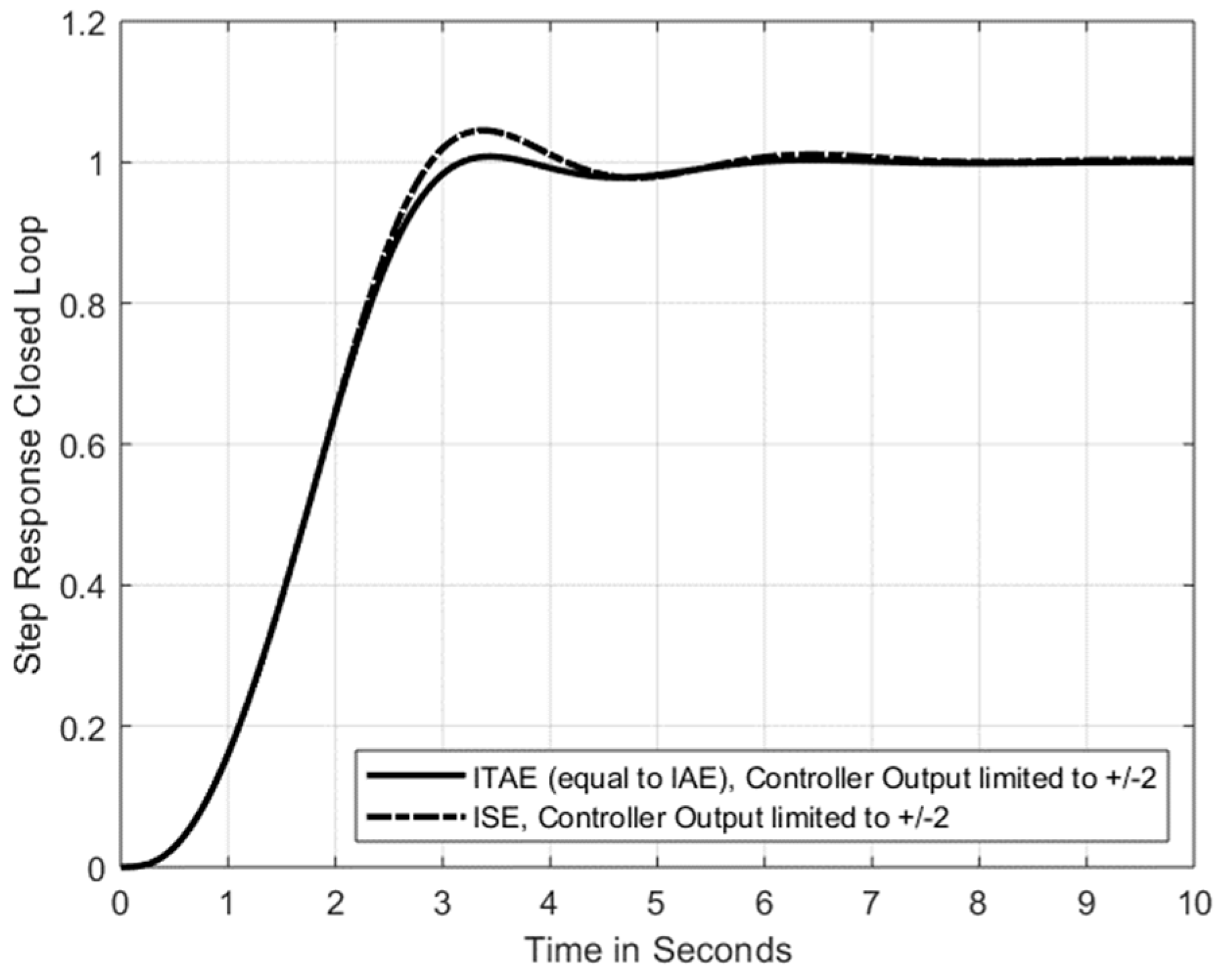
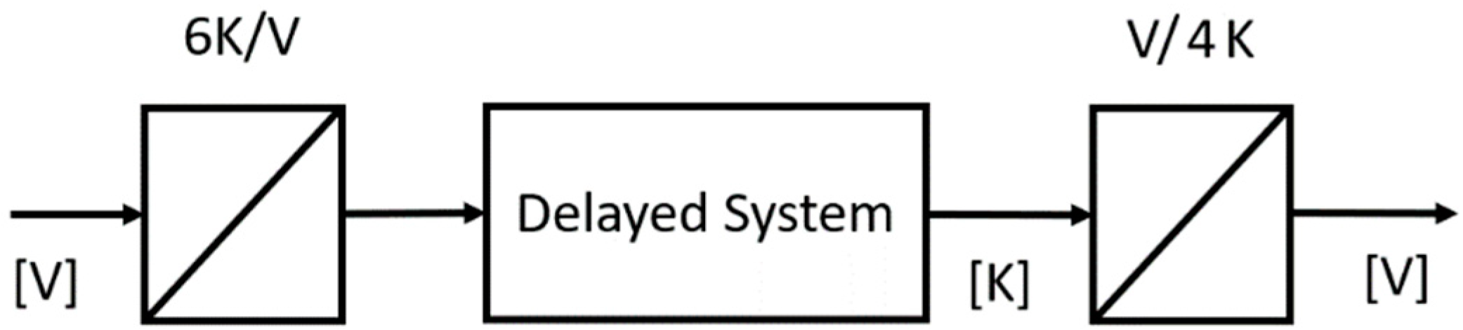
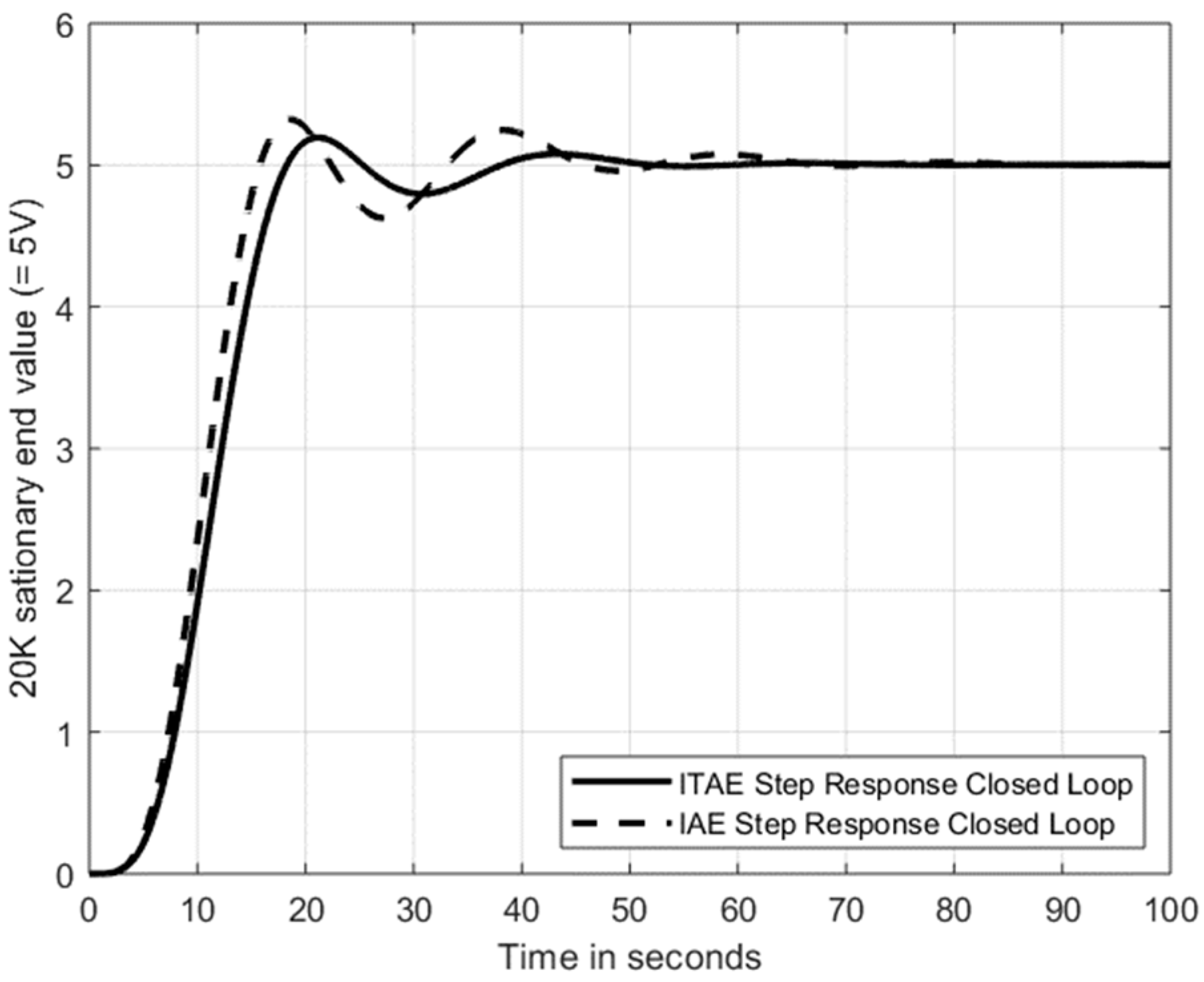
5. Applications for the Use of the Table: PID-Controlled PT3 and PT5

To show the correct use of the table, in the following, two examples were calculated and simulated. The controller structure was always in accordance with Figure 1 and the table values of Section 4. The two limitations must also be observed. Both the anti-windup and the controller output limitation were assumed to be the same. With the parameter sets according to Section 4, however, the anti-windup of the integral component is not actually necessary. This is never activated in the concrete examples, due to the controller output limitation and the use of the optimal parameters. Since it can occur in practice, for various reasons, that the actual value does not reach the setpoint, the anti-windup is nevertheless inserted here.

Example 1, control of a PT3 system (Tg/Tu = 4.61): for a PT3 system with T₁ = 1 s and Ks = 1, as well as an assumed controller output limitation of +/−2, the following PID parameters are read from the table.

For IAE and ITAE:

$$\mathrm{Kp}=\frac{5.4}{\mathrm{Ks}}=5.4\mathrm{Ti}=9.4·{\mathrm{T}}_1=9.4\mathrm{s}\mathrm{Td}=0.7·{\mathrm{T}}_1=0.7\mathrm{s}$$

For ISE:

$$\mathrm{Kp}=\frac{6.1}{\mathrm{Ks}}=6.1\mathrm{Ti}=10·{\mathrm{T}}_1=10\mathrm{s}\mathrm{Td}=0.6·{\mathrm{T}}_1=0.6\mathrm{s}$$

The response of the closed-loop system to a unit step, according to Figure 1, is shown in Figure 7 with these parameters.

Example 2, control of a real PT5 system, i.e., a temperature chamber: this example shows the application with Ks ≠ 1 and T₁ ≠ 1, as well as the correct use of the table with the controller output limitation. At this point, attention is also drawn to the special feature that the table values can be scaled with T₁ and Ks. This makes them usable for many applications. A thermal actuator heats a small heating chamber. For a biological experiment, the chamber should be heated from an initial temperature of 20 °C (outside temperature) to 40 °C. The temperature sensor in the chamber measures differentially in comparison to the outside temperature and has a linear characteristic with 1 V/4° K. The actuator is a coil, the power of which is linearized with an internal circuit and an amplifier. At the stationary end value, it heats the chamber at 6° K/1 V. The block diagram is shown in Figure 8.

For physical reasons, in a thermal system the heating reacts with a time delay. The system measures the step response of a jump from 0 V to 3.33 V. This results in a temperature difference ΔT = 20° K at the stationary end value or a voltage of 5 V in the differential sensor.

$$3.33\mathrm{V}·\frac{6°\mathrm{K}}{1\mathrm{V}}=20°\mathrm{K}\mathrm{or}3.33\mathrm{V}·\frac{6°\mathrm{K}}{1\mathrm{V}}·\frac{1\mathrm{V}}{4°\mathrm{K}}=5\mathrm{V}$$

The step response was measured from 0 V to 3.33 V under the same conditions and is shown in Figure 9.

The ratio Tg/Tu is 16/6.5 = 2.46. Using Table 1, this results in PT5 behavior. Since Tg/T1 = 5.12 (read from the table), this results in T₁ = 16 s/5.12, equal to approximately 3 s. To read off the correct table values, the controller output limitation is required. In this system this is +/−10 V. For a step of ΔT = 20° K, the controller output at the stationary end value is 3.3 V. This results in a controller output limitation of +/−10 V/3.3 V = +/−3. Ks is calculated as 5 V/3.3 V = 6° K/4° K = 1.5.

This results in the following PID parameters, according to Table 2.

For IAE:

$$\mathrm{Kp}=\frac{1.8}{\mathrm{Ks}}=1.2\mathrm{Ti}=5.9·{\mathrm{T}}_1=17.7\mathrm{s}\mathrm{Td}=1.6·{\mathrm{T}}_1=4.8\mathrm{s}$$

For ITAE:

$$\mathrm{Kp}=\frac{1.4}{\mathrm{Ks}}=0.93\mathrm{Ti}=5.2·{\mathrm{T}}_1=15.6\mathrm{s}\mathrm{Td}=1.4·{\mathrm{T}}_1=4.2\mathrm{s}$$

For ISE:

$$\mathrm{Kp}=\frac{2.6}{\mathrm{Ks}}=1.73\mathrm{Ti}=6.5·{\mathrm{T}}_1=19.5\mathrm{s}\mathrm{Td}=1.8·{\mathrm{T}}_1=5.4\mathrm{s}$$

In Figure 10, the closed-loop control step response for these calculations is shown, according to the block diagram in Figure 1.

6. Discussion and Outlook

The application of the hill-climbing method shows rapid convergence. The parameters found minimize the quality criteria ITA, IAE and ISE. They lead to regulated systems that show very good transient behavior. Furthermore, a PID parameter table for the control of PTn systems was calculated using this method.

The example of the PT3 system showed identical parameters for the optimal ITAE and IAE (L1) criteria. In fact, the optimal controller parameters of all criteria considered here for PTn systems of a smaller order were very close to one another. Since the quadratic error for deviations smaller than 1 is always smaller than the absolute error, a larger overshoot is permitted for the ISE (also L2) criterion than for IAE and ITAE. For this reason, the ISE generally shows a smaller attenuation of the system, because a small ripple, and also the time, are not strongly taken into account.

The example of the PT5 system is remarkable because such controlled systems with Tg/Tu = 2.44 are difficult to control using PID controllers, and they require optimal controller parameters. This shows the advantage of these optimal parameters according to the ITAE criterion. The time weighting ensures here that the system is sufficiently well damped. For the reasons mentioned above, the ISE criterion would have significantly poorer damping, which would not be useful in practice for the control of higher-order systems.

It is also shown that it makes sense to include the controller output limitation in the controller design. Thus, a good controller design and a good design regarding the physics are implemented in such a way that the controller output limitation is part of the system. Only in this way can the controller setup and the technical dimensioning of the system be carried out adequately.

With these sensibly selected PID controller parameters, PTn systems, which are relatively common in practice, can be controlled with very good results. Furthermore, because of the good convergence of the hill-climbing algorithm, it would also be possible to further automate the process and apply it directly to real systems, if the systems allow this with regard to stability.

References

1. Ziegler, J.G.; Nichols, N.B. Optimum settings for automatic controllers. ASME Trans. 1942, 64, 759–768. [Google Scholar] [CrossRef]
2. Chien, K.L.; Hrones, J.A.; Reswick, J.B. On the Automatic Control of Generalized Passive Systems. Trans. Am. Soc. Mech. Eng. ASME 1972, 74, 633–640. [Google Scholar]
3. Zamani, M.; Sadati, N.; Ghartemani, M.K. Design of H∞ PID controller using particle swarm optimization. Int. J. Control. Autom. Syst. 2009, 7, 273–280. [Google Scholar] [CrossRef]
4. Kim, T.-H.; Maruta, I.; Sugie, T. Robust PID controller tuning based on the constrained particle particle swarm optimization. Automatica 2008, 44, 1104–1110. [Google Scholar] [CrossRef]
5. Maruta, I.; Kim, T.-H.; Sugie, T. Fixed-structure H∞ controller synthesis: A meta-heuristic approach using simple constrained particle swarm optimization. Automatica 2009, 45, 553–559. [Google Scholar] [CrossRef]
6. Zhang, D.; Han, Q.-L.; Zhang, X.-M. Network-Based Modeling and Proportional–Integral Control for Direct-Drive-Wheel Systems in Wireless Network Environments. IEEE Trans. Cybern. 2020, 50, 2462–2474. [Google Scholar] [CrossRef] [PubMed]
7. Zhi, Q.; Shi, Q.; Zhang, H. Tuning of digital PID controllers using particle swarm optimization algorithm for a CAN-based DC motor subject to stochastic delays. IEEE Trans. Ind. Electron. 2019, 67, 5637–5646. [Google Scholar]
8. Chang, W.-D.; Shih, S.-P. PID controller design of nonlinear systems using an improved particle swarm optimization approach. Commun. Nonlinear Sci. Numer. Simul. 2010, 15, 3632–3639. [Google Scholar] [CrossRef]
9. Azar, A.T.; Ammar, H.H.; Ibrahim, Z.F.; Ibrahim, H.A.; Mohamed, N.A.; Taha, M.A. Implementation of PID controller with PSO tuning for autonomous vehicle. In Proceedings of the International Conference on Advanced Intelligent Systems and Informatics, Cairo, Egypt, 26–28 October 2019; Springer: Cham, Switzerland, 2019. [Google Scholar]
10. Liang, H.; Sang, Z.-K.; Wu, Y.-Z.; Zhang, Y.-H.; Zhao, R. High Precision Temperature Control Performance of a PID Neural Network-Controlled Heater Under Complex Outdoor Conditions. Appl. Therm. Eng. 2021, 195, 117234. [Google Scholar] [CrossRef]
11. Elbayomy, K.M.; Jiao, Z.; Zhang, H. PID controller optimization by GA and its performances on the electro-hydraulic servo control system. Chin. J. Aeronaut. 2008, 21, 378–384. [Google Scholar] [CrossRef] [Green Version]
12. Abbasi, E.; Naghavi, N. Offline auto-tuning of a PID controller using extended classifier system (XCS) algorithm. J. Adv. Comput. Eng. Technol. 2017, 3, 41–44. [Google Scholar]
13. Hussain, K.M.; Zepherin, R.A.; Shantha, M. Comparison of PID Controller Tuning Methods with Genetic Algorithm for FOPTD System. Int. J. Eng. Res. Appl. 2014, 4, 308–314. [Google Scholar]
14. Joseph, E.A.; Olaiya, O.O. Cohen- Coon PID Tuning Method, A Better Option to Ziegler Nichols- PID Tuning Method. Comput. Eng. Intell. Syst. 2017, 2, 141–145. [Google Scholar]
15. Ozana, S.; Docekal, T. PID Controller Design Based on Global Optimization Technique with Additional Constraints. J. Electr. Eng. 2016, 67, 160–168. [Google Scholar] [CrossRef] [Green Version]
16. Büchi, R. Modellierung und Regelung von Impact Drives für Positionierungen im Nanometerbereich. Doctoral Dissertation, ETH Zurich, Zurich, Switzerland, 1996. [Google Scholar]
17. da Silva, L.R.; Flesch, R.C.; Normey-Rico, J.E. Controlling industrial dead-time systems: When to use a PID or an advanced controller. ISA Trans. 2020, 99, 339–350. [Google Scholar] [CrossRef] [PubMed]
18. Martins, F.G. Tuning PID Controllers using the ITAE Criterion. Int. J. Eng. Educ. 2005, 21, 867–873. [Google Scholar]
19. Silva, G.J.; Datta, A.; Bhattacharyya, S.P. PID Controllers for Time-Delay Systems; Birkhäuser: Boston, MA, USA, 2005; ISBN 0-8176-4266-8. [Google Scholar]
20. Norvig, P. Artificial Intelligence: A Modern Approach, 2nd ed.; Prentice Hall: Upper Saddle River, NJ, USA, 2003; pp. 111–114. ISBN 0-13-790395-2. [Google Scholar]
21. Unbehauen, H. Regelungstechnik; Vieweg: Braunschweig, Germany, 1992. [Google Scholar]
22. Zacher, S.; Reuter, M. Regelungstechnik Für Ingenieure; Springer: Wiesbaden, Germany, 2017. [Google Scholar]
Figure 1. Block diagram with a PID-controlled PTn system.
Signals 03 00010 g001
Figure 2. Step response of a PTn system.
Signals 03 00010 g002
Figure 3. Illustration of the control error e(t) in the closed loop, as a basis for the IAE, ITAE and ISE criteria.
Signals 03 00010 g003
Figure 4. Heuristic function of hill-climbing method, acting on the PID controller parameters.
Signals 03 00010 g004
Figure 5. Flow chart of the hill-climbing method for finding the parameters Kp, Ti and Td.
Signals 03 00010 g005
Figure 6. Example of convergence of parameter Ti, for a PT2 system and ITAE criterion with a controller output limitation of +/−5. The initial random values 7.7 and 4.8 represent the two lines and converge both to the end value 5.4.
Signals 03 00010 g006
Figure 7. Step response of the controlled PT3 system of Example 1.
Signals 03 00010 g007
Figure 8. Block diagram of the temperature chamber including actuator and sensor.
Signals 03 00010 g008
Figure 9. Response of the heating chamber to a step from 0 V to 3.3 V.
Signals 03 00010 g009
Figure 10. PID control of the PT5 heating chamber, according to the optimal parameters for the IAE and ITAE criteria.
Signals 03 00010 g010