Abstract
Estimating the heart rate (HR) response to exercises of a given intensity without the need of direct measurement is an open problem of great interest. We propose here a model that can estimate the heart rate response to exercise of constant intensity and its subsequent recovery, based on soft computing techniques. Multilayer perceptron artificial neural networks (NN) are implemented and trained using raw HR time series data. Our model’s input and output are the beat-to-beat time intervals and the HR values, respectively. The numerical results are very encouraging, as they indicate a mean relative square error of the estimated HR values of the order of 10−4 and an absolute error as low as 1.19 beats per minute, on average. Our model has also been proven to be superior when compared with existing mathematical models that predict HR values by numerical simulation. Our study concludes that our NN model can efficiently predict the HR response to any constant exercise intensity, a fact that can have many important applications, not only in the area of medicine and cardio-vascular health, but also in the areas of rehabilitation, general fitness, and competitive sport.
1. Introduction
The heart rate (HR), i.e., the number of heart beats per minute, is probably the most informative cardiovascular variable. The analysis of the HR response to physical activities may provide valuable information regarding cardiovascular health, as it can detect hidden physiological responses or abnormalities. HR estimation is of great interest in pre-diagnostics, rehabilitation, recuperation as well as prevention of cardiovascular diseases [1].
Traditionally, the HR of a person may be monitored by use of an electrocardiogram (ECG), which requires multiple sensors attached to the body surface and is, thus, rather uncomfortable to the user [2,3]. Research on the field has been aimed at monitoring the HR from photoplethysmography (PPG) sensors, which are simple and may be embedded in wearable devices [2,3,4,5,6,7,8]. Several techniques have been developed for the HR monitoring from PPG signals, such as the processing of a raw PPG signal and a simultaneous acceleration signal [2], as well as the combination of short-time Fourier transform and spectral analysis (SFST) [4]. Moreover, a method based on Wiener filtering [5] and a particle filter-based algorithm [6] have been presented. Recently, estimation of HR through the phase information provided by the polar representation of PPG signals has been proposed [7].
This study focuses on the estimation of the HR response to exercise of various constant exercise intensities. Mathematical models based on exponential fitting or, more recent dynamical systems models based on a system of coupled ordinary differential equations, have been proposed for the numerical simulation and prediction of the HR response to exercise [9,10]. Several methods may be found in the literature for the estimation of the parameters involved in the HR variability signals [11,12,13]. A review of the most popular techniques for the time-frequency representation of the HR variability signals is presented in [11], whereas Khan et al. [12] compare the performance of five kernel-based time-frequency distributions in terms of their ability to estimate the instantaneous frequency of HR signals.
Estimating the HR response to any exercise intensity and any cardiovascular condition is an open problem and a challenging task. Thus, we believe that the implementation of neural networks (NNs) is an attractive alternative for the problem of HR estimation. It may be worth testing the performance of NN models to such problems, since NNs have proven to be very efficient in various medical applications. The implementation of NNs may be very effective as regards dynamic, real-time prediction of the HR, which is of utter importance, not only for the general public, but especially for population groups for which direct HR recordings at intense exercise are not possible or not allowed, such as elderly people and pregnant women.
Pertinent studies include, among others, the identification of the connection between exercise intensity and HR values [14], the estimation of the oxygen uptake from the HR values [15] and the prediction of the digoxin concentration for specific cardio-activities [16]. Furthermore, a feedforward NN has been proposed to reflect the effects of physical activity on the HR [17] and various NN models have been developed to monitor the HR and its variabilities from PPG signals [3,8].
Our study implements suitable Multilayer Perceptron (MLP) NNs to estimate the HR response to constant intensity exercise. The NNs are trained using beat-to-beat time intervals recorded during exercises of constant intensity. After describing the data collection process, as well as the basic steps of the NN modeling, we examine the performance of our proposed NN when compared to raw HR data of constant exercise intensity. We also provide a comparison between the estimated HR values provided by our NN model and the simulated values provided by a dynamical systems model [9,10].
2. Materials and Methods
2.1. Raw HR Measurements
The data collection [18] took place in the Department of Physical Activity and Sport of the Technical University of Madrid, Spain, under the approval of the local ethics committee. A written informed consent was signed by the participant before data collection. The present research meets the highest ethical standards and has been performed in accordance with the guidelines of the Helsinki Declaration of 1975, as revised in 2013 [19].
A healthy male (age 33, height 1.83 m and weight 82 kg) served as the test subject. His HR parameters were: hrmax = 185 beats per minute (bpm) and hrmin = 40 bpm; the former is defined as the highest HR value achieved in an all-out-effort to the point of exhaustion, whereas the latter refers to the HR at absolute rest [1]. The participant was a high-level professional runner, so he was able to keep the exercise intensity at constant levels and, thus, provide raw HR data of exceptional accuracy, as required by the study. He performed four running bouts of constant intensity exercise [9,10], ref. [18] followed by a passive recovery period, during which he laid horizontally and still on the floor. The experiment was carried out on a tartan track. Care was taken to ensure that the data recording environment was free of any additional electromagnetic signals, such as high-tension power lines, engines producing electromagnetic fields, or mobile phones.
The data recording protocol resulted in four sets of HR data, hereafter named as set (I), (II), (III), and (IV), respectively. Each set corresponds to the recorded HR response (beat-to-beat intervals) to exercises of constant intensity followed by a recovery period. The velocity of each exercise was measured by a Garmin Forerunner 201 GPS system and a Polar S625x speed-distance heart rate monitor. The latter provided measurements of the beat-to-beat time interval as well.
Table 1 presents the exercise intensity and the duration of each exercise/recovery set, whereas Figure 1 shows, as an example, the HR time series recorded during the second exercise and its subsequent recovery, i.e., set (II). In Figure 1, oscillations in the HR time series data can be observed, as is expected for any un-edited physiological signals. These oscillations are more pronounced in the recovery period, a fact that may be attributed to factors more apparent during recovery such as environmental or mental distractions. It should be noted here that the HR time series used in this study (as shown in Figure 1) underwent minimum editing, in order to preserve all information included in the raw data. Occasional errant data points that sporadically appeared due to technical or physiological reasons, such as missed/misread R or T waves, or abnormal ectopic beats, were excluded when their values were larger than 10 standard deviations from the local mean HR values [18].

Table 1.
Velocity and duration of each exercise set (the subscripts “ex” and “rec” refer to the exercise and recovery set, respectively).
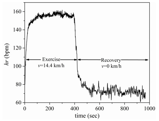
Figure 1.
Set (II) of HR time series data.
2.2. Neural Network Modelling
The block diagram of the NN model applied in this study is displayed in Figure 2. It consists of four pairs of NNs; each pair corresponds to an exercise set and its subsequent recovery at the specific velocity shown in the second column of Table 1. The NN architecture implemented for each block of Figure 2 is the MLP, which is a common choice for similar applications [16]. The input layer consists of one neuron, its input being the value of the beat-to-beat time interval, denoted as tbi, I = Iex, …, IVex or Irec, …, IVrec, whereas the output layer comprises a single neuron that sums the weighted outputs of the last hidden layer and produces the HR, i.e., hri. The specific structure of the MLP-NN applied for set (I)ex, i.e., for I = Iex, is shown in Figure 3; the circles denote the neurons in each layer.
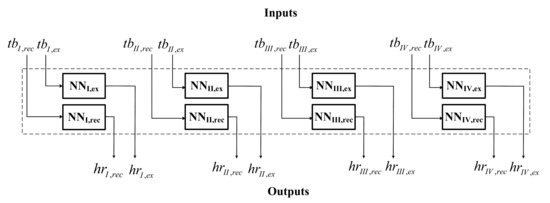
Figure 2.
Block diagram of the proposed NN model.
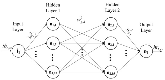
Figure 3.
Structure of the proposed MLP-NN for set (I)ex; the circles denote the neurons.
The appropriate number of hidden layers and the number of hidden neurons in each layer have been determined by applying a trial-and-error process. Both parameters are depicted in the second and third column of Table 2, respectively, for each exercise set. For example, the MLP-NN shown in Figure 3 consists of two hidden layers; the first one comprises 25 neurons, whereas the second one includes 15 hidden neurons. A logistic sigmoid activation function, given by , has been considered for all hidden layers, whereas a linear activation function has been selected for the neuron of the output layer [20,21,22,23,24]. The symbol (Figure 3) stands for the synaptic weight between the gth and the hth neuron, whereas the superscript j = 1, 2, 3 denotes the layer. The synaptic weights are adjustable parameters; at first, they are initialized and during training they are iteratively updated until the end of the training process. After training, their values remain constant [22,23,24].
Table 2.
MLP-NN parameters, MSEtr and M for each exercise set.
Simulations have been performed in MATLAB environment, where the NN toolbox has been used [25]. The first step into the estimation of the HR is taken by training the NNs. The four sets of HR data, collected as described in the previous subsection, were used to train the NNs. Although the data corresponds to one level of cardiovascular condition, it includes the response to various exercise intensities. Thus, the NNs were trained successfully to a sufficient number of cardiovascular stress levels and the corresponding ways of recovery. The training dataset consists of sample pairs , m = 1, 2, …, M, where represents the input, i.e., the values of the beat-to-beat time interval and stands for the desired output of the NN. Henceforth, the subscript or is omitted for the sake of brevity; and may belong to any exercise or recovery set. The integer M denotes the number of samples that compose the training dataset and is given in the last column of Table 2. Training of the MLP-NN has been carried out by using the Levenberg–Marquardt algorithm [22,23,24,25].
The performance of the training process is evaluated by calculating the training mean square error defined as follows:
where stands for the m-th predicted value of the HR by the NN and is the desired output of the NN, after the training process, as mentioned above. Τraining has been terminated when the number of epochs has reached its maximum value, which has been set equal to 1000. The achieved for each exercise set is given in the fourth column of Table 2. The latter suggests that is generally higher during the recovery than the exercise periods. This is a reasonable outcome, since HR decreases steeply during recovery, and it will be further discussed below.
A synoptic view of the whole procedure followed in this work, from HR data collection to the performance evaluation of the NNs, is displayed in Figure 4. The block on the left-hand side of the chart, enclosed in the dashed contour, refers to the data collection and processing, whereas the dashed block to the right includes the design, training, testing, and performance evaluation of the NN model.
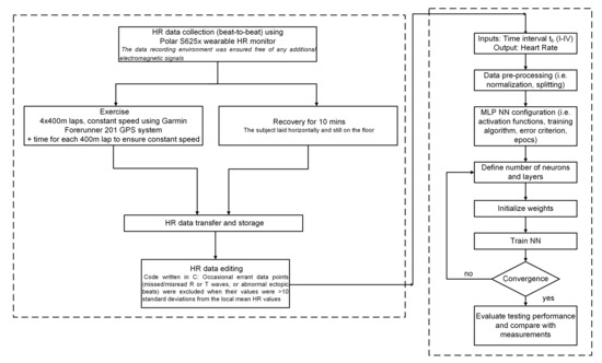
Figure 4.
Flow chart of the whole procedure from end to end.
2.3. Mathematical Analysis
The architecture of the single-input and single-output NN model proposed by the present study is equivalent to a non-linear function hr(t) that defines a mapping between two scalars, the beat-to-beat heart rate (hr) values and the time (t). Mathematical evaluations of this function have been proposed and extensively studied, as to their goodness of fit to raw HR data, as well as to their rigor and mathematical validity. In this sub-section, we will briefly reference the two main mathematical approaches, the exponential 3-phase model and the dynamical systems model (both discussed in more detail in [9,10]).
The 3-phase model has been emerged as the best fit to the data, from a statistical point of view. To simulate the body’s response to exercise, the hr values are calculated by use of the following exponential relation (the two last distinct terms are activated at the beginning of the last two phases):
where τ1, τ2, and τ3 are the time constants used to fit the exponentials, the parameters A1, A2, and A3 control the asymptotic HR values, and the constants TD2 and TD3 are the time delays that correspond to each one of the assumed phases. The hr values during recovery are modeled using one exponential.
It should be noted that much debate exists as to the validity of this model as, despite many attempts for a number of years, no convincing physiological mechanism for such discontinuous behavior has been proven to exist. It is very likely that the observed three phases are a figment of the incorrect and overly simple treatment of the data (such as averaging). Moreover, the above 3-phase model cannot be used for prediction, as the model’s parameters reflect the body’s physiological response to the particular exercise intensity only.
An alternative mathematical approach based on dynamical systems assumes the hr values to arise as solutions of the following set of coupled ordinary differential equations, regarding the rates of change of heart rate hr and velocity v:
where λ is a global parameter that defines the current cardio-vascular condition (takes values between 0 and 1), fmin and fmax are functions that act as repellers and control the dynamics near the minimum and the maximum heart rate respectively, fD is a function that acts as an attractor and controls the dynamics near the heart rate demand, and I(t) is the exercise intensity. In this dynamical systems model, the resulting hr is a smooth and continuous function of time, as no phases or time-delays in the body’s response to exercise are assumed to exist. This model is able to simulate and predict heart rate kinetics for any given exercise intensities. Examples of the HR values simulated by the above dynamical systems model are provided in the following section.
3. Results
The evaluation of the performance of the NN model proposed herein is the last step in the flow chart of Figure 4, as indicated by the block at the lower right-hand corner of the chart. The testing procedure is performed with an independent dataset, which is kept unseen from the NNs during training. The testing dataset comprises samples of the form , k = 1, 2, …, K with and being the input and the output, respectively, of the NN during testing; K stands for the number of samples used for testing. The testing mean absolute error is defined as follows:
whereas the testing relative mean square error is given by:
Both and have been calculated for all exercise sets; their values are listed in Table 3. The latter indicates that the may vary between 10−3 and 10−5, while the for all sets is 1.19 bpm on average; this is a satisfactory outcome, since results reported by other researchers, that employ techniques based on PPG signals to estimate HR, refer to average absolute errors of the order of 1.06 [4], 1.37 [5], 1.17 [6], 1 [7], and 1.03 [3] bpm.
Table 3.
MAEte, RMSEte, and K for each exercise set.
The main remark about Table 3 is that both the and the are smaller during the exercise than the recovery period for all sets presented herein; a similar remark has been reported for the . On average, the is 0.84 bpm during exercise, whereas it increases to 1.54 bpm for the recovery periods. As regards the , it deteriorates by roughly one order of magnitude for the recovery compared to the exercise periods. This may be attributed to the high non-linearity and the steep decrease of the HR during recovery, as well as to the inherent physiological noise, which is much more pronounced during the recovery than the exercise periods. Future work may focus on improving the accuracy of the model by applying the appropriate noise suppression techniques.
A comparison of the HR predicted from the NN models with measured HR time series data is presented in Figure 5, for the exercise and recovery periods of sets (I) and (II). It is readily apparent from Figure 5 that the proposed NN models are able to predict the HR accurately. Moreover, the familiar remark that the performance of the NNs is slightly better during the exercise than the recovery periods may be verified by the diagrams of Figure 5. Still, the overall performance of all NNs is of sufficient accuracy, since the does not exceed 10−3 for all cases examined, as indicated by Table 3.
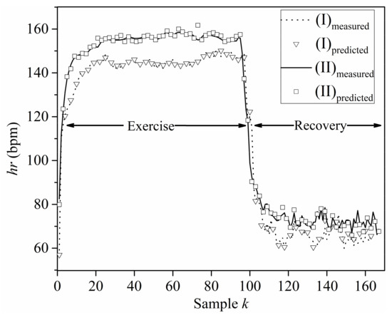
Figure 5.
Measured, , and predicted, , HR values for sets (I) and (II).
Figure 6 offers a comparison of results predicted by the proposed NN model (denoted as predicted hereafter) with the corresponding results produced by the mathematical model presented by Zakynthinaki [9,10] (denoted as simulated hereafter). The exercise and recovery periods of sets (III) and (IV) are considered, while the measured HR time series data (henceforth denoted as measured) are also included for reference. A careful examination of the results in Figure 6 leads to the conclusion that the NN model provides more accurate predictions than the mathematical model. This remark is more apparent from the plots for the recovery period, i.e., for k > 100; where the NN model is more efficient in capturing the frequent variations of the hr. It is worth mentioning that the dashed and dash-dotted lines in Figure 6 are representative examples of the HR values simulated by the dynamical systems model of Equation (3).
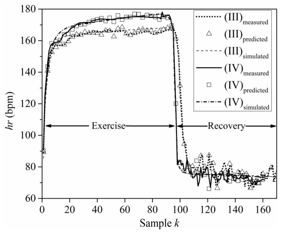
Figure 6.
Measured, predicted, and simulated HR values for sets (III) and (IV).
The superiority of the proposed NN model over the mathematical model [9,10] may be verified from Table 4, where the testing mean relative absolute error (MRAE) is given for all datasets. The predicted MRAE, displayed in the second column of Table 4, is defined as follows:
where stands for the k-th predicted value of the HR by the NN and is the corresponding k-th measured value. The simulated MRAE, denoted as hereafter and depicted in the third column of Table 4, may be defined by Equation (6) provided that is replaced by ; the latter represents the k-th simulated value of the HR, i.e., the output of the mathematical model [9,10]. Table 4 suggests that the is less than 1%, regarding the exercise period, whereas the exceeds 1% for the same dataset. The MRAE is greater for both models as regards the recovery period. However, the does not exceed 2.5% for any dataset, while the is much greater and may reach the value of 5.87%. The last column of Table 4 offers a direct comparison between the results obtained by the NN and the mathematical model by displaying the , defined as: . The difference between the two models, regarding the , varies in the range 0.83–1.7% for the exercise period, whereas it increases up to 5.75% for the recovery period.
Table 4.
Comparison between the proposed NN model and the corresponding mathematical model [9,10], regarding the mean relative absolute error (%) for each exercise set.
4. Conclusions
Soft computing techniques, when used with raw HR time series data can be successfully used to predict the HR values during exercise of constant intensity and its subsequent recovery. In the present study, HR time series have been estimated by implementing and training MLP-NNs, using the beat-to-beat time intervals as input to the model. The quality of the estimation scheme has been assessed by calculating the and the between the predicted and the testing HR samples. Our results demonstrated that the does not exceed 1.2 beats per minute, on average, and the may vary between 10−3 and 10−5, albeit the performance of the model is generally better during the exercise than the recovery periods. Moreover, comparisons between the results of the proposed NN model and an existing mathematical model that simulates the HR values have shown that the former produces results closer to the measured values of the HR than the latter, especially during the recovery period. The superiority of our proposed NN model over the dynamical systems model is reflected in its applicability to the problem of predicting the HR values, without the need of numerically solving differential equations (as it is the case with the simulated values that the mathematical model provides). Its efficiency to provide accurate estimations of the HR time series proves our model to be of great value, in the fields of cardiovascular health, diagnosis, recuperation and recuperation, in the areas of competitive sport as well as general fitness, as well as in cases where direct HR measurements cannot be performed, and so HR predictions are indispensable. Our future work includes the application of the proposed NN model to HR data corresponding not only to a larger variety of cardiovascular stress, but also to a variety of physical condition levels.
Author Contributions
Conceptualization, M.S.Z., T.N.K. and I.O.V.; methodology, M.S.Z., T.N.K. and I.O.V.; software, T.N.K. and A.L.; validation, T.N.K., M.P.I. and I.O.V.; formal analysis, M.S.Z. and I.O.V.; measurements, M.S.Z.; investigation, T.N.K., A.L. and I.O.V.; resources, T.N.K. and I.O.V.; data curation, M.S.Z., A.L. and T.N.K.; writing—original draft preparation, T.N.K., M.P.I. and I.O.V.; writing—review and editing, M.S.Z., M.P.I. and I.O.V.; visualization, A.L. and T.N.K.; supervision, I.O.V.; project administration, I.O.V.; funding acquisition, M.P.I. and I.O.V. All authors have read and agreed to the published version of the manuscript.
Funding
This research received no external funding.
Institutional Review Board Statement
The present research meets the highest ethical standards and was carried out following the rules of the Declaration of Helsinki of 1975, as revised in 2013 [19]. The protocol had been approved by the local ethics committee of the RyC program in the Autonomous University of Barcelona (UAB), Spain (project identification code: 08104993432, 2006) [18].
Informed Consent Statement
Before data collection the participant gave his informed consent for inclusion before he participated in the study and he was fully informed that his anonymity was assured, why the research was being conducted, that there were no risks associated and how his data would be used [18].
Data Availability Statement
The data presented in this study are available on request from the corresponding author. The data are not publicly available due to privacy restrictions.
Conflicts of Interest
The authors declare no conflict of interest.
References
- Astrand, P.O.; Rodahl, K.; Dahl, H.A.; Stromme, S.B. Textbook of Work Physiology—Physiological Bases of Exercise, 4th ed.; Human Kinetics: Champaign, IL, USA, 2003. [Google Scholar]
- Sun, B.; Zhang, Z. Photoplethysmography-based heart rate monitoring using asymmetric least squares spectrum subtraction and Bayesian decision theory. IEEE Sens. J. 2015, 15, 7161–7168. [Google Scholar] [CrossRef]
- Zhu, L.; Kan, C.; Du, Y.; Du, D. Heart rate monitoring during physical exercise from photoplethysmography using neural network. IEEE Sens. Let. 2019, 3, 1–4. [Google Scholar] [CrossRef]
- Zhao, D.; Sun, Y.; Wan, S.; Wang, F. SFST: A robust framework for heart rate monitoring during physical exercise from photoplethysmography signals during physical activities. Biomed. Signal Process. Control 2017, 33, 316–324. [Google Scholar] [CrossRef]
- Temko, A. Accurate heart rate monitoring during physical exercises using PPG. IEEE Trans. Biomed. Eng. 2017, 64, 2016–2024. [Google Scholar] [CrossRef] [PubMed] [Green Version]
- Fujita, Y.; Hiromoto, M.; Sato, T. PARHELIA: Particle filter-based heart rate estimation from photoplethysmographic signals during physical exercise. IEEE Trans. Biomed. Eng. 2018, 65, 189–198. [Google Scholar] [CrossRef] [PubMed]
- Thomas, A.; Gopi, V.P. Accurate heart rate monitoring method during physical exercise from photoplethysmography signal. IEEE Sens. J. 2019, 19, 2298–2304. [Google Scholar] [CrossRef]
- Wu, B.F.; Chu, Y.W.; Huang, P.W.; Chung, M.L. Neural network based luminance variation resistant remote- photoplethysmography for driver’s heart rate monitoring. IEEE Access 2019, 7, 57210–57225. [Google Scholar] [CrossRef]
- Zakynthinaki, M.S. Modelling heart rate kinetics. PLoS ONE 2015, 10, e0118263. [Google Scholar] [CrossRef] [PubMed]
- Zakynthinaki, M.S. Simulating heart rate kinetics during incremental and interval training. Biomed. Hum. Kinet 2016, 8, 144–152. [Google Scholar] [CrossRef] [Green Version]
- Mainardi, L.T. On the quantification of heart rate variability spectral parameters using time-frequency and time-varying methods. Philos. Trans. R. Soc. A Math. Phys. Eng. Sci. 2009, 367, 255–275. [Google Scholar] [CrossRef] [PubMed]
- Khan, N.A.; Jonsson, P.; Sandsten, M. Performance comparison of time-frequency distributions for estimation of instantaneous frequency of heart rate variability signals. Appl. Sci. 2017, 7, 221. [Google Scholar] [CrossRef] [Green Version]
- Sony, S.; Sadhu, A. Synchrosqueezing transform-based identification of time-varying structural systems using multi-sensor data. J. Sound Vib. 2020, 486, 115576. [Google Scholar] [CrossRef]
- Irigoyen, E.; Minano, G. A NARX neural network model for enhancing cardiovascular rehabilitation on therapies. Neurocomputing 2013, 109, 9–15. [Google Scholar] [CrossRef]
- Beltrame, T.; Amelard, R.; Villar, R.; Shafiee, M.J.; Wong, A. Estimating oxygen uptake and energy expenditure during treadmill walking by neural network analysis of easy-to-obtain inputs. J. Appl. Physiol. 2016, 121, 1226–1233. [Google Scholar] [CrossRef] [PubMed] [Green Version]
- Flores, D.L.; Gomez, C.; Cervantes, D.; Abaroa, A.; Castro, C.; Castaneda-Martinez, R.A. Predicting the physiological response of Tivela stultorum hearts withdigoxin from cardiac parameters using artificial neural networks. BioSystems 2017, 151, 1–7. [Google Scholar] [CrossRef] [PubMed] [Green Version]
- Xiao, F.; Chen, Y.; Yuchi, M.; Ding, M.; Jo, J. Heart rate prediction model based on physical activities using evolutionary neural network. In Proceedings of the 4th International Conference on Genetic and Evolutionary Computing (ICGEC), Shenzhen, China, 13–15 December 2010; pp. 198–201. [Google Scholar]
- Zakynthinaki, M.S.; Stirling, J.R. Stochastic optimization for modelling physiological time series: Application to the heart rate response to exercise. Comput. Phys. Comm. 2007, 176, 98–108. [Google Scholar] [CrossRef]
- WMA Declaration of Helsinki-Ethical Principles for Medical Research Involving Human Subjects. 2013. Available online: https://www.wma.net/what-we-do/medical-ethics/declaration-of-helsinki/ (accessed on 3 November 2021).
- Arbib, M.A. The Handbook of Brain Theory and Neural Networks; MIT Press: Massachusetts, MA, USA, 2003. [Google Scholar]
- Haykin, S. Neural Networks: A Comprehensive Foundation; Prentice Hall: Delhi, India, 1999. [Google Scholar]
- Kapetanakis, T.N.; Vardiambasis, I.O.; Ioannidou, M.P.; Maras, A. Neural network modeling for the solution of the inverse loop antenna radiation problem. IEEE Trans. Antennas Propag. 2018, 66, 6283–6290. [Google Scholar] [CrossRef]
- Kapetanakis, T.N.; Vardiambasis, I.O.; Lourakis, E.I.; Maras, A. Applying neuro-fuzzy soft computing techniques to the circular loop antenna radiation problem. IEEE Antennas Wireless Propag. Lett. 2018, 17, 1673–1676. [Google Scholar] [CrossRef]
- Kapetanakis, T.N.; Vardiambasis, I.O. Radiation performance of satellite reflector antennas using neural networks. In Proceedings of the 3rd International Conference on Mathematics and Computers in Sciences and Industry (MCSI 2016), Chania, Greece, 27–29 August 2016; pp. 85–88. [Google Scholar]
- Beale, M.; Hagan, M.; Demuth, H. Neural Network Toolbox: User’s Guide; Version 9; The MathWorks Inc.: Natick, MA, USA, 2016. [Google Scholar]
Publisher’s Note: MDPI stays neutral with regard to jurisdictional claims in published maps and institutional affiliations. |
© 2021 by the authors. Licensee MDPI, Basel, Switzerland. This article is an open access article distributed under the terms and conditions of the Creative Commons Attribution (CC BY) license (https://creativecommons.org/licenses/by/4.0/).