Bearing Prognostics: An Instance-Based Learning Approach with Feature Engineering, Data Augmentation, and Similarity Evaluation

Abstract

We propose an instance-based learning approach with data augmentation and similarity evaluation to estimate the remaining useful life (RUL) of a mechanical component for health management. The publicly available PRONOSTIA datasets, which provide accelerated degradation test data for bearings, are used in our study. The challenges with the datasets include a very limited number of run-to-failure examples, no failure mode information, and a wide range of bearing life spans. Without a large number of training samples, feature engineering is necessary. Principal component analysis is applied to the spectrogram of vibration signals to obtain prognostic feature sequences. A data augmentation strategy is developed to generate synthetic prognostic feature sequences using learning instances. Subsequently, similarities between the test and learning instances can be assessed using a root mean squared (RMS) difference measure. Finally, an ensemble method is developed to aggregate the RUL estimates based on multiple similar prognostic feature sequences. The proposed approach demonstrates comparable performance with published solutions in the literature. It serves as an alternative method for solving the RUL estimation problem.

1. Introduction

An important task of prognostics and health management (PHM) is to estimate the remaining useful life (RUL). It is the time to failure if the monitored system continues to operate without intervention. Commonly, RUL estimation is tackled by first extracting prognostic features from data collected as part of the monitoring process to represent the degradation state. Then, a prognostic model is developed based on prognostic features and used to generate RUL estimates.

From the existing literature, RUL estimation methods can be categorized into physics or model-based, data-driven, and hybrid methods [1,2,3]. Physics-based methods require a description of degradation mechanisms for the system and its components, which can be challenging when such knowledge is limited. On the other hand, data-driven methods attempt to derive prognostic models from routinely collected data using statistics and machine learning approaches [4,5,6,7]. One commonly used hybrid approach is to describe the degradation process, e.g., trends and patterns, using the physics-based model and update model parameters with measured data using Bayesian inference, the maximum likelihood estimation (MLE) method, the extended Kalman filter (EKF), or particle filter (PF) [2].

With significant advances in machine learning and deep learning technologies, data-driven methods have attracted an increasing attention in the PHM community. For example, Babu et al. proposed a convolutional neural network (CNN) based regression approach to estimate RUL [5]. Zheng et al. applied the recurrent neural network (RNN) with long short-term memory (LSTM) for the RUL estimation [6]. These approaches usually aim to construct a generalized prognostic model to map the underlying relationship between prognostic features and the estimated RUL based on a wide range of historic run-to-failure samples. However, in real-world applications, they have often encountered difficulties in constructing such generalized models without sufficient historic degradation samples.

As one of the machine learning approaches, the instance-based learning (IBL) approach utilizes the experience gained particularly from similar historic instances to solve new problem instances, rather than building a generalized prognostic model. Usually, there are three major steps in the IBL application for RUL prediction [8,9]:

(i)

instance retrieval from a historical dataset;

(ii)

prediction through local models based on the instances retrieved;

(iii)

aggregation of local predictions.

The instance retrieval step aims to select a set of learning instances of run-to-failure from historical datasets, whose degradation processes are deemed similar to the given test instance. Once completing the retrieval step, a local RUL prediction can be estimated by identifying the location of the current time cycle in the life cycle of each learning instance retrieved. In the aggregation step, an ensemble method is usually employed to generate the final estimation result from all local RUL predictions.

In order to perform instance retrieval, similarity evaluation between a learning instance and a test instance usually adopts the Euclidean distance measure. In early IBL applications for RUL prediction, similarity measure is based on a set of attributes that characterize each instance. In an application proposed by Bonissone et al., the RUL prediction for a given test locomotive was obtained by a fuzzy aggregation of a cluster of peers. In the cluster, each peer had a similar instance to the given locomotive in terms of a set of attributes related to the usage and maintenance history [10]. Xue et al. used a similar approach to make RUL prediction for a given aircraft engine. [11].

For RUL prediction applications, existing IBL approaches usually evaluate instance similarity based on point-wise comparison of feature sequences (i.e., time series), which consists of prognostic feature vectors or health indicators (HI) constructed at every observation time cycle. For example, Wang et al. created a library of degradation models using run-to-failure datasets from multiple engine units. Each of those prognostic models was characterized by HIs using a linear regression technique. The RUL for a given test engine was estimated using a weighted sum of RUL estimates based on the most similar instances [12]. In Wang’s Ph.D. thesis [13], a RUL prediction method named Trajectory Similarity Based Prediction (TSBP) was further developed from the author’s previous work [12]. In the TSBP method, two relaxing variables, namely time lag and scaling factor, were introduced in the Euclidean distance-based similarity definition to accommodate minor discrepancies in the degradation process between two comparing instances. Minimizing the distance-based similarity with the time lag is used to deal with the discrepancy in degradation process alignment, the scaling factor for discrepancy in degradation acceleration rate. Khelif et al. proposed a new similarity measure for instance retrieval in their IBL approach to improve the prediction accuracy [8]. The algorithm includes a comparison of the degradation processes between the test and learning instances, while giving heavier weights to recent observations. In an IBL approach for RUL prediction proposed by Ramasso et al. [9], the instance retrieval step is undertaken using a Euclidean distance measure only with respect to the last block of the test observation trajectory. In another paper presented by Ramasso [14], for each instance the entire time series of health indicator was decomposed into a lower envelope and upper envelope. The two envelopes formed a planar figure called a polygon, which was considered an imprecise health indicator (IHI). The proposed similarity evaluation approach makes use of computational geometry tools in order to estimate the nearest instances to a given testing instance.

It is important to recognize that system degradation behaviors are influenced by many factors including material and manufacturing variability. Hence, the same design and make of a component or a device may present different degradation behaviors under the same operating condition. It is challenging for the IBL approach to make accurate RUL estimations with limited historical degradation datasets. In this paper, we propose a novel IBL approach supported by data augmentation to address the shortage of historical data. We illustrate the method and its performance using the PRONOSTIA bearing datasets, which were provided to the IEEE PHM 2012 Prognostic Challenge [15,16]. In addition to dealing with limited run-to-failure examples in the learning datasets, the proposed method is capable of handling situations where learning and test instances may have different degradation rates. A key idea is the application of a data augmentation technique to generate multiple synthetic prognostic feature sequences by modifying the learning instance (i.e., run-to-failure example). From the multiple synthetic prognostic feature sequences, an optimal RUL estimate for the test instance can be obtained using a similarity evaluation method.

It is worth noting that the similarity measure used in this paper has a distance-based definition (named “RMS difference measure” in this paper) similar to the TSBP method [13] where the time lag and scaling factor are considered. In this paper, we introduce two manipulating variables in similarity evaluation accordingly from the data augmentation point of view. In the TSBP method, the similarity definition with the two relaxing variables was designed to accommodate minor discrepancies between the comparing instances for instance retrieval. Tighter constraints were applied to the two variables while implementing TSBP. In this paper, we implement a data augmentation strategy by modifying the degradation rate with either stretching or shrinking factor in scaling. Our proposed IBL approach can be implemented with different data augmentation strategies for different prognostic applications. More manipulating variables may be introduced in the similarity evaluation accordingly.

The remainder of this paper is organized as follows. Section 2 introduces the bearing RUL estimation problem and the PRONOSTIA datasets. Section 3 describes the methodology of the proposed IBL approach. Section 4 presents the evaluation results and discussion. A comparison of the proposed IBL approach with the previous studies is also made in Section 4. Finally, Section 5 gives a conclusion of this study.

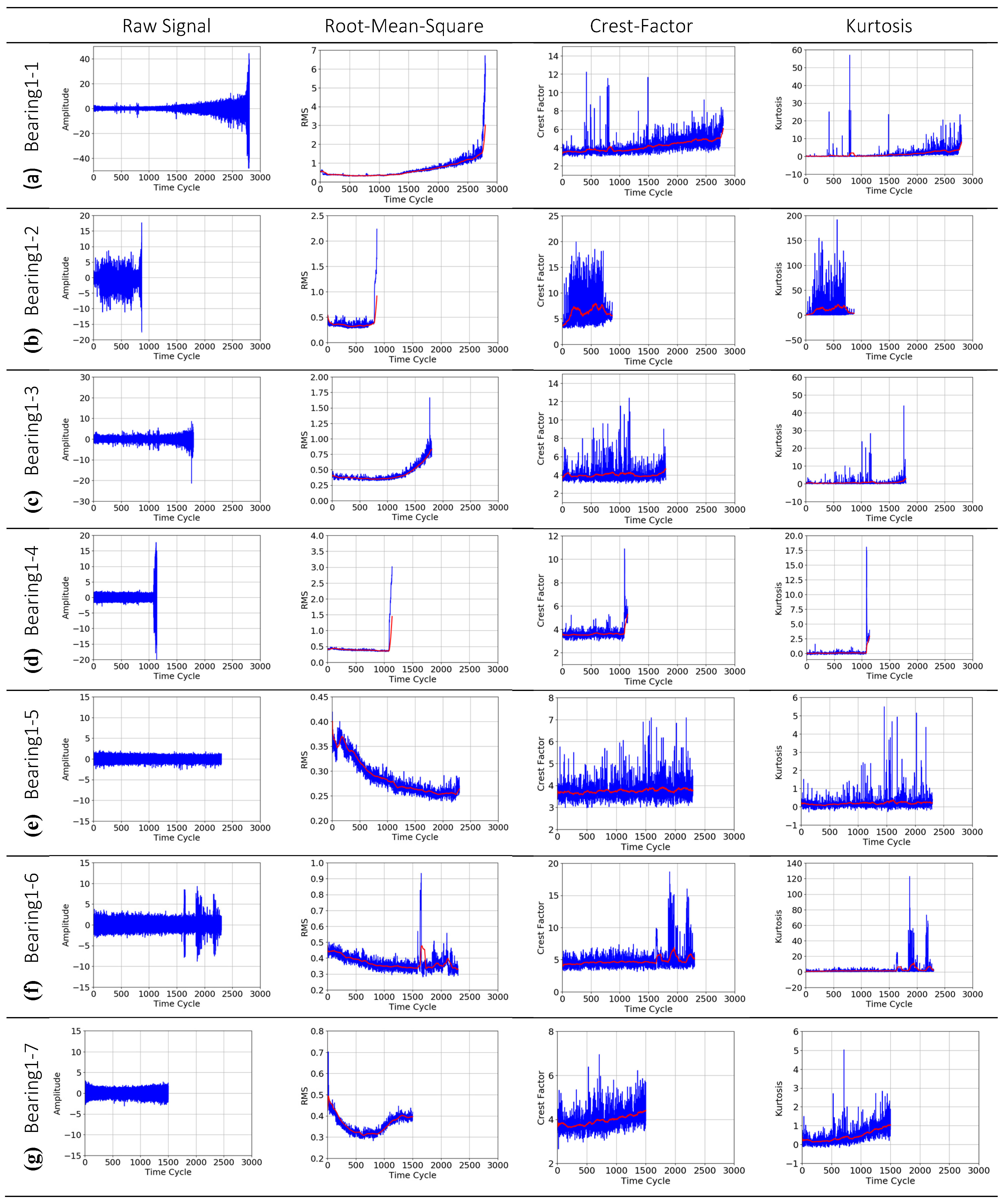
2. Problem Description

The open-access PRONOSTIA bearing datasets were produced by the FEMTO-ST Institute [15,16]. In the bearing experimental platform, namely PRONOSTIA, two accelerometers were mounted on the bearing housing to measure vibration in directions parallel and perpendicular to the gravity axis. Data were collected at 10 s intervals at a 25.6 kHz sampling rate for a 0.1 s duration. Hence, an observation contained 2560 sample points in each time cycle.

The bearing datasets were collected under three different operating conditions in variation of load and speed. For each operating condition (e.g., speed: 1800 rpm and load: 4000 N), only two sets of data from the entire run-to-failure experiments were provided. These are used as learning instances in this study to build the RUL estimation model. Partial data from run-to-failure experiments obtained by truncating the time series after a certain number of time cycles are also provided and used as test instances. In the 2012 PHM Prognostic Challenge [15,16], RUL was defined as the time span until the vibration amplitude exceeds 20 g.

Figure 1 shows vibration signals in the horizontal direction, i.e., perpendicular to gravity, under the operating condition I, i.e., speed of 1800 rpm and load of 4000 N. A total of seven datasets are provided including two learning instances labelled as Bearing1-1 and Bearing1-2, and five test instances labelled as Bearing1-3, 1-4, 1-5, 1-6, and 1-7. The two run-to-failure datasets show very different lifespans. A large variation in data length can be seen among the seven bearing instances (from 1 h to 7 h). The test bearing has 13 rolling elements with 3.5 mm diameter. Its inner race diameter is 22.1 mm and outer race diameter is 29.1 mm. The bearing has a contact angle of zero degrees.

For the 2012 PHM challenge, no information about the type of failure, e.g., fatigue spalling and its location or poor lubrication, was given. The data provider from the FEMTO-ST Institute has advised that theoretical models based on bearing characteristic frequencies were highly unlikely to be useful in identifying bearing fault types, because degradation of all bearing components may take place at the same time. In addition, theoretical reliability framework, e.g., L10 law, ball-pass-frequency-inner (BPFI), ball-pass-frequency-outer (BPFO) does not match the experimental observations very well [15].

There have been a variety of statistical measures that can be used to extract prognostic features from vibration signals, including Peak, Peak-to-Peak, Energy, Variance, Standard Deviation (SD), Root-Mean-Square, Entropy, Kurtosis, Skewness, Crest Factor, K-Factor, Impulse Factor, Margin Factor (i.e., Clearance Factor), Shape Factor (i.e., Form Factor, Wave Factor), and the trigonometric function based features SD-IHC and SD-IHS (i.e., SD of inverse hyperbolic cosine (IHC), SD of inverse hyperbolic sine (IHS)) [3,7]. For each time cycle containing a set of data points that are within the signal sampling duration, these statistical measures can be computed.

Some statistical parameters are reported to have the ability to indicate the severity of bearing faults [15]. For example, signal energy is generally proportional to the severity of bearing damage and hence parameters such as Root-Mean-Square and Peak-to-Peak should increase as faults progress. Other parameters, including the Crest Factor and the Impulse Factor, are sensitive to incipient faults and hence should increase as faults develop in the bearing but will fall back down as faults become widespread. Figure 1 shows the values and trends of Root-Mean-Square, Crest Factor, and Kurtosis for the 7 bearing instances under the operating condition of 1800 rpm and 4000 N. They were calculated for every time cycle. However, it is apparent that not a single parameter demonstrates consistent patterns across all 7 instances as bearing faults progress. Thus, it is difficult to derive the RUL estimation model based on these statistical parameters.

In addition, the PRONOSTIA data provider demonstrated that the evolution of the signal power spectrum density (PSD) shows monotonic increasing trend during bearing degradation for an ideal case such as Bearing1-1. However, they have also advised that, in most cases, the degradation appears suddenly and does not depict a slow monotonic behavior. In those cases, finding a prediction model is much more difficult based on PSD [15].

3. An Instance-Based Learning (IBL) Approach

In this section, we formulate the RUL estimation problem and present an overview of the proposed IBL approach. We then provide details of major components of the proposed approach, using the horizontal vibration signals of the 7 bearing instances under the operating condition I (i.e., 1800 rpm/4000 N) in the PRONOSTIA bearing datasets.

3.1. Formulation of the RUL Estimation Problem

Given a learning instance (denoted by superscript (l)) of the vibration signal, the run-to-failure degradation process can be represented by

$$\left\{\left(x_i^{\left(l\right)}, RU{L}_i^{\left(l\right)}\right)\right\} i=0, 1, 2, \dots ,M$$

(1)

where x_i^(l) represents the prognostic feature vectors of dimension K at time cycle i indexed from the beginning of bearing usage. M denotes the end of useful life.

$$x_i^{\left(l\right)}={\left(x_1, x_{2,},\dots , x_K\right)}_i^{\left(l\right)}$$

(2)

Features are extracted from raw signals at every time cycle. Recall that the PRONOSTIA datasets provide recordings of 0.1 s duration at intervals of every Δt = 10 s. In Equation (1), $RU{L}_i^{\left(l\right)}$ is the RUL at time cycle i. Hence:

$$RU{L}_i^{\left(l\right)}=M-i$$

(3)

For a test instance, the degradation process can be represented much the same way except we use superscript (p) to distinguish test from learning instances

$$\left\{\left(x_j^{\left(p\right)}, RU{L}_j^{\left(p\right)}\right)\right\} j=0, 1, 2, \dots ,N$$

(4)

with feature vectors represented by:

$$x_j^{\left(p\right)}={\left(x_1, x_{2,},\dots , x_K\right)}_j^{\left(p\right)}$$

(5)

In the above, index N denotes the last data recording. Obviously, $RU{L}_j^{\left(p\right)}$ is to be estimated and finding $RU{L}_N^{\left(p\right)}$ is the ultimate goal.

The key to the IBL approach lies in the selection of a learning instance from historical datasets, whose degradation process is deemed similar to the given test instance. Once a learning instance has been identified, the RUL problem can be solved by identifying the location of the current time cycle in the life cycle of the learning instance in order to determine the remaining useful life $RU{L}_N^{\left(p\right)}$.

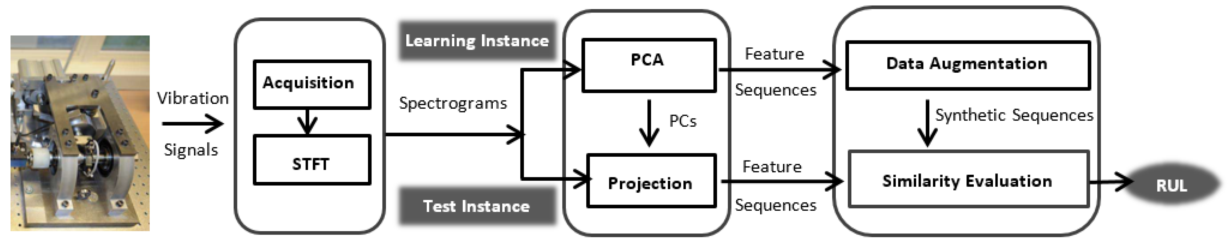
3.2. Overview of Methodology

As illustrated in Figure 2, the proposed IBL approach consists of three major components, namely, spectrogram generation, feature extraction, and RUL estimation:

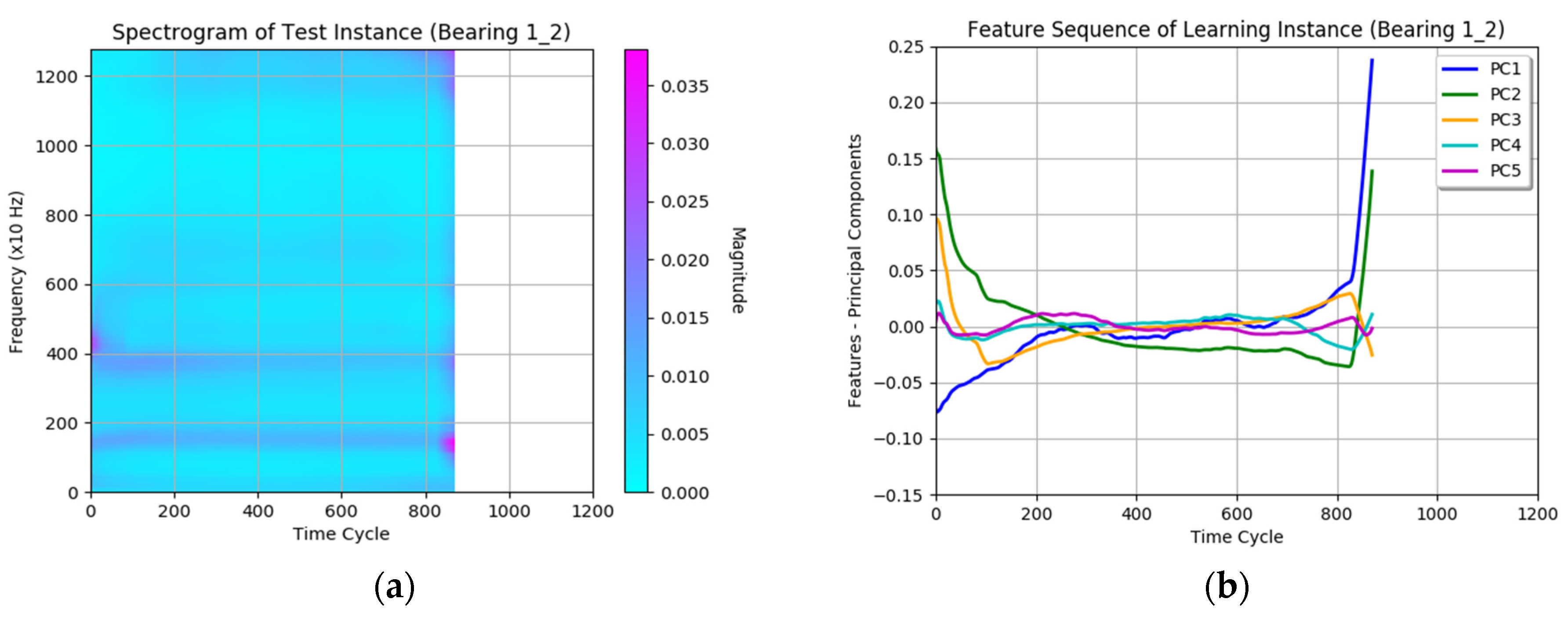
• Spectrogram generation applies the short-time-Fourier-transform (STFT) technique on the raw signals during each time cycle to generate frequency domain signals, so that spectrograms can be obtained for both learning and test instances.
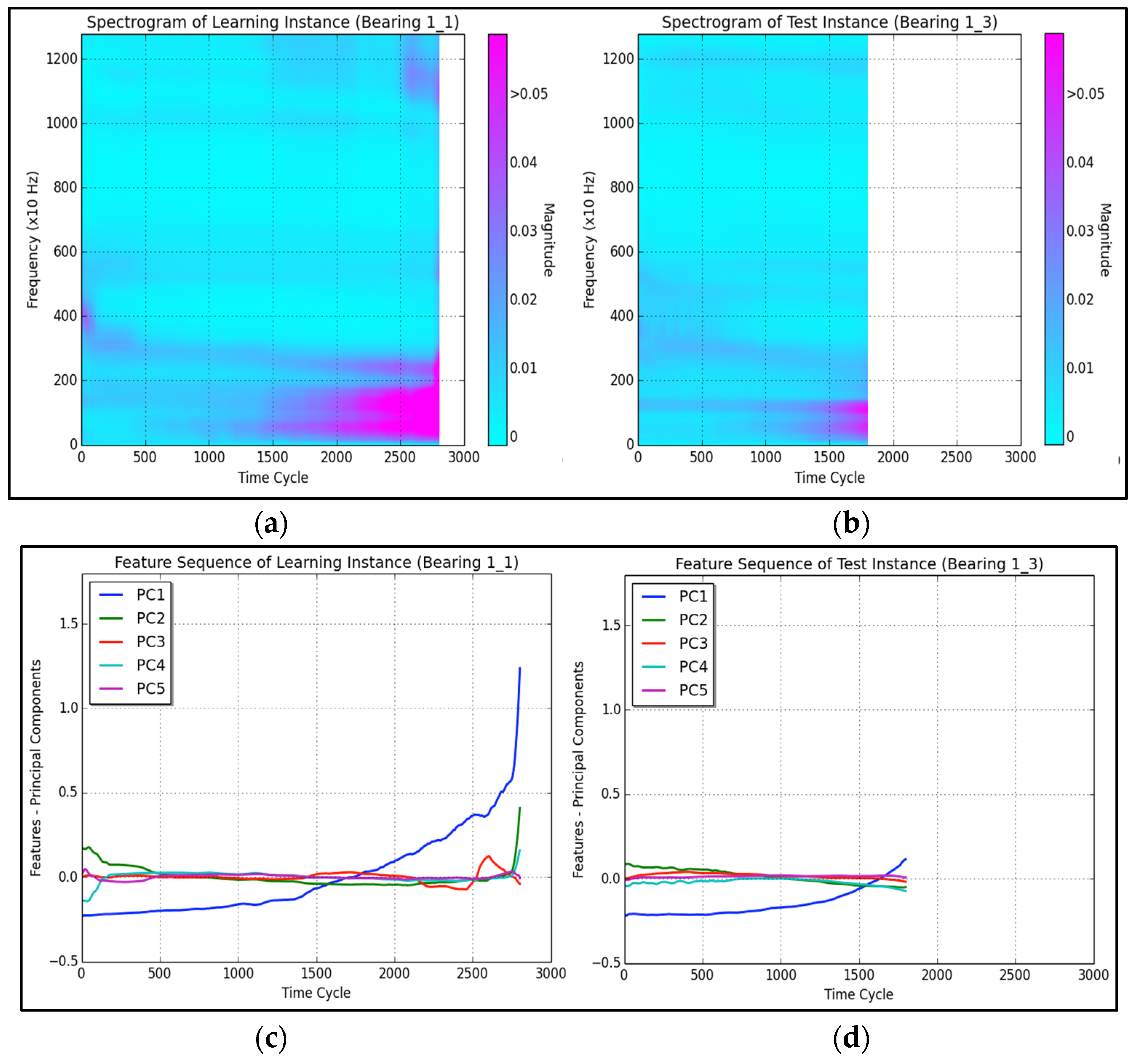
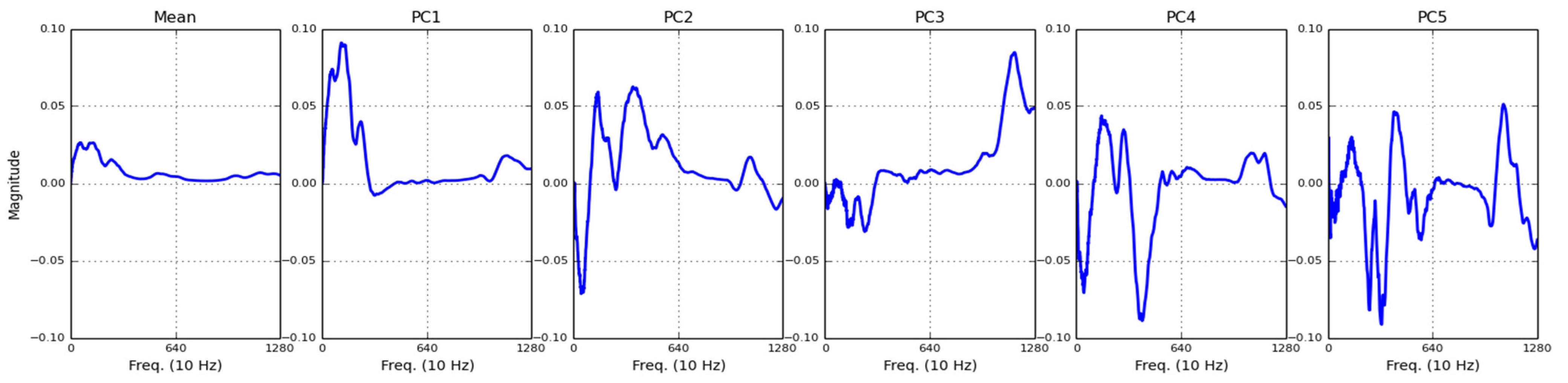
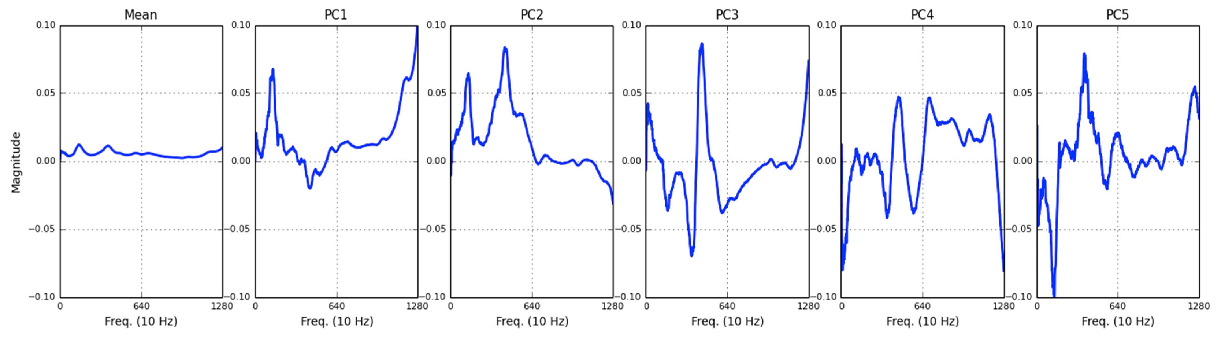
• Feature extraction is conducted using the principal component analysis (PCA) technique. The principal components (PCs) are calculated from the spectrogram of learning instances. Prognostic features are the coefficients of a spectrogram when projected onto the PCs.
• RUL estimation provides the RUL estimate for the test instance by identifying its similar prognostic feature sequences, which are generated synthetically from the learning instance using the data augmentation method.

3.3. Spectrogram Generation and Feature Extraction

In the PRONOSTIA datasets, data were collected every 10 s for a period of 0.1 s. In every time cycle of 0.1 s, 2560 data points were recorded, thus with a time resolution of 3.91 µs and frequency resolution of 10 Hz. Each spectrum obtained for each time cycle contains 1280 frequency components. In order to reduce noise effects, spectrograms are smoothed using moving averaging filters in both time and frequency directions. We chose 80 and 40 as the window sizes in time and frequency, respectively. Figure 3a,b show the spectrograms of Bearing1-1 as the learning instance and Bearing1-3 as the test instance.

For a learning instance, the spectrogram has 1280 frequency components at each of the M time steps so the PCA technique is utilized for dimension reduction. The PCA can reduce a larger number of features to the representative principal components using a linear transformation while maintaining most of the variability of the dataset [17]. In the proposed IBL approach, PCA is first applied to the spectrogram of the learning instance to generate a set of PCs (i.e., a set of eigenvectors). We chose the first five PCs to represent the bearing degradation states. In Figure 4, we show the mean and first five PCs of the learning instance Bearing1-1. They account for 91.27%, 5.13%, 1.48%, 0.14%, 0.03% of the spectrogram variability respectively, for a total of 99.86% of the data variability.

By projecting spectrograms onto the five major PCs generated above, the corresponding PC coefficients of both learning and test instances can be obtained. The spectrum at each time cycle i (or j) can be approximately represented by coefficients x_k,i (or x_k,j) on a total of 5 major principal components PC_k (k = 1, 2, 3, 4, 5) as shown in Figure 4.

$$Spectrum\left(i\right)={\displaystyle \sum }_{k=1}^5{x}_{k,i}·P{C}_k$$

(6)

These coefficients are considered as the prognostic features that are included in the prognostic feature vector x_i^(l) or x_j^(p) in Equations (2) and (5) to represent a bearing’s degradation state.

As a result, the five PC feature sequences can be obtained as illustrated in Figure 3c,d for Bearing1-1 and Bearing1-3, respectively. From these figures, it can be observed that the 1st PC mainly captures the variability of the learning instance data over time and also the test instance has a similar trend with respect to the 1st PC feature sequence. It is reasonable to associate machine health conditions with such variability in the bearing vibration data. Particularly, we can see that the 1st PC mainly reflects the variability of the vibration signal at two frequency ranges 0–3 kHz and 10–12 kHz, as shown in Figure 4.

The procedure is summarized as follows:

<Procedure–I: Spectrogram Generation and Feature Extraction>

1.

Spectrogram Generation

(1.a)

Generate spectrograms from raw vibration signals using the STFT.

(1.b)

Smooth the spectrogram generated from (1.a) using a moving average filter in frequency.

(1.c)

Smooth the spectrogram obtained in (1.b) using a moving average filter on time.

2.

Feature Extraction

(2.a)

Apply PCA to the spectrogram of the learning instance generated in (1.c) and select the first five eigenvectors as the principal components for dimension reduction.

(2.b)

Project the spectrograms onto the PC obtained in (2.a). The coefficients of projection are the prognostic features.

3.4. RUL Estimation

The step of RUL estimation is approached with three components, namely, data augmentation, similarity evaluation, and estimate ensemble. Details are provided below.

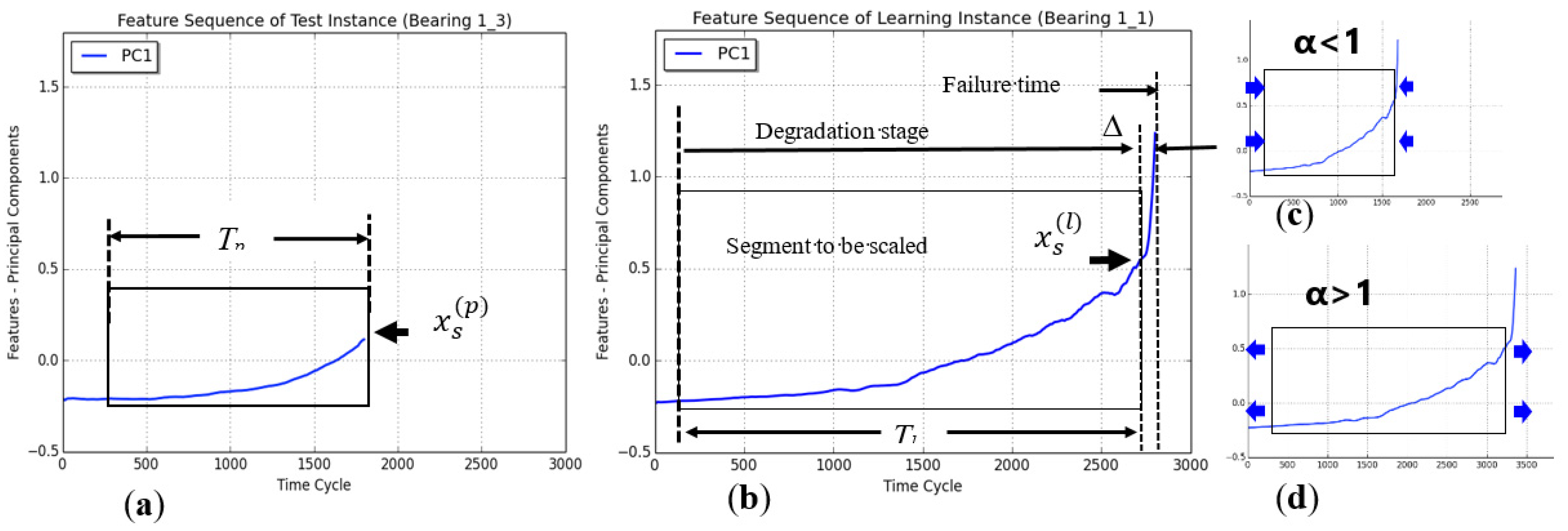
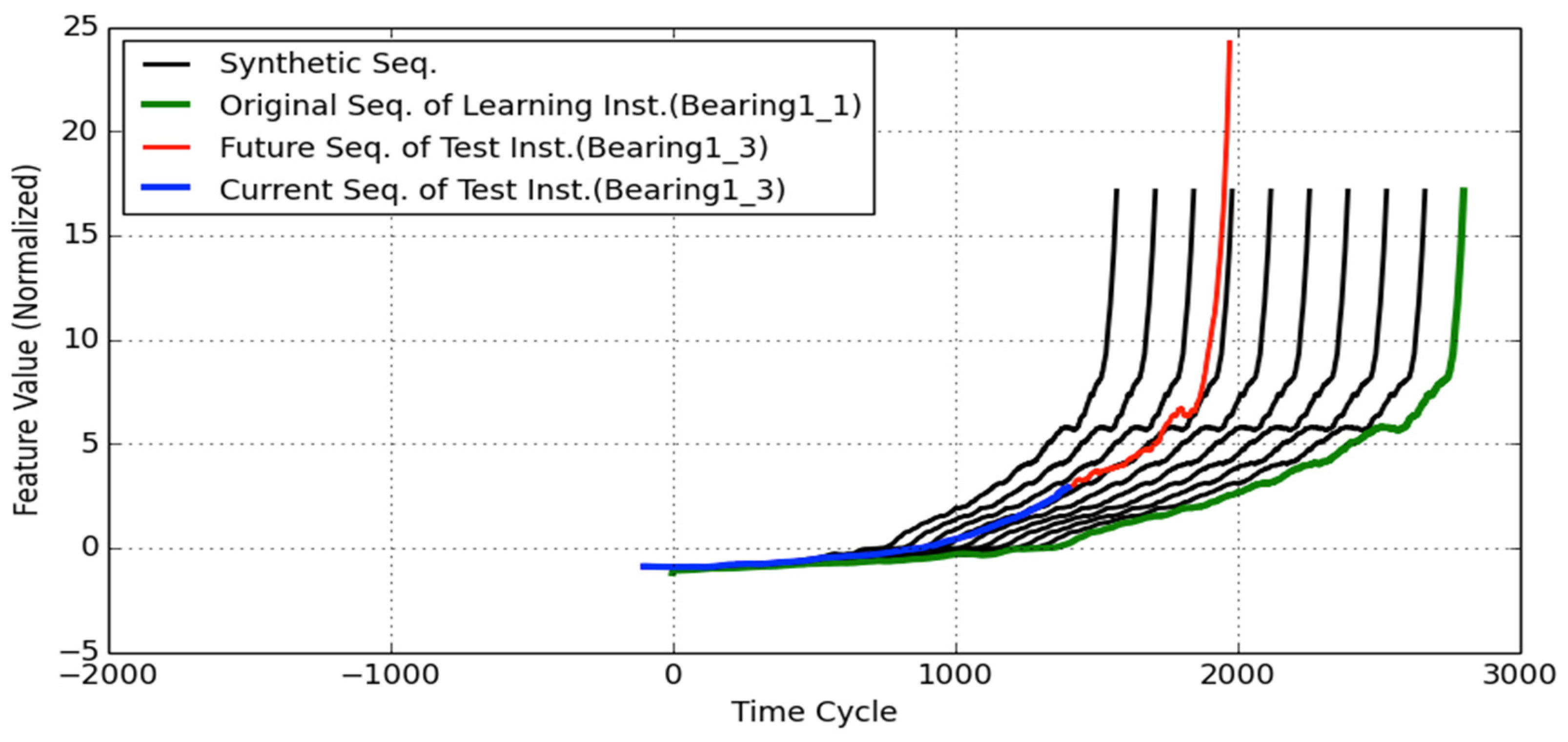
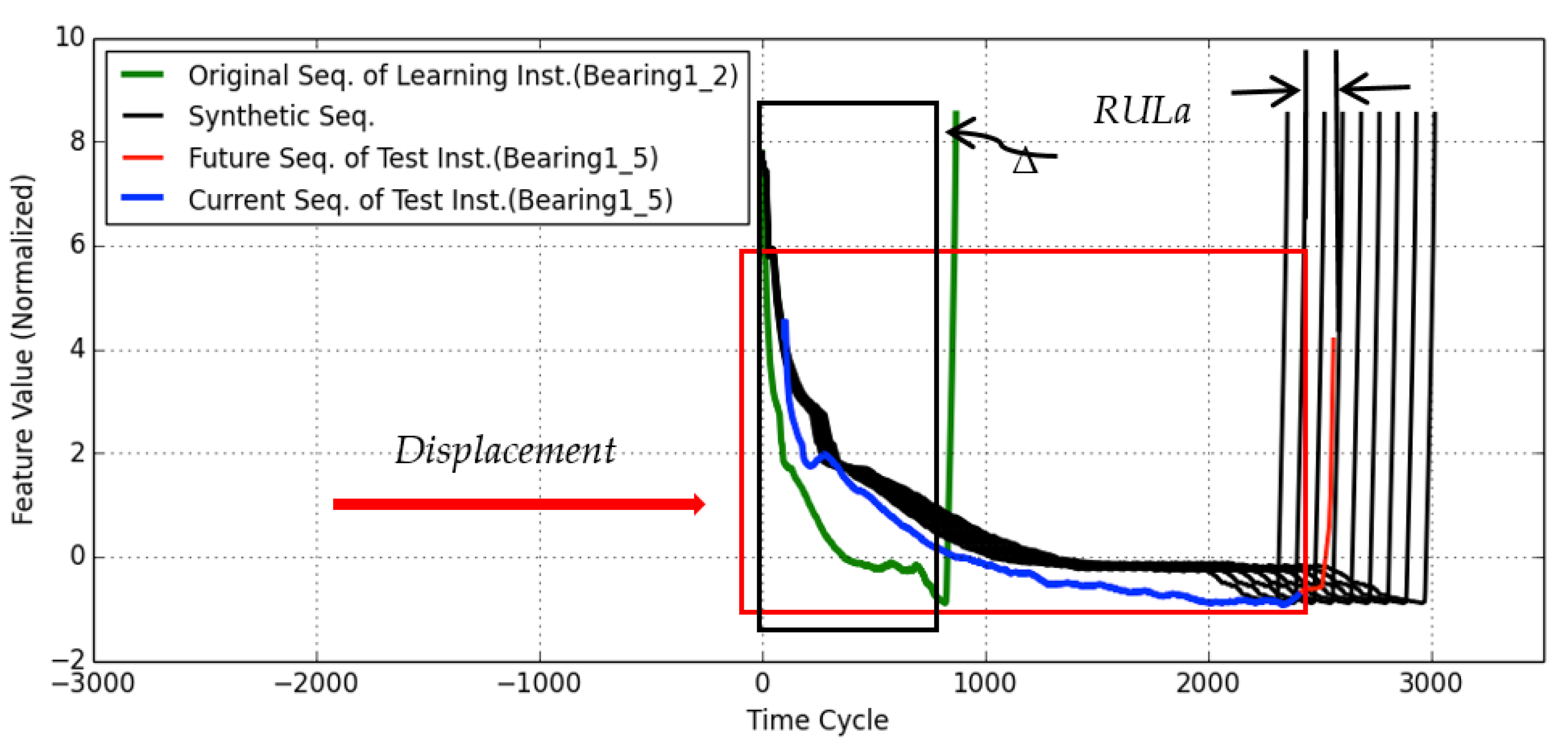
3.4.1. Data Augmentation

In machine learning applications, a data augmentation strategy is often used to generate additional learning data by modifying the historical samples [18,19,20]. By increasing the learning datasets, classification models can be trained to be more robust and generalized without over-fitting. For example, in image analysis, learning samples may be acquired under a limited set of conditions. However, classification may need to be applied to images under conditions beyond that of the learning samples, such as different orientation, location, scale, brightness, etc. These situations can be accounted for by training the classification model with additional image samples, which may be generated by synthetically modifying existing samples through translation, rotation, scaling, and illumination. Augmenting the learning datasets can result in a trained classification model to be more robust and generalized with-out over-fitting. Taking a similar approach, we propose a segment scaling method in order to generate synthetic feature sequences by modifying the learning instance in the IBL approach for bearing RUL estimation.

We take the learning instance Bearing1-1 as an example. Figure 5b shows the 1st PC feature sequence over time. Based on the magnitude trend of the feature curve, three typical stages within the lifespan of the learning instance can be observed: (i) normal stage where no obvious degradation occurs, the magnitude remains nearly constant; (ii) degradation stage where a gradually changing trend is clear; (iii) close-to-failure stage where the bearing is close to failure as signaled by steep or abrupt changes in the feature curve. The close-to-failure stage may last a short period, while the degradation stage can last quite long.

Figure 5a shows the 1st PC feature sequence of the test instance. If we can determine the equivalent location of the test instance relative to the lifespan of the learning instance, we can estimate the RUL of the test instance. As illustrated in Figure 5a, the proposed segment scaling method starts by identifying a defect-degradation segment in the first PC feature sequence of the test instance Bearing1-3. The specified segment for the test instance begins on entering the degradation stage until the current time cycle. Correspondingly, specify a degradation segment of length T_l within the feature sequence of the learning instance. The learning degradation segment should present similar trending as the test segment. For the learning instance, the specified segment also begins on entering the degradation stage until ending the entire degradation stage. Understandably, the learning degradation segment should encompass the test segment in magnitude so that it is possible to determine the relative location of the test case degradation. Hence, the following condition Equation (7) should be satisfied for the specified test and learning segments.

$$\{\begin{array}{c}{x}_s^{\left(p\right)}\le x_s^{\left(l\right)}, for increasing trend\\ x_s^{\left(p\right)}\ge x_s^{\left(l\right)}, for decreasing trend\end{array}$$

(7)

where $x_s^{\left(p\right)}$ and $x_s^{\left(l\right)}$ are prognostic feature values of the test and learning instances at the ending times of their respective segments, as illustrated in Figure 5a,b.

The learning degradation segment is then stretched (α > 1) or shrunk (α < 1) in length with different scaling factor α, as illustrated Figure 5b–d. By scaling, multiple segments representing different prognostic feature sequences from the given learning instance can be generated. The heuristics are based on the following assumptions [21,22]: (a) The same type of bearing faults may progress in different degradation rates due to different conditions including fault initial status, material heterogeneity, and lubrication condition, even though under the same loading and rotation conditions; (b) As the segments within the close-to-failure stage and normal stage are not used in the similarity comparisons between the test and learning instances, the segment scaling method is only applied on the learning degradation segment; (c) The time of the close-to-failure stage, Δ as indicated in Figure 5b, is approximately considered as a constant in all synthetic learning sequences, as this last stage of bearing life is usually relatively shorter than its gradual degradation stage.

This segment scaling method is implemented by resampling with a linear or spline interpolation function [23]. At first, the interpolation function is constructed to approximate the specified segment of the learning instance.

$$x_i=S\left(i\right) i=0, 1, 2, \dots , T_l$$

(8)

where x_i is the interpolated feature value at the time cycle of index i. Then, a new feature sequence in the scaled length αT_l is generated by re-interpolating the linear or spline function as illustrated in Figure 5c,d.

$$x_i=S\left(i/\alpha \right) i=0,1, 2, \dots , \alpha T_l$$

(9)

where x_i is the interpolated feature value at the time cycle of index i on the synthetic sequence, and the scaled length αT_l needs to be rounded if it is not an integer. At last, the normal segment, the synthetic degradation segment, and the close-to-failure segment are concatenated sequentially to generate the entire synthetic feature sequence. Accordingly, multiple synthetic learning feature sequences can be generated with different scaling factors.

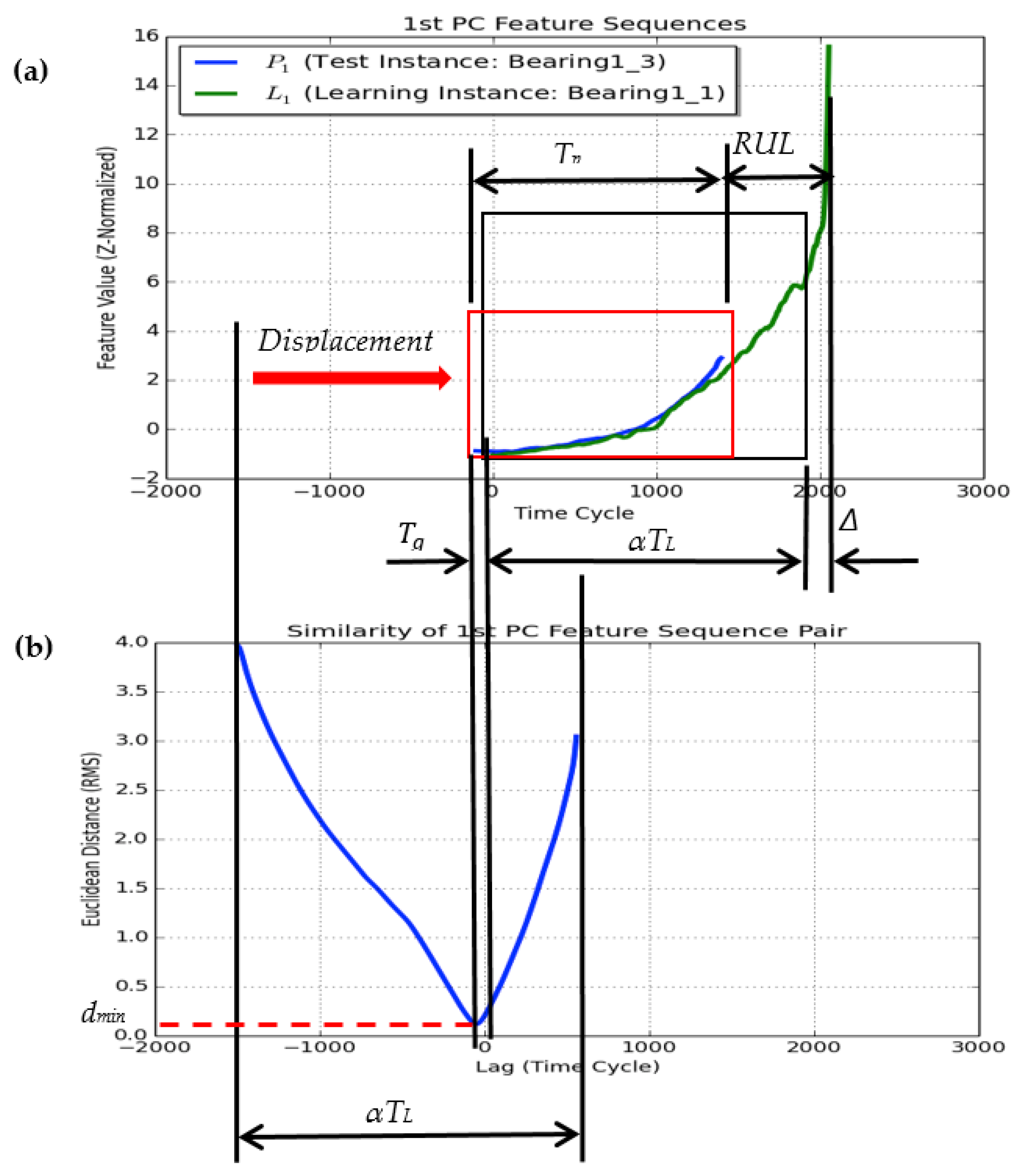
3.4.2. Similarity Evaluation

If we can determine “a segment” in the learning instance feature sequence that is “similar” to that of the test instance, we can conclude its RUL without much difficulty. This segment may be original or synthetic as described above. We now describe how to assess similarity. In this study, we use the root mean squared (RMS) difference measure to evaluate similarity between the test and learning instances, as described below.

Figure 6 illustrates the similarity matching by using the 1st PC, that is, k = 1. In particular, it depicts the prognostic feature segment of the test instance (e.g., Bearing1-3), P_k, and one of the synthetic feature sequences (e.g., α = 0.75) of the learning instance (e.g., Bearing1-1), L_k.

$$P_k=\left(x_{k,0}^{\left(p\right)},x_{k,1}^{\left(p\right)},\dots x_{k,j}^{\left(p\right)},\dots x_{k,T_p}^{\left(p\right)}\right)$$

(10)

$$L_k=\left(x_{k,0}^{\left(l\right)},x_{k,1}^{\left(l\right)},\dots x_{k,i}^{\left(l\right)},\dots x_{k,\alpha T_l}^{\left(l\right)}\right)$$

(11)

By displacing P_k along the time axis, the similarity measure method computes the difference between L_k and each shifted P_k in the form of RMS using the following function of time displacement T_g:

$$d\left(P_k,L_k,T_g\right)=\{\begin{array}{c}\sqrt{\frac{1}{T_P}{\displaystyle {\displaystyle \sum }_{i=0}^{T_P}}{\left(x_{k,i}^{\left(p\right)}-x_{k,i+T_g}^{\left(l\right)}\right)}^2} \left(T_g\ge 0\right) \\ \sqrt{\frac{1}{\left(T_p+T_g\right)}{\displaystyle {\displaystyle \sum }_{i=0}^{\left(T_p+T_g\right)}}{\left(x_{k,i-T_g}^{\left(p\right)}-x_{k,i}^{\left(l\right)}\right)}^2} (T_g<0)\end{array}$$

(12)

Recall that T_p, and αT_l, are the lengths of the two feature segments being compared. T_g is in the range of [−T_p, αT_l, − T_p]. The best matching between the two segments is indicated by a minimum value of similarity measure d_min. Figure 6b shows the similarity measure $d\left(P_k,L_k,T_g\right)$ for the given segments of comparison as a function of displacement $T_g.$ At d_min, the displacement is denoted as $T_{g,min}$. For each given synthetic feature sequence (e.g., α = 0.75), we identify the d_min(α) and the RUL measured in time cycles then can be calculated by:

$$RUL \left(\alpha \right)=\alpha T_l-\left(T_p+T_{g, min}\right)+\Delta$$

(13)

In the above equation, Δ as indicated in Figure 6a, is constant for all synthetic feature sequences because it is excluded from scaling. In the example shown in Figure 6, the prognostic segments are chosen between 300- and 1800-time cycles from the test instance and between 20- and 2750-time cycles from the learning instance. Therefore, T_p = 1500, T_l = 2730. The learning instance Bearing1-1 is recorded as failing at 2785 cycles, hence Δ = 53. At the best matching, $T_{g, min}=$−34, α = 0.75. Thus, RUL (0.75) = 0.75 × 2730 − (1500 − 34) + 53 = 635 (time cycles).

Note that in the above computation each comparison pair of feature sequences, L_k and P_k, are normalized with the mean $\mu$ and standard deviation $\sigma$ of the feature segment P_k, using Equations (14) and (15), respectively. In this way, the similarity metrics d_min for all different pairs of test and learning sequences are in the consistent measurement scale [0, 1], where smaller d_min indicates a more similar pair of comparison sequences.

$$\left(L_k-\mu \left(P_k\right)\right)/\sigma \left(P_k\right)$$

(14)

$$\left(P_k-\mu \left(P_k\right)\right)/\sigma \left(P_k\right)$$

(15)

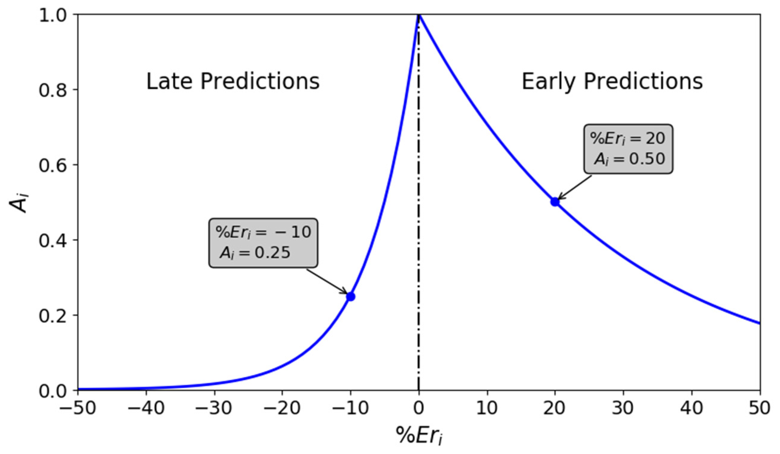
3.4.3. Estimate Ensemble

Once synthetic data are generated, we can try to find the best match between the test instance and the learning instance by the similarity measures of all real and synthetic data. As the synthetic learning sequences are generated in the discrete way (with a set of scaling factors), the estimation result may be biased from the actual RUL if it is only based on one synthetic sequence. Hence, we propose an ensemble method based on multiple synthetic learning sequences to achieve the best out-come of assessing RUL.

As illustrated in Figure 7, multiple synthetic feature sequences are generated from the original feature sequence of the learning instance (e.g., Bearing1-1) with different scaling factor α. From each synthetic sequence, an RUL estimate, RUL(α), for the test instance (e.g., Bearing1-3) can be obtained with the corresponding minimum similarity measure d_min(α). A scaling factor α* for the best similarity matching sequence can be identified from all learning sequences including the original and synthetic ones. After that, the final RUL estimation can be aggregated from the best matching sequence and the multiple synthetic sequences, whose scaling factors are evenly distributed on both sides of α*, for example, two sequences with α > α* and two sequences with α < α*, as shown in Figure 7. The formula for computing the ensemble RUL estimate is defined as Equation (16). In the averaging formula of the ensemble method over M number of the selected sequences, each RUL estimate is weighted by its corresponding similarity measure, d_min.

$$RU{L}_e=\raisebox{1ex}{${\displaystyle {\sum }_{m=1}^M}\left(RUL\left({\alpha }_m\right)/d_{min}\left({\alpha }_m\right)\right)$}\!\left/ \!\raisebox{-1ex}{${\displaystyle {\sum }_{m=1}^M}\left(1/d_{min}\left({\alpha }_m\right)\right)$}\right.$$

(16)

In this example as illustrated in Figure 7, nine synthetic sequences are generated from the original feature sequence of Bearing1-1, with the scaling factor α of 0.55, 0.60, 0.65, 0.70, 0.75, 0.80, 0.85, 0.90, and 0.95, respectively.

Table 1. Similarity evaluation for RUL estimation between Beaing1-3 and Bearing1-2.

α	0.55	0.60	0.65	0.70	0.75	0.80	0.85	0.90	0.95
dmin(α)	0.2384	0.1857	0.1434	0.1190	0.1137	0.1225	0.1400	0.1621	0.1814
RUL(α)	423	473	523	578	635	693	756	823	887

presents the results of a similarity evaluation between the nine synthetic sequences and the selected segment in the range of [300, 1800] (time cycles) of Bearing1-3. The best similarity matching sequence can be identified as α = 0.75. Based on the seven selected synthetic feature sequences with α = 0.60, 0.65, 0.70, 0.75, 0.80, 0.85, and 0.90, the ensemble RUL estimate, $RU{L}_e$, can be computed as 642 (time cycles) using Equation (18). The actual RUL at the last time cycle 1800 (i.e., the length of future sequence) of Bearing1-3 is $RU{L}_a$ = 573 (time cycles). Thus, our proposed IBL approach can achieve a good performance with the relative error $E_r$ = −12.07%, which is calculated using the formula Equation (17).

$$E_r=\left(RU{L}_a-RU{L}_e\right)/RU{L}_a$$

(17)

In summary, the procedure for the RUL estimation method with data augmentation is described as follows:

<Procedure–II: Data Augmentation and RUL Estimation>

1.

Data Augmentation

(1.a)

Specify the pair of comparison feature segments within the test instance and learning instance, P_k and L_k (i.e., α = 1.0).

(1.b)

Generate multiple synthetic sequences L_k (i.e., α > 1.0 or α < 1.0) from the original one using the segment scaling method described in Section 3.4.1.

2.

Similarity Evaluation

(2.a)

Compute the similarity measure as expressed in Equation (12) between the P_k and each sequence L_k using the similarity evaluation method as described in Section 3.4.2

(2.b)

Identify the minimum similarity measure d_min and the corresponding displacement $T_g$ with respect to P_k.

(2.c)

Repeat the steps (2.a) and (2.b) for each pair of sequences P_k and L_k.

3.

Estimate Ensemble

(3.a)

Identify the best similarity matching pair of sequences from all the similarity evaluation results.

(3.b)

Select several learning sequences (e.g., 4 sequences in this study) around the best similarity matching sequence identified in (3.a).

(3.c)

Compute the final RUL estimate using Equations (16) and (17) based on the results obtained from the best matching sequence in (3.a) and the sequences selected in (3.b).

4. Results and Comparison

In the previous section, we described the proposed IBL approach step by step with the example of the test instance Bearing1-3 and the learning instance Bearing1-1 in the PRONOSTIA bearing datasets. The RUL estimation results for the four other test bearings under the operating condition I (1800 rpm and 4000 N), including Bearings 1-4, 1-5, 1-6, and 1-7, are discussed in this section.

4.1. RUL Estimation for Test Instance Bearings

The spectrogram and its corresponding PC feature sequences for the learning instance Bearing1-2 are shown in Figure 8a,b, respectively. In Figure 9, we show the first five PCs of the learning instance Bearing1-2. They each account for data variability of 49.78%, 37.45%, 9.24%, 1.71%, 0.98%, respectively. As shown in Figure 9, we can observe that the 1st PC mainly reflects the variability of the vibration signal at two frequency ranges 0–3 kHz and 10–12 kHz, the 2nd PC at two frequency ranges 0–3 kHz and 3–5 kHz, and so on.

Recall that the first five PC sequences of Bearing1-1 have been illustrated in Figure 4 in the previous Section 3.3. For comparison,

Table 2. Accounts for variability of principal components of learning instances.

	PC1	PC2	PC3	PC4	PC5
Bearing1-1	91.27%	5.13%	1.48%	0.14%	0.03%
Bearing1-2	49.78%	37.45%	9.24%	1.71%	0.98%

summarizes the PCs for data variability with respect to Bearing1-1 and Bearing1-2.

Applying the proposed IBL approach to the bearing datasets, we compare the five PC feature sequences between each pair of a test instance and the augmented feature sequences of the learning instance. The best similarity matching sequence pair can be identified from the test instance vs. each learning instance. It should be noted that we only present the best matching sequence pair and the corresponding RUL estimate results for each test instance here.

As a result, the 2nd PC feature sequences were chosen for test instances Bearing1-5, 1-6, and 1-7 paired with the learning instance Bearing1-2. The 1st PC feature sequences are used for Bearing1-4 paired with the learning instance Bearing1-2. Figure 10 shows the five PC feature sequences of the test instances Bearings 1-4, 1-5, 1-6, and 1-7, which are generated by projecting their spectrograms on the PCs of learning instance Bearing1-2.

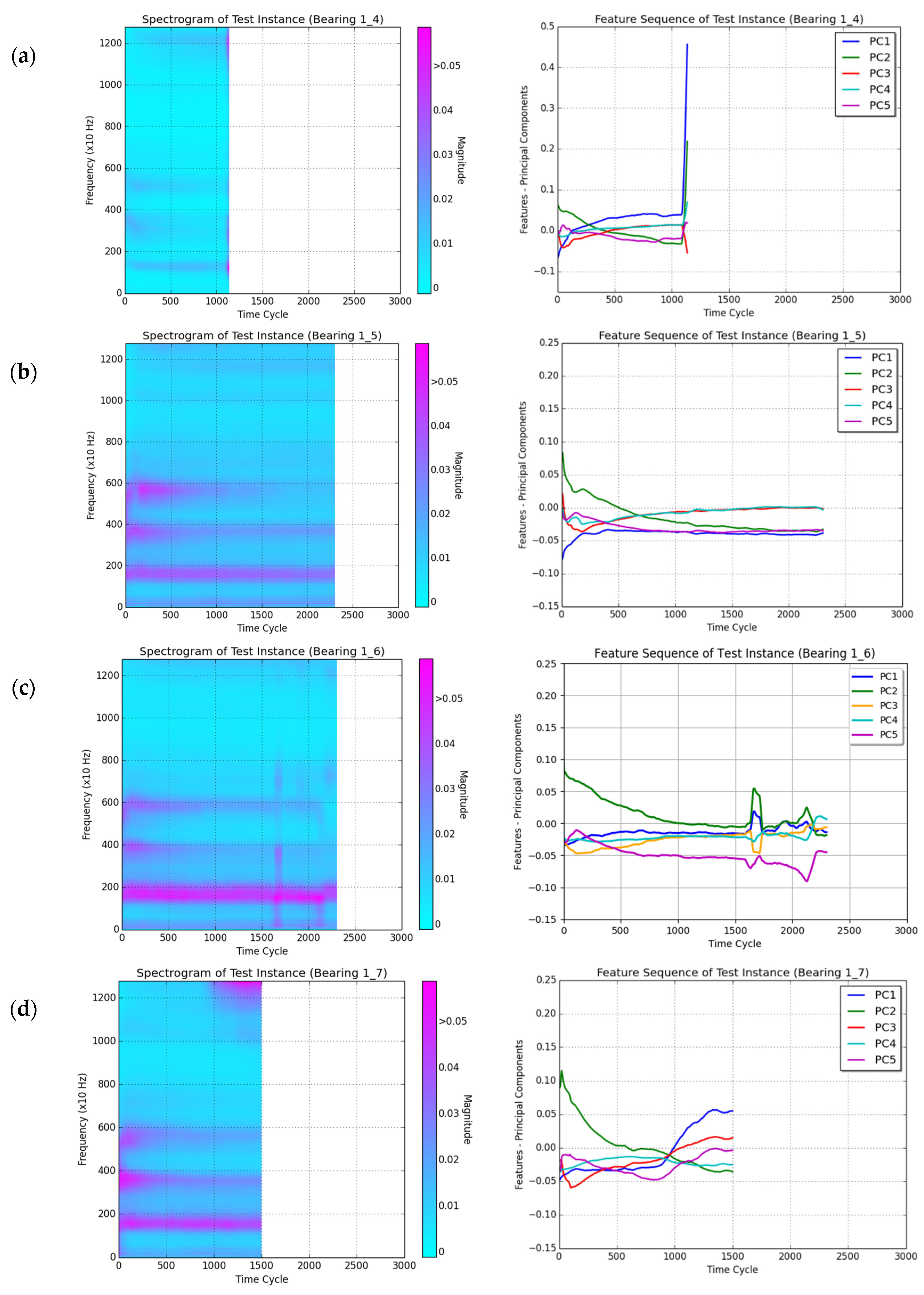
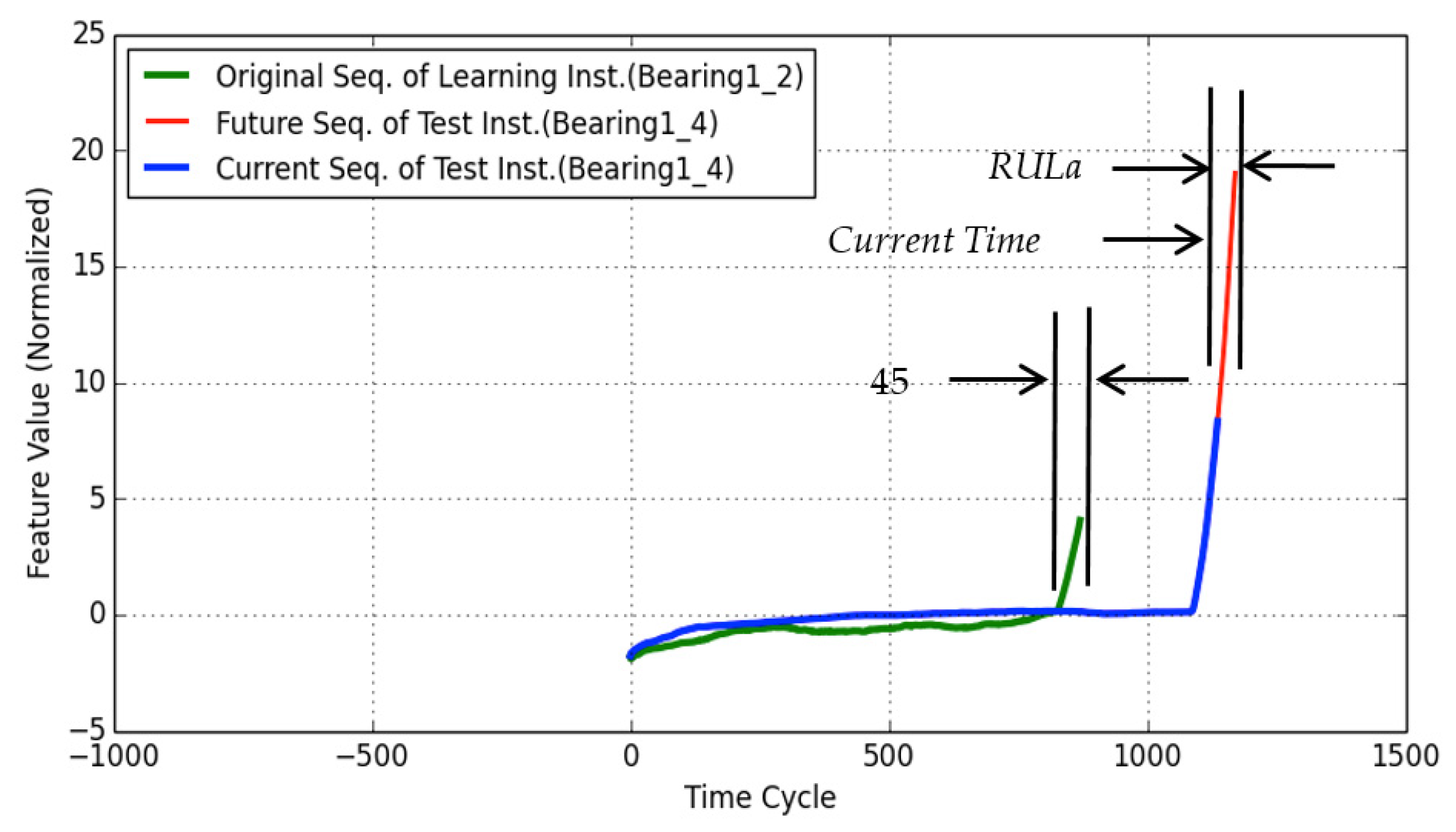
4.1.1. RUL Estimation for Test Instance Bearing1-4

Using Bearing1-2 as the learning instance, the pair of the 1st PC sequences with similar trends is compared to estimate the RUL for the test instance Bearing1-4. As illustrated in Figure 11, Bearing1-4 has passed its degradation stage and entered its close-to-failure stage at time cycle 1039 and records are given up to cycle 1137. Therefore, the usage of Bearing1-4 can be estimated pessimistically, and the RUL is estimated as 0 at time cycle 1137. On the other hand, the RUL of Bearing1-4 can also be optimistically estimated as the duration of close-to-failure stage of Bearing1-2, which is known as 45-time cycles from the turning point. Averaging the pessimistic and optimistic estimates, we conclude the final RUL estimate as $RU{L}_e$ = 23 (time cycles). As the actual RUL of Bearing1-4 is known as $RU{L}_a$ = 34 (time cycles), the estimation has the relative error $E_r$ = 32.4%.

4.1.2. RUL Estimation for Test Instance Bearing1-5

Based on the specified segment of the range [0, 825] (time cycles) within the 2nd PC feature sequence of the learning instance Bearing1-2, the nine synthetic feature sequences are generated with the scaling factor α of 2.80, 2.90, 3.00, 3.10, 3.20, 3.30, 3.40, 3.50, and 3.60, as shown in Figure 12. The duration Δ is equal to 45 (time cycles) in this case.

Table 3. Similarity evaluation for RUL estimation of Bearing1-5 using Bearing1-2.

α	2.80	2.90	3.00	3.10	3.20	3.30	3.40	3.50	3.60
dmin(α)	0.8149	0.4430	0.3562	0.3527	0.3750	0.3967	0.4166	0.4347	0.4495
RUL(α)	46	46	46	70	141	211	284	355	430

presents the results of similarity evaluation of synthetic sequences and the selected segment in the range of [0, 2303] (time cycles) of Bearing1-5. Based on the seven synthetic sequences of α = 2.90, 3.00, 3.10, 3.20, 3.30, 3.40, and 3.50, the final RUL estimate of Bearing1-5 can be computed as $RU{L}_e$ = 160 (time cycles) using the proposed ensemble method. As the actual RUL of Bearing1-5 is known as $RU{L}_a$= 161 (time cycles), the relative error of estimation is calculated as $E_r$ = 0.92%.

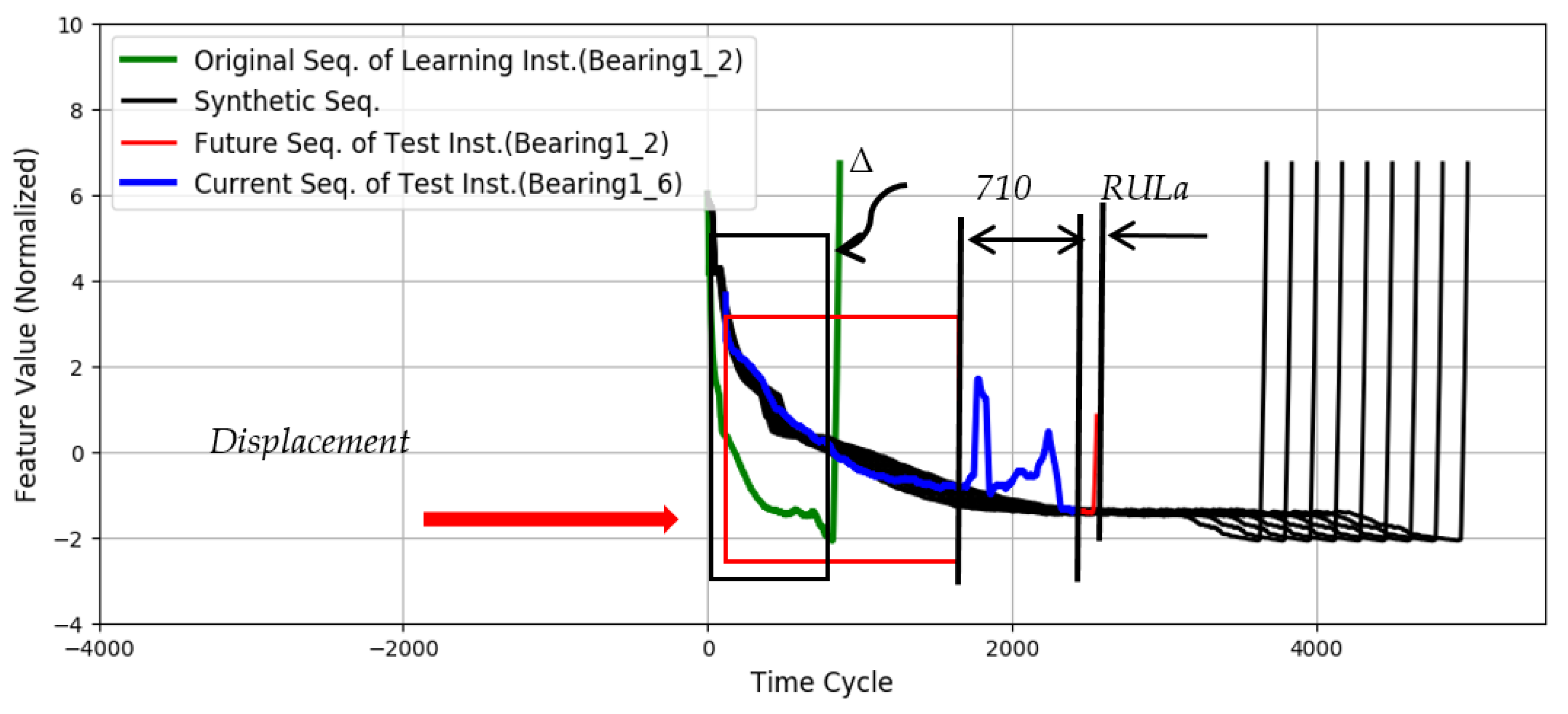
4.1.3. RUL Estimation for Test Instance Bearing1-6

The similarity evaluation for RUL estimation was made based on the pair of 2nd PC feature sequences between the test instance Bearing1-6 and the learning instance Bearing1-2. Initially, we specify the comparing segment as the monotonic segment in the range of [0, 1590] (time cycles) within the degradation stage of Bearing1-6. Using Bearing1-2, the segment of [0, 825] (time cycles) is specified to generate nine synthetic sequences with scaling factors of 3.40, 3.60, 3.80, 4.00, 4.20, 4.40, 4.60, 4.80, and 5.00, as shown in Figure 13. The duration Δ is equal to 45 (time cycles) in this case.

Table 4. Similarity evaluation for RUL estimation of Bearing1-6 using Bearing1-2.

α	3.40	3.60	3.80	4.00	4.20	4.40	4.60	4.80	5.00
dmin(α)	0.2689	0.2371	0.2145	0.2009	0.1963	0.2000	0.2109	0.2264	0.2444
RUL(α)	2031	2187	2342	2497	2652	2806	2959	3111	3263

presents the results of similarity evaluation for the RUL estimation. Based on the seven synthetic sequences of α = 3.60, 3.80, 4.00, 4.20, 4.40, 4.60, and 4.80, the final RUL estimate is computed as 2654 (time cycles) when the degradation process reached the time cycle 1590. As the degradation process has lasted 710-time cycles from the time cycle 1590 to the current time cycles 2300, thus $RU{L}_e$ = 2654 − 710 = 1944 (time cycles).

However, from the 2nd PC feature sequence, we can observe that sudden and abrupt interruptions occurred during the range of [1590, 2300] (time cycles) of the test instance. Thus, we may consider that the degradation process has entered the close-to-failure stage after the time cycle 1590. Reasonably, the RUL of Bearing1-6 can be estimated as $RU{L}_e$ = Δ = 45 (time cycles) at the last time cycle 2300. As the actual RUL is known as $RU{L}_a$ = 146 (time cycles), the relative error of estimation can be calculated as $E_r$ = 69.2%.

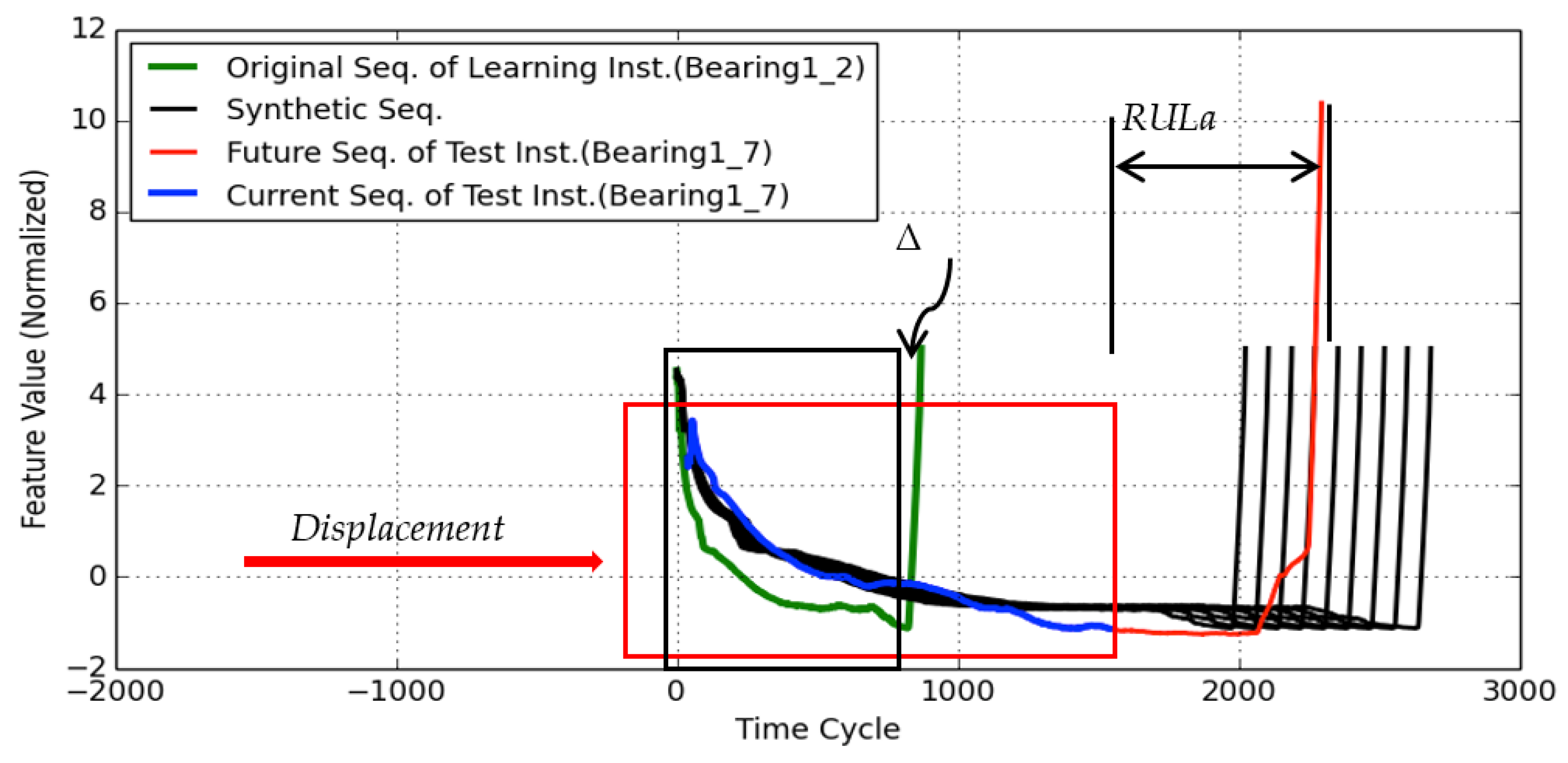
4.1.4. RUL Estimation for Test Instance Bearing1-7

The similarity evaluation for the test instance Bearing1-7 is performed based on the 2nd PC feature sequence using Bearing1-2 as the learning instance. From the segment of [0, 825] (time cycles) of Bearing1-2, the nine synthetic feature sequences are generated with the scaling factor α = 2.40, 2.50, 2.60, 2.70, 2.80, 2.90, 3.00, 3.10, and 3.20, as shown in Figure 14. The duration Δ is equal to 45 (time cycles).

Table 5. Similarity evaluation for RUL estimation of Beaing1-7 using Bearing1-2.

α	2.40	2.50	2.60	2.70	2.80	2.90	3.00	3.10	3.20
dmin(α)	0.2863	0.2741	0.2634	0.2537	0.2504	0.2517	0.2569	0.2644	0.2734
RUL(α)	481	581	661	740	819	908	977	1056	1135

presents the results of similarity evaluation between each synthetic sequence and the degradation segment of [0, 1500] (time cycles) of Bearing1-7. Selecting the seven synthetic sequences of α = 2.50, 2.60, 2.70, 2.80, 2.90, 3.00, and 3.10, the final RUL estimate can be computed as $RU{L}_e$ = 822 (time cycles) using the proposed ensemble method. As the actual RUL of Bearing1-7 is known as $RU{L}_a$ = 757 (time cycles), the relative error of estimation can be calculated as $E_r$ = −8.61%.

4.1.5. Summary of Results and Discussions

In the IEEE PHM 2012 Prognostic Challenge, a scoring function was used to evaluate the RUL estimation results as follows [15]. Based on the relative error Er obtained using Equation (17), the score of RUL estimation for each test bearing is defined as:

$$A=\{\begin{array}{c} ex{p}^{-ln\left(0.5\right)·\left(100·Er/5\right)} if Er\le 0\\ ex{p}^{+ln\left(0.5\right)·\left(100·Er/20\right)} if Er>0\end{array}$$

(18)

This scoring function can penalize both underestimates and overestimates such that (i) the perfect estimate corresponding to a perfect score of 1 (i.e., Er = 0), (ii) score deduction is given to estimates that are shorter than the actual bearing RUL (i.e., Er > 0), and (iii) a more severe score deduction is given to estimates that exceed the actual bearing RUL (i.e., Er < 0). Figure 15 depicts the scoring function. The overall estimation score averages the scores for N test bearings.

$$Score=\frac{1}{N}{{\displaystyle \sum }}_{i=1}^N{A}_i$$

(19)

The RUL estimation results for Bearing1-3, 4, 5, 6, and 7 (under the operating condition I) are summarized in

Table 6. Summary of RUL estimation results for Bearing1-3, 1-4, 1-5, 1-6, and 1-7.

Test Instance (Bearing)	1-3	1-4	1-5	1-6	1-7
Learning Instance (Bearing)	1-1	1-2	1-2	1-2	1-2
Comparing PC Feature No.	1st	1st	2rd	2rd	2rd
Similarity (dmin)	0.1137	-	0.3750	0.1963	0.2504
Last Time (time cycles)	1800	1137	2303	2300	1500
$RU{L}_a$ (time cycles)	573	34	161	146	757
$RU{L}_e$ (time cycles)	642	23	160	45	822
Relative Error	−12.1%	32.4%	0.92%	69.2%	−8.61%
Score	0.1877	0.3229	0.9688	0.0909	0.3032

, which achieve the relative errors −6.58%, 32.4%, 19.6%, 69.2%, and −3.15%, respectively. For Bearing1-3, Bearing1-5, Bearing1-6, and Bearing1-7, the similarity evaluation was made using the proposed IBL approach with the data augmentation method. For Bearing1-4, its RUL was estimated directly using the reference of the close-to-failure stage duration of Bearing1-2, because the test bearing is considered to have entered the close-to-failure stage at its last time cycle. In this study, we used (d_min < 0.5000) as the criteria for identifying a pair of similar feature sequences between the test and learning instance.

In this paper, the seven synthetic feature sequences associated with different scaling factors are selected to calculate the final RUL using the ensemble method, that is, M = 7 in the Equation (16). Worthy to be studied, we use the Mann–Withney test [24,25] to investigate the statistical difference among the prediction results obtained by setting M to 1, 3, 5, 7, and 9. The hypotheses include: (1) H0–the medians of two sets of RUL prediction scores (e.g., M = 3 vs. M = 1) are the same, and (2) H1–the medians are the same for the two sets of scores [25]. A p-value of 0.05 is used for the hypothesis test.

Table 7. Scores of RUL estimation scores with M = 1, 3, 5, 7, and 9.

M	1	3	5	7	9
Bearing1-3	0.2231	0.2243	0.2127	0.1877	0.1581
Bearing1-5	0.6502	0.6082	0.7072	0.9688	0.1742
Bearing1-6	0.0909	0.0909	0.0909	0.0909	0.0909
Bearing1-7	0.3213	0.3011	0.3045	0.3032	0.311
Overall (Average)	0.3214	0.3061	0.3288	0.3877	0.1836

shows the prediction scores for test instances Bearing1-3, 1-5, 1-6, and 1-7 obtained with five different settings, M = 1, 3, 5, 7, and 9. Note that Bearing1-4 is not included in the test, as the ensemble method is not applied for this instance. The overall score (i.e., average score) of M = 7 for the four test instances apparently outperforms others in the comparison. However, we cannot conclude that there are significant differences among the different settings, as all p-values are greater than 0.05 by the Mann–Withney test. Reasonably we consider that the very limited number of test instances might have affected the test of significant difference in statistics.

4.2. Comparison with Previous Studies

There are multiple challenges in analyzing the PRONOSTIA datasets, such as limited historical run-to-failure examples, no information about failure modes, and a wide range of failure times. Since the publication of these datasets, the RUL problem has attracted strong interest from many researchers [26,27,28,29,30,31,32,33,34,35,36,37,38,39,40,41,42].

Due to the difficulty to solve this challenging problem, most of the researchers did not present the comprehensive solutions with RUL prediction results, while they focused on extracting bearing prognostic features and constructing HI using different feature extraction and fusion methods. For example, Javed et al. extracted prognostic features (i.e., SD-IHC and SD-HIS) from the wavelet packet decomposition (WPD). A cumulative function then transformed time series of the prognostic features into descriptors depicting bearing degradation status [26]. In the method proposed by Mosallam et al., multiple features were fused through feature selection using the pairwise symmetrical uncertainty measure and PCA. The empirical mode decomposition (EMD) algorithm was then used to identify a monotonic trend of degradation [27]. Duong et al. employed the WPD technique to extract a set of prognostic features. The prognostic features showing the best degradation trends were iteratively accumulated to construct one fused prognostic feature [28]. Cosme et al. trained an adaptive neuro-fuzzy inference system (ANFIS) model for only one-step-ahead prediction of degradation state [29]. In the Kundu et al.’s study, the most sensitive prognostic feature was selected using the Chi-Square test to build the General Log-Linear Weibull (GLL-Weibull) models [30]. Xia et al. proposed a hierarchical method by integrating deep neural networks (DNN) and artificial neural networks (ANN) [31]. Li et al. proposed a CNN-based deep learning approach. Multiple spectrograms were used as inputs to the CNN to map to their corresponding RUL prediction targets [32]. In the two studies [31,32], they mixed all learning and test bearing examples and trained/tested prediction model with one-holdout validation strategy. Apparently, their experiments did not aim to deal with the challenging problem of shortage of learning examples.

4.2.1. Review of Representative Solutions

In this section, we compare the performance of our proposed IBL approach with the previous studies [35,36,37,38,39,40,41,42]. Eight representative solutions are briefly reviewed as follows and summarized in

Table 8. Summary of the existing solutions.

	Prognostic Features		RUL Prediction Model/Method
	Extraction	Reduction
Sutrisno et al. [35] (2012)	* Average of Peaks		- Ratios of time durations of multiple degradation stages
Wang [36] (2012)	* Peak, RMS, Kurtosis, Energy (in sub-frequency-band signals in both original and demodulated signals)	- PCA (Hoteling’s T2)	- Average of detect-to-failure times of learning samples (as the estimated RUL)
Hong et al. [37] (2014)	* IMFs from WPD-EMD	- SOM (MQE)	- GPR method for modeling degradation process
Singleton et al. [38] (2015)	* Variance * Entropy and Energy of a signature-frequency-band signal.		- Two exponential degradation models for the two extracted prognostic features, respectively. - EKF
Lei et al. [39] (2016)	* Peak-to-Peak, Mean, Root-Mean-Square, Crest Factor, Shape Factor, Impulse Factor, Skewness, Kurtosis, Entropy, SD of IHC, SD of HIS * Energy of signals in sub-frequency-bands generated by WPD.	- SOM (WMQE)	- Paris-Erdogan model of degradation - PF
Guo et al. [40] (2017)	* Variance, Peak-to-Peak, Mean, Root-Mean-Square, Crest Factor, Wave Factor, Impulse Factor, Margin Factor, Skewness, Kurtosis, Entropy (in both original and sub-frequency-band signals) * Energy of sub-frequency-bands generated by WPD	- Similarity, monotonicity, and correlation metrics - RNN	- Double exponential model of degradation processes - PF
Chen et al. [41] (2020)	* Five band-pass energy values of frequency spectrum (at each time cycle)	- RNN based on encoder–decoder /with attention	- Linear regression/extrapolation
Huang et al. [42] (2020)	* Similarity based features * Mean, Peak-to-Peak, SD, Energy, Skewness, Kurtosis, Entropy, Energy/Entropy	- RNN	- Nonlinear regression/extrapolation
Proposed Approach	* Spectrogram (over all time cycles)	- PCA	- An IBL approach with data augmentation and similarity evaluation

.

Among the participants in the IEEE PHM 2012 competition, the team of Sutrisno et al. proposed the champion solution [35]. In their third solution, the RUL estimation was based on making comparisons on the durations of degradation stages between the learning and test bearing instances. Anomalies were detected by analyzing the changes of frequency signatures in the signal spectrogram. The authors attempted to create a prognostic feature by taking the average of five Peaks of the vibration signal. Their RUL estimation results achieved the best performance in the competition.

As the second winner in the IEEE PHM 2012 competition, Wang extracted time-domain statistical features, i.e., Peak, RMS, Kurtosis, and Energy from two demodulated envelope settings on vibration signals [36]. The PCA technique was applied to these extracted feature data to generate Hoteling’s T² statistic as the representative prognostic feature. In this work, no local regression model was developed to predict RUL for test bearings. Instead, the average of the detect-to-failure times of the learning bearings were directly used to estimate RUL for the test bearings.

Hong et al. developed a method to evaluate the bearing degradation state and estimate the RUL for the bearing datasets [37]. For feature extraction, the EMD technique was used to generate a set of intrinsic mode functions (IMFs) based on the signal Energy and Entropy profiles from WPD. A self-organizing map (SOM) network was then trained on the IMF data obtained under normal stage of the bearing usage. To evaluate the degradation state, the trained SOM network was applied on the observed IMF data to produce the minimum quantization error (MQE), which acted as a prognostic feature, named the confidence value (CV). Finally, the Gaussian Process Regression (GPR) method was applied on the generated CV sequential data to make the RUL prediction.

Singleton et al. introduced a stochastic modeling approach using the EKF technique [38]. This approach adopted two types of prognostic features, one is the signal Variance and another is the Entropy within the identified signature frequency band. Once the prognostic features were extracted, an analytical function approximating the degradation process was used to initialize the parameters of EKF. The initialized EKF was then applied to the test bearing data to predict the RUL under different operating conditions. For the signal Variance feature, an exponential form of ae^bt was found to be a suitable modeling function, whereas a function in the form of (a − be^−ct) was used to model the time-frequency Entropy feature. Model parameters a, b, and c are updated with measurement data.

Lei et al. presented a hybrid method [39] that adopted the feature fusion strategies similar to the method by Hong et al. [37]. The extracted prognostic features consist of WPD-based features and time-domain features. To fuse the prognostic features, a weighted minimum quantization error (WMQE) measure was constructed based on the trend-ability and monotonicity of prognostic feature sequences and correlations among those sequences. To predict the RUL, their method adopted the Paris–Erdogen model that is commonly used to depict fatigue crack propagation in mechanical materials. The model parameters were initialized using the MLE method and RUL was predicted using the model updated with the PF technique.

Guo et al. proposed a recurrent neural network (RNN) based health condition indicator (RNN-HI) [40]. Based on the similarity, monotonicity, and correlation metrics, they selected a set of prognostic features from the time-domain and time–frequency domain features similar to those by Lei et al. [39]. The RNN-HI sequence was then constructed by feeding the set of selected features into the RNN model. As a hybrid approach, they described the bearing degradation process using the double exponential model ae^bt + ce^dt and adapted the PF technique for the model parameter estimation.

Chen et al. employed a RNN based on encoder–decoder framework with attention mechanism to predict values of HI [41]. At each time cycle, five band-pass energy values of frequency spectrum were extracted as prognostic features, which were directly into the RNN based model for HI prediction. Upon completing the HI prediction for each time cycle, final RUL value was estimated using linear regression over the up-to-date time series of HI.

Huang et al. also applied an RNN with LSTM modeling technique for HI prediction [42]. From the learning bearing examples, this method generated a set of representative templates of frequency spectrum for both normal and failure states. For a given test bearing, similarity-based features were calculated between new vibration data and the set of learned templates. In addition, eight typical statistical time domain features, including Mean, SD, Min-to-Max (i.e., Peak-to-Peak), Skewness, Kurtosis, Energy, Entropy, and Energy/Entropy, were also included for prognostics. These features were used to estimate HI values via a trained CNN model. Finally, the obtained values of health indicators were then extrapolated to estimate future HI of the test bearing and its RUL.

4.2.2. Performance Comparison

The performances of the proposed approach and the eight previous solutions [32,33,34,35,36,37,38,39] are compared in

Table 9. Comparison of relative errors of the proposed approach with the previous solutions.

Test Bearing	Relative Error of RULe (%*Er)
	Sutrisno et al. [35]	Wang [36]	Hong et al. [37]	Singleton et al. [38]	Lei et al. [39]	Guo et al. [40]	Chen et al. [41]	Huang et al. [42]	Proposed Approach
1-3	37	91.4	−1.04	4	−0.35	43.28	7.62	73.89	−12.1
1-4	80	97.1	−20.94	0	5.60	67.55	−157.71	65.19	32.4
1-5	9	69.6	−278.26	54	100	−22.98	−72.52	12.24	0.92
1-6	−6	66.4	19.18	46	28.08	21.23	0.93	3.29	69.2
1-7	−2	93.5	−7.13	60	−19.55	17.83	85.99	10.74	−8.61

and

Table 10. Comparison of performance scores of the proposed approach with the previous solutions.

Test Bearing	Sutrisno et al. [35]	Wang [36]	Hong et al. [37]	Singleton et al. [38]	Lei et al. [39]	Guo et al. [40]	Chen et al. [41]	Huang et al. [42]	Proposed Approach
1-3	0.2774	0.0420	0.8657	0.8706	0.9526	0.2231	0.7679	0.0772	0.1877
1-4	0.0625	0.0346	0.0549	1.0000	0.8236	0.0962	0.0000	0.1044	0.3299
1-5	0.7320	0.0897	0.0000	0.1539	0.0313	0.0413	0.0000	0.6543	0.9688
1-6	0.5000	0.1000	0.5144	0.2031	0.3779	0.4791	0.9683	0.8922	0.0909
1-7	0.7579	0.0391	0.3722	0.1250	0.0665	0.5391	0.0508	0.6892	0.3032
Overall	0.4660	0.0611	0.3614	0.4705	0.4504	0.2758	0.3574	0.4835	0.3747

, which compare the relative error and score, respectively. The overall scores are computed by averaging five test bearings under the operating condition of 1800 rpm/4000 N.

From the comparison, we can observe that the proposed IBL approach can achieve a comparable performance with the eight representative solutions to the challenging RUL estimation problem. The overall score of the proposed approach (i.e., Score = 0.3951) and the other eight solutions are all in the range from 0.0000 to 0.5000. However, none of the nine approaches can consistently provide accurate RUL estimations for all five test bearings. For example, the proposed approach has excellent performance for Bearing1-5 with almost full score, while it is unable to estimate as accurately for Bearing1-6. On the other hand, the estimation results from Lei et al. show high errors for Bearing1-5 (i.e., Score = 0.0313), even though this solution for Bearing1-3 is ranked at the top on the score table (i.e., Score = 0.9526). The latest study of Chen et al. provided very actuate RUL prediction for Bearing1-6 (i.e., Score = 0.9683), but performed extremely poorly with zero scores for Bearing1-3 and Bearing1-4.

Even though there is the limited number of test instances in this study, we tentatively apply the Mann–Withney test [24] to see whether the proposed approach is significantly different from the existing solutions statistically.

Table 11. The p-values from significant difference test of the proposed approach with the previous solution.

	Sutrisno et al. [35]	Wang [36]	Hong et al. [37]	Singleton et al. [38]	Lei et al. [39]	Guo et al. [40]	Chen et al. [41]	Huang et al. [42]
Proposed Approach	0.417	0.011	0.5	0.5	0.5	0.417	0.2	0.5

provides the p-values of the test between the proposed approach with the eight existing solutions. It can be found that the approach is significant different with the Wang’s solution but not considered differently with the others by setting a significance level p-value = 0.05.

We can also summarize that the previous studies generally adopted the same technical path. Firstly, they extracted a set of prognostic features for health indicator (HI) construction using different statistical analysis, signal processing, and machine learning methods [35,36,37,38,39,40,41,42]. With advances in deep learning technology, the latest three solutions employed RNN-based models to estimate HI [40,41,42]. Secondly, previous studies attempted to model bearing degradation profiles depicted by HI. Subsequently, bearing RUL is estimated by predicting when the HI crossed a predefined threshold. A variety of time-series modeling techniques were employed to build the RUL prediction model, including conventional linear and nonlinear regression/extrapolation, GPR, EKF (with exponential model), and PF (with Paris-Erdogan model and exponential model).

Unlike the existing solutions, we proposed an IBL approach where RUL for a given test bearing is estimated based on a run-to-failure example showing similar degradation behavior. Instead of modeling the bearing degradation process, we performed similarity comparisons directly using entire bearing degradation profiles. To deal with the challenges of limited run-to-failure examples in the learning datasets, a data augmentation technique is applied to generate multiple synthetic prognostic feature sequences by modifying the learning instance. To extract prognostic feature sequences, the PCA technique is applied to the spectrograms of vibration signals. To evaluate the similarity between a pair of the learning and test instances, the data projection base (i.e., set of PCs) is derived from the spectrogram of the learning instance.

Therefore, the proposed approach can be considered an alternative approach for the challenging bearing datasets. It is also our intent to produce a comparative review of the previous studies with the proposed approach that can serve as a reference for researchers interested in the RUL estimation problem particularly using the PRONOSTIA datasets.

5. Conclusions

Since the IEEE PHM 2012 Prognostic Challenge published the PRONOSTIA bearing datasets, the RUL prediction problem has attracted much interest from researchers. Unlike the existing approaches in the literature, we propose an alternative solution to address the limitations on the number of run-to-fail examples in RUL estimation. The proposed IBL approach is summarized as follows:

• An efficient feature extraction method is employed for extracting the prognostic feature sequences. In this method, based on the spectrograms of vibration signals, the PCA technique is utilized to extract prognostic feature sequences for the bearing instance. For a pair of the learning and test instances to be compared, the data projection base (i.e., set of PCs) is derived from the spectrogram of the learning instance.
• Inspired by the data augmentation strategy adopted in the machine learning for image classification applications, the segment scaling method is proposed to generate a set of synthetic prognostic feature sequences by modifying the observed prognostic feature sequence of the learning instance.
• An ensemble method is used to aggregate the multiple RUL estimates obtained from similar prognostic feature sequences identified via the similarity evaluation. In the averaging function of the ensemble method, each RUL estimate is weighted by its corresponding similarity measure (i.e., RMS difference measure).

As a result, the performance comparison of our proposed approach with the eight representative solutions can become a valuable reference for researchers who attempt to achieve higher accuracy RUL estimations on the PRONOSTIA datasets in the future. For further development, our proposed IBL approach can be implemented as a generic scheme to incorporate with different data augmentation strategies, such as translating signal in time domain, shifting signal in frequency domain, and scaling signal in time domain, for different prognostic applications. It can be expected that the proposed IBL approach can be applied to different types of components and industrial systems such as wind turbines and aircraft engines, which may consist of a large number of components and have complicated degradation process modes.

References

1. Lee, J.; Wu, F.; Zhao, W.; Ghaffari, M.; Liao, L.; Siegel, D. Prognostics and health management design for rotary machinery systems—Reviews, methodology and applications. Mech. Syst. Signal Process. 2014, 42, 314–334. [Google Scholar] [CrossRef]
2. Liao, L.; Köttig, F. Review of hybrid prognostics approaches for remaining useful life prediction of engineered systems, and an application to battery life prediction. IEEE Trans. Reliab. 2014, 63, 191–207. [Google Scholar] [CrossRef]
3. Tsui, K.L.; Chen, N.; Zhou, Q.; Hai, Y.; Wang, W. Prognostics and health management: A review on data driven approaches. Math. Probl. Eng. 2015, 2005, 481–495. [Google Scholar] [CrossRef] [Green Version]
4. Filippenko, A.; Brown, S.; Neal, A. Vibration Analysis for Predictive Maintenance of Rotating Machines. U.S. Patent 6370957B1, 16 April 2002. [Google Scholar]
5. Babu, G.S.; Zhao, P.; Li, X.L. Deep convolutional neural network-based regression approach for estimation of remaining useful life. In Proceedings of the International Conference on Database Systems for Advanced Applications, Dallas, TX, USA, 16–19 April 2016; pp. 214–228. [Google Scholar]
6. Zheng, S.; Ristovski, K.; Farahat, A.; Gupta, C. Long short-term memory network for remaining useful life estimation. In Proceedings of the 2017 IEEE International Conference on Prognostics and Health Management, Dallas, TX, USA, 19–21 June 2017; pp. 88–95. [Google Scholar]
7. Sun, Q.; Chen, P.; Zhang, D.; Xi, F. Pattern recognition for automatic machinery fault diagnosis. J. Vib. Acoust. 2004, 126, 307–316. [Google Scholar] [CrossRef]
8. Khelif, R.; Malinowski, S.; Chebel-Morello, B.; Zerhouni, N. RUL prediction based on a new similarity-instance based approach. In Proceedings of the 23rd IEEE International Symposium on Industrial Electronics, Istanbul, Turkey, 1–4 June 2014; pp. 2463–2468. [Google Scholar]
9. Ramasso, E.; Rombau, M.; Zerhouni, N. Joint prediction of continuous and discrete states in time-series based on belief function. IEEE Trans. Cybern. 2013, 43, 37–50. [Google Scholar] [CrossRef] [PubMed]
10. Bonissone, P.P.; Varm, A.; Aggour, K. A fuzzy instance-based model for predicting expected life: A locomotive application. In Proceedings of the IEEE International Conference on Computational Intelligence for Measurement Systems and Applications, Messian, Italy, 20–22 July 2005; pp. 2–25. [Google Scholar]
11. Xue, F.; Bonissone, P.; Varma, A.; Yan, W.; Eklund, N.; Goebel, K. An instance-based method for remaining useful life estimation for aircraft engines. J. Fail. Anal. Prev. 2008, 8, 199–206. [Google Scholar] [CrossRef]
12. Wang, T.; Yu, J.; Siegel, D.; Lee, J. A similarity-based prognostics approach for remaining useful life estimation of engineered systems. In Proceedings of the 2008 IEEE International Conference on Prognostics and Health Management, Denver, CO, USA, 6–9 October 2008; pp. 1–6. [Google Scholar]
13. Wang, T. Trajectory Similarity Based Prediction for Remaining Useful Life Estimation. Doctoral Dissertation, University of Cincinnati, Cincinnati, OH, USA, 2010. [Google Scholar]
14. Ramasso, E. Investigating computational geometry for failure prognostics. Int. J. Progn. Health Manag. 2014, 5, 1–18. [Google Scholar]
15. Nectoux, P.; Gouriveau, R.; Medjaher, K.; Ramasso, E.; Chebel-Morello, B.; Zerhouni, N.; Varnier, C. An experimental platform for bearings accelerated degradation tests. In Proceedings of the IEEE International Conference on Prognostics and Health Management, Beijing, China, 23–25 May 2012; pp. 23–25. [Google Scholar]
16. Pronostia. IEEE PHM 2012 Data Challenge Datasets. Available online: https://github.com/HBSG1996/phm-ieee-2012-data-challenge-dataset. (accessed on 21 September 2021).
17. Jolliffe, I.T. Principal component analysis and factor analysis. In Principal Component Analysis; Springer: Berlin/Heidelberg, Germany, 2002. [Google Scholar]
18. Forestier, G.; Petitjean, F.; Dau, H.A.; Webb, G.I.; Keogh, E. Generating synthetic time series to augment sparse datasets. In Proceedings of the 2017 IEEE International Conference on Data Mining, New Orleans, LA, USA, 18–21 November 2017; pp. 865–870. [Google Scholar]
19. Le Guennec, A.; Malinowski, S.; Tavenard, R. Data augmentation for time series classification using convolutional neural networks. In Proceedings of the ECML/PKDD Workshop on Advanced Analytics and Learning on Temporal Data, Riva del Garda, Italy, 19–23 September 2016. [Google Scholar]
20. Wong, S.C.; Gatt, A.; Stamatescu, V.; McDonnell, M.D. Understanding data augmentation for classification: When to warp? In Proceedings of the 2016 International Conference on Digital Image Computing: Techniques and Applications, Gold Coast, Australia, 30 November–2 December 2016; pp. 1–6. [Google Scholar]
21. Harris, T.A.; Kotzalas, M.N. Essential Concepts of Bearing Technology; CRC Press: Boca Raton, FL, USA, 2006. [Google Scholar]
22. Li, X.; Zhang, W.; Ding, Q.; Sun, J.Q. Intelligent rotating machinery fault diagnosis based on deep learning using data augmentation. J. Intell. Manuf. 2020, 31, 433–452. [Google Scholar] [CrossRef]
23. Schilling, H.A.; Harris, S.L. Applied Numerical Methods for Engineers Using MATLAB; Brooks/Cole Publishing Co.: Pacific Grove, CA, USA, 1999. [Google Scholar]
24. Mann, H.B.; Whitney, D.R. On a test of whether one of two random variables is stochastically larger than the other. Ann. Math. Stat. 1974, 18, 50–60. [Google Scholar] [CrossRef]
25. González-Briones, A.; Villarrubia, G.; De Paz, J.F.; Corchado, J.M. A multi-agent system for the classification of gender and age from images. Comput. Vis. Image Underst. 2018, 172, 98–106. [Google Scholar] [CrossRef]
26. Javed, K.; Gouriveau, R.; Zerhouni, N.; Nectoux, P. A feature extraction procedure based on trigonometric functions and cumulative descriptors to enhance prognostics modeling. In Proceedings of the IEEE Conference on Prognostics and Health Management, Gaithersburg, MD, USA, 24–27 June 2013; pp. 1–7. [Google Scholar]
27. Mosallam, A.; Medjaher, K.; Zerhouni, N. Nonparametric time series modeling for industrial prognostics and health management. Int. J. Adv. Manuf. Technol. 2013, 69, 1685–1699. [Google Scholar] [CrossRef] [Green Version]
28. Duong, B.P.; Khan, S.A.; Shon, D.; Im, K.; Park, J.; Lim, D.S.; Jang, B.; Kim, J.M. A reliable health indicator for fault prognosis of bearings. Sensors 2018, 18, 3740. [Google Scholar] [CrossRef] [PubMed] [Green Version]
29. Cosme, L.B.; D’Anglo, M.F.S.; Caminhas, W.M.; Yin, S.; Palhares, R.M. A novel fault prognostic approach based on particle filters and differential evolution. Appl. Intell. 2018, 48, 834–853. [Google Scholar] [CrossRef]
30. Kundu, P.; Chopra, S.; Lad, B.K. Multiple failure behaviours identification and remaining useful life prediction of ball bearings. J. Intell. Manuf. 2019, 30, 1795–1807. [Google Scholar] [CrossRef]
31. Li, X.; Zhang, W.; Ding, Q. Deep learning-based remaining useful life estimation of bearings using multi-scale feature extraction. Reliab. Eng. Syst. Saf. 2019, 182, 208–218. [Google Scholar] [CrossRef]
32. Xia, M.; Li, T.; Liu, L.; Xu, L.; Gao, S.; Silva, C.W. Remaining useful life prediction of rotating machinery using hierarchical deep neural network. In Proceedings of the 2017 IEEE International Conference on Systems, Man, and Cybernetics, Banff, AB, Canada, 5–8 October 2017; pp. 2778–2783. [Google Scholar]
33. Yoo, Y.; Baek, J.G. A novel image feature for the remaining useful lifetime prediction of bearings based on continuous wavelet transform and convolutional neural network. Appl. Sci. 2018, 8, 1102. [Google Scholar] [CrossRef] [Green Version]
34. Liu, Z.; Zuo, M.J.; Qin, Y. Remaining useful life prediction of rolling element bearings based on health state assessment. Proc. Inst. Mech. Eng. Part C J. Mech. Eng. Sci. 2015, 203–210, 1989–1996. [Google Scholar] [CrossRef] [Green Version]
35. Sutrisno, E.; Oh, H.; Vasan, A.S.S.; Pecht, M. Estimation of remaining useful life of ball bearings using data driven methodologies. In Proceedings of the 2012 IEEE International Conference on Prognostics and Health Management, Denver, CO, USA, 18–21 June 2012; pp. 1–7. [Google Scholar]
36. Wang, T. Bearing life prediction based on vibration signals: A case study and lessons learned. In Proceedings of the 2012 IEEE Conference on Prognostics and Health, Denver, CO, USA, 18–21 June 2012; pp. 1–7. [Google Scholar]
37. Hong, S.; Zhou, Z.; Zio, E.; Hong, K. Condition assessment for the performance degradation of bearing based on a combinatorial feature extraction method. Digit. Signal Process. 2014, 27, 159–166. [Google Scholar] [CrossRef]
38. Singleton, R.K.; Strangas, E.G.; Aviyente, S. Extended Kalman filtering for remaining-useful-life estimation of bearings. IEEE Trans. Ind. Electron. 2015, 62, 1781–1790. [Google Scholar] [CrossRef]
39. Lei, Y.; Li, N.; Gontarz, S.; Li, J.; Radkowski, S.; Dybala, J. A model-based method for remaining useful life prediction of machinery. IEEE Trans. Reliab. 2016, 65, 1314–1326. [Google Scholar] [CrossRef]
40. Guo, L.; Li, N.; Jia, F.; Lei, Y.; Lin, J. A recurrent neural network based health indicator for remaining useful life prediction of bearings. Neurocomputing 2017, 240, 98–109. [Google Scholar] [CrossRef]
41. Chen, Y.; Peng, G.; Zhu, Z.; Li, S. A novel deep learning method based on attention mechanism for bearing remaining useful life prediction. Appl. Soft Comput. 2020, 86, 105919. [Google Scholar] [CrossRef]
42. Huang, W.; Farahat, A.; Chetan, G. Similarity-based feature extraction from vibration data for prognostics. In Proceedings of the 2020 Annual Conference of the PHM Society, virtual conference, 9–13 November 2020; Volume 12, p. 10. [Google Scholar]
Figure 1. Raw signal, Root-Mean-Square, Crest-Factor, and Kurtosis of bearing instances under the operating condition of 1800 rpm and 4000 N (Note: red lines depict a moving average trend in each chart): (a) Bearing1-1; (b) Bearing1-2; (c) Bearing1-3; (d) Bearing1-4; (e) Bearing1-5; (f) Bearing1-6; (g) Bearing1-7. (Note: the all subfigures have the same range of time cycle in x-axis [0–3000] to illustrate very different lifespans of bearings in the PRONOSTIA datasets).
Signals 02 00040 g001
Figure 2. The proposed IBL approach for RUL estimation.
Signals 02 00040 g002
Figure 3. Spectrograms and PC feature sequences: (a,c) learning instance Bearing1-1; (b,d) test instance Bearing1-3.
Signals 02 00040 g003
Figure 4. The mean and the first five PCs of the spectrogram of learning instance Bearing1-1 (Note: the horizontal axis has a unit of 10 Hz per tick mark).
Signals 02 00040 g004
Figure 5. Example of data augmentation method–segment scaling: (a) Test instance Bearing1-3; (b) Learning instance Bearing1-1; (c) A shrunk feature sequence; (d) A stretched feature sequence.
Signals 02 00040 g005
Figure 6. Similarity evaluation. (a) Similarity matching between the learning instance Bearing1-1 and the test instance Bearing1-3; (b) Similarity measure function.
Signals 02 00040 g006
Figure 7. The ensemble method for RUL estimation of Bearing1-3 using Bearing1-1.
Signals 02 00040 g007
Figure 8. The spectrogram (a) and PC feature sequences (b) of learning instance Bearing1-2.
Signals 02 00040 g008
Figure 9. The mean and the first five PCs of the spectrogram of learning instance Bearing1-2. Note: the horizontal axis’ ticks represent 10 Hz per tick mark.
Signals 02 00040 g009
Figure 10. Spectrograms and PC feature sequence test instances. (a) Bearing1-4; (b) Bearing1-5; (c) Bearing1-6; (d) Bearing1-7. (Note: The same range of time cycle in x-axis [0–3000] is used for all subfigures to illustrate the large variations of bearing lifespans in the PRONOSTIA datasets.).
Signals 02 00040 g010
Figure 11. Similarity evaluation for RUL estimation of Bearing1-4 using Bearing1-2.
Signals 02 00040 g011
Figure 12. Similarity evaluation for RUL estimation of Bearing1-5 using Bearing1-2.
Signals 02 00040 g012
Figure 13. Similarity evaluation for RUL estimation of Bearing1-6 using Bearing1-2.
Signals 02 00040 g013
Figure 14. Similarity evaluation for RUL estimation of Bearing1-7 using Bearing1-2.
Signals 02 00040 g014
Figure 15. Scoring function for RUL estimation.
Signals 02 00040 g015