Article

Mixture Density Conditional Generative Adversarial Network Models (MD-CGAN)

1
Oxford-Man Institute of Quantitative Finance, University of Oxford, Oxford OX2 6ED, UK
2
Machine Learning Research Group, Department of Engineering Science, University of Oxford, Oxford OX2 6ED, UK
*
Authors to whom correspondence should be addressed.
Signals 2021, 2(3), 559-569; https://doi.org/10.3390/signals2030034
Submission received: 31 March 2021 / Revised: 19 August 2021 / Accepted: 19 August 2021 / Published: 1 September 2021
(This article belongs to the Special Issue Machine Learning and Signal Processing)

Abstract

:
Generative Adversarial Networks (GANs) have gained significant attention in recent years, with impressive applications highlighted in computer vision, in particular. Compared to such examples, however, there have been more limited applications of GANs to time series modeling, including forecasting. In this work, we present the Mixture Density Conditional Generative Adversarial Model (MD-CGAN), with a focus on time series forecasting. We show that our model is capable of estimating a probabilistic posterior distribution over forecasts and that, in comparison to a set of benchmark methods, the MD-CGAN model performs well, particularly in situations where noise is a significant component of the observed time series. Further, by using a Gaussian mixture model as the output distribution, MD-CGAN offers posterior predictions that are non-Gaussian.

1. Introduction

Generative Adversarial Networks (GANs) have been one of the many breakthroughs in Deep Learning methods in recent years. Several different variations of the model have been introduced since the method was first introduced in Reference [1]. One of the most popular variations of this work is that of the Conditional Generative Adversarial Network (CGAN) [2] in which the generator and discriminator (we briefly review the GAN process in Section 2) are both conditioned on some observed information. In the application of time series forecasting, future values are conditioned on information observed from the past, either from the time series itself, some set of associated exogenous data, or a combination of the two. This conditioning addition to the GAN formalism makes the CGAN approach particularly useful as a foundational model for time series prediction. Most applications of (C)GANs, however, have been within computer vision and, to a lesser extent, in natural language processing and simulation models [3,4,5].
The literature on the application of any form of GAN model to problems associated with time series is, to date, limited. However, some recent literature shows the potential usefulness of the method. For example, the work reported in Reference [6] applies a recurrent GAN to generate realistic, synthetic, medical data series, and, in Reference [7], a (standard) GAN model is used to generate realistic financial asset prices and analyze their distributions.
In Reference [8], a GAN is used to forecast high-frequency stock data, and, in Reference [9], GANs are used to generate missing values in incomplete time series. We note that the GAN models used in all these applications make point estimates for the forecast. Although a perfectly valid approach, and one that has a long history in time series forecasting, we argue that probabilistic forecasts are a prerequisite in many application domains, in which knowledge of the predictive uncertainty is as vital as the prediction itself. In this work, we expand on the CGAN algorithm to allow a full predictive probability distribution, rather than a point value. To obtain richer predictive densities, we model the posterior distribution using a finite Gaussian Mixture model (GMM). Although we find only occasional evidence that such non-Gaussian predictions offer significant benefits, we note that producing them is not much more costly than single Gaussian predictive distributions, and so present our approach as a more general multi-component model.

1.1. Related Work

We here briefly review recent literature which is close to our approach. We start by noting the work of Reference [10], in which a mixture of GAN models is proposed as a data clustering model. Although clearly related, this is somewhat different to our approach, in which we use a single GAN generator, linked to the hyperparameters of the posterior mixture model, rather than a mixture of GAN models. Furthermore, our goal is forecasting rather than unsupervised data classification. The approaches advocated in References [11,12] propose a latent space, used for sampling latent vectors in the GAN, formulated via a Gaussian mixture. The latter replaces, in these papers, the single Gaussian distribution used for such generation in standard GAN models. In both these papers, the generator and discriminator have a similar structure to a standard GAN. In Reference [13], a mixture model is used, but for the discriminator alone, with the generator being that of a standard GAN model; we note the difference to our approach, in which the generator is a GMM. The work of Reference [14] proposes a model to best approximate the joint distribution over a set of static and temporal features, associated with a time series. The authors use a GAN to propagate these features so as to model the dynamics of the time series. We note that the outputs from the model are point estimates and that, in the case of a 1-d system, the method is the same as CGAN albeit with an added autoencoder. Finally, Reference [15] compares (standard) GAN models to GMMs for image generation. The authors show that GANs are superior in their ability to generate sharp images, but note that mixture models offer more efficient inference. They propose a combination of the two and introduce a GAN model in which the GAN generator is a mixture model. However, the sample generator still makes point estimates from the multi-modal distribution in order to retain a discriminator function the same as that of a standard GAN model. We offer discriminator extensions which allow the GAN process to operate on the full (multi-modal) posterior distribution.

1.2. Contributions and Paper Structure

The contributions of this paper are as follows: first, we recast, via modifications of the GAN loss functions, the conditional GAN approach to provide (multi-modal) probability densities over forecasts; second, we show, through a series of comparative experiments, that GAN methods—particularly our proposed approach—are able to make good forecasts, especially in situations in which noise is prevalent. We show how our proposed method is extremely robust to variable noise injections. Finally, we demonstrate how, for some time series forecasting problems, superior results are obtained by entertaining a more complex, multi-model, forecast distribution.
The rest of this paper is set out as follows: in Section 2, we provide a brief overview of the (C)GAN model, introducing the key concepts. In Section 3, we present the structure of the MD-CGAN model. In Section 4, we test the model on a variety of ‘real-world’ datasets and discuss the results. Finally, in Section 5, we conclude.

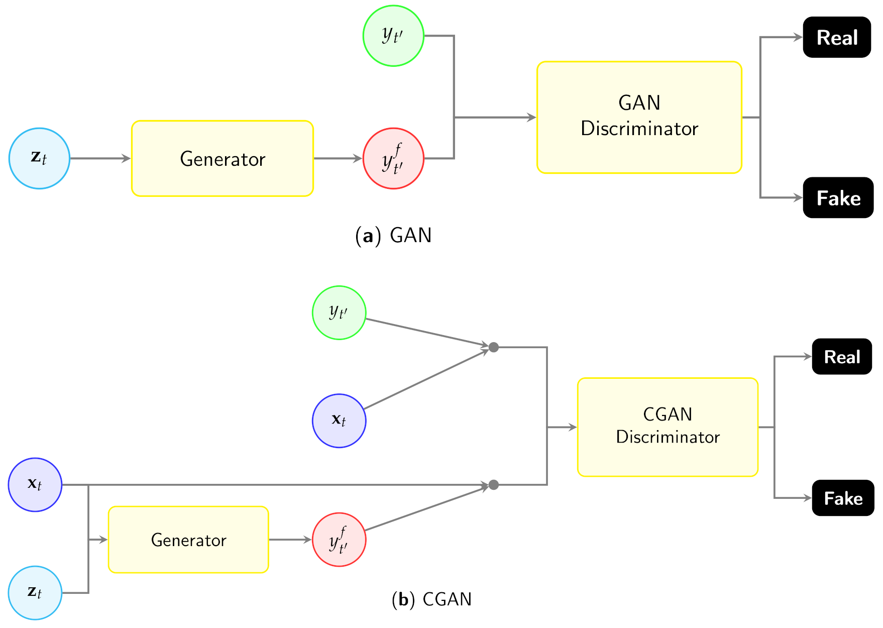
2. The GAN and CGAN Model

The goal of the GAN model is to estimate a generative model using an adversarial process [1]. This is achieved by simultaneously training two models. Firstly, a generative model G, that, in the case of data forecasting, learns past patterns in the data and infers the predictive values. Secondly, a discriminative model D, that determines how likely a sample was to originate from the ‘true’ training data, compared to being sampled from the generator. The generator is, hence, matched against an adversary, the discriminator (whose goal is to detect the difference between a true data sample and one created by the generator). Components of the model are then trained (via an optimization process) to maximize the probability of the discriminator being unable to distinguish true from generated data samples. Typically, including the approach we take here, the generator and the discriminator are both constructed as multi-layer perceptrons, with stochastic gradient methods being employed to obtain optimization.
We start by formulating the definitions which we use in common across the GAN models we test. We consider a time series, y t . Our aim is to estimate the forecast of some y t > t f , conditioned on a set of observations which we denote x t . The inputs to the generator network are x t and z g , where z g is a collection of samples from a normal distribution, p ( z n ) g = N ( 0 , var data ) . During model training, the output from the generator, y t f , as well as the true forecast sample y t , are fed to the discriminator, whose role is to discriminate between them, i.e., to identify y t f as the ‘fake’ sample.
In an unconditioned GAN model, there is no control over the data that is generated. In the CGAN model, in contrast, by conditioning the model on additional information, it is possible to direct the data generation process [2]. Schematics of the GAN and CGAN models are depicted in Figure 1.

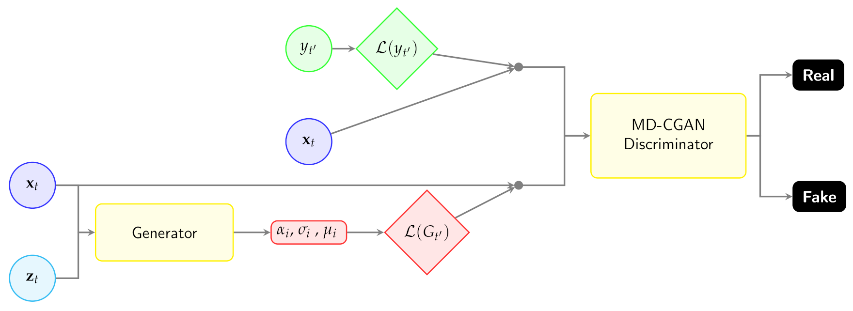
3. The MD-CGAN Model Framework

As with the GAN and CGAN methods, we consider a time series, y t . Our aim now is to infer the posterior distribution over some y t > t , conditioned on the set of observations, x t . In order to form the posterior distribution, we model the full conditional density p ( y t | x t ) as an adversarial network. To achieve this, we use a Mixture Density Network (MDN) model [16] for the generator G. The inputs to the generator network are as per the CGAN approach, x t and z g , where z g is, as before, a collection of samples from a normal distribution, p ( z n ) g = N ( 0 , var data ) . The outputs of G t ( x t , z g ) are now, however, the parameters of the Gaussian mixture posterior over the forecast. This mixture has mixing coefficient, standard deviation, and mean for the i-th component denoted as α i , σ i , and μ i , respectively. As first proposed in Reference [16], we achieve this by using latent variables s = { s α , s σ , s μ } , conditioned on the inputs. The mapping from [ x t , z g ] s { α i , σ i , μ i } is modeled via our network. As the mixings must satisfy i α i = 1 , we map s α to α via the softmax function, where α i = exp ( s α , i ) i exp ( s α , i ) . The elements of σ are strictly positive, so we adopt σ i = exp ( s σ , i ) . Finally, the means can be mapped directly from the latent variables; hence, μ i = s μ , i . Schematically, the MD-CGAN method is depicted in Figure 2.
The above formalism allows us to directly model the predictive likelihood conditioned on an input, and the likelihood of G, conditioned on the observations x t and samples z g as:
L ( G t ( x t , z g ) ) = i = 1 m α i ( x t , z g ) N i ( y t | μ i ( x t , z g ) , σ i ( x t , z g ) ) ,
where m is the number of mixture components.
As in the CGAN model, the discriminator, D, is also conditioned on x t . The input to the discriminator model is, by design, x t 2 π σ a L ( y t ) , where σ a is the standard deviation of the set of observed y t (We note that the GAN approach is not sensitive, within reason, to this value (it is, in effect, a constant in the update equations), and we discuss its setting later in the paper.). For true values of y t , 2 π σ a L ( y t ) is maximized. The generator tries to ‘fool’ the discriminator by generating G t such that the 2 π σ a L ( G t ) is maximized. The loss function for the generator, L G , is as in Equation (2). The discriminator network, on the other hand, attempts to differentiate between true y t values and the pseudo-values created by the generator. The loss function for the discriminator, L D , is as in Equation (3). We note that the lowest value of the discriminator loss is achieved when 2 π σ a L ( y t ) is maximal (unity), and L ( G t ( x t , z g ) ) is minimal (zero).
L G = E z P z ( z ) [ L ( G t ( x t , z g ) ) ] ,
L D = E y P data ( y ) [ x t 2 π σ a L ( y t ) x t 2 ] +     E z P z ( z ) [ x t 2 π σ a L ( G t ( x t , z g ) ) 2 ] .
Our algorithm, thus, follows the steps in Algorithm 1 below.
Algorithm 1 MD-CGAN Algorithm.
1:
for number of training iterations do
2:
    for j steps do do
3:
        Sample N noise samples, { z 1 ,..., z N } from p g ( z )
4:
        Sample N data points, { x 1 ,..., x N } from p data ( x )
5:
        Update the discriminator by descending its stochastic gradient:
θ L n = 1 N [ x ( n ) 2 π σ a L ( y ( n ) ) x ( n ) 2 + x ( n ) 2 π σ a L ( G ( z ( n ) , x ( n ) ) ) 2 ]
6:
    end for
7:
    Sample N noise samples, { z 1 ,..., z N } from p g ( z )
8:
    Update the generator by descending its stochastic gradient:
θ g n = 1 N L ( G ( z ( n ) , x ( n ) ) )
9:
end for

4. Experiments

4.1. Comparison with Other Learning Models

To provide a range of comparisons to methods related to this work, we compare our MD-CGAN model to the following baseline methods: the Mixture Density Network model (MDN), chosen to baseline mixture density outputs against [16]; the CGAN model, chosen as a well-known GAN approach [2]; and a “standard” Multi-Layer Perceptron (MLP) neural network (SNN) as a simple, yet effective, baseline. As a more traditional, parametric, benchmarking model, we use regular (linear-Gaussian) Auto-Regressive (AR) models [17], with parameters obtained by standard least-squares maximum-likelihood estimation. To promote as fair comparison as possible for the nonlinear methods, we use a common neural network architecture across core components in the models, choosing the neural network structure commonly used for GAN models in recent literature [2]. We do not alter this structure throughout our experiments, and we keep to fixed hyperparameter settings (guided by those used in Reference [2]). Figure 3 provides a schematic of the structure used. We note that, whilst the lengths of the input and output vectors are dependent on the model, the structure of all networks remains constant.

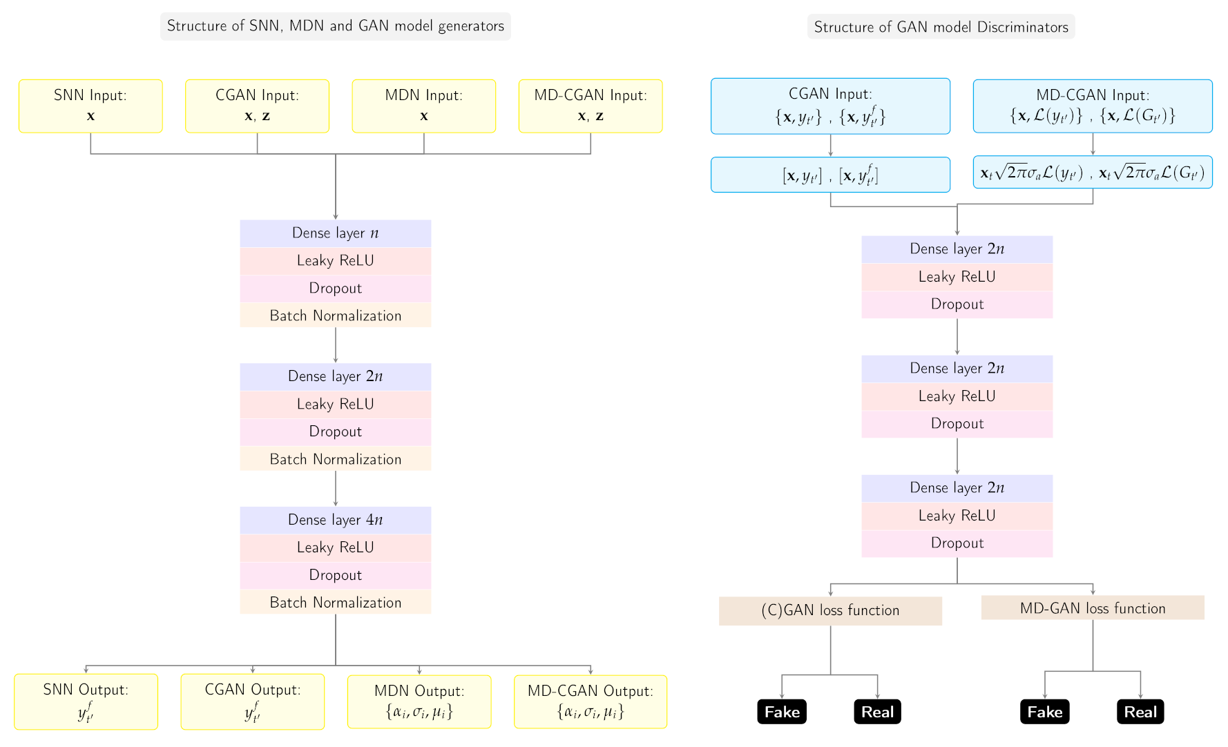
4.2. Details of Implementation

All models were coded in the Python language, and we use the Keras library [18] to build the neural networks.
The neural networks in Figure 3 follow the structure of the CGAN model detailed in Reference [2]. The hyperparameters in the models were set as follows: for the discriminator, both in CGAN and MD-CGAN, the dropout parameter is set to 0.4, and alpha for the leaky ReLU is set to 0.2. For the generator, the dropout rate is set to 0.5, and alpha for the leaky ReLU is, again, 0.2. The parameter governing the number of neurons, n, in the dense layers of the neural network modules is set to 40. The variance parameter, σ a , in the MD-CGAN models is set to 0.2. During training, we follow the steps of Algorithm 1 and set j to 1 for all datasets.
The number of training iterations is, however, specific to model and dataset. With the exception of the GAN models, we monitor the errors, until they reach saturation during training. For the GAN models, in which both the generator and the discriminator have a loss value per iteration, we monitor the average sample error from the training data and continue iteration until the errors reach saturation.
In all models, we optimize parameters using the Adam optimizer [19], with learning rate set to 0.001, exponential decay for the first momentum set to 0.9, exponential decay for the second momentum set to 0.999, and epsilon set to 10 7 .

4.3. Data

We perform experiments on ten datasets with differing provenance, including Mackey-Glass chaotic dataset [20], the Sunspot dataset [21], and eight financial time series. We first look at the one-step forecasting and the issue of (test set) noise resilience, focusing on controlled experiments with the Mackey-Glass and Sunspot datasets (Section 4.4). We then expand our experiments to consider the financial datasets and increased forecast horizon in Section 4.5.
For all datasets we use, the time series is split into training and out-of-sample test sets. The training datasets in all our experiments are comprised of 2000 samples, and all test sets consist of 400 sequential data points post the training set. All performance metrics are obtained from the test set only. To enable a simple comparison across all models and datasets, we keep a fixed lookback window of data as input. All models are, therefore, provided, as input, with the last k data points, set to k = 5 for the purpose of all our experiments. Of course, in practice, the lookback window (or other observation vector) would be optimized for a model and dataset, typically using shrinkage, model-complexity penalties or cross-validation methods [16]. Our goal in this paper is to showcase like-for-like performance when exactly the same observation vector is available across all models. We run both an AR(5) model (corresponding to the common k = 5 observation vector) and, as a martingale baseline, the AR(0) model, in which the forecast is simply the previous observation. All datasets are pre-normalized to the [0,1] interval, again to allow for simpler comparison across data and methods. We further note that both the CGAN and SNN models make point estimate predictions, whilst MD-CGAN and MDN estimate posterior distributions. To enable a simple comparison across models, therefore, we report the mean-square error (MSE) for all methods. The number of mixture components, m, in both MD-CGAN and MDN is set to unity (we vary this in Section 4.6), to further ease comparison across models, some of which produce a probability distribution at output and others point values. The posterior mean of the predictive distribution is taken as the forecast value for both the MDN and MD-CGAN models for the purposes of point-prediction error reporting. Selecting m > 1 for the MD-CGAN and MDN methods would, in principle, be possible, but, as the posterior distribution is non-Gaussian (it is a mixture of Gaussians), the associated error metric is no longer a simple MSE, making like-for-like comparison to other approaches difficult.

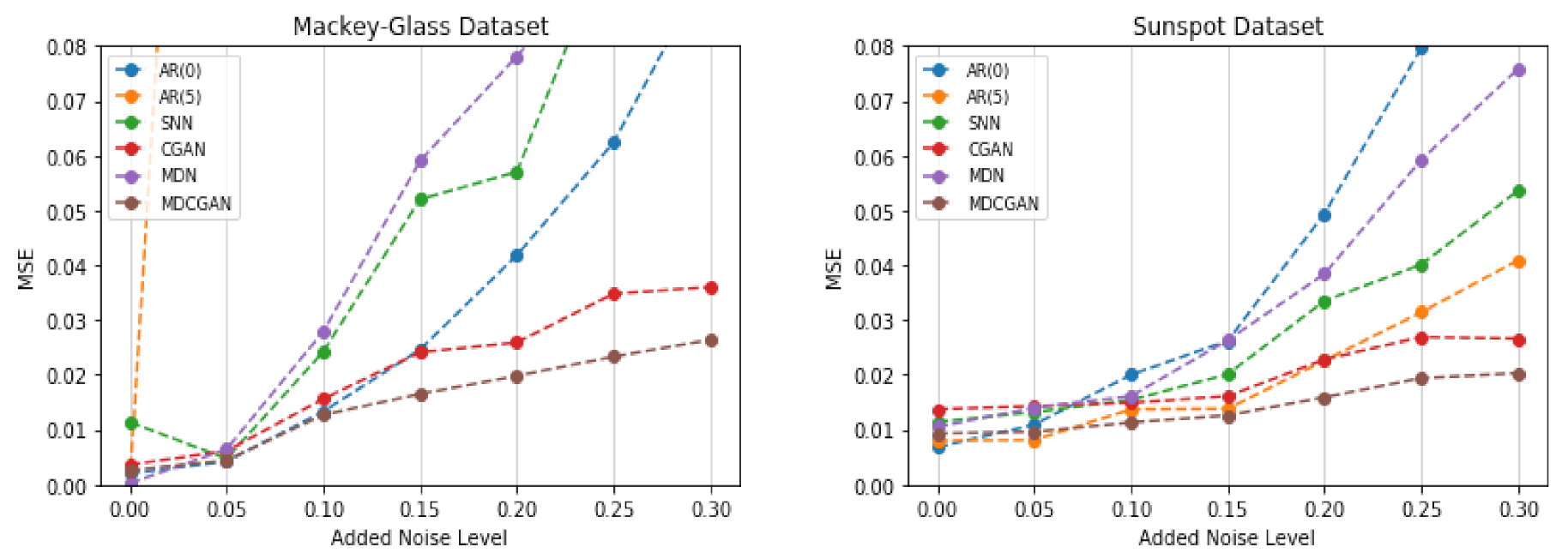
4.4. One-Step Forecasting

Mackey-Glass and Sunspot time series: We start our experiments looking at one-step ahead forecasts on two well known datasets, the Mackey-Glass chaotic time series [20] and the Sunspot dataset [21]. We consider one-step forecast errors in the presence of increasing test set noise. We add 5% to 30% (by amplitude) normally distributed noise to the test data (from a GAN perspective, these input perturbations are, in effect, treated similarly to adversarial attacks). However, a true adversarial attack has an intelligently chosen perturbation to maximize malicious impact. We note that no noise (perturbation) is added to the training dataset. Mean Square Errors (MSE) are presented in Table 1 and Table 2 and Figure 4 for all algorithms considered. For both datasets, we see that MD-CGAN has the best performance for noise levels of 10% and above. Indeed, we see that the GAN models (particularly MD-CGAN) perform consistently well (especially in the Mackey-Glass example) across multiple noise levels, indicating that the approach is particularly resilient to additive observation noise. This is to be expected, as GAN approaches treat the additive noise as adversarial perturbation to the input, against which they are designed to be robust.
In the next section, we investigate model performance at longer forecast horizons, mainly in the finance domain, which is known to contain variable amounts of stochasticity. Financial times series are often dominated by stochastics, and we expect GAN approaches to be well-suited to forecasting in these circumstances.

4.5. Forecasts over Longer-Horizons

One-step forecasts were presented in Section 4.1. Here, we extend analysis over longer horizons. All models make estimates over a horizon of ten weeks for an extended set of financial time series, namely: U.S. initial jobless claims (USIJC, weekly intervals [22]); EURUSD foreign exchange daily rates (EURUSD FX rate [23]), WTI crude oil spot prices (WTI [24]), Henry Hub Natural Gas spot prices (Nat Gas [24]), CBOE Volatility Index (VIX [25]), New York Harbor No. 2 Heating Oil Spot Price (Heating Oil [24]), Invesco DB U.S. Dollar Index Bullish Fund (USD Index [26]), and iShares MSCI Brazil Small-Cap ETF (EM ETF [27]), as well as two other time series: Number of daily births in Quebec (DBQ, [28]) and minimum daily temperatures in the city of Caribou, Maine, USA (MDT [29]). We forecast over a ten-week horizon, representing a 50-step forecast for the daily datasets (FX, WTI, Nat Gas, VIX, Heating Oil, USD Index, EM ETF, DBQ, and MDT), and 10 steps for the weekly USIJC dataset. Our comparisons, as previously, include standard econometric linear models, namely the 5-th order autoregressive, AR(5), model and the martingale, or AR(0) model, in which the forecast is the last observed datum. Taking the martingale model as a baseline, we present in Table 3 the mean-square errors as the ratio to the martingale model error. We note that the MD-CGAN approach delivers ratios below unity and provides the lowest error of almost all models in this scenario.

4.6. Multi-Modal Posterior Predictions

Finally, we compare the performance of MD-CGAN over varying numbers of mixture components. In all the previous experiments, we set m = 1 (hence, the model produced a single predictive Gaussian posterior). Here, we briefly present the results for the finance datasets with m { 1 , 2 , 3 } . We report (negative) log-likelihood measures (as we do not compare against point-value models in this section) and consider one-step forecasts on all the datasets. Table 4 presents the performance across datasets for varying numbers of mixture components in the posterior prediction. Figure 5 shows the predicted distribution for the test datasets for Nat Gas and Vix Index.
We note performance improvement for some datasets for m > 1 . We do not attempt to infer m, though choosing its value based on performance on a set of cross-validation data would be an option, as would enforcing regularization over the mixture model posterior, through more extensive use of Bayesian inference. We leave these extensions for future research.

5. Conclusions

In this paper, we present the MD-CGAN model, which offers extensions to the CGAN [2] methodology, particularly to allow for GAN inference of a (multi-modal) posterior distribution over forecast values. Our approach uses a CGAN-like approach to infer the hyperparameters of a Gaussian Mixture model posterior, and we find that the MD-CGAN approach outperforms other methods on all datasets in which noise is prevalent, including all the financial time series investigated, over long-term forecast horizons. Although the method performs well across all tested datasets, in cases in which strong correlations exist in the time series and little noise is expected at test time, alternative forecasting methods (including neural networks and a range of parametric models) may perform equally well. As a GAN model, our approach retains “adversarial” robustness to data perturbations when forecasting. We find this is most notable when noise is extensively present in data. Our method is, thus, particularly well suited to dealing with financial data. Furthermore, MD-CGAN can effectively estimate a flexible posterior distribution, in contrast to standard GAN models which (almost without exception) produce point value outputs. Exploiting this rich, multi-model, posterior distribution is not reported in detail here but will be featured in follow-up work. In the experiments reported here, “adversarial” perturbations of the observed test data are due to stochastics in the data, rather than carefully planned malicious attacks. Assessing the performance of the model in data with optimized adversarial attacks is an interesting avenue of future research that might be of value in finance, where “spoofing” is often prevalent. In this paper, we do not optimize the lookback window or the structure of the MD-CGAN model for each dataset. Optimization of lookback, and performing neural architecture search, is an interesting avenue for future research, likely to improve performance on a dataset by dataset basis. In summary, the MD-CGAN model combines the advantageous features of both flexible probabilistic forecasting and GAN methods. We see this as a particularly useful approach for dealing with time series in which noise is significant and for providing robust, long-term forecasts beyond simple point estimates.

Author Contributions

Conceptualization, J.Z., S.R.; methodology, J.Z., S.R.; software, J.Z.; validation, J.Z., S.R.; formal analysis, J.Z, S.R.; Investigation, J.Z., S.R.; data curation J.Z.; writing—original draft preparation, J.Z.; writing—review and editing, S.R..; visualization, J.Z., S.R.; supervision, S.R.; project administration, S.R.. All authors have read and agreed to the published version of the manuscript.

Funding

This research received no external funding.

Institutional Review Board Statement

Not applicable.

Informed Consent Statement

Not applicable.

Data Availability Statement

The data presented in this study are openly available with links provided in the References Section.

Acknowledgments

The authors would like to thank the UK Economic and Social Research Council, the Oxford-Man Institute of Quantitative Finance, and the UK Royal Academy of Engineering.

Conflicts of Interest

The authors declare no conflict of interest.

References

  1. Goodfellow, I.; Pouget-Abadie, J.; Mirza, M.; Xu, B.; Warde-Farley, D.; Ozair, S.; Courville, A.; Bengio, Y. Generative adversarial nets. Adv. Neural Inf. Process. Syst. 2014, 27, 2672–2680. [Google Scholar]
  2. Mirza, M.; Osindero, S. Conditional generative adversarial nets. arXiv 2014, arXiv:1411.1784. [Google Scholar]
  3. Wu, H.; Gu, B.; Wang, X.; Pickert, V.; Ji, B. Design and control of a bidirectional wireless charging system using GAN devices. In Proceedings of the 2019 IEEE Applied Power Electronics Conference and Exposition (APEC), Anaheim, CA, USA, 17–21 March 2019; pp. 864–869. [Google Scholar]
  4. Hodge, J.A.; Mishra, K.V.; Zaghloul, A.I. Joint multi-layer GAN-based design of tensorial RF metasurfaces. In Proceedings of the 2019 IEEE 29th International Workshop on Machine Learning for Signal Processing (MLSP), Pittsburgh, PA, USA, 13–16 October 2019; pp. 1–6. [Google Scholar]
  5. Barth, C.B.; Assem, P.; Foulkes, T.; Chung, W.H.; Modeer, T.; Lei, Y.; Pilawa-Podgurski, R.C. Design and control of a GAN-based, 13-level, flying capacitor multilevel inverter. IEEE J. Emerg. Sel. Top. Power Electron. 2019, 8, 2179–2191. [Google Scholar] [CrossRef]
  6. Esteban, C.; Hyland, S.L.; Rätsch, G. Real-valued (Medical) Time Series Generation with Recurrent Conditional GANs. arXiv 2017, arXiv:1706.02633. [Google Scholar]
  7. Wiese, M.; Knobloch, R.; Korn, R.; Kretschmer, P. Quant GANs: Deep Generation of Financial Time Series. Quant. Financ. 2020, 20, 1419–1440. [Google Scholar] [CrossRef] [Green Version]
  8. Zhou, X.; Pan, Z.; Hu, G.; Tang, S.; Zhao, C. Stock market prediction on high-frequency data using generative adversarial nets. Math. Probl. Eng. 2018, 2018, 4907423. [Google Scholar] [CrossRef] [Green Version]
  9. Luo, Y.; Cai, X.; Zhang, Y.; Xu, J.; Xiaojie, Y. Multivariate time series imputation with generative adversarial networks. Adv. Neural Inf. Process. Syst. 2018, 31, 1596–1607. [Google Scholar]
  10. Yu, Y.; Zhou, W.J. Mixture of GANs for Clustering. In Proceedings of the International Joint Conference on Artificial Intelligence, Stockholm, Sweden, 13–19 July 2018; pp. 3047–3053. [Google Scholar]
  11. Gurumurthy, S.; Kiran Sarvadevabhatla, R.; Venkatesh Babu, R. Deligan: Generative adversarial networks for diverse and limited data. In Proceedings of the IEEE Conference on Computer Vision and Pattern Recognition, Honolulu, HI, USA, 21–26 July 2017; pp. 166–174. [Google Scholar]
  12. Ben-Yosef, M.; Weinshall, D. Gaussian mixture generative adversarial networks for diverse datasets, and the unsupervised clustering of images. arXiv 2018, arXiv:1808.10356. [Google Scholar]
  13. Eghbal-zadeh, H.; Zellinger, W.; Widmer, G. Mixture density generative adversarial networks. In Proceedings of the IEEE Conference on Computer Vision and Pattern Recognition, Long Beach, CA, USA, 16–20 June 2019; pp. 5820–5829. [Google Scholar]
  14. Yoon, J.; Jarrett, D.; van der Schaar, M. Time-series Generative Adversarial Networks. In Advances in Neural Information Processing Systems; Curran Associates, Inc.: Vancouver, BC, Canada, 2019; Volume 32. [Google Scholar]
  15. Richardson, E.; Weiss, Y. On GANs and GMMs. In Proceedings of the International Conference on Neural Information Processing Systems, Montreal, QC, Canada, 8–13 December 2018; pp. 5847–5858. [Google Scholar]
  16. Bishop, C.M. Pattern Recognition and Machine Learning; Springer: New York, NY, USA, 2006. [Google Scholar]
  17. Papoulis, A. Probability, Random Variables, and Stochastic Processes; McGraw–Hill: New York, NY, USA, 1984. [Google Scholar]
  18. Chollet, F. Keras. 2015. Available online: https://keras.io (accessed on 30 April 2018).
  19. Kingma, D.P.; Ba, J. Adam: A method for stochastic optimization. arXiv 2014, arXiv:1412.6980. [Google Scholar]
  20. Mackey, M.C.; Glass, L. Oscillation and chaos in physiological control systems. Science 1977, 197, 287–289. [Google Scholar] [CrossRef] [PubMed]
  21. Clette, F. WDC-SILSO. 2015. Available online: http://www.sidc.be/silso/ (accessed on 20 September 2018).
  22. Bureau of Labor Statistics, United States Department of Labor. 2018. Available online: https://www.bls.gov/ (accessed on 20 September 2018).
  23. Investing.com. Euro US Dollar Daily Price. 2018. Available online: https://www.investing.com/currencies/eur-usd-historical-data (accessed on 20 September 2018).
  24. U.S. Energy Information Administration. 2020. Available online: https://www.eia.gov/ (accessed on 15 March 2020).
  25. Microsoft Corp. (MSFT), Yahoo!Finance. CBOE Volatility Index Historical Data. 2020. Available online: https://finance.yahoo.com/quote/%5EVIX/history?p=%5EVIX (accessed on 15 March 2020).
  26. Microsoft Corp. (MSFT), Yahoo!Finance. Invesco DB US Dollar Index Bullish Fund Historical Data. 2020. Available online: https://finance.yahoo.com/quote/UUP/history?p=UUP (accessed on 10 June 2020).
  27. Microsoft Corp. (MSFT), Yahoo!Finance. iShares MSCI Brazil Small-Cap ETF Historical Data. 2020. Available online: https://finance.yahoo.com/quote/EWZS/history?p=EWZS (accessed on 10 June 2020).
  28. Hipel, K.W.; McLeod, A.I. Number of Daily Births in Quebec, 1 January 1977 to 31 December 1990. 1994. Available online: https://datamarket.com/data/set/235j (accessed on 30 September 2018).
  29. National Centres for Environmental Information. Minimum Daily Temperatures in Caribou, ME, USA, 1940–1950. 2021. Available online: https://www.ncdc.noaa.gov/cdo-web/datasets (accessed on 10 July 2021).
Figure 1. Schematic of (a) GAN and (b) CGAN models, showing Generator and Discriminator components and associated variables.
Signals 02 00034 g001
Figure 2. Schematic of the MD-CGAN model. We note that the discriminator in the MD-CGAN model has a different loss function and structure to the GAN and CGAN models.
Signals 02 00034 g002
Figure 3. Common Neural Network structure used across all models.
Signals 02 00034 g003
Figure 4. Comparative MSE plots with increasing test set noise perturbation. We note that the GAN-based methods, particularly MD-CGAN, perform consistently even as noise levels increase.
Signals 02 00034 g004
Figure 5. Estimated distributions for (left) Nat Gas with m = 2 and (right) VIX index with m = 1 over out-of-sample test datasets. True samples are shown as white dots. Red indicates high data likelihood, and blue data low likelihood, under the MD-CGAN model.
Signals 02 00034 g005
Table 1. Mackey-Glass data: MSE variation with added noise level, with standard deviations in parentheses.
0% Noise5% Noise10% Noise15% Noise20% Noise25% Noise30% Noise
AR(0)0.00200.00420.01330.02460.04180.06240.0951
( 0.0000 ) ( 0.0000 ) ( 0.0000 ) ( 0.0000 ) ( 0.0000 ) ( 0.0000 ) ( 0.0000 )
AR(5)4.1 × 10 6 0.27941.15582.65814.48687.315210.1527
( 0.0000 ) ( 0.0000 ) ( 0.0000 ) ( 0.0000 ) ( 0.0000 ) ( 0.0000 ) ( 0.0000 )
SNN0.00140.00470.02420.05190.05700.10130.1640
( 0.0000 ) ( 0.0001 ) ( 0.0015 ) ( 0.0014 ) ( 0.0021 ) ( 0.0023 ) ( 0.0099 )
CGAN0.00360.00610.01550.02400.02590.03470.0360
( 0.0002 ) ( 0.0004 ) ( 0.0009 ) ( 0.0009 ) ( 0.0013 ) ( 0.0012 ) ( 0.0012 )
MDN0.00020.00640.02780.05890.07800.09800.1402
( 0.0000 ) ( 0.0001 ) ( 0.0007 ) ( 0.0011 ) ( 0.0012 ) ( 0.0012 ) ( 0.0011 )
MD-CGAN0.00260.00440.01260.01650.01970.02330.0264
( 0.0001 ) ( 0.0002 ) ( 0.0002 ) ( 0.0004 ) ( 0.0007 ) ( 0.0008 ) ( 0.0006 )
Table 2. Sunspot data: MSE variation with added noise level, with standard deviations in parentheses.
0% Noise5% Noise10% Noise15% Noise20% Noise25% Noise30% Noise
AR(0)0.00800.01090.02000.02620.04940.07950.0974
( 0.0000 ) ( 0.0000 ) ( 0.0000 ) ( 0.0000 ) ( 0.0000 ) ( 0.0000 ) ( 0.0000 )
AR(5)0.00680.00810.01370.01380.02260.03140.0409
( 0.0000 ) ( 0.0000 ) ( 0.0000 ) ( 0.0000 ) ( 0.0000 ) ( 0.0000 ) ( 0.0000 )
SNN0.01140.01320.01540.02010.03350.04010.0536
( 0.0004 ) ( 0.0006 ) ( 0.0008 ) ( 0.0009 ) ( 0.0014 ) ( 0.0022 ) ( 0.0025 )
CGAN0.01370.01430.01490.01610.02280.02690.0266
( 0.0002 ) ( 0.0008 ) ( 0.0012 ) ( 0.0010 ) ( 0.0022 ) ( 0.0021 ) ( 0.0023 )
MDN0.01050.01400.01610.02630.03840.05920.0758
( 0.0000 ) ( 0.0008 ) ( 0.0013 ) ( 0.0013 ) ( 0.0018 ) ( 0.0023 ) ( 0.0017 )
MD-CGAN0.00930.00960.01130.01260.01590.01940.0203
( 0.0001 ) ( 0.0002 ) ( 0.0002 ) ( 0.0002 ) ( 0.0003 ) ( 0.0006 ) ( 0.0007 )
Table 3. Ratio of model MSE to martingale, AR(0), baseline model over 10-week forecast horizon.
USIJCEURUSD FX RateWTINat GasVIX IndexHeating OilUSD IndexEM ETFDBQMDT
AR(5)0.781.910.851.010.710.821.240.890.560.65
SNN0.791.250.890.940.710.931.340.820.410.64
CGAN0.770.851.531.070.910.541.370.690.660.69
MDN0.843.481.481.130.770.890.680.810.450.62
MD-CGAN0.730.760.800.820.660.590.540.650.380.61
Table 4. Negative log-likelihood variation with m, with standard deviations in brackets.
USIJCEURUSD FX RateWTINat GasVIX IndexHeating OilUSD IndexEM ETFDBQMDT
m = 1 −1.01−1.79−1.75−1.28−1.50−1.63−0.65−1.26−0.62−0.82
( 0.02 ) ( 0.08 ) ( 0.09 ) ( 0.04 ) ( 0.05 ) ( 0.06 ) ( 0.05 ) ( 0.05 ) ( 0.01 ) ( 0.02 )
m = 2 −1.05−0.98−1.24−1.33−1.39−1.37−0.83−1.10−0.69−0.85
( 0.04 ) ( 0.05 ) ( 0.02 ) ( 0.02 ) ( 0.04 ) ( 0.03 ) ( 0.05 ) ( 0.03 ) ( 0.02 ) ( 0.03 )
m = 3 −1.09−0.67−1.33−1.25−1.48−1.35−0.86−1.09−0.67−0.91
( 0.02 ) ( 0.04 ) ( 0.06 ) ( 0.02 ) ( 0.03 ) ( 0.02 ) ( 0.07 ) ( 0.05 ) ( 0.02 ) ( 0.03 )
Publisher’s Note: MDPI stays neutral with regard to jurisdictional claims in published maps and institutional affiliations.

