
Recovering Texture with a Denoising-Process-Aware LMMSE Filter


Chiba Institute of Technology, Narashino-shi 275-0016, Japan
*
Author to whom correspondence should be addressed.
Signals 2021, 2(2), 286-303; https://doi.org/10.3390/signals2020019
Submission received: 26 January 2021
/
Revised: 5 March 2021
/
Accepted: 10 May 2021
/
Published: 11 May 2021
Abstract
:Image denoising methods generally remove not only noise but also fine-scale textures and thus degrade the subjective image quality. In this paper, we propose a method of recovering the texture component that is lost under a state-of-the-art denoising method called weighted nuclear norm minimization (WNNM). We recover the image texture with a linear minimum mean squared error estimator (LMMSE filter), which requires statistical information about the texture and noise. This requirement is the key problem preventing the application of the LMMSE filter for texture recovery because such information is not easily obtained. We propose a new method of estimating the necessary statistical information using Stein’s lemma and several assumptions and show that our estimated information is more accurate than the simple estimation in terms of the Fréchet distance. Experimental results show that our proposed method can improve the objective quality of denoised images. Moreover, we show that our proposed method can also improve the subjective quality when an additional parameter is chosen for the texture to be added.
1. Introduction
Image denoising methods that can estimate a noiseless, clean natural image (original image) from a noisy observation are actively being studied [1,2,3,4,5,6,7,8,9,10,11,12,13,14,15,16,17,18,19,20,21]. Many previous works have assumed that the noise in such a noisy observation is an additive white Gaussian noise (AWGN). One popular approach for image denoising is to use nonlocal self-similarity (NLSS), in which it is assumed that a local segment of an image (a patch) is similar to other local patches [10,11,12,13,14,15,16,17,18,19,20,21].
Weighted nuclear norm minimization for image denoising (WNNM) [16] is an optimization-based method based on an NLSS-based objective function. WNNM assumes that a matrix whose columns consist of similar patches extracted from a clean image is low rank and achieves state-of-the-art denoising performance among non-learning-based methods.
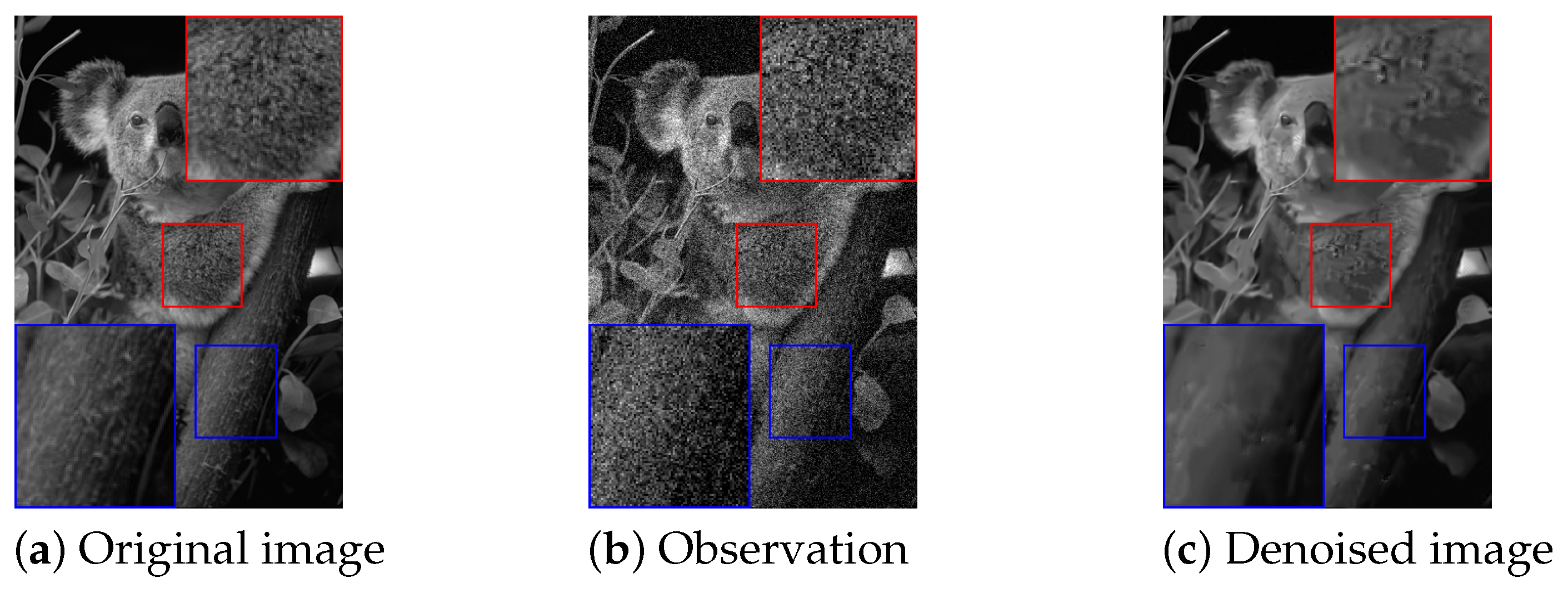
Image denoising methods such as WNNM can estimate the original image well in terms of the mean squared error (MSE) or the peak-signal-to-noise ratio (PSNR). However, as shown in Figure 1, texture is often lost in the estimated image. Because the texture carries important information about the aesthetic properties of the materials depicted in certain parts of an image (such as the feel of sand, fur, or tree bark), the texture losses severely degrade the subjective image quality.
On the other hand, it is difficult to obtain a good description of texture (we refer to such a description as a texture model) and to estimate its parameters because of its stochastic nature, and the performance of texture-aware image denoising methods [8,19,20,21] depends on these models and parameters. Thus, we can classify texture-aware image denoising methods based on the texture models they utilize.
The gradient histogram preservation (GHP) method [19] is a prominent texture model for texture-aware image denoising. GHP describes texture features in the form of a histogram of the spatial gradients of the pixel values (gradient histogram). GHP is based on an image denoising method called nonlocally centralized sparse representation [15], and it can recover texture by imposing the condition that the gradient histogram of the output image must be close to that of the original image. The parameters of GHP can be estimated from the observed image by solving an inverse problem.
However, GHP does not utilize the relationships between distant pixels. Nevertheless, these relationships can carry important texture information because textures are often repeated over long distances.
Zhao et al. addressed this problem by proposing a texture-preserving denoising method [20] that groups similar texture patches through adaptive clustering and then applies principal component analysis (PCA) and a suboptimal Wiener filter to each group. The Wiener filter is a special case of a linear minimum mean squared error estimator (LMMSE filter), and it requires an estimation of the covariance matrices of the original signals. In this texture model, the relationships between distant pixels can be expressed by the covariance matrices. The covariance matrices that are used in the suboptimal Wiener filter are calculated from sample observation patches, which are chosen using a nonfixed search window.
As another method of managing the distant relationships characterizing texture, a denoising method using the total generalized variation (TGV) and low-rank matrix approximation via nuclear norm minimization has been proposed [21]. In this method, the TGV is used to avoid the oversmoothing that is typically caused by low-rank matrix approximation methods [10,16]. The TGV and nuclear norm minimization are applied to capture the relationships between nearby pixels and distant pixels, respectively. Liu et al. claim that the latter are related to textures with regular patterns. The parameter of their texture model is the weight parameter of the TGV term. An iterative algorithm is required to estimate this parameter.
There is a trade-off between the complexity (or capacity) of a texture model and the simplicity of parameter estimation. For example, GHP [19] is a simple texture model with parameters that are easily estimated. However, this model cannot express textures in detail. By contrast, the covariance in the PCA domain [20] and the combination of the TGV and the nuclear norm [21] are complex texture models that can represent detailed textures well; however, their parameter estimation is relatively difficult.
To resolve this problem, we employ a slightly different definition of texture in this paper. We define texture as the difference between the original image and the corresponding denoised image (as obtained from an existing denoiser). We use the covariances within the texture component and between the texture and noise (covariance matrices) as our texture model, thereby capturing information about the relationships between distant pixels. Throughout this paper, we represent the covariance information in matrix form. Thus, we refer to this information as covariance matrices. It would appear to be difficult to estimate these matrices from a noisy observation. However, because we define the texture as the difference between the original and denoised images, we can utilize the information obtained in the denoising process to estimate the texture covariance matrices more easily.
We propose to use Stein’s lemma [22] and several empirical assumptions to estimate the covariance matrices. Then, we apply an LMMSE filter based on the covariance matrices to estimate the lost texture information. In general, the Wiener filter assumes that the target and the noise have zero covariance. However, in our case, there is nonzero covariance between the texture, which is the difference between the original and denoised images, and the noise because the denoised image depends on the noise. Thus, we propose to use the LMMSE filter for the case in which there is covariance between the signal and noise.
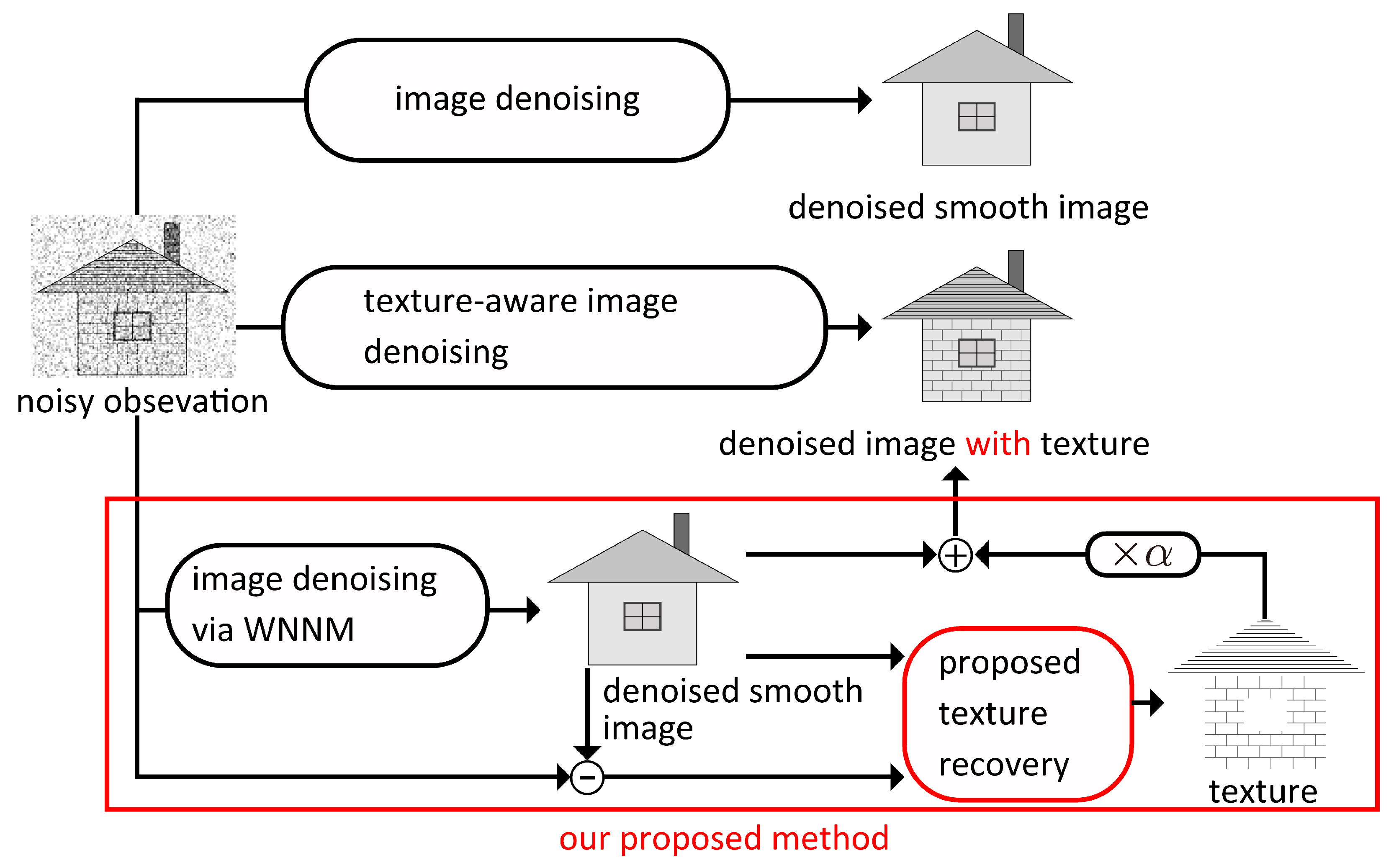
Moreover, our approach yields a separate texture image, which allows us to emphasize the texture with any desired magnitude. Such texture magnification can improve the subjective quality of an image. Figure 2 presents our motivation.
Our contributions are summarized as follows:
- We propose a new definition of texture for texture-aware denoising and a method of recovering texture information by applying an LMMSE filter.
- We introduce several nontrivial assumptions to estimate the covariance matrices regarding the texture and noise that are used in the LMMSE filter based on Stein’s lemma.
- We show an effectiveness of our method in terms of the PSNR and subjective quality (with texture magnification) through experiments. We also show similarities between our estimated covariance matrices and the corresponding true covariance matrices in terms of the Fréchet distance [23].
Recently, several image denoising methods based on neural networks have been proposed [9,18]. These methods achieve excellent denoising performance. However, understanding the process underlying such black-box methods is difficult. To the best of our knowledge, WNNM is still the state-of-the-art among denoising algorithms that are not based on machine learning approaches (i.e., white-box methods), and our proposed method represents the first successful attempt to significantly improve the performance of WNNM. Additionally, our method can explicitly extract the texture component from the noisy image, enabling us to maximize the perceptual quality of the denoised images by arbitrarily magnifying the obtained texture. In the pursuit of the inherent model of natural images, it is worthwhile to improve the denoising performance of white-box algorithms, as accomplished with the proposed method.
This paper is organized as follows. Section 2 introduces WNNM as the background to this study. Section 3 introduces our newly proposed method of texture recovery and analyzes the texture and noise covariance matrices using Stein’s lemma. We propose a linear approximation of WNNM to enable the application of Stein’s lemma. Section 4 compares our method with other state-of-the-art denoising methods. Section 5 concludes the paper. Appendix A proves that our LMMSE filter can successfully estimate the texture component of the original image. Appendix B shows experimental results to confirm our several assumptions.
Please note that this work on texture recovery has been previously presented in conference proceedings [24]. In this paper, we show the proof of the LMMSE filter and experimental results to confirm some assumptions. We also analyze the estimation accuracy of our texture covariance matrix used for texture recovery and the effectiveness of emphasizing the texture statistically. In conference proceedings, we only provided limited experimental results (24 images of Kodak Photo CD PCD 0992). On the other hand, in this paper, we show new experimental results obtained on two image datasets (contains 110 images in total) to confirm our method’s effectiveness.
2. Preliminaries and Notation
In this paper, denotes the set of real numbers, small bold letters denote vectors, and large bold letters denote matrices. We denote the estimates of and by and , respectively.
In this section, we describe WNNM [16] (a state-of-the-art denoising method based on NLSS) because our method estimates the texture information lost via the denoising process in WNNM.
In image denoising, a noisy observation is modeled as
where is the noisy observation with m pixels, is the original image that is the target of estimation, and is AWGN, of which the standard deviation is .
In WNNM, the observed image is first divided into I overlapping focused patches ( pixels). The I depends on the image size and the noise level. Our experiment follows the default parameter of author’s implementation of WNNM. For example, in the case of , the patch size is pixels, and the focused patches are selected by 1 pixel skip (stride 2). Therefore, when the image size is pixels, the total number of focused patches I is 32,004 (note that similar patches are selected from pixels patches extracted from the neighborhood ( pixels) of the focused patch. The overlapping focused patches are then vectorized. We denote the i-th focused patch of by (). Then, a search is performed for the patches that are the most similar to each segmented patch , and for each , a patch matrix is created that includes as its leftmost column, while the remaining columns of are the patches that are similar to . For the i-th patches of the other components and , we use similar notation, i.e., and . We denote their corresponding patch matrices by and . Note that the indices of the similar patches in and are the same as those in .
For simplicity, we subtract the columnwise average of the matrix from each row of and denote the result by . The same columnwise average subtraction method is used in the implementation provided by Gu et al.; however, this is not explicitly described in [16]. Because we assume that is AWGN, each columnwise average of the noiseless matrix is sufficiently similar to that of . Thus, the objective of WNNM is to estimate which is obtained by subtracting the columnwise average of from .
The core of the denoising process of WNNM is the following equation based on the singular value decomposition (SVD) of the observed patch matrix :
where is the denoised patch matrix, is the SVD and is a threshold function. Each component of the diagonal matrix is expressed as
where
C is an arbitrary parameter, and is a small number. This process corresponds to a closed-form solution of the iterative reweighting method applied to the singular value matrix of [16].
The singular value thresholding described above is applied to each focused patch and similar patches, and estimates of the original patches are obtained by adding the columnwise average to . Then, the estimated original patches are combined to obtain a reconstructed image (overlapping patches are subjected to pixelwise averaging). In WNNM, this process is iterated to estimate the original image. In each iteration, the denoising target is updated by calculating a weighted sum of the most recently estimated image and the original noisy observation (where k is the index of the iteration) with a weight parameter , as follows: . This process is called iterative regularization, and the parameter is fixed to in [16]. The WNNM algorithm is given in Algorithm 1. For additional details on WNNM, please consult [16].
| Algorithm 1 Image denoising via WNNM. |
| Input: Noisy observation |
| Initialize and |
| for do |
| Iterative regularization: |
| for do |
| Find the similar patch matrix |
| Estimate the corresponding original patch matrix by applying Equation (2); the result is |
| end for |
| Use the to reconstruct the estimated image |
| end for |
| Output: Obtain the denoised image as |
3. Recovering Texture via Statistical Analysis
In this section, we introduce our denoising method that recovers the texture lost by denoising a noisy observation. In this paper, we define a structure (or cartoon) component , where is a map corresponding to the denoising process of WNNM. Then, in contrast to previous work [8,19,20,21], we define a texture component as the difference between the original image and the structure (i.e., ). Thus, we obtain our extended observation model, i.e.,
Please note that the above equation is equivalent to Equation (1) since . Our goal is to estimate the texture component that has been lost via WNNM.
First, we denoise the observation with WNNM. Following WNNM, we estimate each texture patch matrix from the corresponding structure patch matrix , which is obtained in the final iteration of the WNNM procedure, and the corresponding observation patch matrix . Because we use an LMMSE filter to estimate , we need the statistical information on the relationship between the texture and noise; however, this information cannot be calculated directly because and are not observable. Instead, we estimate this information using Stein’s lemma and several assumptions, which are described below, and then reconstruct the estimated texture patch matrices to obtain the estimated texture component . Finally, we obtain an estimate of the original image, , by adding the estimated texture component to the denoised image .
3.1. LMMSE Filter for Texture Recovery
We use an LMMSE filter to estimate each texture patch . The objective function of the LMMSE filter, is formulated as
where denotes the expected value and is the ℓ − 2 norm. Because this formula is quadratic, we can easily find the minimizer as follows:
where we adopt the following covariance matrix notation: (where and are some random vectors). The proof is given in Appendix A.
Unfortunately, the covariance matrices and cannot be directly obtained because and are not observable. We solve this problem by using Stein’s lemma and introducing several assumptions.
3.2. Estimation of the Covariance Matrices
As mentioned above, we need to estimate and . Since we define as , and the value of is changed with respect to the value of , we can assume that is the output of a function that takes as an input. also follows a normal distribution. Thus, we can estimate using Stein’s lemma as follows:
The above equation shows that our desired covariance matrices can be obtained from the effects of the on the . The texture patch is equal to according to Equation (5); moreover, we assume that the effect of on is zero. Therefore, we can estimate the covariance matrix as
We need to analyze the variations in the WNNM output as the noise varies. As mentioned above, the WNNM process is complex. Thus, we need to approximate the WNNM process with a linear filter to simplify the analysis.
Surprisingly, the linear approximation of the WNNM process also provides us with an empirical method of estimating , which is more difficult to estimate than . In the next subsection, we describe how to approximate WNNM with a linear filter and how to estimate .
3.3. Linear Approximation of the WNNM Procedure
To simplify the analysis and determine the covariance matrix by using Stein’s lemma, we assume that we can precisely approximate the whole process of WNNM as a linear filter:
The SVDs of and are formulated as
If we ignore the fact that the patch matrices are updated in WNNM via a similar patch search, reconstruction and iterative regularization in each iteration, then the SVDs of and will have common right and left singular matrices. We assume that and are equal to and , respectively. Thus, we can obtain the approximate WNNM filter as follows:
The partial derivative of the columnwise average of with respect to is considered to be very small because is Gaussian and because the average of is zero. Note that is obtained by subtracting the columnwise average of from .
If this approximation of WNNM is sufficiently accurate, then . From Equation (9), we can estimate as
Additionally, we use the approximate WNNM filter to estimate . We assume that can be estimated as
This assumption is founded on preliminary experiments. The details of these preliminary experiments are presented in Appendix B.3.
3.4. Recovering the Texture of a Denoised Image
Based on the above discussion, we can calculate the LMMSE filter and estimate . However, is not invertible in practice because the number of patches M is smaller than L. Although an equivalent estimate of appears to be (where is the identity matrix), this choice does not provide good recovery performance. Instead, substituting into the sample covariance matrix was found to yield the best results in our preliminary experiments. Thus, we calculate the LMMSE filter as
Then, we can obtain the desired estimated texture image that is obtained by combining each in the same manner used to reconstruct an image from the patches obtained in WNNM. Finally, we can obtain the final estimated image with enhanced texture as
We use the LMMSE filter to obtain ; however, minimizing the MSE often causes to lose clarity. We can obtain a clearer texture-enhanced image as follows:
where is an arbitrary parameter used to control the magnitude of the texture that is added. Note that means the proposed method applies the LMMSE filter and we can expect to obtain the denoised images with best PSNR if all of our assumptions hold. The entire proposed process is presented in Algorithm 2.
| Algorithm 2 Texture recovery using the proposed method. |
| Input: Noisy observation |
| Initialize and |
| for do |
| Iterative regularization: |
| for do |
| Find the similar patch matrix |
| Estimate the corresponding original patch matrix via Equation (2); the result is denoted by |
| if k=K then |
| Estimate and using Stein’s lemma via Equation (13) and (14) |
| Calculate via Equation (9) |
| Estimate via Equation (16) to obtain |
| end if |
| end for |
| Use the to reconstruct the estimated image |
| end for |
| Use the to reconstruct the estimated texture component |
| Output: Obtain the final estimated image as |
4. Experimental Results
In this section, we discuss our experimental results. First, we present performance of our denoising method and compare it to other non-learning-based state-of-the-art denoising methods, namely, block matching and 3D filtering (BM3D) [11], GHP [19], and WNNM [16]. For comparison with learning-based denoising methods, we compare the denoising performance of the proposed method with that of a denoising convolutional neural network (DnCNN) [9]. We also confirm the effects of the parameter . Moreover, we present a histogram of the Fréchet distance to confirm the assumption of Equation (14).
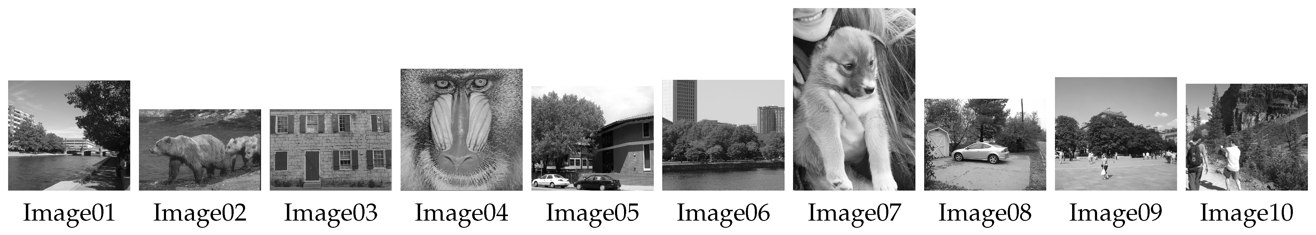
We used two image datasets for validation. One dataset consists of ten grayscale natural images from [21], as shown in Figure 3 (dataset I). The other dataset contains 100 grayscale natural images from the Berkeley segmentation dataset [25] (BSD100). In all experiments, we used MATLAB R2018b for the implementation, and all noisy observations were simulated by adding noise generated by a pseudorandom number generator to the original images.
4.1. Image Denoising
The PSNR and structural self-similarity (SSIM) [26] results for the denoised images from dataset I with different noise levels are given in Table 1, Table 2 and Table 3. Note that higher PSNR and SSIM values mean that the reference image is more similar to the original image. We highlight the highest PSNR and SSIM in each row in bold. We set the texture scaling parameter to because we wish to measure how much improvement is achieved in terms of the PSNR. We recover the texture using the LMMSE filter; thus, the MSE is likely to be low, meaning that the PSNR should be high. These tables show that our denoising method outperforms the other state-of-the-art methods in terms of both the PSNR and SSIM. The largest difference in the PSNR between WNNM and our method is 0.15 dB. Additionally, the averages of the denoising results on BSD100 at each noise level are shown in Table 4. This table shows that the performance improvement achieved with our method is independent of the dataset. For each image in BSD100, we performed one-tailed paired t-tests on the difference of each PSNR and SSIM between the proposed method and WNNM. In this test, the null hypothesis is that the PSNR/SSIM values obtained by proposed method are not greater than the corresponding values obtained by WNNM. The p-values are also shown in Table 4. From the results, since the p-values are small enough, we confirmed statistically significant differences between our proposed method and WNNM.
Moreover, we show the averages of computational time of WNNM and the proposed method in Table 5. The computational times were measured on 10 distinct observed images (the noise value of each observation is different) for each test image from BSD100. The additional computational time of our texture recovery is 7–13% of the computational time of WNNM. The PSNR/SSIM gain obtained by our texture recovery method is considered to be sufficient for the users to accept this additional cost.
We also compare the denoising performance of the proposed method with that of the DnCNN [9] on dataset I. The noise level was set to 15 and the texture scaling parameter was set to 1. We used the PyTorch implementation of DnCNN and the pretrained model parameters for noise level , which is published by the authors of [9]. The experimental results are shown in Table 6. The improvement of DnCNN over WNNM is 0.30 dB in the average of PSNR while that of the proposed method is 0.10 dB. Note that the proposed method requires no training process and is fully explainable while the denoising mechanism of DnCNN is black box.
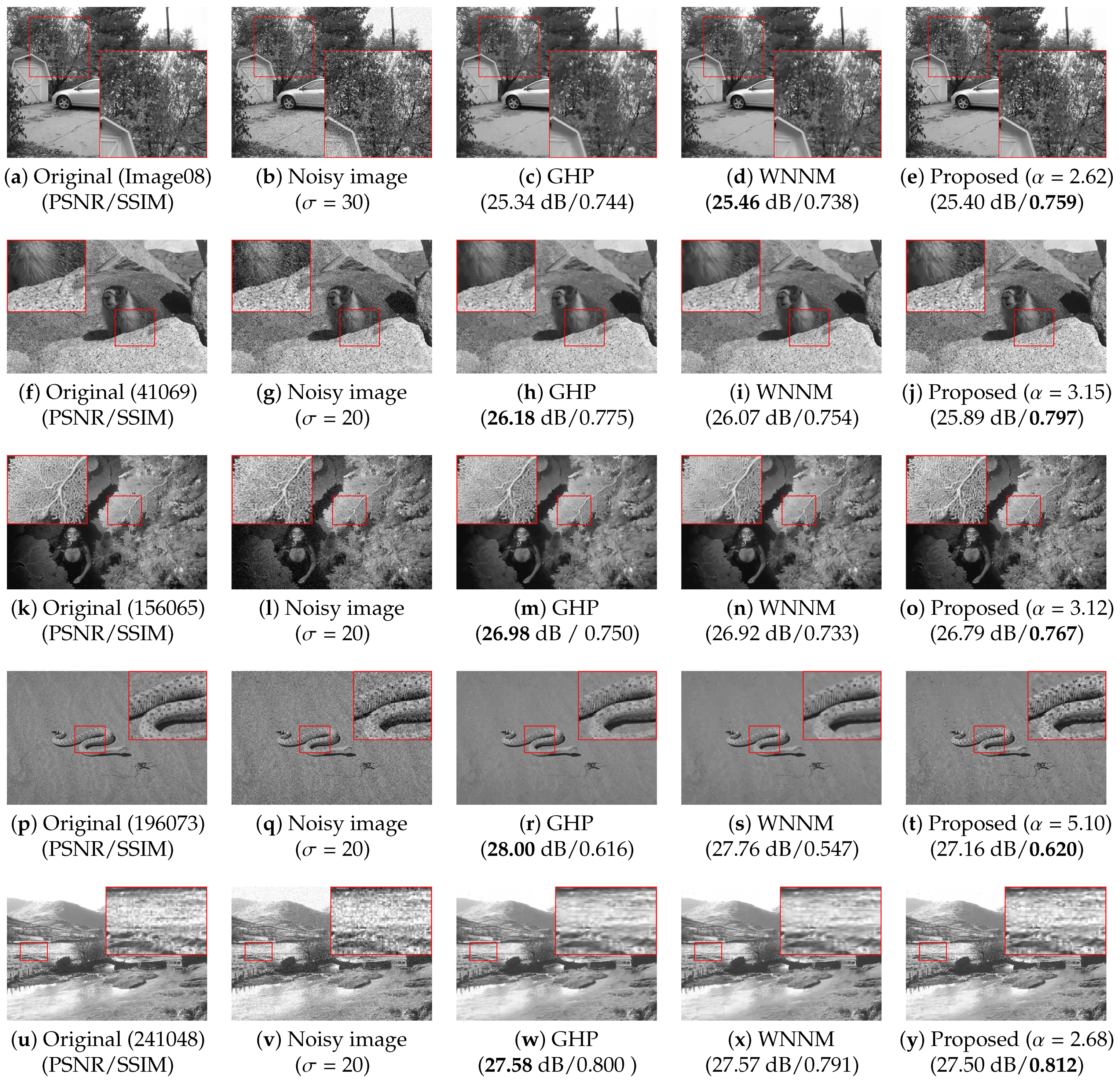
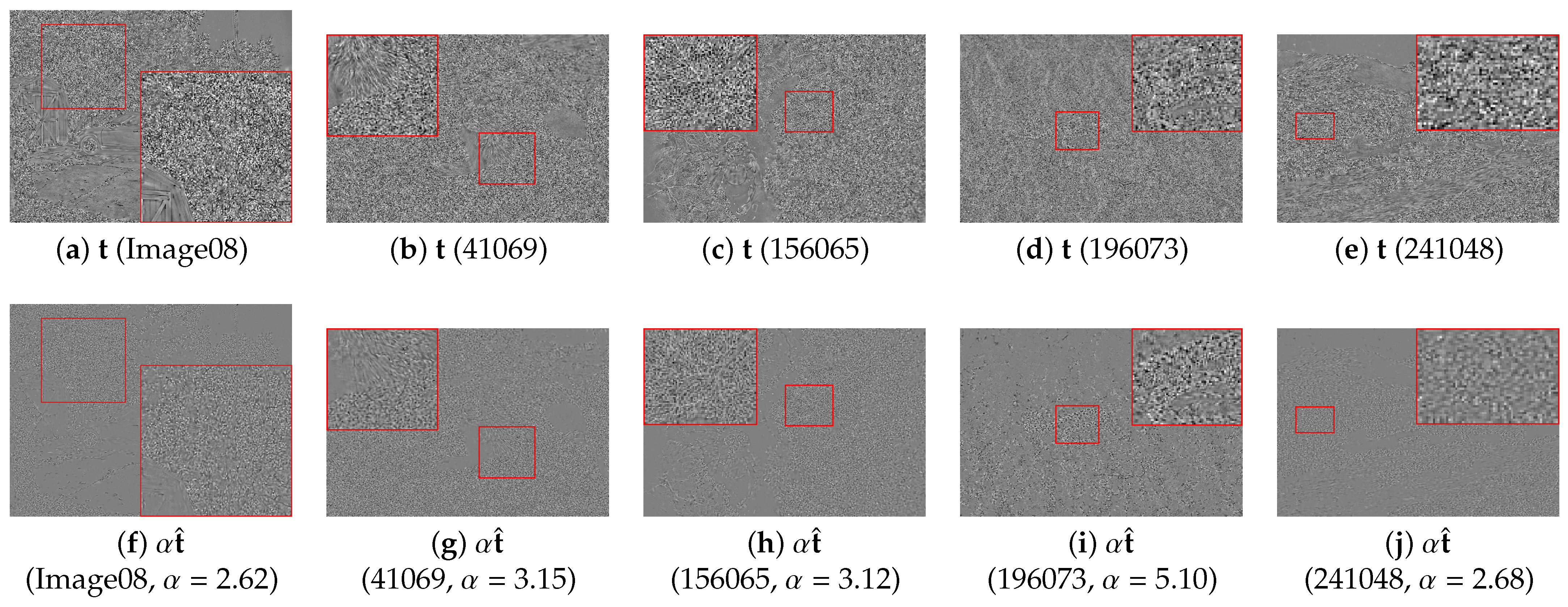
Next, to observe the effect of the parameter , we searched for the value of this parameter that would maximize the SSIM of the output image, denoted by . We obtained via a line search in the range from 0 to 8 in increments of . For several examples, the original image, the noisy observation, the output image obtained via GHP, the output image obtained via WNNM, and an output image obtained with our method are shown in Figure 4. From this figure, we can observe that the subjective quality and SSIM can be drastically improved by properly choosing the parameter . For example, as shown in Figure 4p–t for the image named 196073, the SSIM value obtained with our method is 0.073 higher than that achieved via WNNM. Moreover, we show and of each image of Figure 4 in Figure 5. Please note that the pixel value of each image is multiplied by a factor of 3. This figure shows that is similar to in each textured region such as surface of a stone, a coral, the skin of a snake, and the surface of the sea.
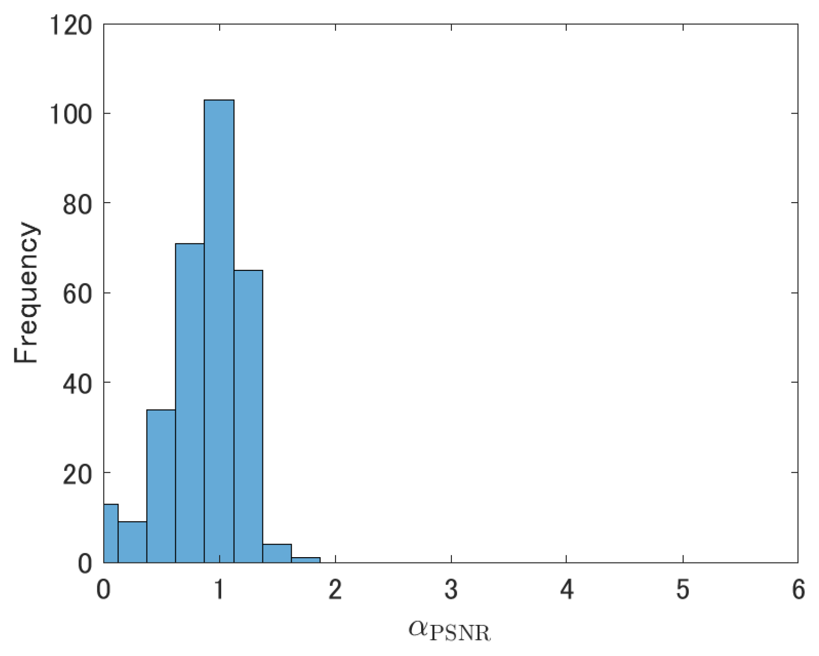
A histogram of the values obtained on BSD100 is shown in Figure 6. We note that this histogram shows the frequency under three noise levels ( = 10, 20, 30). This figure indicates that there is no single optimal value of that is common to all images. Nevertheless, the figure also shows that choosing will almost always increase the expected value of the SSIM. Moreover, as with , we searched for the value of that would maximize the PSNR of the output image, and denoted it by . We obtained for each image via a line search in the range from 0 to 8 in increments of . Figure 7 shows a histogram of the values of . We confirmed that produces the denoised images with the best PSNR in most cases.
4.2. Accuracy of Texture Covariance Matrix Estimation
In this section, we compare the accuracy of two texture covariance matrices. One is our estimated texture covariance matrix, and the other is a simply sampled estimate that is calculated as
where is a function that replaces any negative eigenvalues of the input matrix with zero; this is equivalent to metric projection to a positive-semidefinite matrix.
We calculate the Fréchet distance to evaluate the accuracy of the texture covariance matrix. Dowson and Landau introduced the calculation of the Fréchet distance between multivariate normal (MVN) distributions [23]. The Fréchet distance is also used to measure the similarity between generated and real images [27]. We assume that the texture component follows an MVN distribution. Consider a random MVN-distributed variable whose mean vector is and whose covariance matrix is (); its probability density is denoted by
Additionally, the Fréchet distance between the MVN distributions and is calculated as
We assume that the mean vector of the texture is . Thus, we can calculate the Fréchet distance between the estimated texture covariance matrix and the true texture covariance matrix from the ground truth as follows:
We can similarly calculate the Fréchet distance between the simply sampled estimate and by replacing with in Equation (22).
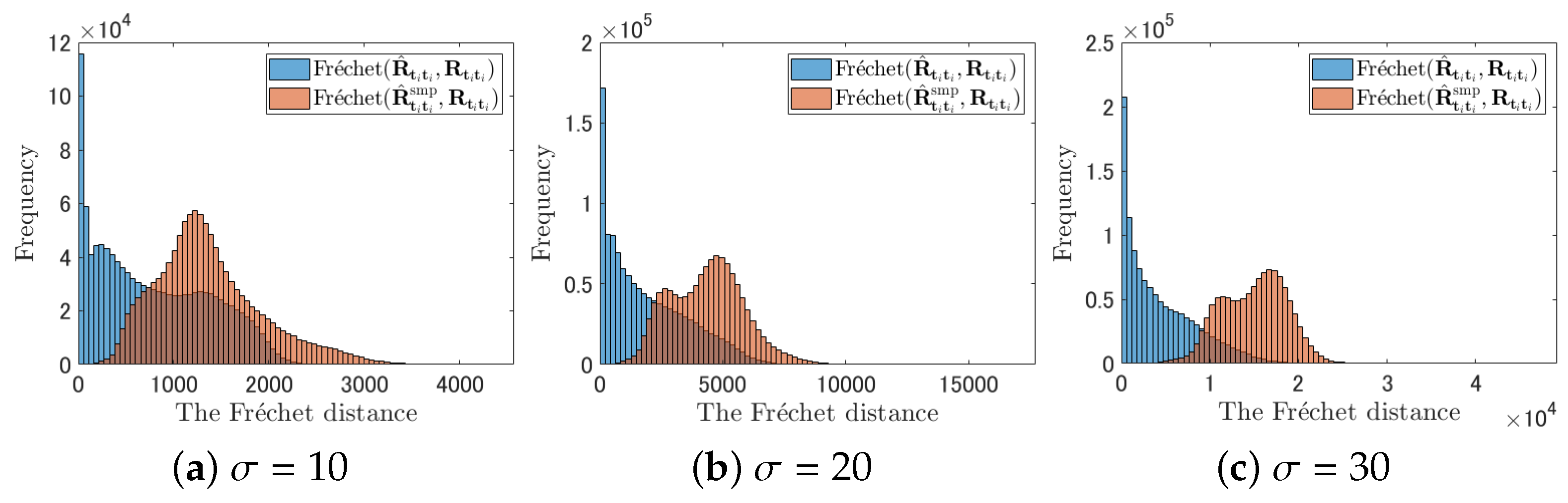
Figure 8 shows histograms of these Fréchet distances. Note that we calculated the Fréchet distance for each patch matrix from dataset I. However, we ignored the very few outliers caused by numerical errors. This figure shows that is more similar to than is at each noise level.
5. Conclusions
In this paper, we have proposed a method of recovering texture information that has been oversmoothed by the denoising process in WNNM. For texture recovery, we apply an LMMSE filter to a noisy image. Because our filter requires covariance matrices between the texture and noise, we have also proposed a method of estimating this information based on Stein’s lemma and several key assumptions.
Experimental results obtained on various image datasets show that our method can improve PSNR and SSIM of WNNM and also outperforms other state-of-the-art methods with respect to both criteria. Moreover, we confirmed statistically significant differences between our method and WNNM. With our method, SSIM values can be further improved by choosing a suitable value for a scaling parameter that controls the magnitude of the added texture. Moreover, blurred edges and texture can be enhanced through a proper selection of this scaling parameter. Additionally, our estimated texture covariance matrices are more similar to the corresponding oracle covariance matrices in terms of the Fréchet distance than are simply sampled estimates obtained from the observed images. Finally, an additional computational time of our texture recovery is 7–13% of the computational time of WNNM. We consider the additional cost is acceptable considering the gain of PSNR and SSIM.
In the experiments, we chose almost all the parameters of the proposed method based on the default setting of WNNM. The only parameter that the user needs to choose is . When the user wants to maximize the PSNR, = 1 gives the best result in most cases. If the user would like to enhance the texture, the user should choose the larger than 1. In addition, our experimental results show that almost always improves the SSIM.
Author Contributions
Conceptualization, Y.S. and T.M.; methodology, Y.S. and T.M.; software, Y.S.; validation, Y.S. and T.M.; formal analysis, Y.S. and T.M.; investigation, Y.S. and T.M.; resources, T.M.; data curation, Y.S.; writing—original draft preparation, Y.S.; writing—review and editing, T.M.; visualization, Y.S.; supervision, T.M.; project administration, T.M.; funding acquisition, T.M. All authors have read and agreed to the published version of the manuscript.
Funding
This research was funded by Japan Society for the Promotion of Science KAKENHI grant number JP19K04377.
Institutional Review Board Statement
Not applicable.
Informed Consent Statement
Not applicable.
Data Availability Statement
For dataset I, please consult [21]. Also, BSD100 used in this study is available at https://www2.eecs.berkeley.edu/Research/Projects/CS/vision/bsds/.
Conflicts of Interest
The funders had no role in the design of the study; in the collection, analyses, or interpretation of data; in the writing of the manuscript, or in the decision to publish the results.
Appendix A. Proof of Texture Estimation Using the LMMSE Filter
A special case of an LMMSE filter that can estimate from when is independent of the noise is well known as the Wiener filter. However, because the texture is highly dependent on the noise in the problem considered here, a simple Wiener filter is not the solution for Equation (6). In this section, we present the closed-form solution for Equation (6).
We adopt the following notation:
Additionally, we assume that and are . Thus, the first and third terms on the right-hand side in the above equation can be expressed as
The second term on the right-hand side of Equation (A1) can be expanded to
Because (where and are ), the right-hand side of the above equation can be expressed as
Accordingly, the partial derivative of with respect to can be expressed as
With , we can finally obtain the solution for Equation (6) as follows:
This is identical to Equation (7).
Appendix B. Experimental Results to Confirm the Adopted Assumptions
Appendix B.1. The Texture Follows an MVN Distribution
We assume that follows an MVN distribution. Based on this assumption, we calculate the Fréchet distance between the true texture covariance matrix and its estimation. We confirm this assumption by considering the true texture patch matrix .
Unfortunately, the number of patches contained in is fewer than the number of pixels in . Simply testing whether the texture vector follows an MVN distribution in such a situation would be overly optimistic. Therefore, in this experiment, we employed the Kolmogorov–Smirnov test to confirm that each pixel of follows a (univariate) normal distribution.
To determine each index of corresponding to , 20 images from BSD100 and 40 patch indices from each image were randomly selected. The noise level was set to 20.
The results of our Kolmogorov–Smirnov test at a significance level of 0.05 show that, for 97% of the pixel values of the texture component, there is no clear evidence that they do not follow a normal distribution.
The reader might suppose that the fact that each pixel of follows a normal distribution does not necessarily imply that follows an MVN distribution. However, the former strongly implies the latter in practice.
Appendix B.2. An Observed Patch Matrix and the Corresponding WNNM Output Patch Matrix Have Similar Singular Matrices
In this subsection, we confirm that and have similar right and left singular matrices. We implicitly apply this assumption when introducing the simple linear approximation of the WNNM denoising process.
To confirm this, we evaluate how close the two matrices and , which are defined as
are to diagonal matrices. Note that if and have identical right and left singular matrices, then and must be diagonal matrices.
To evaluate the diagonality of a matrix, we introduce an evaluation function that is defined as
where P and D are the sets of the indices of the nondiagonal and diagonal elements of , respectively. Note that means that is a diagonal matrix and that means that is a matrix whose diagonal elements are all zero.
For this experiment, we used the same images and patches and the same noise level described in Appendix B.1. The experimental results show that the average values of and are 0.0768 and 0.0480, respectively.
Note that when the maximum singular value of is small, no elements of affect the estimation accuracy of because the LMMSE filter becomes an almost zero matrix. Thus, when the maximum singular value of is 0.1 or less, we exclude from the calculation of the average value as given above.
The results show that and are both similar to diagonal matrices; thus, it is experimentally proven that our assumption is valid.
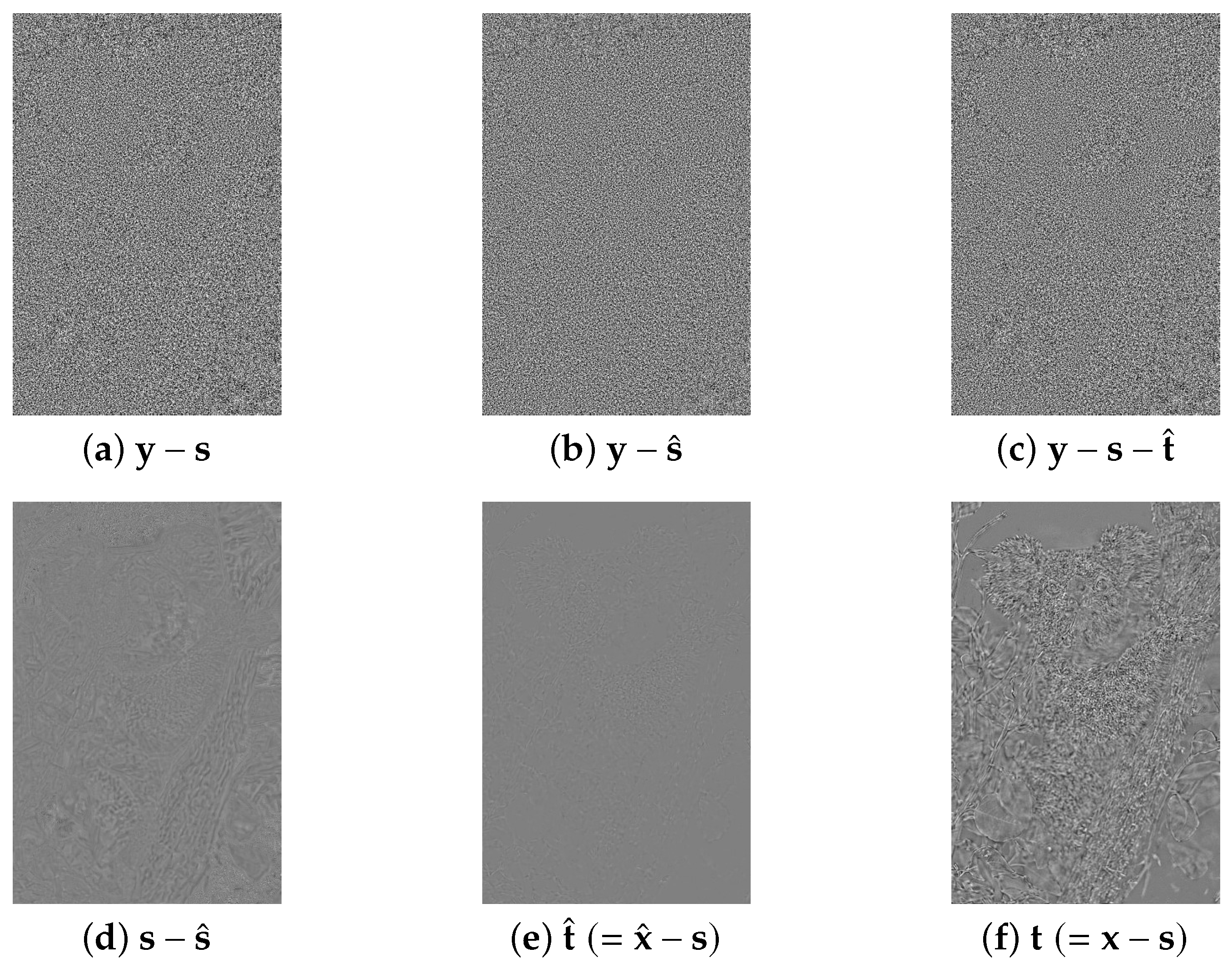
Figure A1 shows six residual images, , , , , , and (where is obtained by applying our simple linear approximation to ), which were generated for the original image ‘69015’ (shown in Figure 1) from BSD100. The noise level was set to 20. These results show that the linear approximation is almost valid since is similar to . Additionally, is similar to in strongly, moderately, and weakly textured regions such as the fur, the tree bark, and the black background, respectively.
Figure A1.
Six residual images for the image named 69015 in BSD100. To increase the visibility, each residual value is multiplied by a factor of 3.
Figure A1.
Six residual images for the image named 69015 in BSD100. To increase the visibility, each residual value is multiplied by a factor of 3.

Appendix B.3. Assumption Regarding the Estimate of the Texture Covariance Matrix
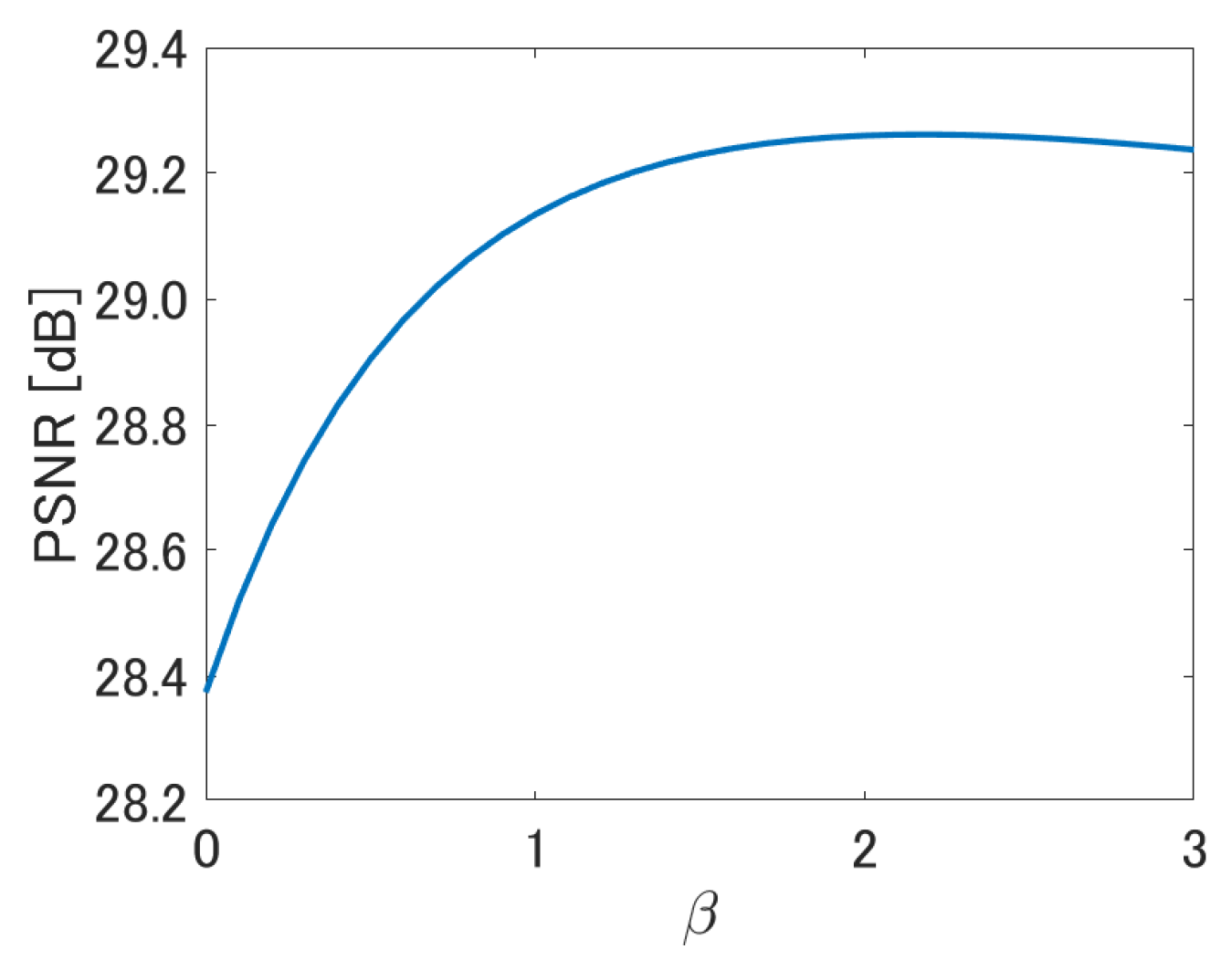
In Section 3.3, we assume that can be estimated as . We performed an experiment to experimentally prove this assumption. With some abuse of notation, we define in this subsection and experimentally confirm a relationship between the parameter and the denoising performance.
We used the 10 images of dataset I and set the noise level to 20. In this experiment, the parameter was varied in the range of 0 to 3 in increments of 0.1, and the noisy images were denoised using the proposed method with . We calculated the PSNR from all output images of the proposed method and for each . Note that this PSNR is not the average of the PSNR of each image but rather is calculated as the average of the squared error of each image. The experimental results are shown in Figure A2.
This figure shows that the denoising performance is highest when is approximately 2. Thus, we assume that .
Figure A2.
The relation ship between the parameter and the denoising performance of the proposed method when the is applied to .
Figure A2.
The relation ship between the parameter and the denoising performance of the proposed method when the is applied to .

References
- Donoho, D. De-Noising by Soft-Thresholding. IEEE Trans. Inf. Theory 1995, 41, 613–627. [Google Scholar] [CrossRef] [Green Version]
- Knaus, C.; Zwicker, M. Dual-Domain Image Denoising. In Proceedings of the 2013 IEEE International Conference on Image Processing, Melbourne, VIC, Australia, 15–18 September 2013; pp. 440–444. [Google Scholar] [CrossRef]
- Salvador, J.; Borsum, M.; Kochale, A. A Bayesian Approach for Natural Image Denoising. In Proceedings of the 2013 IEEE International Conference on Image Processing, Melbourne, VIC, Australia, 15–18 September 2013; pp. 1095–1099. [Google Scholar] [CrossRef]
- Rudin, L.I.; Osher, S.; Fatemi, E. Nonlinear Total Variation Based Noise Removal Algorithms. Phys. D Nonlinear Phenom. 1992, 60, 259–268. [Google Scholar] [CrossRef]
- Blu, T.; Luisier, F. The SURE-LET Approach to Image Denoising. IEEE Trans. Image Process. 2007, 16, 2778–2786. [Google Scholar] [CrossRef] [PubMed] [Green Version]
- Luisier, F.; Blu, T.; Unser, M. A New SURE Approach to Image Denoising: Interscale Orthonormal Wavelet Thresholding. IEEE Trans. Image Process. 2007, 16, 593–606. [Google Scholar] [CrossRef] [PubMed] [Green Version]
- Kumar, A.; Ahmad, M.O.; Swamy, M.N.S. A Framework for Image Denoising Using First and Second Order Fractional Overlapping Group Sparsity (HF-OLGS) Regularizer. IEEE Access 2019, 7, 26200–26217. [Google Scholar] [CrossRef]
- Zachevsky, I.; Zeevi, Y.Y.J. Statistics of Natural Stochastic Textures and Their Application in Image Denoising. IEEE Trans. Image Process. 2016, 25, 2130–2145. [Google Scholar] [CrossRef] [PubMed]
- Zhang, K.; Zuo, W.; Chen, Y.; Meng, D.; Zhang, L. Beyond a Gaussian Denoiser: Residual Learning of Deep CNN for Image Denoising. IEEE Trans. Image Process. 2017, 26, 3142–3155. [Google Scholar] [CrossRef] [Green Version]
- Dong, W.; Shi, G.; Li, X. Nonlocal Image Restoration With Bilateral Variance Estimation: A Low-Rank Approach. IEEE Trans. Image Process. 2013, 22, 700–711. [Google Scholar] [CrossRef] [PubMed]
- Dabov, K.; Foi, A.; Katkovnik, V.; Egiazarian, K. Image Denoising by Sparse 3-D Transform-Domain Collaborative Filtering. IEEE Trans. Image Process. 2007, 16, 2080–2095. [Google Scholar] [CrossRef]
- Chatterjee, P.; Milanfar, P. Patch-Based Near-Optimal Image Denoising. IEEE Trans. Image Process. 2012, 21, 1635–1649. [Google Scholar] [CrossRef] [PubMed]
- Pang, J.; Cheung, G. Graph Laplacian Regularization for Image Denoising: Analysis in the Continuous Domain. IEEE Trans. Image Process. 2017, 26, 1770–1785. [Google Scholar] [CrossRef] [Green Version]
- Mairal, J.; Bach, F.; Ponce, J.; Sapiro, G.; Zisserman, A. Non-Local Sparse Models for Image Restoration. In Proceedings of the IEEE International Conference on Computer Vision, Kyoto, Japan, 29 September–2 October 2009; pp. 2272–2279. [Google Scholar] [CrossRef]
- Dong, W.; Zhang, L.; Shi, G.; Li, X. Nonlocally Centralized Sparse Representation for Image Restoration. IEEE Trans. Image Process. 2013, 22, 1620–1630. [Google Scholar] [CrossRef] [PubMed] [Green Version]
- Gu, S.; Xie, Q.; Meng, D.; Zuo, W.; Feng, X.; Zhang, L. Weighted Nuclear Norm Minimization and Its Applications to Low Level Vision. Int. J. Comput. Vision 2017, 121, 183–208. [Google Scholar] [CrossRef]
- Wen, B.; Li, Y.; Bresler, Y. When Sparsity Meets Low-Rankness: Transform Learning With Non-Local Low-Rank Constraint for Image Restoration. In Proceedings of the 2017 IEEE International Conference on Acoustics, Speech and Signal Processing, New Orleans, LA, USA, 5–9 March 2017; pp. 2297–2301. [Google Scholar] [CrossRef]
- Lefkimmiatis, S. Non-Local Color Image Denoising With Convolutional Neural Networks. In Proceedings of the 2017 IEEE Conference on Computer Vision and Pattern Recognition, Honolulu, HI, USA, 21–26 July 2017; pp. 5882–5891. [Google Scholar] [CrossRef] [Green Version]
- Zuo, W.; Zhang, L.; Song, C.; Zhang, D.; Gao, H. Gradient Histogram Estimation and Preservation for Texture Enhanced Image Denoising. IEEE Trans. Image Process. 2014, 23, 2459–2472. [Google Scholar] [CrossRef] [PubMed] [Green Version]
- Zhao, W.; Liu, Q.; Lv, Y.; Qin, B. Texture Variation Adaptive Image Denoising With Nonlocal PCA. IEEE Trans. Image Process. 2019, 28, 5537–5551. [Google Scholar] [CrossRef] [PubMed]
- Liu, Z.; Yu, L.; Sun, H. Image Denoising via Nonlocal Low Rank Approximation With Local Structure Preserving. IEEE Access 2019, 7, 7117–7132. [Google Scholar] [CrossRef]
- Stein, C.M. Estimation of the Mean of a Multivariate Normal Distribution. Ann. Stat. 1981, 9, 1135–1151. [Google Scholar] [CrossRef]
- Dowson, D.; Landau, B. The Fréchet Distance Between Multivariate Normal Distributions. J. Multivar. Anal. 1982, 12, 450–455. [Google Scholar] [CrossRef] [Green Version]
- Saito, Y.; Miyata, T. Recovering Texture of Denoised Image via Its Statistical Analysis. In Proceedings of the 2018 IEEE International Conference on Image Processing, Athens, Greece, 7–10 October 2018; pp. 1767–1771. [Google Scholar] [CrossRef]
- Martin, D.; Fowlkes, C.; Tal, D.; Malik, J. A Database of Human Segmented Natural Images and Its Application to Evaluating Segmentation Algorithms and Measuring Ecological Statistics. In Proceedings of the IEEE International Conference on Computer Vision, Vancouver, BC, Canada, 7–14 July 2001; Volume 2, pp. 416–423. [Google Scholar] [CrossRef] [Green Version]
- Wang, Z.; Bovik, A.; Sheikh, H.; Simoncelli, E. Image Quality Assessment: From Error Visibility to Structural Similarity. IEEE Trans. Image Process. 2004, 13, 600–612. [Google Scholar] [CrossRef] [PubMed] [Green Version]
- Heusel, M.; Ramsauer, H.; Unterthiner, T.; Nessler, B.; Hochreiter, S. GANs Trained by a Two Time-Scale Update Rule Converge to a Local Nash Equilibrium. In Proceedings of the 31st International Conference on Neural Information Processing Systems; Curran Associates, Inc.: Red Hook, NY, USA, 2017; pp. 6629–6640. [Google Scholar]
Figure 1.
Texture is lost via image denoising.

Figure 2.
Scheme of our proposed texture recovery method. In contrast to existing image denoising methods [1,2,3,4,5,6,7,8,9,10,11,12,13,14,15,16,17,18,19,20,21], including texture-aware methods [8,19,20,21], our method recovers the texture from both the observed image and the denoised image obtained via WNNM [16].

Figure 3.
Dataset I: The ten test images from [21] used in the experiments.
Figure 3.
Dataset I: The ten test images from [21] used in the experiments.

Figure 4.
Performance comparison of GHP, WNNM, and the proposed method.

Figure 5.
True texture and estimated texture of the proposed method. The pixel value of each image is multiplied by a factor of 3.
Figure 5.
True texture and estimated texture of the proposed method. The pixel value of each image is multiplied by a factor of 3.

Figure 6.
Histogram of the values that maximize the SSIM for each output image.
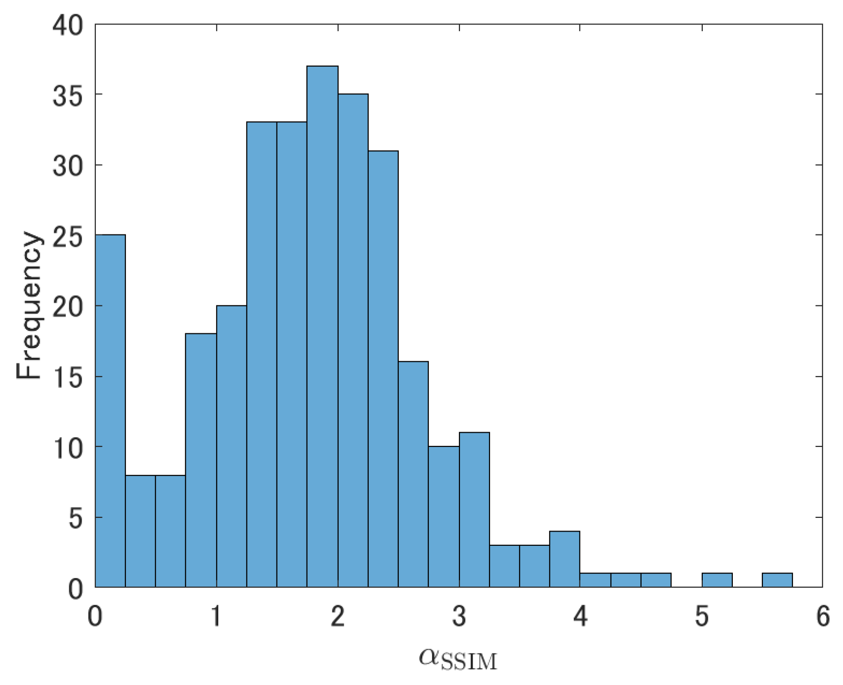
Figure 7.
Histogram of the values that maximize the PSNR for each output image.

Figure 8.
Histogram of two Fréchet distances: one calculated between the proposed estimated texture covariance matrix and the oracle sampled texture covariance matrix and the other calculated between the simply sampled estimate determined from the observation and the same oracle covariance matrix. Note that only a few of the values in these histograms lie outside of the range displayed on the x-axis.


Table 1.
The PSNR [dB] and SSIM results obtained after denoising on dataset I (with a noise standard deviation of ).
Table 1.
The PSNR [dB] and SSIM results obtained after denoising on dataset I (with a noise standard deviation of ).
| BM3D | GHP | WNNM | Proposed | |
|---|---|---|---|---|
| Image01 | 34.31/0.932 | 34.31/0.925 | 34.70/0.935 | 34.74/0.937 |
| Image02 | 32.99/0.887 | 32.97/0.884 | 33.12/0.889 | 33.23/0.896 |
| Image03 | 31.64/0.907 | 31.79/0.909 | 31.86/0.910 | 31.95/0.916 |
| Image04 | 30.58/0.898 | 30.66/0.904 | 30.76/0.900 | 30.80/0.905 |
| Image05 | 32.59/0.946 | 32.52/0.932 | 32.88/0.948 | 32.89/0.949 |
| Image06 | 33.61/0.917 | 33.61/0.905 | 33.90/0.921 | 33.99/0.925 |
| Image07 | 34.19/0.898 | 34.11/0.894 | 34.41/0.902 | 34.48/0.906 |
| Image08 | 31.48/0.908 | 31.51/0.907 | 31.73/0.912 | 31.80/0.917 |
| Image09 | 35.12/0.946 | 34.96/0.934 | 35.30/0.946 | 35.35/0.948 |
| Image10 | 31.71/0.912 | 31.76/0.907 | 31.84/0.913 | 31.92/0.917 |
| Average | 32.82/0.915 | 32.82/0.910 | 33.05/0.918 | 33.11/0.922 |
Table 2.
The PSNR [dB] and SSIM results obtained after denoising on dataset I (with a noise standard deviation of ).
Table 2.
The PSNR [dB] and SSIM results obtained after denoising on dataset I (with a noise standard deviation of ).
| BM3D | GHP | WNNM | Proposed | |
|---|---|---|---|---|
| Image01 | 30.47/0.868 | 30.58/0.869 | 30.81/0.872 | 30.91/0.875 |
| Image02 | 29.55/0.765 | 29.67/0.778 | 29.64/0.765 | 29.77/0.777 |
| Image03 | 27.82/0.796 | 28.10/0.816 | 28.06/0.802 | 28.21/0.815 |
| Image04 | 26.61/0.793 | 26.74/0.803 | 26.80/0.798 | 26.91/0.809 |
| Image05 | 28.30/0.881 | 28.48/0.884 | 28.58/0.883 | 28.70/0.888 |
| Image06 | 29.96/0.828 | 30.21/0.841 | 30.25/0.833 | 30.38/0.841 |
| Image07 | 30.97/0.812 | 31.00/0.816 | 31.03/0.811 | 31.11/0.817 |
| Image08 | 27.22/0.806 | 27.41/0.818 | 27.54/0.815 | 27.69/0.827 |
| Image09 | 31.35/0.895 | 31.39/0.896 | 31.52/0.895 | 31.60/0.896 |
| Image10 | 27.82/0.803 | 27.98/0.813 | 27.96/0.807 | 28.11/0.819 |
| Average | 29.01/0.825 | 29.16/0.833 | 29.22/0.828 | 29.34/0.837 |
Table 3.
The PSNR [dB] and SSIM results obtained after denoising on dataset I (with a noise standard deviation of ).
Table 3.
The PSNR [dB] and SSIM results obtained after denoising on dataset I (with a noise standard deviation of ).
| BM3D | GHP | WNNM | Proposed | |
|---|---|---|---|---|
| Image01 | 28.51/0.817 | 28.57/0.818 | 28.75/0.822 | 28.83/0.824 |
| Image02 | 28.03/0.688 | 28.03/0.700 | 28.07/0.684 | 28.13/0.694 |
| Image03 | 26.08/0.719 | 26.21/0.738 | 26.29/0.727 | 26.39/0.740 |
| Image04 | 24.57/0.703 | 24.68/0.718 | 24.81/0.714 | 24.92/0.729 |
| Image05 | 26.04/0.813 | 26.28/0.819 | 26.38/0.823 | 26.51/0.831 |
| Image06 | 28.22/0.762 | 28.43/0.778 | 28.50/0.770 | 28.59/0.776 |
| Image07 | 29.37/0.756 | 29.24/0.757 | 29.43/0.755 | 29.45/0.759 |
| Image08 | 25.13/0.724 | 25.34/0.744 | 25.46/0.738 | 25.60/0.751 |
| Image09 | 29.48/0.854 | 29.47/0.855 | 29.65/0.856 | 29.70/0.855 |
| Image10 | 26.00/0.718 | 26.09/0.733 | 26.14/0.725 | 26.25/0.738 |
| Average | 27.14/0.755 | 27.24/0.766 | 27.35/0.761 | 27.44/0.770 |
Table 4.
The PSNR [dB] and SSIM results obtained after denoising on BSD100. The p-values were calculated by one-tailed paired t-tests on the difference of each PSNR and SSIM between the proposed method and WNNM.
Table 4.
The PSNR [dB] and SSIM results obtained after denoising on BSD100. The p-values were calculated by one-tailed paired t-tests on the difference of each PSNR and SSIM between the proposed method and WNNM.
| BM3D | GHP | WNNM | Proposed | p-Value | |
|---|---|---|---|---|---|
| 33.13/0.913 | 33.10/0.911 | 33.36/0.916 | 33.42/0.920 | / | |
| 29.42/0.824 | 29.49/0.832 | 29.64/0.829 | 29.74/0.837 | / | |
| 27.56/0.759 | 27.58/0.769 | 27.78/0.766 | 27.84/0.773 | / | |
| Average | 30.03/0.832 | 30.06/0.837 | 30.26/0.837 | 30.33/0.843 | – |
Table 5.
The averages of computational time (in seconds) of WNNM and the proposed method.
| WNNM | Proposed (WNNM + Texture Recovery) | |
|---|---|---|
| 149 | 169 | |
| 148 | 167 | |
| 311 | 334 |
Table 6.
Comparison of non-learning-based methods (WNNM and the proposed method) and a learning-based method (DnCNN). The PSNR [dB] and SSIM results obtained after denoising on dataset I (with a noise standard deviation of ). Note that the proposed method does not require any training and is fully explainable. The bold value means the highest PSNR or SSIM in non-learning-based methods.
| WNNM | Proposed | DnCNN | |
|---|---|---|---|
| Image01 | 32.38/0.902 | 32.45/0.905 | 32.70/0.911 |
| Image02 | 31.00/0.824 | 31.13/0.834 | 31.38/0.845 |
| Image03 | 29.53/0.853 | 29.67/0.864 | 29.89/0.872 |
| Image04 | 28.37/0.847 | 28.45/0.856 | 28.59/0.860 |
| Image05 | 30.30/0.916 | 30.37/0.919 | 30.53/0.922 |
| Image06 | 31.69/0.876 | 31.81/0.882 | 31.82/0.886 |
| Image07 | 32.37/0.852 | 32.45/0.858 | 32.68/0.867 |
| Image08 | 29.20/0.862 | 29.32/0.871 | 29.58/0.877 |
| Image09 | 33.00/0.919 | 33.08/0.921 | 33.35/0.927 |
| Image10 | 29.47/0.858 | 29.60/0.867 | 29.79/0.874 |
| Average | 30.73/0.871 | 30.83/0.878 | 31.03/0.884 |
Publisher’s Note: MDPI stays neutral with regard to jurisdictional claims in published maps and institutional affiliations. |
© 2021 by the authors. Licensee MDPI, Basel, Switzerland. This article is an open access article distributed under the terms and conditions of the Creative Commons Attribution (CC BY) license (https://creativecommons.org/licenses/by/4.0/).
Share and Cite
MDPI and ACS Style
Saito, Y.; Miyata, T. Recovering Texture with a Denoising-Process-Aware LMMSE Filter. Signals 2021, 2, 286-303. https://doi.org/10.3390/signals2020019
AMA Style
Saito Y, Miyata T. Recovering Texture with a Denoising-Process-Aware LMMSE Filter. Signals. 2021; 2(2):286-303. https://doi.org/10.3390/signals2020019
Chicago/Turabian StyleSaito, Yuta, and Takamichi Miyata. 2021. "Recovering Texture with a Denoising-Process-Aware LMMSE Filter" Signals 2, no. 2: 286-303. https://doi.org/10.3390/signals2020019