Article

On the Synergy between Nonconvex Extensions of the Tensor Nuclear Norm for Tensor Recovery

1
Chiba Institute of Technology, Narashino-shi 275-0016, Japan
2
Department of Computer Science, School of Computing, Tokyo Institute of Technology, Meguro-ku 152-8552, Japan
*
Author to whom correspondence should be addressed.
Signals 2021, 2(1), 108-121; https://doi.org/10.3390/signals2010010
Submission received: 30 September 2020 / Revised: 14 December 2020 / Accepted: 1 February 2021 / Published: 18 February 2021

Abstract

:
Low-rank tensor recovery has attracted much attention among various tensor recovery approaches. A tensor rank has several definitions, unlike the matrix rank—e.g., the CP rank and the Tucker rank. Many low-rank tensor recovery methods are focused on the Tucker rank. Since the Tucker rank is nonconvex and discontinuous, many relaxations of the Tucker rank have been proposed, e.g., the sum of nuclear norm, weighted tensor nuclear norm, and weighted tensor schatten-p norm. In particular, the weighted tensor schatten-p norm has two parameters, the weight and p, and the sum of nuclear norm and weighted tensor nuclear norm are special cases of these parameters. However, there has been no detailed discussion of whether the effects of the weighting and p are synergistic. In this paper, we propose a novel low-rank tensor completion model using the weighted tensor schatten-p norm to reveal the relationships between the weight and p. To clarify whether complex methods such as the weighted tensor schatten-p norm are necessary, we compare them with a simple method using rank-constrained minimization. It was found that the simple methods did not outperform the complex methods unless the rank of the original tensor could be accurately known. If we can obtain the ideal weight, p = 1 is sufficient, although it is necessary to set p < 1 when using the weights obtained from observations. These results are consistent with existing reports.

1. Introduction

A tensor is a powerful tool that can describe multidimensional information and the complex relationships among elements, and it is widely used in the field of signal and image processing [1,2,3,4,5,6,7,8,9,10,11,12]. Usually, such information cannot be fully obtained through observation, and we need to complete or recover a full tensor from incomplete or degraded measurements, which are corrupted by noise, missing entries, and/or outliers. Among various tensor completion/recovery approaches, low-rank-based methods have attracted much attention because they exploit the essential structure of tensors and achieve accurate estimation.
Unlike the matrix rank, there are several different definitions of the tensor rank; well-known examples include the CANDECOMP/PARAFAC (CP) rank [13] and the Tucker rank [14]. Since determining the CP rank is NP-hard [15], many existing low-rank tensor recovery methods are focused on the Tucker rank. The Tucker rank is defined as follows: (1) an input tensor is converted to the matrices (by the unfolding operation); (2) the average rank of these matrices is calculated. The Tucker rank is very difficult to handle because of its nonconvexity and discontinuity.
To address this problem, the sum of nuclear norm, which is a convex surrogate of the Tucker rank, is proposed [1,3]. Methods based on the Tucker rank replace the rank of unfolding matrices with their nuclear norms, where the nuclear norm is known as a continuous tightest convex surrogate of the matrix rank [16].
On the other hand, the weighted nuclear norm and the schatten-p norm have been proposed as different surrogates of the matrix rank [17,18,19,20]. Both are a generalization of the nuclear norm and usually perform better than the nuclear norm for low-rank matrix recovery. Following this trend, a weighted tensor nuclear norm and a tensor schatten-p norm have also been proposed [11,12]. They are extensions of the weighted nuclear norm and the schatten-p norm for tensors, respectively, and they generally perform better for low-rank tensor recovery as well. However, for effective use, we need to select appropriate weights and parameters p.
The ideal (oracle) weights for the weighted nuclear norm are the inverses of the singular values of the original matrix. This is because the weighted nuclear norm with the oracle weights of the original matrix is identical to the rank. Generally, obtaining the singular values of the original matrix is difficult. Therefore, for practical usage, we need some methods to estimate the singular values of the original matrix to determine the weights [19]. On the other hand, the parameter p for the schatten-p norm is generally determined in a heuristic manner and, in most cases, p < 1 is employed [8,12,18]. We should note that both the weighted tensor nuclear norm and the tensor schatten-p norm (with p < 1 ) are in general nonconvex, as is the case with the matrix counterparts.
Now, some natural questions arise: Are the effects of the weightings for singular values and the schatten-p extension synergistic, or does one of them encompass? Is there any chance that a simple rank-constrained minimization, which is also a nonconvex optimization, can compete with these advanced and complicated methods?
In this paper, to answer the questions above, we propose a novel general constrained optimization problem combining the weighting and the schatten-p extension for tensors, and we develop an efficient algorithm to solve it. We performed exhaustive experiments, and the results showed that, if we can use the oracle weights, the combination of p = 1 and the weighting is the most effective choice for all cases. We also found that the combination of p = 1 / 2 and the weighting is effective when using the weights estimated from degraded measurements. The rank-constrained minimization problem performs well as long as we know the rank of the original tensor. If we are agnostic toward the correct rank, the performance drops sharply.
The main contributions of this paper are summarized as follows:
  • We propose a general constrained optimization problem and an efficient solver for analyzing the relationship between the weightings of singular values and the schatten-p extension for tensors.
  • We show that the weighting and the schatten-p extension are synergetic and that the effective value of p is dependent on how the weights are determined.
  • We show that the rank constrained minimization problem is not able to outperform the advanced methods unless the true rank of the original tensor is known. The performance is sensitive to the rank values used as the constraints.

2. Low-Rank Tensor Completion

In what follows, N , R , and R + denote the set of all nonnegative integers, all real numbers, and all nonnegative real numbers. We use capital calligraphic letters for tensors, capital bold letters for matrices, and lowercase bold letters for column vectors.
In this paper, we assume that an observation model of tensor recovery can be described as
Y = A Ω ( X org + V ) ,
where Y R n 1 × × n N , X org R n 1 × × n N , and V R n 1 × × n N are an Nth order observation tensor, an Nth order low-rank original tensor, and an Nth order random tensor, respectively, whose entries are independent and identically distributed Gaussian variables with zero mean and known variance σ n 2 .
The degradation operator is defined as
A Ω ( X ) i 1 , , i N = X i 1 , , i N ( i 1 , , i N Ω ) 0 ( otherwise ) ,
where Ω is a set of indicators of observable entries.
If we can assume that the original tensor is low rank, it can be estimated by finding a tensor that is close to the observation tensor and also low rank. In particular, assuming that the rank of the original tensor is known and that the variance of the noise is 0, estimating the original tensor is the problem of finding a tensor whose rank is identical to the rank of the original tensor and whose known elements match the observation tensor, i.e., finding a tensor within the following set:
Find X R n 1 × × n N s . t . A Ω ( X ) = A Ω ( Y ) , rank m ( X ) = r ^ m
where rank m ( X ) = rank ( unfold m ( X ) ) and m = 1 , , N . We denote rank as the matrix rank and r ^ m as the matrix rank of an mth mode unfolded original tensor.
However, in general, the set containing the equations for the ranks, as in Equation (3), is hard to determine. Thus, we employ an alternative set with an inequality constraint instead of Equation (3):
Find X R n 1 × × n N s . t . A Ω ( X ) = A Ω ( Y ) , rank m ( X ) r ^ m ,
The sets shown in Equations (3) and (4) are used directly for the estimation of the original tensor because they generally contain multiple matrices. Additionally, if the observation process includes noise ( σ N 0 ), it may yield the empty set. Thus, we employ the L2 norm between the observation tensor, which corresponds to the negative log-likelihood of the Gaussian distribution, and the solution of the following minimization problem, including this norm as the estimated tensor:
min X R n 1 × × n N A Ω ( X ) Y 2 2 s . t . rank m ( X ) r ^ m ( m = 1 , , N ) ,
where · 2 is an 2 norm of the tensor that is defined as the square root of the sum of the squares of each element of the tensor. Although this problem is one of nonconvex optimization, we can efficiently solve it by using the alternating direction method of multipliers (ADMM) [21], which is known as an algorithm for solving convex optimization problems and is effective in practice for solving nonconvex optimization problems [22,23,24]. A detail of an algorithm to solve Equation (5) explains in Appendix A.
Equations (3) and (5) include the matrix rank of each unfolded tensor, which is very difficult to handle since it is not only nonconvex but also discontinuous. Moreover, the situation in which we know the rank of each unfolded matrix of the original tensor r ^ m is unrealistic.
The weighted tensor schatten-p norm (WTSPN) is proposed as a representation of a nonconvex but continuous tensor rank,
· w , γ , p : R n 1 × × n N R + : X m = 1 N γ m unfold m ( X ) w m , p p ,
where · w , p p is a weighted schatten-p norm raised to the power p (WSPN) [20]; w = [ w 1 , , w N ] is the weight vector of the WSPNs; γ m is a positive constant satisfying m = 1 N γ m = 1 ; γ = [ γ 1 , , γ N ] , and unfold ( · ) is an unfolding operator.
The WTSPN is generally a nonconvex function that is consistent with the weighted tensor nuclear norm [11] when p = 1 , the tensor schatten-p norm [12] when w is uniform (all elements of w are the same value), and the sum of nuclear norm [1,3] when p = 1 and w is uniform.
The mth mode tensor unfolding operator of the nth order tensor unfold m : R n 1 × × n N R n m × I m is defined as a map from the tensor elements ( i 1 , , i N ) to the corresponding matrix elements ( i m , j m ), where I m = k = 1 k m N i k ,
j m = 1 + k = 1 k m N ( i k 1 ) l = 1 l m k 1 i l .
The WSPN is described as
· w , p p : R n v × n h R + : X k = 1 n m w k σ k ( X ) p ,
where 0 < p , n m = min ( n v , n h ) , σ k ( X ) R + ( k = 1 , , n m ) is the kth largest singular value of X , and w = [ w 1 , , w n m ] R + n m is a weight vector that satisfies 0 w 1 w 2 w n m . The WSPN is a generalization of the nuclear norm and the weighted nuclear norm [17,19], which are often used in low-rank matrix recovery.
As mentioned in Section 1, the proper weights of the WTSPN and the proper value of p have not been investigated in detail. Revealing them is one of the objectives of this paper.
On the other hand, when recovering the observation model of Equation (1) with the WTSPN as the regularization term and the 2 norm as the fidelity term, even if the noise variance does not change, the optimal hyperparameter (balancing the regularization term and the fidelity term) varies according to the parameters of the regularization term, w , and p. This makes a fair comparison difficult. In addition, a parameter that is so difficult to tune is not desirable for practical use. Therefore, in the next section, we propose a method to solve this problem.

3. Proposed Method

To solve the above problem, we propose a method using 2 ball constraints and WTSPN minimization. Specifically, we formulate the following minimization problem:
min X X w , γ , p s . t . A Ω ( X ) B ( Y , σ n | Ω | ) ,
where B ( Y , r ) is an 2 ball, and the 2 ball with center Y R n 1 × × n N and radius r R is defined as
B ( Y , r ) : = { X R n 1 × × n N | X Y 2 r } .
By using the ball constraint, it is possible to determine the appropriate parameters based only on the variance of the noise [25,26,27], which is convenient when comparing various regularization parameters, as in this paper. Additionally, | Ω | is the number of elements of the set Ω .
Since we assume that the standard deviation of noise σ n is known, we can expect the realization of the noise V added to the original tensor to exist inside the hypersphere determined by the standard deviation. The constraints of Equation (9) are in accordance with this fact. This method allows us to “fairly compare the performance of different regularization terms (if the variance of the noise is known)”.
In general, Equation (9) is a nonconvex optimization problem, which makes it difficult to find a globally optimal solution. As mentioned in Section 2, ADMM exhibits empirical performance on nonconvex optimization problems. Therefore, we propose solving Equation (9) using ADMM. The proposed algorithm is shown in Algorithm 1.
The objective function in line 5 of Algorithm 1 is
argmin X X λ γ m w m , p p + 1 2 unfold m ( X ( k + 1 ) ) + Z 1 , m ( k ) X F 2
which is nonconvex, although one of the solutions can be written as [8,18,20]:
U S λ γ m w m , p ( Σ ) V ,
where U Σ V = unfold m ( X ( k + 1 ) ) + Z 1 , m ( k ) is a singular value decomposition (SVD) and S w , p ( · ) is a weighted thresholding operator.
Algorithm 1 Proposed algorithm
Input: Y , σ n , γ = [ γ 1 , , γ N ] , w = [ w 1 , , w N ] , p, λ
1: Initialize Y 1 , m ( 0 ) = unfold m ( Y ) , Y 2 ( 0 ) = Y , Z 1 , m ( 0 ) = 0 , Y 1 , m ( 0 ) , Z 2 ( 0 ) = 0
2: while A stopping criterion is not satisfied do
3:   X ( k + 1 ) = argmin X 1 2 m = 1 N Y 1 , m ( k ) unfold m ( X ) Z 1 , m ( k ) 2 2 + λ Y 2 ( k ) A Ω ( X ) Z 2 ( k ) 2 2
4:  for m = 1 to N do
5:    Y 1 , m ( k + 1 ) = argmin X X λ γ m w m , p p + 1 2 unfold m ( X ( k + 1 ) ) + Z 1 , m ( k ) X F 2
6:    Z 1 , m ( k + 1 ) = Z 1 , m ( k ) + unfold m ( X ( k + 1 ) ) Y 1 , m ( k + 1 )
7:  end for
8:   Y 2 ( k + 1 ) = proj B ( Y , σ n | ω | ) ( A Ω ( X ( k + 1 ) + Z 2 ( k ) ) ) + A Ω ¯ ( X ( k + 1 ) + Z 2 ( k ) )
9:   Z 2 ( k + 1 ) = Z 2 ( k ) + A Ω ( X ( k + 1 ) ) Y 2 ( k + 1 )
10:   λ = 0.99 λ
11:   k = k + 1
12: end while
Output: X ( k )
Each element of the weighted thresholding operator for a rectangular diagonal matrix Y ( S w , p ( Y ) ) i , i is defined as a solution to the following minimization problem:
argmin x 1 2 ( Y i , i x ) 2 + w i | x | p .
The solution of Equation (13) is a soft thresholding max ( Y i , i w i , 0 ) when p = 1 and the closed-form thresholding proposed in [28] when p = { 1 / 2 , 2 / 3 } .
The first term in line 8 of Algorithm 1 is
proj B ( Y , σ n | Ω | ) ( A Ω ( X ( k + 1 ) + Z 2 ( k ) ) )
which is a metric projection of the set B ( Y , σ n | Ω | ) . The metric projection is defined as
proj S : R N R N : x argmin y S 1 2 x y 2 2 .
Equation (14) has a closed-form solution,
Y min σ n | Ω | Y A Ω ( X ( k + 1 ) + Z 2 ( k ) ) 2 , 1 ( Y A Ω ( X ( k + 1 ) + Z 2 ( k ) ) ) .
The set of Ω ¯ in the second term of line 8,
A Ω ¯ ( X ( k + 1 ) + Z 2 ( k ) )
is the complement of the set Ω , which is a set of indicators of missing entries. A Ω ¯ is defined as
A Ω ¯ ( X ) i 1 , , i N = X i 1 , , i N ( i 1 , , i N Ω ¯ ) 0 ( otherwise ) .

4. Experimental Comparison

4.1. Setting

In Section 1, we posed two questions:
  • Are the effects of the weighting and p-squared on singular values synergistic? Or does one encompass the other?
  • Is simple rank-constrained minimization insufficient?
To answer these questions, we performed some experiments using an artificial tensor. Each element of an Nth order artificial tensor X R n 1 × × n N is generated by using the Tucker model:
X ( i 1 , , i N ) = 1 j 1 r 1 , , 1 j N r N S ( j 1 , , j N ) k N U k ( i k , j k ) ,
where [ r 1 , , r N ] , S R r 1 × × r N and U k R n k × r k are the matrix ranks of unfold m ( X ) ( m = 1 , , N ) , the core tensor, and the factor tensor. Each element of S and U k is generated uniformly over the intervals [ 0 , 1 ] and [ 0.5 , 0.5 ] , respectively. Finally, we normalized the difference between the maximum and minimum elements of X to 1.
As mentioned in Section 1, the widely used weights used as the ideal weights for the singular values are the inverses of the singular values of the unfolded original tensor X org . Throughout this paper, we define our ideal weights as
( w Id ( α ) ) i , j = R σ i ( unfold j ( X org ) ) α k σ k ( unfold j ( X org ) ) α ,
where R is the smaller of the row and column dimensions of unfold j ( X org ) . Since the ideal weights are not always optimal in terms of the recovery performance, we introduce a parameter α to bring additional flexibility to the setting of the weights. However, the true singular values are not available in practical applications.
A method that does not require the true singular values is to use the singular values obtained from observations for estimating the ideal weights. One of these methods is as follows:
( w Obs ( α ) ) i , j = R σ i ( unfold j ( Y ˜ ) ) α k σ k ( unfold j ( Y ˜ ) ) α
where Y ˜ is a tensor the missing elements of the observation tensor Y filled in using the average of the observed entries of the observation tensor Y . We refer to these weights as observation weights.
The tensor schatten-p norm with no weights is a special case of the WTSPN. Therefore, we can use the WTSPN with the following special weights as the tensor schatten-p norm:
( w Uni ) i , j = 1 .
In the following experiments, we use three types of weights (the ideal weights w Id , observation weights w Obs and uniform weights w Uni ) to reveal the relationship between the weighting and schatten-p extension on the performance of WTSPN. The weight determination parameter α varies in increments of 0.25 in the range [ 1 , 4 ] . The parameters of schatten-p are chosen from p = { 1 / 2 , 2 / 3 , 1 } , and each element of γ is set to 1 / N , where N is the order of the target tensor. In all cases, the parameter of ADMM is set to λ = 100 .
We compare the performance of Algorithm 1 using w Id , w Obs , and w Uni as well as rank-constrained minimization. The following error is used to evaluate the performance of each method:
error ( X ˜ , Y ) = 1 m = 1 N I m X ˜ Y 2 ,
where X ˜ is the estimated tensor obtained by each method.

4.2. Results and Discussion

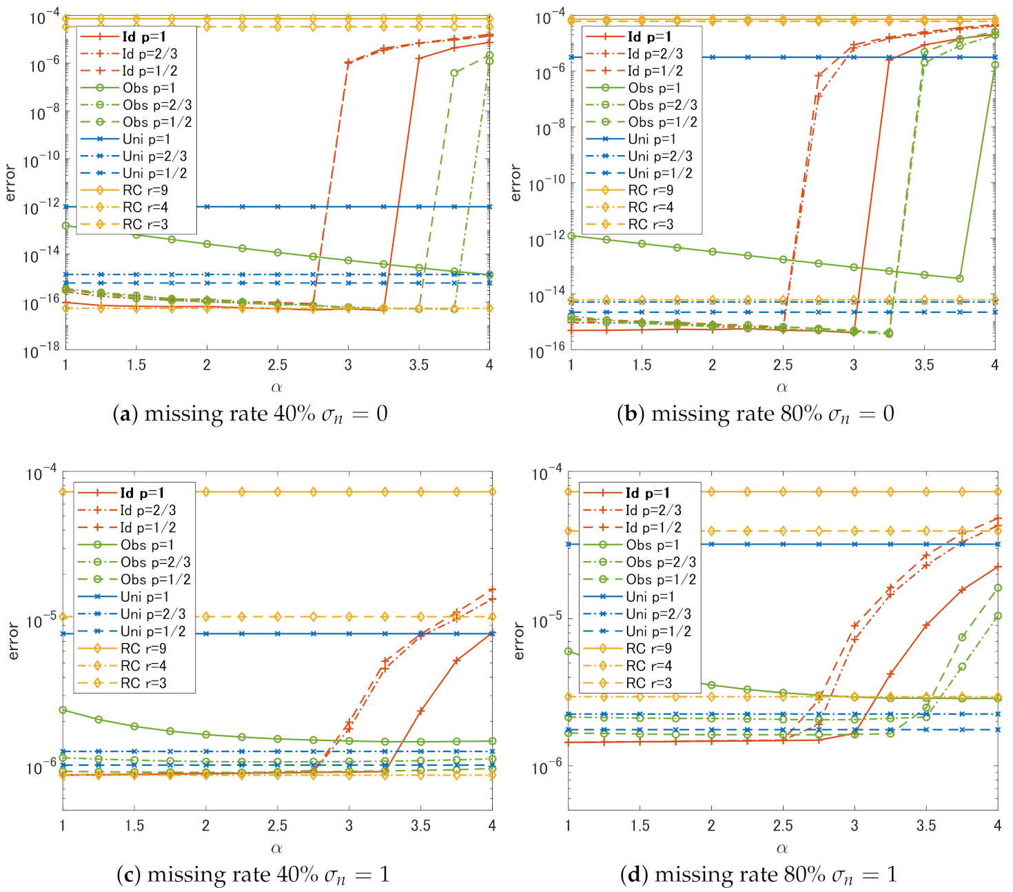
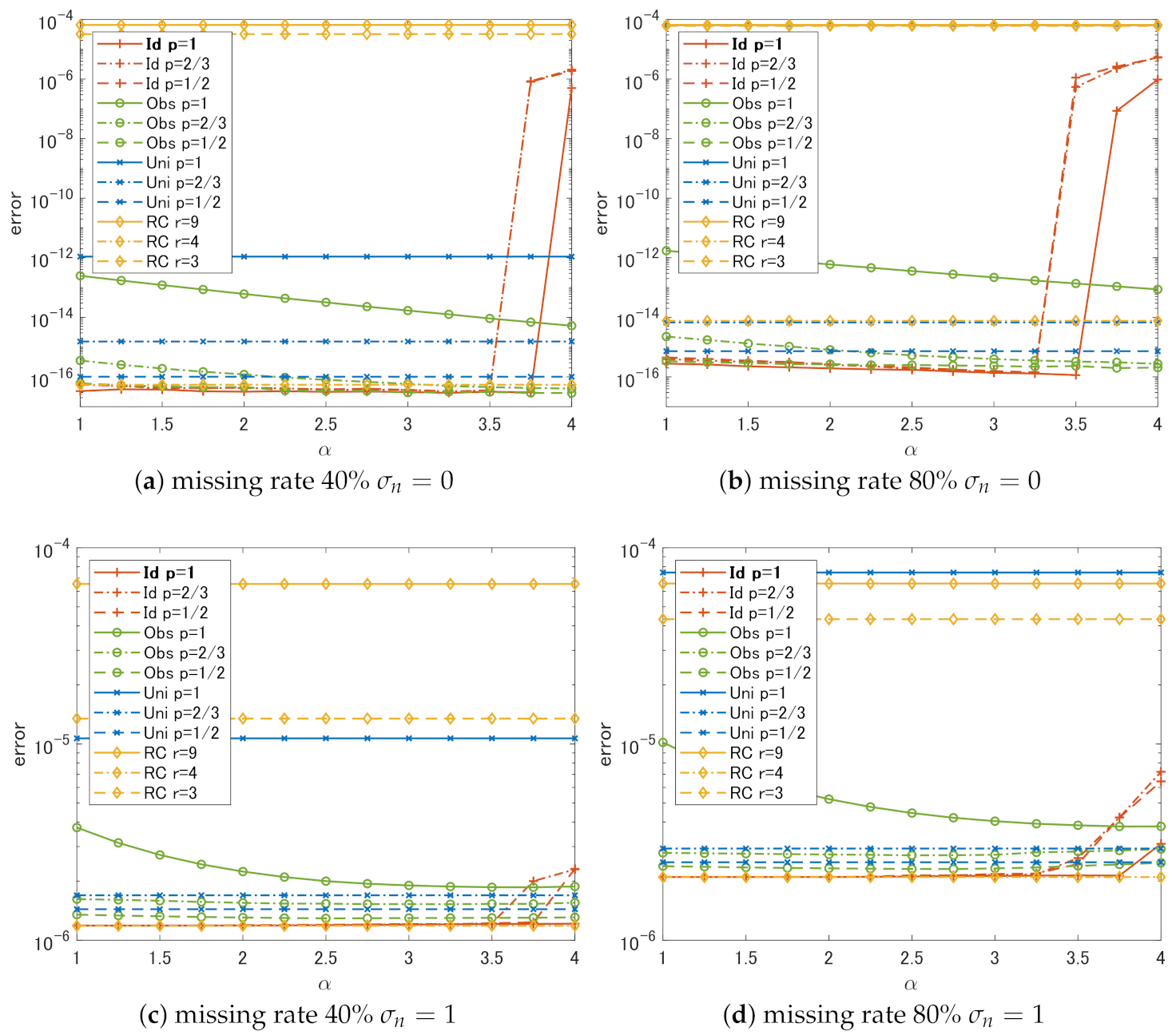
We performed recovery from observed tensors with missing rate of 0.4 and 0.8 and standard deviations of noise σ n of 0 and 1, and the results of the combinations of these parameters are shown in (a) to (d) in Figure 1, Figure 2, Figure 3 and Figure 4. The horizontal axis of each graph is the parameter α used in Equations (20) and (21) for determining the weights, and the vertical axis is the performance of each method defined by Equation (23). The red, green, blue, and yellow lines show the results of Algorithm 1 with w Id (Id in the legends of the graphs), with w Obs (Obs), with w Uni (Uni), and with the rank-constrained minimization shown in Equation (5) (RC). In the case of Id, Obs, and Uni, the results corresponding to the different values of p are shown with different line types. Similarly, in the case of RC, the results corresponding to the different target ranks r are shown with different line types.
Figure 1 is the result when the size of the original tensor is 40 × 40 × 40 and the rank is [ 4 , 4 , 4 ] . From the graphs (a)–(d) in Figure 1, one can see that
  • In the case of Id, if we choose α < 2 , the choice of p does not have much effect on the performance. The slowest degradation of performance due to the change in α is obtained at p = 1 .
  • In the case of Obs, p = 1 / 2 shows the best result across (a)–(d). These results are consistent with the results in previous studies [8,12,18,20].
  • Regardless of p, the performance of Id and Obs is the same or better than that of Uni in all cases.
  • In all cases, RC shows the worst performance unless we can choose the correct rank r.
Figure 2 shows the results when we only change the tensor rank to [ 5 , 5 , 5 ] . Note that the size of the tensor is still 40 × 40 × 40 . The results show a similar trend as in the case of Figure 1. From the results in Figure 1 and Figure 2, for the third-order tensor, we can conclude that the effect of the choice of the weights, p, and the algorithms on performance is rank-independent.
To reveal the impact of the changes in the order of the tensor on the common trend in Figure 1 and Figure 2, we performed experiments on the 4th-order tensor. The results are shown in Figure 3 and Figure 4. In Figure 3 and Figure 4, the sizes of the original tensors are both 16 × 16 × 16 × 16 , and the ranks are [2, 2, 2, 2] and [3, 3, 3, 3], respectively. In the case of the 4th-order tensor, there was no change in the common trend of each graph when the rank was varied. The same trend is observed in comparison with Figure 1 and Figure 2. From these observations, we can say that the relationship between the weighting and schatten-p extension and the performance gap between the proposed algorithm and the rank-constrained minimization that we revealed is a law and is independent of the tensor rank and order.
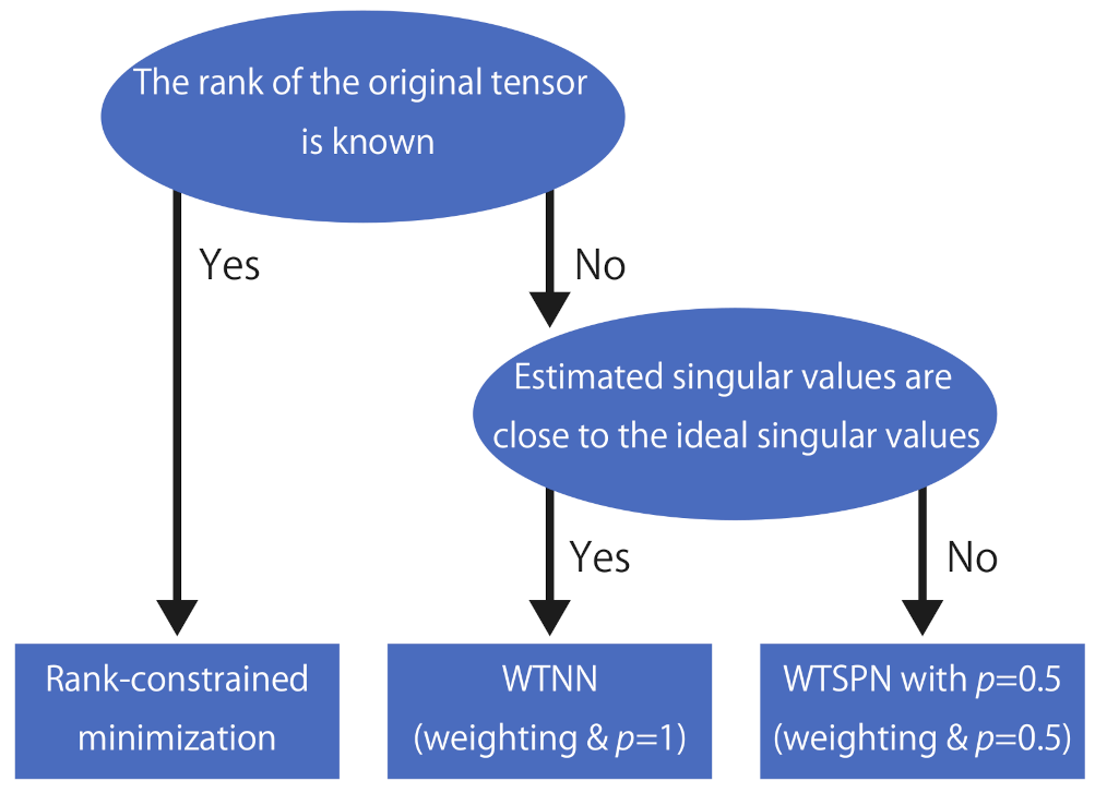
From these results, we can conclude that
  • It is sufficient to use p = 1 if weights that are close to the ideal weights can be estimated in some way.
  • It is better to set a small p-value if the weights estimated from the degraded singular values are not reliable.
  • Simple methods using rank constraints are very sensitive to the choice of ranks used for the constraints and cannot outperform complex methods like the proposed algorithm unless one can correctly estimate the original ranks.

5. Conclusions

In this paper, to reveal the relationships between the weighting and schatten-p extension, we propose a general tensor recovery model that combines them and propose an algorithm to solve it. From the experiments with artificial data using the proposed algorithms, the effect of the recovery performance in the presence or absence of the weighting and the schatten-p extension for various situations is determined.
Consequently, the simple rank-constrained minimization method cannot outperform complex methods such as the proposed algorithm unless the rank r used in the constraint is chosen properly. The relationships between the weighting and schatten-p extension in WTSPNs vary with the degree to which we can estimate the ideal weights. The schatten-p extension does not affect the performance if the ideal weight is available. On the other hand, the effect of the schatten-p and the weighting on singular values is synergistic if we need to determine the weights from heavily degraded observations.
Our conclusion is summarized in the flowchart in Figure 5, where “weighting” indicates that using the weights w , which are determined based on the estimates of the singular values of the unfolded original tensor. This flowchart implies that, if we can access limited information about the rank (or the singular values) of the original tensor, we need to use complex methods to obtain good results.
The proposed tensor restoration model was based on the observation model of Equation (1). Therefore, the proposed guideline is not applicable to problems that can not be represented in the current observation model, e.g., a multiplicative noise. We will solve this problem and validate the relationships between the weighting and the schatten-p extension in various situations in our future work.

Author Contributions

Conceptualization, K.H., S.O., and T.M.; methodology, K.H., S.O., and T.M.; software, K.H.; validation, K.H., S.O., and T.M.; formal analysis, K.H. and S.O.; investigation, K.H. and S.O.; resources, T.M.; data curation, K.H.; writing—original draft preparation, K.H.; writing —review and editing, S.O. and T.M; visualization, K.H.; supervision, T.M.; project administration, S.O. and T.M; funding acquisition, T.M. All authors have read and agreed to the published version of the manuscript.

Funding

This research was funded by the Japan Society for the Promotion of Science KAKENHI Grant No. JP19K04377.

Conflicts of Interest

The funders had no role in the design of the study; in the collection, analyses, or interpretation of data; in the writing of the manuscript, or in the decision to publish the results.

Appendix A. Algorithm for Rank-Constrained Minimization

In Section 2, we mentioned that we can solve Equation (5) efficiently by using ADMM, although we did not show a specific algorithm. The algorithm for solving Equation (5) is shown in Algorithm A1.
The objective function in line 5 of Algorithm A1 is
proj { X | rank ( X ) r ^ m } ( unfold m ( X ( k + 1 ) ) + Z 1 , m ( k ) ) ,
which is a nonconvex function because the set { X | rank ( X ) r ^ m } is a nonconvex set. However, one of the solutions of Equation (A1) can be obtained as
U T r ^ m ( Σ ) V ,
where U Σ V = unfold m ( X ( k + 1 ) ) + Z 1 , m ( k ) is an SVD and T r ^ m ( · ) is a truncation operator. The truncation operator for a rectangular diagonal matrix Y T r ( Y ) is defined as
T r ( Y ) i , i = Y i , i ( i r ) 0 ( otherwise ) .
Algorithm A1 Algorithm for rank-constrained minimization
Input: Y , λ , r 1 , , r N
1: Initialize Y 1 , m ( 0 ) = unfold m ( Y ) , Y 2 ( 0 ) = Y , Z 1 , m ( 0 ) = 0 , Y 1 , m ( 0 ) , Z 2 ( 0 ) = 0
2: while A stopping criterion is not satisfied do
3:     X ( k + 1 ) = argmin X 1 2 m = 1 N Y 1 , m ( k ) unfold m ( X ) Z 1 , m ( k ) 2 2 + λ Y 2 ( k ) A Ω ( X ) Z 2 ( k ) 2 2
4:    for m = 1 to N do
5:       Y 1 , m ( k + 1 ) = proj { X | rank ( X ) r ^ m } ( unfold m ( X ( k + 1 ) ) + Z 1 , m ( k ) )
6:       Z 1 , m ( k + 1 ) = Z 1 , m ( k ) + unfold m ( X ( k + 1 ) ) Y 1 , m ( k + 1 )
7:    end for
8:     Y 2 ( k + 1 ) = argmin X λ A Ω ( X ) Y 2 2 + 1 2 X ( k + 1 ) + Z 2 ( k ) X F 2
9:     Z 2 ( k + 1 ) = Z 2 ( k ) + A Ω ( X ( k + 1 ) ) Y 2 ( k + 1 )
10:     λ = 0.99 λ
11:     k = k + 1
12: end while
Output: X ( k )

References

  1. Gandy, S.; Recht, B.; Yamada, I. Tensor completion and low-n-rank tensor recovery via convex optimization. Inverse Probl. 2011, 27, 025010. [Google Scholar] [CrossRef] [Green Version]
  2. Roughan, M.; Zhang, Y.; Willinger, W.; Qiu, L. Spatio-temporal compressive sensing and internet traffic matrices (extended version). IEEE/ACM Trans. Netw. 2012, 20, 662–676. [Google Scholar] [CrossRef]
  3. Liu, J.; Musialski, P.; Wonka, P.; Ye, J. Tensor completion for estimating missing values in visual data. IEEE Trans. Pattern Anal. Mach. Intell. 2013, 35, 208–220. [Google Scholar] [CrossRef]
  4. Liu, X.Y.; Aeron, S.; Aggarwal, V.; Wang, X.; Wu, M.Y. Tensor completion via adaptive sampling of tensor fibers: Application to efficient indoor RF fingerprinting. In Proceedings of the IEEE International Conference on Acoustics, Speech and Signal Processing (ICASSP), Shanghai, China, 20–25 March 2016; pp. 2529–2533. [Google Scholar] [CrossRef]
  5. Ng, M.K.P.; Yuan, Q.; Yan, L.; Sun, J. An ddaptive weighted tensor completion method for the recovery of remote sensing images with missing data. IEEE Trans. Geosci. Remote Sens. 2017, 55, 3367–3381. [Google Scholar] [CrossRef]
  6. Sun, W.; Chen, Y.; Thus, H.C. Tensor completion using kronecker rank-1 tensor train with application to visual data inpainting. IEEE Access 2018, 6, 47804–47814. [Google Scholar] [CrossRef]
  7. Xie, Q.; Zhao, Q.; Meng, D.; Xu, Z. Kronecker-basis-representation based tensor sparsity and its applications to tensor recovery. IEEE Trans. Pattern Anal. Mach. Intell. 2018, 40, 1888–1902. [Google Scholar] [CrossRef]
  8. Zhang, X.; Zheng, J.; Yan, Y.; Zhao, L.; Jiang, R. Joint weighted tensor schatten p-norm and tensor lp-norm minimization for image denoising. IEEE Access 2019, 7, 20273–20280. [Google Scholar] [CrossRef]
  9. Yokota, T.; Hontani, H. Simultaneous tensor completion and denoising by noise inequality constrained convex optimization. IEEE Access 2019, 7, 15669–15682. [Google Scholar] [CrossRef]
  10. Wang, A.; Song, X.; Wu, X.; Lai, Z.; Jin, Z. Robust low-tubal-rank tensor completion. In Proceedings of the IEEE International Conference on Acoustics, Speech and Signal Processing (ICASSP), Brighton, UK, 12–17 May 2019; pp. 3432–3436. [Google Scholar] [CrossRef]
  11. Hosono, K.; Ono, S.; Miyata, T. Weighted tensor nuclear norm minimization for color image restoration. IEEE Access 2019, 7, 88768–88776. [Google Scholar] [CrossRef]
  12. Gao, S.; Fan, Q. Robust schatten-p norm based approach for tensor completion. J. Sci. Comput. 2020, 82, 11. [Google Scholar] [CrossRef]
  13. Harshman, R.A. Foundations of the PARAFAC procedure: Models and conditions for an “explanatory” multi-modal factor analysis. UCLA Work. Phon. 1970, 16, 1–84. [Google Scholar]
  14. Tucker, L.R. Some mathematical notes on three-mode factor analysis. Psychometrika 1966, 31, 279–311. [Google Scholar] [CrossRef] [PubMed]
  15. Hastad, J. Tensor rank is NP-complete. J. Algorithms 1990, 11, 644–654. [Google Scholar] [CrossRef]
  16. Fazel, M. Matrix Rank Minimization with Applications. Ph.D. Thesis, Stanford University, Stanford, CA, USA, 2002. [Google Scholar]
  17. Chen, K.; Dong, H.; Chan, K.S. Reduced rank regression via adaptive nuclear norm penalization. Biometrika 2013, 100, 901–920. [Google Scholar] [CrossRef] [Green Version]
  18. Xie, Y.; Gu, S.; Liu, Y.; Zuo, W.; Zhang, W.; Zhang, L. Weighted schatten p-norm minimization for image denoising and background subtraction. IEEE Trans. Image Process. 2016, 25, 4842–4857. [Google Scholar] [CrossRef] [Green Version]
  19. Gu, S.; Xie, Q.; Meng, D.; Zuo, W.; Feng, X.; Zhang, L. Weighted nuclear norm minimization and its applications to low level vision. Int. J. Comput. Vis. 2017, 121, 183–208. [Google Scholar] [CrossRef]
  20. Zha, Z.; Zhang, X.; Wu, Y.; Wang, Q.; Liu, X.; Tang, L.; Yuan, X. Non-convex weighted p nuclear norm based ADMM framework for image restoration. Neurocomputing 2018, 311, 209–224. [Google Scholar] [CrossRef]
  21. Gabay, D.; Mercier, B. A dual algorithm for the solution of nonlinear variational problems via finite element approximation. Comput. Math. Appl. 1976, 2, 17–40. [Google Scholar] [CrossRef] [Green Version]
  22. Chartrand, R.; Wohlberg, B. A nonconvex ADMM algorithm for group sparsity with sparse groups. In Proceedings of the IEEE International Conference on Acoustics, Speech and Signal Processing (ICASSP), Vancouver, BC, Canada, 26–31 May 2013; pp. 6009–6013. [Google Scholar] [CrossRef]
  23. Sun, D.L.; Févotte, C. Alternating direction method of multipliers for non-negative matrix factorization with the beta-divergence. In Proceedings of the IEEE International Conference on Acoustics, Speech and Signal Processing (ICASSP), Florence, Italy, 4–9 May 2014; pp. 6201–6205. [Google Scholar] [CrossRef] [Green Version]
  24. Ono, S. L0 gradient projection. IEEE Trans. Image Process. 2017, 26, 1554–1564. [Google Scholar] [CrossRef]
  25. Afonso, M.V.; Bioucas-Dias, J.M.; Figueiredo, M.A. An augmented lagrangian approach to the constrained optimization formulation of imaging inverse problems. IEEE Trans. Image Process. 2011, 20, 681–695. [Google Scholar] [CrossRef] [PubMed] [Green Version]
  26. Chierchia, G.; Pustelnik, N.; Pesquet, J.C.; Pesquet-Popescu, B. Epigraphical projection and proximal tools for solving constrained convex optimization problems. Signal Image Video Process. 2015, 9, 1737–1749. [Google Scholar] [CrossRef] [Green Version]
  27. Ono, S.; Yamada, I. Signal recovery with certain involved convex data-fidelity constraints. IEEE Trans. Signal Process. 2015, 63, 6149–6163. [Google Scholar] [CrossRef]
  28. Cao, W.; Sun, J.; Xu, Z. Fast image deconvolution using closed-form thresholding formulas of Lq (q = 1/2, 2/3) regularization. J. Vis. Commun. Image Represent. 2013, 24, 31–41. [Google Scholar] [CrossRef]
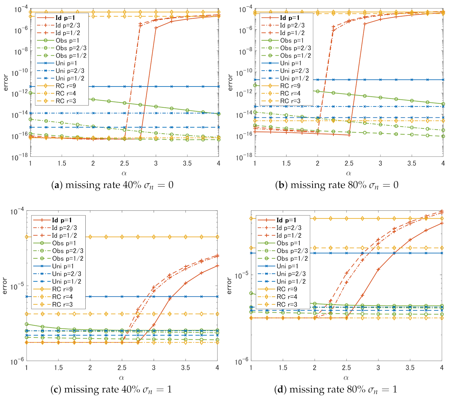
Figure 1. Experimental results for the original tensor with the order 3 and the rank 4. (ad) are the results of varying the missing rate and the standard deviation of the noise σ n during the observation process. The horizontal axis of the graph is the parameter α used for determining the weights and the vertical axis is the error between the estimated tensor and the original tensor calculated by each method. Red, green, and blue indicate the results for the proposed method (Algorithm 1) with different types of weight vectors— w Id , w Obs , and w Uni , respectively—and yellow is the result of the rank-constrained minimization. The line type corresponds to the value of the parameter p or r.
Signals 02 00010 g001
Figure 2. Experimental results for the original tensor with the order 3 and the rank 5. The results of different missing rates and the standard deviations are shown in (ad) and the meaning of the axes and of the colors and types of lines are the same as in Figure 1. Although the rank of the original tensor is different, the relative performance of all methods shows a similar trend in Figure 1. This supports the fact that our conclusions in Section 4.2 are independent of the rank of the original tensor.
Signals 02 00010 g002
Figure 3. Experimental results for the original tensor with the order 4 and the rank 2. The results of different missing rates and the standard deviations are shown in (ad) and the meaning of the axes and of the colors and types of lines are the same as in Figure 1. Although the rank and the order of the original tensor are different, the relative performance of all methods shows a similar trend to Figure 1. This supports the fact that our conclusions in Section 4.2 are independent of the rank and the order of the original tensor.
Signals 02 00010 g003
Figure 4. Experimental results for the original tensor with the order 4 and the rank 3. The results of different missing rates and the standard deviations are shown in (ad) and the meaning of the axes and of the colors and types of lines are the same as in Figure 1. Although the rank and the order of the original tensor are different, the relative performance of all methods shows a similar trend to Figure 1. This supports the fact that our conclusions in Section 4.2 are independent of the rank and the order of the original tensor.
Signals 02 00010 g004
Figure 5. The flowchart for determining a method and parameter for the low-rank tensor recovery problem.
Signals 02 00010 g005
Publisher’s Note: MDPI stays neutral with regard to jurisdictional claims in published maps and institutional affiliations.