Dynamic Model Averaging in Economics and Finance with fDMA: A Package for R

Abstract

The described R package allows to estimate Dynamic Model Averaging (DMA), Dynamic Model Selection (DMS) and Median Probability Model. The original methods, and additionally, some selected modifications of these methods are implemented. For example the user can choose between recursive moment estimation and exponentially moving average for variance updating in the base DMA. Moreover, inclusion probabilities can be computed in a way using “Google Trends” data. The code is written with respect to minimise the computational burden, which is quite an obstacle for DMA algorithm if numerous variables are used. For example, this package allows for parallel computations and implementation of the Occam’s window approach. However, clarity and readability of the code, and possibility for an R-familiar user to make his or her own small modifications in reasonably small time and with low effort are also taken under consideration. Except that, some alternative (benchmark) forecasts can also be quickly performed within this package. Indeed, this package is designed in a way that is hoped to be especially useful for practitioners and researchers in economics and finance.

1. Introduction

This paper is organised as follows. The first section contains the general motivation and information about the package. The next section provides an economic motivation. It is focused on examples from oil market. However, it briefly provides arguments in favour of using model averaging and Bayesian methods in economics. This section contains also short information about the already done researches in which Dynamic Model Averaging (DMA) was used. The third section contains the brief note about the theory of DMA, Dynamic Model Selection (DMS) and Median Probability Model. In the fourth section the main function of this package is described. The fifth section provides some information about the implemented information-theoretic averaging. The sixth section describes some additional functions implemented in fDMA. These functions are mostly some variations about model averaging. The seventh section describes the implementation of the Diebold-Mariano test in such a way that the user can quickly compare forecasts from different models obtained with fDMA. The eighth section describes various minor functions from the package which can be helpful in organizing and making the work faster for a researcher working with fDMA package. The ninth section provides an example of direct application of fDMA for data from oil market. The user greedy for quick familiarizing with the package can directly go to this section and later read the whole paper. He or she can also start from this section and later seek the necessary information in other sections. The final section summarizes the performance of fDMA and compares it with other similar packages.

The very first motivation behind the package described in this paper is to provide an easy and efficient tool for practitioners and/or researchers dealing with DMA. It provides not only the basic implementation of the method originally described by Raftery et al. [1], but also various later modifications of this method, and also some methods more or less linked with DMA. In other words, this package should be able to provide the toolbox for a researcher, which would be large enough to allow for a real-world application of DMA, Dynamic Model Selection (DMS) and Median Probability Model of Barbieri and Berger [2]. Moreover, some subjectively chosen (by the author of the package) alternative methods can also be quickly and easily performed. This should allow the user not only to perform DMA computations, but also to quickly compare the obtained outcomes with some popular alternative methods, in order to be able to compare the obtained results with some other methods. The set of these alternative methods is of course highly subjective. However it is not the most important part of this package, but rather some extra feature which is hoped to make the whole package more useful also for less advanced users.

Although there are already two other competing DMA packages available, i.e., dma and eDMA [3,4], there is still a place for a third one. In particular, the dma is able only to produce the original version of DMA algorithm. It does not allow the user to compute other variations emerging from this algorithm as DMS (Dynamic Model Selection) or Median Probability Model. Moreover, it is explained further in the text, that even the original DMA can be slightly modified, and various researches already proposed some small, but interesting, modification to the original algorithm. The fDMA [5] not only allows to implement these additional features, but even for the unmodified DMA is faster than the dma. In particular, the speed increase in fDMA is gained due to three factors. First, matrix computations are speeded through the use of xts package [6]. Secondly, the crucial part of the code is written with the help of C++ in Rcpp and Rcpp:Armadillo. Thirdly, the user might order the parallel computations [7,8,9,10,11,12].

Actually, in case of speed eDMA is superior over fDMA in the use of both C++ and parallel computations. However, fDMA as little as possible was written in C++, because it is desired that the package can be modified by the user if he or she would find it necessary. Indeed, during the new researches usually some kind of modification of DMA is proposed. Therefore, it is desirable for the package to be rather a flexible tool, than the very efficient, but still a black-box for the user. This is reasonable indeed. From one point of view the applications of DMA are rapidly increasing, meaning that a user-friendly package is necessary. But on the other hand, DMA is still an object of fundamental researches. For instance, Belmonte and Koop [13] considered the usefulness of switching Gaussian state space models in DMA. Hwang [14], Koop [15] and Koop and Korobilis [16] discussed multiple Vector Autoregression (VAR) models in context of DMA. A sort of likelihood tempering and sequential quasi-Bayesian mixture modelling in the presence of models’ misspecification and the data corruption was studied by Reich and Dedecius [17].

Secondly, fDMA still allows the user to use modifications of DMA which eDMA lacks, like for example Occam’s window, Google data, other method of updating variance in the state space equation than the recursive moment estimator, etc. For example, only fDMA is able to compute Median Probability Model out of the discussed packages. Finally, fDMA allows also for information-theoretic averaging (a non-Bayesian method) to be performed similarly like DMA, and some other methods. In this way, the user can not only compute DMA, DMS and Median Probability Model, but also compare the outcomes with some alternative methods. Such a feature is actually important in practical applications. Of course, fDMA is not any try to compete with packages solely devoted to these alternative methods. It is rather an additional feature that helps to do the necessary work in a very quick and simple way in R [18], or the wrapper of the existing R packages allowing to present the outcomes in a consistent way [19,20,21,22,23,24,25]. Also packages graphics, grDevices, parallel, stats, utils are used by fDMA.

Classes and methods are available in fDMA package. In particular, outputs can be easily visualised with print, summary and plot. In case of plots, the user can specify plot(x,non.interactive=TRUE) in order to plot all possible plots for the object x without the menu. If not specified, non.interactive=FALSE is used, i.e., the user through the menu has to choose the type of plot he or she wants. The package is available from CRAN [5]. It can be easily installed:

R> install.packages("fDMA")

The manual for the package contains numerous examples and the most basic literature references are provided there.

Finally, it should be mentioned that there exist packages implementing the ”static” Bayesian Model Averaging (BMA) and Bayesian Model Selection (BMS). They are BMA for BMA [26], BMS [27] for BMS and mlogitBMA [28] for BMA with multinomial logit data. Moreover, as BMA is a quite popular method in social and nature sciences, there exist also packages which apply BMA/BMS as a part of certain modelling schemes. In particular, ensembleBMA [29] uses BMA to create probabilistic forecasts from ensemble forecasts and weather observations. metaBMA [30] uses BMA for some meta-analysis models. INLABMA [31] fits spatial econometrics models with the help of BMA. dga [32] uses BMA for capture-recapture. spatial.gev.bma [33] allows to fit a hierarchical spatial model for the generalized extreme value distribution with the option of Bayesian Model Averaging over the space of covariates. MHTrajectoryR [34] uses BMS in logistic regression for the detection of adverse drug reactions.

2. Economic Motivation

Now, the economic motivation for the use of the implemented methods is provided. Indeed, DMA joins a few features of econometric modelling together. First of all, the final forecast is produced out of several regression models by model averaging. Secondly, the method is a Bayesian one, i.e., probabilities are interpreted in a degree-of-belief way. Indeed, for example the DMA forecast for time t is made on the basis of data up to time $t-1$ only. Moreover, the gain of a new data results in a direct parameters’ updating. Therefore, in DMA both regression coefficients and weights ascribed to the models vary in time.

Bayesian methods are not the mainstream of modern econometrics. However, these methods are gaining more and more interest recently. There are various reason for this. First of all, one can link this to the increasing amount of data that a potential researcher has to cope with in his or her research. Due to the technological progress usually one is faced with the case of many potential explanatory variables. Despite the fact that most of them are probably unimportant, the researcher usually does not know which ones should be rejected.

Of course, up to some point conventional methods can still be used. But unfortunately precise estimates of parameters usually cannot be done due to the lack of enough information. The simplest example is when the number of explanatory variables is greater than the number of observations in the time-series. For example, even in the case of a linear regression the standard ordinary least squares estimation a singular matrix would emerge, resulting in the impossibility of taking its inverse. In the Bayesian framework, still a meaningful formula is derived. It also seems that the Bayesian methods deal better with over-parametrization and over-fitting issues. Some kind of conventional methods to deal with omitted variables bias, like hypothesis testing to select the ”true” model out of many possible is also problematic in case of many variables due to computational issues [35]. All this results in an increasing concern about the Bayesian methods in new researches, which is thoroughly described in various reviews and monographs [36,37,38,39,40,41].

In this place it is worth to mention that various approaches can be found in recent trends in forecasting. Narrowing, as an example, to oil price, forecasting methods can usually be classified into time-series models, structural models and some other methods like machine learning, neural networks, etc. This is well described in the recent extensive surveys [42,43,44,45,46]. Generally, time-series models are focused on modelling rather volatility than the spot prices. Structural models by definition include causal relations, but they usually have a good predictive power in certain periods and very poor in others. Also, the other methods, basing on wavelet decomposition, neural networks, etc. usually omit influence of other factor and focus on a single time-series [47,48,49,50,51,52,53,54,55,56,57,58,59,60,61]. These makes DMA an interesting method for a practitioner.

The next aspect of DMA is that it allows for regression coefficients to be time-varying. Indeed, in the presence of both slow and rapid (structural breaks) changes in economy, such a property of the econometric model is very desirable. Of course, such an approach also exists in conventional methodology, for example, as recursive or rolling window regressions. But since the seminal paper by Kalman [62] more sophisticated methods are usually used. They allow to incorporate uncertainty of variables’ estimates in the presence of noise in the measurement, etc. As a result more accurate estimates are obtained [63].

Another important feature of DMA is that the final forecast comes from forecast combination. As already mentioned in many economic problems the researcher is not sure which variables should be included in the model. In other words, narrowing for instance to linear regression models, the research has to cope with uncertainty about the model. Of course, one approach is to use some methods to uncover the ”true” model out of all considered. Actually, one of the assumptions of DMA is that such a ”true” model exists, so with upcoming new data its weight should increase. But the forecast in DMA is formulated as a weighted average from the predictions of all possible models concerned. In this way DMA incorporates a model averaging technique. Since the seminal paper by Bates and Granger [64] it is know that forecast combination can be beneficial. Bates and Granger [64] provided an example when forecast combination with suitable setting the weights for two models can result in smaller Mean Square Error than those of two separate models. Yet, since then in many cases it was found that not only on a theoretical ground model averaging can be beneficial over model selection. Just in case of practical applications, i.e., seeking a method to produce smaller errors, to better fit the historical data, and/or to produce more accurate forecast, it was found that model averaging can be useful for practitioners [65,66,67,68,69,70,71]. Indeed, model averaging is a popular technique not only in the Bayesian setting. Various approach are developed, basing on different underlying theories [2,72,73,74,75,76,77,78,79,80]. Recently, a very detailed surveys in model averaging in economics has been written [81,82,83], to which the interested reader is referred.

In economics, model averaging within the Bayesian framework was well adapted in studying the economic growth [84]. However, the examples for fDMA in this paper are taken from the oil market, i.e., the spot oil price is examined. Indeed, this topic was studied, for example, by Drachal [85] and Naser [86]. Therefore, the reader interested in financial and economical perspective is referred to these papers. Herein, just fDMA package is described, and oil market data serve just as an illustrative examples how to use the package – not how to do a good economic research. In particular, the data set is greatly reduced in order to execute the examples in a few seconds.

Therefore, in 

Table 1. Possible drivers of spot oil price.

Driver	Reason to Treat as a Potential Driver and Source
Interest rate	Higher rate results in higher price of a non-renewable resource (Hotelling’s rule). Higher rate results in lower price of a commodity because of the cost of holding inventory [87].
Supply and demand	Increase in demand results in price increase. Increase in supply – in price decrease. This is sometimes known as the law of supply and demand [88,89,90,91,92,93,94].
Exchange rates	The price of oil in the domestic currency changes as the exchange rate changes. This has different implications for oil-exporting and oil-importing countries [95,96,97,98,99,100,101,102].
Stock markets	Empirically it was found that oil price and stock indices are usually following similar time paths. Also, that predictive accuracy of oil price forecasts increase when data from stock markets is used. Oil price can affect interest rates, production, GDP, which further affects the expected free cash flow. This further affects stock prices. Moreover, there is a rising financialization of oil market, i.e., since 2000s increasing links between oil and stocks markets [95,103,104,105,106,107,108,109110111112].
Speculative forces	Links between spot and futures markets. Above mentioned financialization. Trading on OTC electronic exchanges [113,114,115,116,117,118].
Inventories	They can be released to cover supply shortages, as so called buffer inventory. Also, they can be stored to be sold at higher prices in the future. This is called speculative inventory [119,120,121,122].
Oil price volatility	It has a direct effect on the energy sector. Higher volatility might put pressure on consumers to switch to alternative energy sources, and therefore, demand decrease [123,124].
Other commodities	Empirically, correlations between oil price and prices of other commodities, for example gold, are found. Gold price usually increase during market downturns [96,125,126,127,128,129,130,131,132].
Economic activity	Economic growth stimulates oil demand [109,133,134,135,136,137,138,139,140].
Policy uncertainty	Empirically, economic policy uncertainty increases predictive accuracy of oil price forecasts. Usually, positive uncertainty shocks affect commodity prices returns negatively [141,142,143].

a collection of several potential oil price drivers is presented. These relationships, their strengths and direction are also found to be time-varying. It has to be stressed that variables in this table are only potential oil price drivers. Although in some cases direct causal relationship can be found from literature, it is enough just to have a tentative supposition that given variable might be somehow linked with oil price. In this way the list of potential drivers is reasonable, but still uncertainty about them exists.

As mentioned, for the most detailed economic analysis of the literature the reader is referred to the already mentioned papers. Moreover, it is worth to notice that there exist a few, both up-to-date and extensive, reviews of various forecasting techniques of oil price [42,43,44,45,46]. Also, it is interesting to consider how the Bayesian approach in general is used in forecasting oil price. Basing on the Scopus database and narrowing to last 10 year, it can be concluded that conventional methods or those based on, for example, neural networks and machine learning are still more popular. But interestingly, the number of papers with the Bayesian approach has been rapidly increasing over the past few years [85,86,96,99,115,135,137,143,144,145,146,147].

Some modification of DMA implemented in fDMA allows to include data about Internet queries. Indeed, use of such data in forecasting is raising popularity. It was also found useful in modelling oil market [148]. The exact use in DMA is described later in this paper.

Finally, it is worth to notice that DMA was already applied to several markets. Except the already mentioned oil market, this method was used in forecasting gold price [149,150,151], cooper price [152], carbon market [153], inflation [154,155,156,157,158,159], GDP [158,159], real estate markets [160,161,162], exchange rates [163,164] and stock markets [151,165,166,167,168]. It is also clear that this method has gained an increasing interest in economics since 2015.

3. Theoretical Framework

In this section the theoretical framework of fDMA is shortly described. In particular, Dynamic Model Averaging (DMA), Dynamic Model Selection (DMS), Median Probability Model and information- theoretic averaging.

3.1. Dynamic Model Averaging (DMA)

DMA was introduced in great details in the original paper by [1]. However, below a short exposition is presented, necessary to understand what each function in fDMA does.

Suppose that $y_t$ is the forecast time-series (dependent variable), and let $x_t^{(k)}$ be the column vector of independent variables in k-th regression model. For instance, 10 potential oil price drivers are listed in Table 1. If each of them would be represented by a suitable time-series, then $2^{10}$ possible linear regression models can be constructed. Indeed, each variable can be included or not included in a model. So, 2 choices are possible for each variable, constituting $2^{10}$ possibilities. This includes a model with constant only. So, in general having potentially useful m independent variables, up to $K=2^m$ models can be constructed. In other words the state space model is given by

$$y_t={(x_t^{(k)})}^{\top }{\theta }_t^{(k)}+{ϵ}_t^{(k)},$$

(1)

$${\theta }_t^{(k)}={\theta }_{t-1}^{(k)}+{\delta }_t^{(k)},$$

where $k=1,\cdots ,K$ and ${\theta }_t$ is the column vector of regression coefficients. It is assumed that errors follow the normal distribution, i.e., ${ϵ}_t^{(k)}\sim \mathcal{N}(0,V_t^{(k)})$ and ${\delta }_t^{(k)}\sim \mathcal{N}(0,W_t^{(k)})$.

Please notice herein that having m potential explanatory variables $2^m$ is the upper limit of constructed models. However, all methodology described in this paper (if not stated otherwise) is applicable for any subset of these $2^m$ models, i.e., $K\le 2^m$.

Let $L_t=k$ if the process is governed by k-th model in time t. The evolution can be determined by $K\times K$ transition matrix $(p_{k,l})$ with $p_{k,l}=p[L_t=l|L_{t-1}=k]$. For large K computations are impossible, therefore an approximation is necessary. In particular, let ${\theta }_t={({\theta }_t^{(1)},\cdots ,{\theta }_t^{(K)})}^{\top }$, then the underlying state consists of the pair $({\theta }_t,L_t)$. Its probability distribution is $p({\theta }_t,L_t)={\sum }_{k=1}^K[p({\theta }_t^{(k)}|L_t=k)p(L_t=k)]$. Suppose that the conditional distribution of the state in time $t-1$ knowing the data up to time $t-1$, i.e., $Y^{t-1}=\{y_1,\cdots ,y_{t-1}\}$, is known from $p({\theta }_{t-1},L_{t-1}|Y^{t-1})={\sum }_{k=1}^K[p({\theta }_{t-1}^{(k)}|L_{t-1}=k,Y^{t-1})p(L_{t-1}=k|Y^{t-1})]$, where the conditional distribution of ${\theta }_{t-1}^{(k)}$ is approximated by ${\theta }_{t-1}^{(k)}|L_{t-1}=k,Y^{t-1}\sim N({\widehat{\theta }}_{t-1}^{(k)},E_{t-1}^{(k)})$. Two steps are used in the approximation. First, $L_t$ is predicted. Next, ${\theta }_t^{(k)}|L_t$ is predicted.

Let ${\pi }_{t-1|t-1,k}=p[L_{t-1}=l|Y^{t-1}]$. Then ${\pi }_{t|t-1,k}={\sum }_{l=1}^K{\pi }_{t-1|t-1,l}{p}_{k,l}$, where ${\pi }_{t|t-1,k}=p[L_t=k|Y^{t-1}]$. However, the approximation can be used, i.e.,

$${\pi }_{t|t-1,k}\approx \frac{{({\pi }_{t-1|t-1,k})}^{\alpha }}{{\sum }_{l=1}^K{({\pi }_{t-1|t-1,l})}^{\alpha }}$$

(2)

where $\alpha$ is a forgetting factor, i.e., a fixed number between 0 and 1. Further, ${\pi }_{t|t-1,k}$ are called posterior probabilities.

During the numerical approximations, zeros can emerge in Equation (2). Therefore, following [1], in the package Equation (2) is replaced by

$${\pi }_{t|t-1,k}=\frac{{({\pi }_{t-1|t-1,k})}^{\alpha }+c}{{\sum }_{l=1}^K\left({({\pi }_{t-1|t-1,l})}^{\alpha }+c\right)},$$

(3)

where $c=0.001·2^m$.

Next, ${\theta }_t^{(k)}|L_t=k,Y^{t-1}\sim \mathcal{N}({\widehat{\theta }}_{t-1}^{(k)},E_{t-1}^{(k)}+W_t^{(k)})$, where

$$E_{t-1}^{(k)}+W_t^{(k)}\approx E_{t-1}^{(k)}·{\lambda }^{-1},$$

(4)

where $\lambda$ is the next forgetting factor between 0 and 1.

Additionally, ${\pi }_{t|t,k}=p[L_t=l|Y^t]$ can be computed in the following way

$${\pi }_{t|t,k}=\frac{{\pi }_{t|t-1,k}{f}_k(y_t|Y^{t-1})}{{\sum }_{l=1}^K{\pi }_{t|t-1,l}{f}_l(y_t|Y^{t-1})},$$

(5)

where $f_k(y_t|Y^{t-1})$ is the predictive density of k-th model at $y_t$. But this is given as the density of

$$\mathcal{N}({(x_t^{(k)})}^{\top }{\widehat{\theta }}_{t-1}^{(k)},V_t^{(k)}+{(x_t^{(k)})}^{\top }{E}_{t-1}^{(k)}{\lambda }^{-1}{x}_t^{(k)}).$$

(6)

Variance $V_t^{(k)}$ is updated by the recursive moment estimation, i.e.,

$$V_t^{(k)}={(1-t)}^{-1}{\widehat{V}}_{t-1}^{(k)}+t^{-1}[{(e_t^{(k)})}^2-{(x_t^{(k)})}^{\top }{E}_{t-1}^{(k)}{\lambda }^{-1}{x}_t^{(k)}],$$

(7)

where

$$e_t^{(k)}=y_t-{(x_t^{(k)})}^{\top }{\widehat{\theta }}_{t-1}^{(k)}$$

(8)

is the error term from the one-ahead prediction of k-th model. If the updated $V_t^{(k)}\le 0$, then it is taken $V_t^{(k)}={\widehat{V}}_{t-1}^{(k)}$. Moreover, with respect to ${\theta }_t^{(k)}|L_t=k$ and $Y^t\sim \mathcal{N}({\widehat{\theta }}_t^{(k)},E_t^{(k)})$ regression coefficients are updated in the following way

$${\widehat{\theta }}_t^{(k)}={\widehat{\theta }}_{t-1}^{(k)}+E_{t-1}^{(k)}{\lambda }^{-1}{x}_t^{(k)}{(V_t^{(k)}+{(x_t^{(k)})}^{\top }{E}_{t-1}^{(k)}{\lambda }^{-1}{x}_t^{(k)})}^{-1}{e}_t^{(k)}.$$

(9)

On the other hand, $E_t^{(k)}$ is updated in the following way

$$E_t^{(k)}=E_{t-1}^{(k)}{\lambda }^{-1}-E_{t-1}^{(k)}{\lambda }^{-1}{x}_t^{(k)}{(V_t^{(k)}+{(x_t^{(k)})}^{\top }{E}_{t-1}^{(k)}{\lambda }^{-1}{x}_t^{(k)})}^{-1}{(x_t^{(k)})}^{\top }{E}_{t-1}^{(k)}{\lambda }^{-1}.$$

(10)

In order to set the above recursive computations some initial values have to be set. Assuming that initially all K models are equally probable (i.e., setting the non-informative prior) the below formula is given

$${\pi }_{0|0,k}=\frac{1}{K}$$

(11)

for every $k=1,\cdots ,K$, and the vectors of regression coefficients are initially set to zeros, i.e.,

$${\theta }_0^{(k)}=0.$$

(12)

Moreover,

$$E_0^{(k)}=\left[\begin{array}{cccc}{\beta }^2+\mathrm{Var}(y)& 0& \cdots & 0\\ 0& \frac{\mathrm{Var}(y)}{\mathrm{Var}(x_1^{(k)})}& \cdots & 0\\ ⋮& ⋮& \ddots & 0\\ 0& \cdots & \cdots & \frac{\mathrm{Var}(y)}{\mathrm{Var}(x_{j_k}^{(k)})}\end{array}\right],$$

(13)

where $j_k$ is the number of dependent variables in k-th model and $\beta$ is the estimated intercept term in a linear regression model with y as the dependent variable and whole x as the independent variables.

It can happen during the numerical estimations that some $\mathrm{Var}(x_i^{(k)})$ will be approximated to 0. In such a case, in fDMA if zero value emerge, then it is replaced by a small constant computed analogously as in Equation (3).

Finally, the DMA forecast is given by

$${\widehat{y}}^{\mathrm{DMA}}=\sum _{k=1}^K{\pi }_{t|t-1,k}{\widehat{y}}_t^{(k)}=\sum _{k=1}^K{\pi }_{t|t-1,k}{(x_t^{(k)})}^{\top }{\widehat{\theta }}_{t-1}^{(k)}.$$

(14)

All in all, the above scheme can be viewed as estimating K time-varying parameters regression models (TVP), and then averaging them with a set of recursively updated weights. In particular, having the variables $y_t$ and $x_t^{(k)}$ the user has to specify the forgetting parameters $\alpha$ and $\lambda$, and the initial variances $V_0^{(k)}$. Then, the other initial parameters are set through Equations (11)–(13). Next, the process is updated recursively. Each of K models are estimated through Equations (1), (8), (10), (6), (9) and (7). Weights are updated by Equations (2) and (5).

It is worth to notice that if $\alpha =1$ and $\lambda =1$ is taken, then the above scheme reproduces in a recursive way Bayesian Model Averaging (BMA).

3.2. Dynamic Model Selection (DMS)

Dynamic Model Selection (DMS) is based on the same idea, as the one behind DMA. The only difference is that in DMA model averaging is performed, whereas in DMS – model selection. In other words, for each period t the model with the highest posterior probability is selected. This means that just Equation (14) is modified to

$${\widehat{y}}^{\mathrm{DMS}}={\widehat{y}}_t^{(h_t)},$$

where $h_t$ denotes this model out of K models, which corresponds to the highest ${\pi }_{t|t-1,k}$ given by Equation (2).

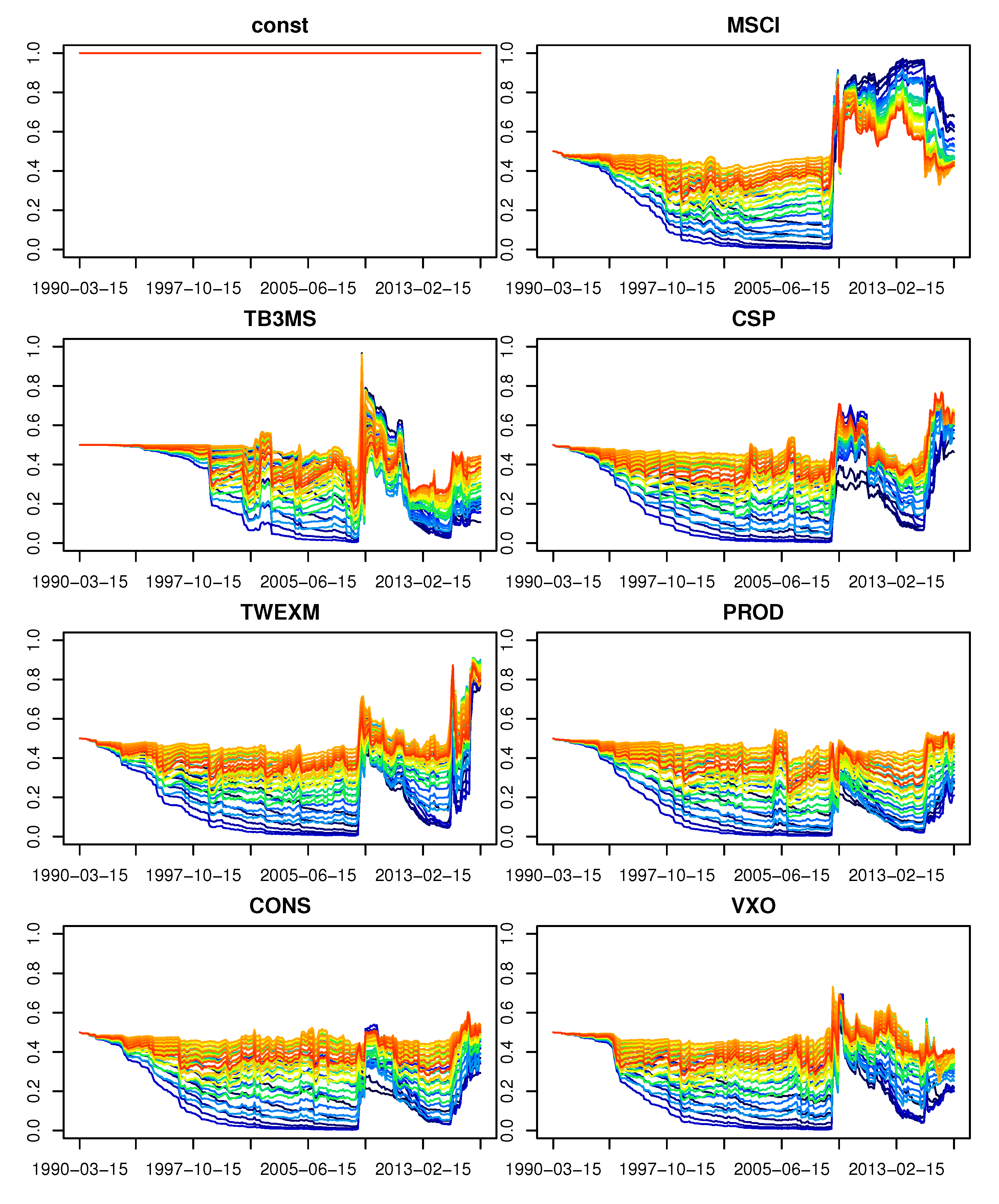
3.3. Relative Variable Importance

Before proceeding further it is necessary to explain the concept of a relative variable importance.

The idea is just to sum posterior probabilities of models, which contain given explanatory variable. In other words, consider the posterior probabilities given by Equation (2), but not for all $k=1,\cdots ,K$ – only for those models, which contain the given variable as explanatory one:

$$\mathrm{RVI}{(x_j)}_t=\sum _{k=1}^K{\pi }_{t|t-1,k}{\mathbb{1}}_k(x_j),$$

(15)

where ${\mathbb{1}}_k(x_j)=1$ if k-th model contains $x_j$ as an explanatory variable, and ${\mathbb{1}}_k(x_j)=0$ otherwise.

Of course, this concept can be applied both in case of model averaging and model selection. Simply, in model selection in Equation (15) will be no summing, but just one term – the one corresponding to the selected model. So in such a case relative variable importance reduces to trivial outcome. Generally, this concept can be easily transferred to other model averaging schemes, like the information-theoretic one, for instance. The idea is just to replace the posterior probabilities ${\pi }_{t|t-1,k}$ by suitable weights. Indeed, ${\pi }_{t|t-1,k}$ are just weights ascribed to the averaged models in DMA.

Actually, this concept is very interesting from the economical point of view. Indeed, in the mentioned applied papers which uses DMA methodology, this concept has been used and discussed. However, a great caution has to be taken. First of all, the term importance is used, in order not to misuse with statistical significance. Indeed, relative variable importance is not connected with any statistical test, it is also a very relative measure. It measures how the given variable becomes more “appreciated” within the set of considered models.

Secondly, it is not known how to deal with the situation that quite high weight is ascribed to the model containing given variable and some other variables. In other words, it might happen that such a model is preferred not because of including the variable the researcher is interested in, but because of the joint “importance” of this variable and the other ones in the model. The topic of jointness in Bayesian framework is a separate research problem [169].

Another, directly coming to the mind idea is to consider the expected number of variables. In other words, to consider the weighted average of the number of explanatory variables (including constant term if present), where the weights are given by posterior probabilities (or other suitable weight, if other kind of model averaging is performed). In other words, to consider

$${\mathrm{EV}}_t=\sum _{k=1}^K\left({\pi }_{t|t-1,k}\sum _{j=0}^m{\mathbb{1}}_k(x_j)\right),$$

(16)

where $x_0$ stands for the constant term.

3.4. Median Probability Model

Barbieri and Berger [2] observed that selecting the model with highest posterior probability, although somehow desirable under very general conditions, is still optimal only in case of competing only two models, and also in the case of linear models having orthogonal design matrices. But not in general conditions. Therefore, they proposed Median Probability Model.

In the already presented framework the application of their approach is very similar to DMS. However, the selected model is the one which contains as explanatory variables exactly those whose relative variable importance is equal to or greater than $0.5$.

It should be noticed that if $K=2^m$, i.e., all possible models are considered such a model always exist. However, if $K<2^m$ it might not exist.

3.5. Internet Searches

Koop and Onorante [170] proposed to modify Equation (2) in such a way that it includes the information from Internet queries. The motivation behind this is that the weight ascribed to the model should include the information about the interest of investors in variables in this model. For instance, if there is an increasing interest in exchange rates, then models with this explanatory variable should be given somehow higher weights than the models without this variable. The data about Internet searches are available directly from, for example, Google [171]. These data are the numbers between 0 and 100. Moreover, they correspond not to the absolute volume of searches, but to the relative one – in comparison to all searches. Therefore, these numbers can reasonable represent interest in given variable (representing some economic factor). In order, to interpret these data as probabilities they just have to be divided by 100 to fit between 0 and 1. They are called Google probabilities in this paper.

Of course, it is another topic how to suitably choose search terms in the context of a particular research study. Moreover, how to include this information in model averaging is also an open topic. What Koop and Onorante [170] proposed is, first, to compute

$$p_{t,k}=\prod _{i\in IN}{g}_{i,t}·\prod _{j\in OUT}(1-g_{j,t}),$$

(17)

where $g_{i,t}$ denotes the Google probability of i-th variable at time t, i.e., the number obtained from Google Trends [171] corresponding to Internet searches of the query associated with i-th variable, divided by 100; and $IN$ denotes variables included in k-th model, and $OUT$ denotes variables not included in k-th model.

It can happen during the numerical estimations that some ${\prod }_{i\in IN}{g}_{i,t}$ or ${\prod }_{j\in OUT}(1-g_{j,t})$ will be approximated to 0. In such a case, in functions in fDMA it will be replaced by a small constant computed analogously as in Equation (3).

Next, Equation (2) is replaced with

$${\pi }_{t|t-1,k}=\omega ·\frac{{({\pi }_{t-1|t-1,k})}^{\alpha }}{{\sum }_{l=1}^K{({\pi }_{t-1|t-1,l})}^{\alpha }}+(1-\omega )·p_{t,k},$$

(18)

where $\omega$ is a fixed parameter, i.e., a number between 0 and 1. Of course, in case of $\omega =1$ this modification replicates the basic DMA without Google data.

Naturally, for any other kind of model averaging the above concept can be similarly mimicked. The only thing is to replace the weights used in that forecast combination scheme, $w_{t,k}$, by $\omega ·w_{t,k}+(1-\omega )·p_{t,k}$.

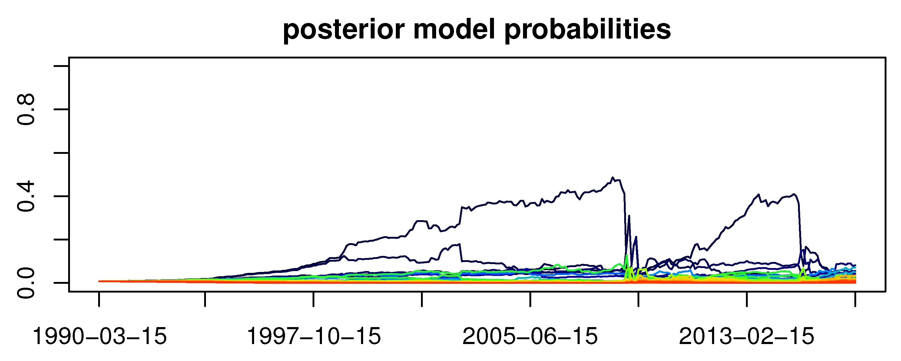
3.6. Dynamic Occam’s Window

Actually, DMA is quite computationally demanding technique. Generally, every new extra explanatory variable added to DMA increases the time of computations twice. Therefore, if dealing with around 10 potential explanatory variables DMA still can be performed on an average computer machine. However, if the number of variables grows and is around 20 the time needed grows in exponential pattern. The use of simply faster machines, or more machines in parallel way is still not a satisfactory solution.

Onorante and Raftery [172] proposed to apply dynamic Occam’s window. In particular, their procedure, modifying DMA, can be described in the following steps. It should be noticed that the implementation slightly differs from the one described by Onorante and Raftery [172], but the idea remains unaffected.

Suppose that one would like to estimate DMA for some set of models $\mathcal{M}$ with observations covering the period up to time T. And that this is computationally infeasible, i.e., $\mathcal{M}$ is too large.

The procedure is recursive, in the following sense.

• Assume that the standard DMA was performed for some subset of models ${\mathcal{M}}_t\subset \mathcal{M}$, but for the observations up to time $t\le T$.
• The DMA forecast is produced. It is called DMA-E. Basing on the weights given by Equation (5) the cut-off is performed, i.e., DMA forecast for the period t is made only from models with

  $${\pi }_{t|t,i}\ge C·\underset{k\in {\mathcal{M}}_t}{max}\{{\pi }_{t|t,k}\}.$$

  (19)
  Of course, the weights for the remaining models are normalized to sum up to 1. This forecast is called DMA-R.
• The above cut-off reduces the set of models ${\mathcal{M}}_t$. Such a reduced set is now expanded by new models constructed by adding or removing exactly one explanatory variable from all possible variables to each model in this reduced set of models. The constant term is not included in this adding/removing procedure. As a result, the set of models ${\mathcal{M}}_{t+1}$ is created.
• If $t<T$ Step 1 is performed with the updated set of models. Otherwise, the procedure is stopped.

In order to begin, the initial set of models should be specified, i.e., ${\mathcal{M}}_0$. As ${\mathcal{M}}_0=\mathcal{M}$ is usually too large even for the first step, there are two natural candidates. One can start with some random subset ${\mathcal{M}}_0\subset \mathcal{M}$. The second option is to specify ${\mathcal{M}}_0$ as the models consisting of exactly one explanatory variable. Moreover, the cut-off threshold C between 0 and 1 has to be specified. Moreover, the user should decide which forecast would be of his or her interest: DMA-R or DMA-E.

Of course, the above scheme requires to estimate standard DMA T times, if the length of time-series is T. But the idea behind the above concept is that in certain cases the suitable selection of threshold C can greatly reduce the number of models used in averaging. Therefore, leading to overall speed increase.

Actually, the original version, described by Onorante and Raftery [172] was not making cut-off immediately as in the above presentation. It was allowed for the full initial set $\mathcal{M}$ to be estimated with standard DMA for some short period. However, in majority of tests performed by the author of fDMA such calculations were still taking too much time. Therefore, the idea was kept, but small details are modified in fDMA. Indeed, Onorante and Raftery [172] also stated directly that, for example, the models expansion through adding/removing one explanatory variable might be replaced by some other procedure.

4. Fundamental Functions

In this section the main functions of fDMA are described.

The main function in this package is fDMA. It should be used in the following way.

fDMA(y, x, alpha, lambda, initvar, W = NULL, initial.period = NULL,

  V.meth = NULL, kappa = NULL, gprob = NULL, omega = NULL, model = NULL,

  parallel = NULL, m.prior = NULL, mods.incl = NULL, DOW = NULL,

  DOW.nmods = NULL, DOW.type = NULL, DOW.limit.nmods = NULL,

  progress.info = NULL, forced.models = NULL,

  forbidden.models = NULL, forced.variables = NULL,

  bm = NULL, small.c = NULL, fcores = NULL, mods.check = NULL,

  red.size = NULL, av = NULL)

Below the arguments for this function are explained:

• y should be a numeric or a column matrix representing the dependent variable. If it is xts, then plots will have time index on the x axis,
• x should be a matrix of explanatory variables. Observations should go by rows, and different columns should correspond to different variables,
• alpha should be a numeric representing the forgetting factor $\alpha$ used in Equation (2),
• lambda should be a numeric representing the forgetting factor $\lambda$ used in Equation (4), It is also possible to specify lambda as numeric vector. Then, its values are automatically ordered in descending order, and if numbers are not unique they are reduced to become unique. The idea is that if more than one value is given for lambda, then the model state space, i.e., mods.incl, is expanded by considering all these models with given values of lambda. The outcomes of fDMA are then ordered by columns in a way that first outcomes from models with first value of lambda are presented, then from models with second value of lambda, etc. This specification can be used if the user would like to perform the model combination scheme in which models specified by mods.incl are additionally treated as separate new models each with different value of $\lambda$ given by lambda. Such an approach is given by Raftery et al. [1] at the end of their paper,
• initvar should be a numeric. It represents the initial variances in the state space equation, $V_0^{(k)}$. It is taken the same for all $k=1,\cdots ,K$ models,
• W is optional. If W = “reg” then $E_0^{(k)}$ are specified in the initial step as in Equation (13). On the other hand, if a positive numeric is given, then Equation (13) is modified in the following way:

  $$E_0^{(k)}=\left[\begin{array}{cccc}W& 0& \cdots & 0\\ 0& W& \cdots & 0\\ ⋮& ⋮& \ddots & 0\\ 0& \cdots & \cdots & W\end{array}\right].$$
  By default W = “reg”,
• initial.period is optional. This numeric indicates since which moment MSE (Mean Squared Error) and MAE (Mean Absolute Error) should be computed. As fDMA already produces some forecast quality measures, the user might require to treat some first observations as “training period”. By default the whole sample is used to produce forecast quality measures, i.e., initial.period = 1,
• V.meth is optional. If V.meth = “rec”, then the recursive moment estimator as in Equation (7) is used. If V.meth = “ewma”, then the exponentially weighted moving average (EWMA) is used, i.e., Equation (7) is replaced by

  $$V_t^{(k)}=\kappa ·{\widehat{V}}_{t-1}^{(k)}+(1-\kappa )·{(e_t^{(k)})}^2,$$

  (20)

  where $\kappa$ (kappa) has to be also specified. EWMA is a common estimator in finance. For instance, Riskmetrics calls $\kappa$ a decay factor and suggests $\kappa =0.97$ for monthly data, and $\kappa =0.94$ for daily data. Koop and Korobilis [157] used $\kappa =0.98$ for quarterly data. EWMA was also used by them when ARCH effects in Equation (1) were suspected, as other methods would increase the computational burden too much. By default V.meth = “rec” is used,
• kappa is optional numeric. It has to be specified if V.meth = “ewma”. Then, it corresponds to $\kappa$ in Equation (20),
• gprob is optional. This matrix represents Google probabilities, $g_{i,t}$, as in (17). In other words, columns should correspond to different explanatory variables, i.e., the columns of x. These values should be not a direct Google Trends data, but these search volumes index divided by 100. It should also be noticed that gprob is not lagged one period back automatically inside the function. If nrow(gprob) < length(y), then the method by Koop and Onorante [170] is used for the last nrow(gprob) observations. For the preceding ones the original method by Raftery et al. [1] is used. In such case a warning is generated.
• omega is optional. This numeric has to be specified if gprob is used, and it represents the parameter $\omega$ from Equation (18),
• model is optional. If model = “dma” then Dynamic Model Averaging (DMA) is computed. If model = “dms” then Dynamic Model Selection (DMS) is computed. If model = “med” then Median Probability Model is computed. By default model = “dma” is used,
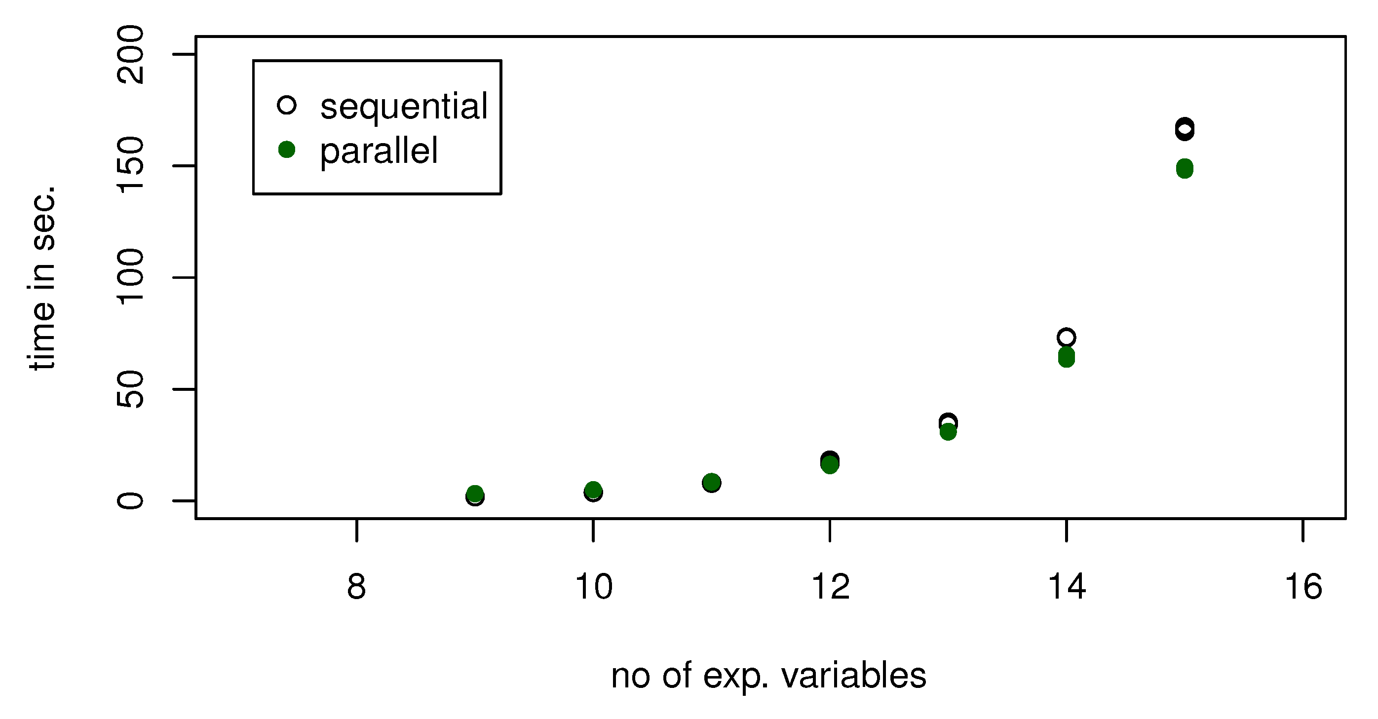
• parallel is optional. This logical indicates whether parallel computations should be used. If parallel = TRUE all cores less 1 are used. (But it can be changed, see fcores below.) However, it should be noticed that parallel computations are not always desired. It can happen that additional time for overheads will take too much time, and sequential computations would be faster. Therefore, if dynamic Occam’s window is applied, and parallel = TRUE, then parallel computations are turned on only for rounds in which $2^{10}$ or more models are estimated. This was chosen basing on some tests. The reason for such a methodology is that forcing all rounds to be computed in a parallel way can result in a situation that in rounds where too few models are generated overheads would increase the computation time. By default parallel = FALSE is used,
• m.prior is optional. This numeric represents a parameter $\pi$ for general model prior. In other words, Equation (11) can be replaced by

  $${\pi }_{0|0,k}={\pi }^{p_k}·{(1-\pi )}^{m-p_k},$$

  (21)

  where $p_k$ is the number of variables including constant term in k-th model and m is the total number of potential explanatory variables including constant considered in the forecast combination scheme [173,174]. By default m.prior = 0.5, which corresponds to the uniform distribution, i.e., non-informative priors. Then, Equation (21) reduces to Equation (11). The interpretation of $\pi$ is that the prior expected number of explanatory variables in the model is $m·\pi$, so by changing $\pi$ the user can modify the initial weights giving more attention to models with more variables or to rather parsimonious models,
• mods.incl is optional. This matrix indicates which models should be used for the estimation. The first column indicates inclusion of a constant. In other words, different models are differentiated by rows, whether columns correspond to the explanatory variables. Inclusion of a variable is indicated by 1, omitting by 0. By default all possible models with a constant are used,
• DOW is optional. This numeric represents the threshold for dynamic Occam’s window, i.e., the parameter C in Equation (19). If DOW = 0, then no dynamic Occam’s window is applied. By default DOW = 0 is used. Dynamic Occam’s window can be applied only to Dynamic Model Averaging (DMA), i.e., if model = “dma”,
• DOW.nmods is optional. This numeric indicates the initial number of models for dynamic Occam’s window. Of course, it should be less than the number of all possible models and larger than or equal to 2. These models are randomly chosen. So if the user wants to start with all models specified by mods.incl, then he or she should just specify DOW.nmods equal to the number of all models given by mods.incl. If DOW.nmods = 0, then initially models with exactly one explanatory variable and a constant term are taken. By default DOW.nmods = 0 is used,
• DOW.type is optional. DOW.type = “r” corresponds to DMA-R in dynamic Occam’s window. DOW.type = “e” corresponds to DMA-E in dynamic Occam’s window. By default DOW.type = “r” is used,
• DOW.limit.nmods is optional. This numeric indicates the maximum number of models selected by dynamic Occam’s window. In other words, it can happen that the cut-off specified by C in dynamic Occam’s window will leave too many models for efficient computations. If the user wants to use the additional limitation, i.e., to be sure that no more than DOW.limit.nmods models are left after the cut-off, this parameter should be specified. By default no limit is set,
• progress.info is optional. This logical is applicable only if dynamic Occam’s window is used. Otherwise it is ignored. If progress.info = TRUE then the number of the current recursive DMA computation round and number of models selected for this round are printed on the screen as the computations go. This feature can be useful if the user is uncertain about the existence of some bottleneck in dynamic Occam’s window. For instance, the cut-off level can result in reasonably small number of model up to some period, but then suddenly too many models would be taken. Therefore, this feature helps the user to have a preview on what is going on with dynamic Occam’s window in real time. By default progress.info = FALSE,
• forced.models is optional. This matrix is applicable only if Dynamic Occam’s Window is used. Otherwise it is ignored. It indicates models that have to be always included in the expanded set of models. The use is similar as that of models.incl. By default forced.models = NULL,
• forbidden.models is optional. This matrix is applicable only if Dynamic Occam’s Window is used. Otherwise it is ignored. It indicates models that cannot be present in the expanded set of models. The use is similar as that of mods.incl. By default forbidden.models = NULL,
• forced.variables is optional. This vector is applicable only if Dynamic Occam’s Window is used. Otherwise it is ignored. It indicates variables that have to be always included in models constituting the set of expanded models. The use is similar as that of mods.incl. The first slot indicates the inclusion of constant. By default forced.variables = NULL,
• bm is optional. This logical indicates whether Auto ARIMA benchmark forecast should be computed. In particular, these benchmarks are naive forecast (i.e., all forecasts are set to be the value of the last observation), which is always computed. But Auto ARIMA (auto.arima from forecast) by Hyndman and Khandakar [20] is optional. By default bm = FALSE,
• small.c is optional. Specifying this numeric allows to modify the value of c in Equation (3),
• fcores is optional. Specifying this numeric allows to control the number of cores that should not be used. This is used only if parallel = TRUE, otherwise it is ignored. By default fcores = 1,
• mods.check is optional. This logical indicates if mods.incl should be checked, for missing values, duplication, etc. However, for the large number of considered models it can be time-costing. Therefore, by default mods.check = FALSE,
• red.size is optional. This logical indicates if outcomes should be reduced to save memory, by default red.size = FALSE,
• av is optional. If av = “dma”, then the original DMA averaging scheme is performed. If av = “mse” then predictive densities in Equation (5) are replaced by the inverses of Mean Squared Errors of the models [175,176]. If av = “hr1”, then they are replaced by Hit Ratios (assuming time-series are in levels). If av = “hr2”, then they are replaced by Hit Ratios (assuming time-series represent changes, i.e., differences). By default av = “dma”.

If y is the dependent variable, and x represents first lags of independent variables, then the classical one-ahead forecast is computed. In order to compute h-ahead forecast ($h>1$) simply more lags of independent variables should be taken, i.e., x should represent h-th lags of independent variables.

The outcome of fDMA is the object of class dma, i.e., it is a list of:

• $y.hat: forecasted values,
• $post.incl: relative variable importance for all explanatory variables (also called posterior inclusion probabilities), as given by Equation (15),
• $MSE: MSE (Mean Squared Error) of forecast,
• $MAE: MAE (Mean Absolute Error) of forecast,
• $models: models included in estimations, i.e., mods.incl; or models used in the last step of dynamic Occam’s window method, if this method was used,
• $post.mod: posterior probabilities of all used models, i.e., values given by Equation (2); or NA if dynamic Occam’s window method was used,
• $exp.var: the expected number of variables including the constant term, as given by Equation (16),
• $exp.coef.: the expected values of regression coefficients, i.e., the weighted average of regression coefficients from all models used in the forecast combination scheme, averaged with the weights given by Equation (2),
• $parameters: parameters of the estimated model,
• $yhat.all.mods: predictions from all single models used in the forecast combination method,
• $y: the dependent variable,
• $benchmarks: RMSE (Root Mean Squared Error) and MAE (Mean Absolute Error) of naive and Auto ARIMA forecast,
• $DOW.init.mods: models initially selected to dynamic Occam’s window (if this method has been selected),
• $DOW.n.mods.t: number of models used in dynamic Model Averaging at time t, if Dynamic Occam’s Window method has been selected,
• $p.dens.: predictive densities from the last period of all models used in estimations of the forecast combination scheme, i.e., $f_k(y_t|Y^{t-1})$ as in Equation (2) for all $k=1,\cdots ,K$ from the last period,
• $exp.lambda: the expected values of lambda parameter. This is meaningful only if lambda was specified as numeric vector. Then, as the models are given different weights given by Equation (2) the average value of $\lambda$ varies in time.

For objects of class dma the results can be also easily presented. In particular, print.dma prints the parameters, RMSE (Root Mean Squared Error) and MAE (Mean Absolute Error) from the estimated model. It also shows the number of observations, the number of models used in the forecast combination scheme and the number of variables including constant used. The number of models does not count multiple lambda. The function also shows forecast quality measures for alternative forecasting methods.

The function summary.dma produces the outcomes as print.dma. Additionally, for Dynamic Model Averaging (DMA), it shows how often (in comparison to the whole analysed period) a relative variable importance for a given explanatory variable exceeds $0.5$. It also shows minimum, maximum and mean relative variable importance for every explanatory variable throughout the analysed period.

For Dynamic Model Selection (DMS) and Median Probability Model, it shows how often (in comparison to the whole analysed period) a given variable is present in the selected model.

Also, plot.dma is available. Depending on the method used (DMA, DMS or Median Probability Model, and whether dynamic Occam’s window was applied) various outcomes can be graphically presented. In particular,

• actual and predicted values,
• residuals,
• the expected number of variables (including constant),
• relative variable importance for all explanatory variables both on one plot, or in separate png files, saved in the current working directory, and joining them into one big plot, also saved as png file in the current working directory,
• the expected coefficients (including constant) on one plot, or in separate png files, saved in the current working directory, and joining them into one big plot, also saved as png file in the current working directory,
• the expected value of lambda,
• posterior model probabilities, i.e., the ones given by Equation (2),
• the number of models used in Dynamic Model Averaging (DMA), if dynamic Occam’s window was selected,
• which variables (including constant) were included in DMS or Median Probability Model model each time.

It is strongly suggested to execute graphics.off from grDevices before executing plot commands. Of course, the user should take care to save all other plots before executing this command, as they can be lost. But if graphics.off is not executed sometimes a legend might cover the important parts of the plot.

Finally, for dma object some other useful methods are implemented. In particular, coef extracts the expected values of regression coefficients. fitted extracts the predicted values. predict can be used to estimate the predicted values basing on the already estimated expected values of regression coefficients, but for some arbitrary newdata, as well as, to estimate the predicted values basing on the already estimated expected values of regression coefficients in the last period, but also for some arbitrary newdata. residuals extracts the residuals from the model. rvi extracts relative variable importances, i.e., posterior inclusion probabilities given by Equation (15).

Usually, in applications of DMA it was suggested to take $\alpha =0.99$ and $\lambda =0.99$. However, it is based on experimental ground; there is no theory indicating which values of forgetting factors should be taken [1]. Generally, they have some interpretation. For example, setting $\lambda =0.99$ for monthly data, means that observations 3 months ago receive around $97\%$ as much weight as the observation of the last month. For $\lambda =0.90$ it would be around $73\%$. In other words, observations lagged i periods back are given ${\lambda }^i$ weight. This is somehow similar to applying a rolling window regression with a window size of ${(1-\lambda )}^{-1}$. However, forgetting factors are responsible for controlling the degree of instability in coefficients. But rapidly changing coefficients can ”catch the noise” instead of reasonably adapt to data, i.e., they can inflate estimation errors. Therefore, some researchers advise to compare the results based on different forgetting factors [150]. In this context, grid.DMA is useful.

grid.DMA(y, x, grid.alpha, grid.lambda, initvar, W = NULL,

  initial.period = NULL, V.meth = NULL, kappa = NULL, gprob = NULL,

  omega = NULL, model = NULL, parallel.grid = NULL, m.prior = NULL,

  mods.incl = NULL, DOW = NULL, DOW.nmods = NULL, DOW.type = NULL,

  DOW.limit.nmods = NULL , forced.models = NULL,

  forbidden.models = NULL, forced.variables = NULL,

  bm = NULL, small.c = NULL)

This function is just a wrapper for fDMA, so its arguments are used in the same way; except three of them:

• grid.alpha is a numeric vector of different values of the forgetting parameter $\alpha$ to be used,
• grid.lambda is a numeric vector of different values of the forgetting parameter $\lambda$ to be used, or a list of numeric vectors for multiple lambda in one model,
• parallel.grid is optional. This logical indicates whether parallel computations of models with different forgetting factors should be used. By default parallel.grid = FALSE is used.

The outcomes are an object of class grid.dma, i.e., a list of:

• $models: list of list of models,
• $RMSE: matrix with RMSE (Root Mean Squared Error) for all estimated models,
• $MAE: matrix with MAE (Mean Absolute Error) for all estimated models.

The object grid.dma can also be easily presented with print.grid.dma, summary.grid.dma or plot.grid.dma. The first function just prints RMSE and MAE for all estimated models. The second function produces the same information, but additionally indicates the indices for the model minimizing RMSE, and for the model minimizing MAE. Finally, the third function allows to graphically present:

• RMSE for all estimated models,
• MAE for all estimated models,
• relative variable importance for all estimated models in separate png files in the current working directory, and additionally join them in one big plot also saved as png file in the current working directory,
• the expected coefficients (including constant) for all estimated models in separate png files in the current working directory, and additionally join them in one big plot also saved as png file in the current working directory.

Of course, as previously for plots it is suggested to first execute graphics.off. If graphics.off is not executed before plotting grid.dma object, sometimes a legend might cover the important parts of the plot.

If any of the models comes from using multiple lambda, then RMSE and MAE are not plotted. If length(grid.alpha) or length(grid.lambda) is less than 2, then RMSE and MAE are not plotted.

From the above, it can be clearly seen that grid.dma can be used for quick and easy robustness check, whether different forgetting factors lead to similar economical conclusions.

R> wti <- crudeoil[−1, 1]

R> drivers <- (lag(crudeoil[,- 1], k = 1))[−1, ]

R> ld.wti <- (diff(log(wti)))[−1, ]

R> ld.drivers <- (diff(log(drivers)))[−1, ]

R> gra <- c(0.99, 0.98, 0.97)

R> grl <- c(0.99, 0.95)

R> g1 <- grid.DMA(y = ld.wti, x = ld.drivers, grid.alpha = gra,

+    grid.lambda = grl, initvar = 10)

R> model1 <- g1$models[[3]][[2]]

R> model2 <- g1$models[[3]][[1]]

R> gra <- c(0.99, 0.98, 0.97)

R> grl <- list(c(0.99, 0.95, 0.90), c(0.99, 0.98, 0.97, 0.96, 0.95))

R> g2 <- grid.DMA(y = ld.wti, x = ld.drivers, grid.alpha = gra,

+    grid.lambda = grl, initvar = 10)

R> print(g1)

RMSE:

             0.99  0.98  0.97
      

         0.99 0.0861 0.0860 0.0860
      

         0.95 0.0912 0.0904~0.0897
      

MAE:

             0.99  0.98  0.97
      

         0.99 0.0661 0.0660 0.0660
      

         0.95 0.0695 0.0688~0.0683
      

         * alphas by columns, lambdas by rows
      

In the above examples, model1 is the model with alpha = 0.97 and lambda = 0.95, and model2 is the model with alpha = 0.97 and lambda = 0.99. In g2 models with multiple lambdas are considered.

Finally, it was already mentioned that the applied forecast combination schemes are based on time-varying parameters regressions (TVP). In other words, such TVPs have to be computed, independently from each other, and the rest is just to ascribe them certain time-varying weights. Therefore, there are two arguments favouring including the function tvp in fDMA. The first argument is that a time-varying estimations must be done inside the DMA scheme. Therefore, as a separate function they can also be useful for some other purposes. The second argument is that with tvp as a separate function, fDMA can be written in a more elegant and readable way. In order to improve the computations speed this function is written partially in C++ [12].

The use of this function is the following:

tvp(y, x, V, lambda, W = NULL, kappa = NULL, c = NULL)

The arguments for this function are similar as for fDMA. The only difference is that kappa is optional. If not specified the recursive moment updating as in Equation (7) is performed. If kappa is specified then EWMA is performed as explained in Equation (20). Argument c is optional. This logical argument indicates whether constant term is included. If not specified, then c = TRUE is used, i.e., constant term is included. In particular, it is not possible to set c = FALSE, if ncol(x) = 0. In such a case the function will automatically reset to c = TRUE inside the code. Actually, it is shown below when such a case that ncol(x) = 0 can emerge.

The outcomes of tvp function are the object of class tvp, i.e., list of:

• $y.hat: fitted (forecasted) values,
• $thetas: estimated regression coefficients,
• $pred.dens.: predictive densities from each period,
• $y: the dependent variable time-series.

These outcomes can be easily presented with a help of functions print.tvp, summary.tvp and plot.tvp. The first function prints mean regression coefficients from the analysed period, RMSE and MAE from the estimated model. The second function does exactly the same. The third function allows to graphically present:

• actual and predicted values,
• residuals,
• regression coefficients on one plot, or in separate png files, saved in the current working directory, and moreover, to paste them into one big plot (also saved as png file in the current working directory).

R> wti <- crudeoil[−1, 1]

R> drivers <- (lag(crudeoil[ , −1], k = 1))[−1, ]

R> ld.wti <- (diff(log(wti)))[−1, ]

R> ld.drivers <- (diff(log(drivers)))[−1, ]

R> t1 <- tvp(y = ld.wti, x = ld.drivers, V = 1, lambda = 0.99)

R> empty <- matrix( , nrow = nrow(ld.drivers), ncol = 0)

R> t2 <- tvp(y = ld.wti, x = empty, lambda = 0.99, V = 1)

R> print(t1)

Mean coefficients:

           const  MSCI  TB3MS    CSP  TWEXM  PROD  CONS   VXO
      

          0.0025 0.0636  0.0712  0.2289 −0.3353 −0.2311 0.1314~−0.0075
      

RMSE:  0.0899

MAE:  0.0691

R>

R>

R> print(t2)

Mean coefficients:

 const

0.0035

RMSE:  0.087

MAE:  0.0651

In the above example, t2 is the model with constant only.

Definitely, as in the case of previous functions there is an implemented wrapper grid.tvp. This function allows to compute tvp function for multiple values of lambda.

grid.tvp(y, x, V, grid.lambda, W = NULL, kappa = NULL, parallel.grid = NULL,

  c = NULL)

The arguments are similar like in tvp. However, grid.lambda is a numeric vector of different values of lambda. Optional parallel.grid is a logical indicating whether parallel computations should be used. By default parallel.grid = FALSE is used.

The outcomes are the object of class grid.tvp, i.e., a list of:

• $models: list of estimated tvp objects,
• $fq: matrix with RMSE and MAE of all estimated models.

As previously, the outcomes can be easily presented with print.grid.tvp, summary.grid.tvp and plot.grid.tvp functions. The first one prints RMSE and MAE for all estimated models. The second one additionally finds the model minimizing RMSE and the model minimizing MAE. The last one allows to graphically present:

• RMSE for all estimated models,
• MAE for all estimated models,
• coefficients (including constant) for all estimated models, both in separate png files in the current working directory, and collected into one big plot (also saved as png file in the current working directory).

5. Information-Theoretic Averaging

Although, the particular Bayesian model averaging scheme is the main topic of this package, herein also information-theoretic averaging is implemented. The motivation is to provide a tool, which would be able to contain some competitive approach as, for example, a set of benchmark forecast. With the package described herein the presentation of the outcomes from information-theoretic averaging can be done is a very similar way as for DMA, DMS and Median Probability Model. And, indeed, such a comparison can be interesting for researchers [80].

Of course, some other packages are designed especially for information-theoretic averaging [19]. The aim of fDMA is in no sense to compete with them. But just to provide some simple and easy tool to compare DMA with the conventional method. Therefore, information-theoretic models are implemented just in very basic versions, as some kind of an add-on to fDMA package.

First of all, in case of model averaging the Bayesian approach dominates in the literature. The conventional approach (i.e., frequentist one) is more popular in the context of model averaging in biological, ecological, and similar sciences, rather than in economics or finance. It should be noticed that this approach is based on completely different assumptions than the Bayesian one. For example, using all possible models is not a good approach.

First, as being a conventional method (i.e., opposite to the Bayesian one), the user has to consider certain limitations of the number of observations. In other words, they should be large enough to provide correct estimations of parameters. Secondly, including models having no theoretical underlying in the averaging procedures, is widely criticized. In other words, the user should not relocate the uncertainty about the correct model to the model averaging procedure (in information-theoretic approach). He or she should rather first examine the models thoroughly, and in the context of the underlying (for example, economic) theory, and then select possibly few models to averaging [77,78].

The most popular scheme in information-theoretic averaging is to ascribe weights basing on Akaike Information Criterion (AIC). This comes from the fact that AIC can be interpreted as the estimate of the difference between the Kullback-Leibler distance of two competing models. And Kullback-Leibler distance is a way to calculate how much information is lost when one approximates one distribution with another [80,177].

Suppose there are $k=1,\cdots ,K$ competing models. And each of them is characterized by some $AI{C}_k$. Denote the AIC of the model with the minimum one by ${min}_{k=1,\cdots ,K}\{AI{C}_k\}$. And consider ${\mathsf{\Psi }}_k^{AIC}=AI{C}_k-{min}_{k=1,\cdots ,K}\{AI{C}_k\}$. The weights for information-theoretic model averaging [77] are then given by

$$w_k^{AIC}=\frac{exp(-0.5{\mathsf{\Psi }}_k^{AIC})}{{\sum }_{i=1}^{K}exp(-0.5{\mathsf{\Psi }}_i^{AIC})}.$$

(22)

The numerator can be interpreted as the relative likelihood of k-th model, and denominator is used for the normalisation.

Sometimes Akaike Information Criterion with a correction (AICc) is suggested to be used [77]. For instance, if the ratio of number of observations (n) to the number of model’s parameters (l) is less than 40. Then the weights are given by

$$w_k^{AICc}=\frac{exp(-0.5{\mathsf{\Psi }}_k^{AICc})}{{\sum }_{i=1}^{K}exp(-0.5{\mathsf{\Psi }}_i^{AICc})},$$

(23)

with ${\mathsf{\Psi }}_k^{AICc}=AIC{c}_k-{min}_{k=1,\cdots ,K}\{AIC{c}_k\}$. The distinction between AIC and AICc is given by $AICc=AIC+\frac{2l(l+1)}{n-l-1}$.

Sometimes, Bayesian Information Criterion (BIC) is also used [77]. Then the weights are given by

$$w_k^{BIC}=\frac{exp(-0.5{\mathsf{\Psi }}_k^{BIC})}{{\sum }_{i=1}^{K}exp(-0.5{\mathsf{\Psi }}_i^{BIC})},$$

(24)

with ${\mathsf{\Psi }}_k^{BIC}=BI{C}_k-{min}_{k=1,\cdots ,K}\{BI{C}_k\}$.

Significantly often, in certain applications, despite many other tries, equal weights lead to quite well-performing forecast in a sense of accuracy [178]. In other words, it is sometimes worth to consider the weights given by

$$w_k^{EV}=\frac{1}{K},$$

(25)

with K being the number of the averaged models.

Finally, the inverse of Mean Squared Error (MSE) can be used in a reasonable model averaging [178]. Then the weights are given by

$$w_k^{MSE}=\frac{{(MS{E}_k)}^{-1}}{{\sum }_{i=1}^K{(MS{E}_i)}^{-1}},$$

(26)

with K being the number of the averaged models.

The function which allows to perform certain model averaging schemes settled in the conventional approach is altf2. As this implementation was done in order to have some benchmark (or alternative) forecast, this function automatically generates forecast quality measures like ME (Mean Error), RMSE (Root Mean Squared Error), MAE (Mean Absolute Error), MPE (Mean Percentage Error) and MAPE (Mean Absolute Percentage Error). These measures are computed with a help of forecast, so the detailed formulas can be found in the description of this package [20]. The other computed forecast quality measure, i.e., HR (Hit Ratio), is computed by the function hit.ratio, described later in this paper.

altf2(y, x, mods.incl = NULL, gprob = NULL, omega = NULL, av = NULL,

  window = NULL, initial.period = NULL, d = NULL, f = NULL, fmod = NULL,

  parallel = NULL)

The arguments for this function are the following:

• y should be a numeric or a column matrix of a dependent variable,
• x should be a matrix of explanatory variables, in which different columns correspond to different explanatory variables, and rows enumerate the observations,
• mods.incl is optional. This matrix indicates which models, constructed out of explanatory variables given by x, should be used in the averaging scheme. If not specified all possible models are taken. This argument is similarly used as in the already described fDMA function,
• gprob is optional. This is a matrix of Google probabilities, columnwisely corresponding to explanatory variables given by x; similarly like the one in fDMA function,
• omega is optional. This numeric corresponds to $\omega$ in a suitably modified Equation (18). In other words, let $w_k$ be the weight given by one of Equations (22)–(26). Then, $w_k$ can be replaced by

  $$\omega ·\frac{w_k}{{\sum }_{i=1}^K{w}_i}+(1-\omega )·p_k,$$

  where $p_k$ is computed analogously as in Equation (17),
• av is optional. This parameter indicates a method for model averaging.

  –

  av = “ord” corresponds to equal weights for each model, i.e., weights are computed from Equation (25),

  –

  av = “aic” corresponds to information theoretic model averaging based on Akaike Information Criterion (AIC), i.e., weights are computed from Equation (22),

  –

  av = “aicc” corresponds to information theoretic model averaging based on Akaike Information Criterion with a correction for finite sample sizes [77], i.e., AICc. In other words, weights are computed from Equation (23),

  –

  av = “bic”| corresponds to information theoretic model averaging based on Bayesian Information Criterion (BIC), i.e., weights are computed from Equation (24),

  –

  av = “mse” corresponds to setting weights proportionally to the inverse of the models’ MSE (Mean Squared Error), i.e., weights are computed from Equation (26).

  By default av = “ord” is used,
• window is optional. This numeric corresponds to the size of a rolling regression window (i.e., a number of observations taken for the model). If not specified $10\%$ of all observations are taken,
• initial.period is optional. This numeric represents the number of an observation since which forecast quality measures are computed. If not specified the whole sample is used, i.e., initial.period = 1, this argument also divides the sample into in-sample and out-of-sample for av. OLS method,
• d is optional. This logical is a parameter used for HR (Hit Ratio) calculations. It should be set d = FALSE for level dependent time-series used, and d = TRUE if the dependent variable represent changes (differences). If not specified d = FALSE is taken,
• f is optional. This logical vector indicates which of the alternative forecast – av. OLS, av. rec. OLS, av. roll. OLS and av. TVP – should be computed. If not specified f = c(rep(TRUE, 4), i.e., all alternative forecast are computed. The possible methods are:

  –

  av. OLS – averaging is done over Ordinary Least Squares linear regression models (for each t the in-sample estimates are used),

  –

  av. rec. OLS – averaging is done over Ordinary Least Squares recursive linear regression models (for t only data up to $t-1$ are used),

  –

  av. roll. OLS – averaging is done over Ordinary Least Squares rolling window linear regression models (for t only data between $t-\mathrm{window}-1$ and $t-1$ are used),

  –

  av. TVP – averaging is done over time-varying parameters linear regressions (TVPs), i.e., models like the ones being averaged in Dynamic Model Averaging (DMA). In other words, the models computed by the function tvp, described already in this paper, are averaged. V = 1 and lambda = 0.99 are used inside the function as tvp arguments.

• fmod is optional. This represents a class dma object. Then previously estimated DMA, DMS or Median Probability Model can be quickly compared with alternative forecast in a sense of forecast quality measures,
• parallel is optional. This logical indicates whether parallel computations should be used. By default parallel = FALSE is used.

All weights, except the ones defined by av = “ord” and a situation that av. OLS method is chosen, are recursively updated. In other words, in the initial period equal weights are ascribed to the models. Then, they are successively updated based on the chosen criterion.

If gprob is used, then for av. OLS mean values of Google searches from the in-sample period are taken, for av. rec. OLS – mean values from periods up to the current one, for av. roll. OLS – mean values from the last window periods, and for av. TVP – values from the current period. In particular, it should be noticed that weights are computed basing on the past information; whereas gprob matrix is not lagged one period back automatically inside the function.

The outcomes are an object of altf2 class, i.e., a list of:

• $summary: matrix of forecast quality measures ordered by columns, forecast methods are ordered by rows,
• $y.hat: list of predicted values from all forecasting methods which were applied,
• $y: y, the dependent (forecasted) time-series,
• $coeff.: list of coefficients from all forecasting methods which were applied,
• $weights: list of weights of models used in averaging for all forecasting methods which were applied,
• $p.val.: list of p-values (averaged with respect to suitable weights) for t-test of statistical significance for coefficients from all forecasting methods which were applied (for av. TVP they are not computed),
• $rel.var.imp.: list of relative variable importance from all forecasting methods which were applied, i.e., the sum of weights of exactly those models used in averaging which contain a given variable as the explanatory variable,
• $exp.var.: list of expected number of variables (including constant) from all forecasting methods which were applied, i.e., the weighted average of explanatory variables in the models.

Recursive regressions and rolling window regressions are based on rec.reg and roll.reg functions described later in this paper.

The outcomes can be easily and quickly presented with print.altf2, summary.altf2 and plot.altf2 functions. The first function prints forecast quality measures. The second, additionally provides

• mean values of coefficients,
• minimum, maximum and mean relative variable importance reached during the analysed time period for each explanatory variable,
• frequency when relative variable importance is over $0.5$ for each explanatory variable,
• how often p-values (averaged over used models) for t-test of statistical significance for each explanatory variable are below $1\%$, $5\%$ and $10\%$, respectively.

The third one allows to graphically present:

• expected coefficients in separate png files, saved in the current working directory, and moreover, to paste them into one big plot (also saved as png file in the current working directory),
• p-values (averaged over used models) for t-test of statistical significance for regression coefficients from applied models, in separate png files, saved in the current working directory, and moreover, to paste them into one big plot (also saved as png file in the current working directory),
• weights of all models used in the averaging scheme,
• relative variable importance in separate png files, saved in the current working directory, and moreover, to paste them into one big plot (also saved as png file in the current working directory),
• the expected number of variables (including constant) from all models used in the averaging scheme.

R> wti <- crudeoil[−1, 1]

R> drivers <- (lag(crudeoil[ , −1], k = 1))[−1, ]

R> ld.wti <- (diff(log(wti)))[−1, ]

R> ld.drivers <- (diff(log(drivers)))[−1, ]

R> gp <- trends / 100

R> s1 <- ld.wti[’2004-01-01/’]

R> s2 <- ld.drivers[’2004-01-01/’]

R> fcomp <- c(TRUE, TRUE, TRUE, FALSE)

R> a <- altf2(y = s1, x = s2, gprob = gp, omega = 0.5, av = "aicc",

+    initial.period = 30, d = TRUE, f = fcomp)

R> print(a)

Forecast quality measures:

                      ME  RMSE   MAE      MPE   MAPE   HR
      

          av. OLS     −0.0359 0.1201 0.0874   −308.5960 821.7701 0.6667
      

          av. rec. OLS  −0.0104 0.0838 0.0660    34.8456 470.4977 0.6154
      

          av. roll. OLS  −0.0003 0.0711 0.0537    26.9362 282.1520 0.6474
      

In the above example models for log-differenced data were considered. It was also necessary to reduce data time span, because Google Trends are available since 2004.

6. Alternative Forecasts

It was already mentioned that in order to make this package an easy tool for a practitioner, some other than DMA, DMS or Median Probability Model methods were also implemented. The aim was to provide a few other, in some sense similar, or competitive, methods of model averaging. Then, the user is able to quickly compare DMA, DMS or Median Probability Model with some other forecast. Moreover, putting them into one package allows to have a visualisation of the outcomes in a similar fashion, which might greatly ease the work.

The function altf computes a few basic and common models. In particular:

• naive forecast (naive), i.e., all forecasts are set to be the value of the last observation,
• Ordinary Least Squares linear regression (OLS),
• recursive OLS (rec. OLS), i.e., later described rec.reg,
• rolling OLS (roll. OLS), i.e., later described roll.reg,
• AR(1) estimated by Least Squares method,
• AR(2) estimated by Least Squares method,
• TVP linear regression, i.e., tvp with V = 1 and lambda = 0.99,
• TVP-AR(1), i.e., TVP as above with explanatory set expanded by the first lags of the dependent variable,
• TVP-AR(2), i.e., TVP as above with explanatory set expanded by the first and the second lags of the dependent variable,
• Auto ARIMA, i.e., auto.arima from the package forecast of Hyndman and Khandakar [20].

ME (Mean Error), RMSE (Root Mean Squared Error), MAE (Mean Absolute Error), MPE (Mean Percentage Error) and MAPE (Mean Absolute Percentage Error) are computed by accuracy from forecast by Hyndman and Khandakar [20]. HR (Hit Ratio) is computed as the later described hit.ratio.

altf(y, x, window = NULL, initial.period = NULL, d = NULL, f = NULL,

  fmod = NULL, c = NULL)

Using this function is similar to using the already described function altf2. The arguments for this function are the following:

• y should be a numeric or a column matrix of the dependent variable,
• x should be a matrix of the explanatory variables, where different columns correspond to different explanatory variables,
• window is optional. This numeric represents the size of a rolling regression window (a number of observations). If not specified, then $10\%$ of all observations are taken. For the details, please see the description of the function roll.reg further,
• initial.period is optional. This numeric represents the number of observation since which forecast quality measures are computed. If not specified the whole sample is used, i.e., initial.period = 1 is taken, this argument also divides the sample into in-sample and out-of-sample for non-recursive methods (OLS, AR(1), AR(2), auto ARIMA),
• d is optional. This logical is a parameter used for HR (Hit Ratio) calculation. It should be d = FALSE taken for level time-series in the dependent variable, and d = TRUE if the dependent time-series represents changes. If not specified, then d = FALSE is taken,
• f is optional. This logical vector indicates which of the alternative forecasts:
  • naive,
  • OLS,
  • rec. OLS,
  • roll. OLS,
  • TVP,
  • AR(1),
  • AR(2),
  • Auto ARIMA,
  • TVP-AR(1),
  • TVP-AR(2),
  should be computed. If not specified, then f = c(rep(TRUE, 10)) is taken, i.e., all the alternative forecasts are computed,
• fmod is optional. This should be a class dma object—a model which will be compared with the alternative forecast,
• c is optional. This logical indicates whether a constant term should be included in the models. If not specified c = TRUE is used, i.e., constant term is included in the estimated models.

The outcomes are a class altf object, i.e., a list of:

• $summary: a matrix of forecast quality measures ordered by columns (forecast methods are ordered by rows),
• $y.hat: a list of predicted values from all forecasting methods which were applied,
• $y: the dependent (forecasted) time-series,
• $coeff.: a list of coefficients from all forecasting methods which were applied (for naive forecast they are not computed),
• $p.val.: a list of p-values for t-test of statistical significance for coefficients from all forecasting methods which were applied (for naive and TVP models they are not computed, and for Auto ARIMA z-test is used).

These outcomes can be easily visualised with print.altf, summary.altf and plot.altf functions. The first function prints the computed forecast quality measures. The second, additionally provides mean values of coefficients and how often p-values for t-test of statistical significance for each explanatory variable in the model are below $1\%$, $5\%$ and $10\%$, respectively. The third allows to graphically present:

• regression coefficients in separate png files, saved in the current working directory, and moreover, to paste them into one big plot (also saved as png file in the current working directory),
• p-values for t-test of statistical significance for regression coefficients from applied models, in separate png files, saved in the current working directory, and moreover, to paste them into one big plot (also saved as png file in the current working directory).

Coefficients are plotted only for rec. OLS, roll. OLS, TVP, TVP-AR(1) and TVP-AR(2) models. p-values are plotted only for rec. OLS and roll. OLS.

The next function allowing to quickly estimate some alternative forecast is altf3. This function estimates a rolling regression averaged over different window sizes. Indeed, sometimes there is uncertainty about the window size for the rolling regression, and averaging different models can be a reasonable approach [179].

altf3(y, x = NULL, windows, av = NULL, initial.period = NULL, d = NULL,

  fmod = NULL, parallel = NULL, c = NULL)

The arguments for this function are the following:

• y should be a numeric or a column matrix representing the dependent variable,
• x is optional. This matrix represents the explanatory variables. Different columns should correspond to different explanatory variables. However, if it is not specified, then only the constant term is included,
• windows should be a numeric vector representing the sizes of rolling regression windows (i.e., numbers of observations),
• av is optional. It indicates the method for model averaging. In particular,

  –

  av = “ord” corresponds to equal weights for each model,

  –

  av = “aic” corresponds to information theoretic model averaging based on Akaike Information Criterion (AIC),

  –

  av = “aicc” corresponds to information theoretic model averaging based on Akaike Information Criterion with a correction for finite sample sizes (AICc),

  –

  av = “bic” corresponds to information theoretic model averaging based on Bayesian Information Criterion (BIC),

  –

  av = “mse” corresponds to setting weights proportional to the inverse of the models Mean Squared Error (MSE),

  –

  If av is numeric, then weights are computed proportionally to the av-th power of the window size. In particular let there be K models considered with windows $wi{n}_1,\cdots ,wi{n}_K$. Then, the weight of k-th model is given by

  $$w_k=\frac{{(wi{n}_k)}^{\mathrm{av}}}{{\sum }_{i=1}^K{(wi{n}_i)}^{\mathrm{av}}}.$$

  The exact formulas for other av methods are given by Equations (22)–(26). If not specified av = ”ord” is taken,
• initial.period is optional. This numeric represents the number of observation since which forecast quality measures are computed. If not specified the whole sample is used, i.e., initial.period = 1 is taken,
• d is optional. This logical is a parameter used for HR (Hit Ratio) calculation. It should be d = FALSE for level dependent time-series and d = TRUE if the dependent time-series represents changes. If not specified d = FALSE is taken,
• fmod is optional. This class dma object indicates the model to be compared with the alternative forecast,
• parallel is optional. This logical indicates whether parallel computations should be used. By default parallel = FALSE is taken,
• c is optional. This logical indicates whether a constant term should be included in the models. If not specified c = TRUE is used, i.e., constant term is included in the estimated models. Of course it is not possible to set simultaneously x = NULL and c = FALSE, as such settings would be automatically turned inside the function into c = TRUE.

Of course, for each av method, in the initial period equal weights for each model are taken, and then successively updated based on the chosen criterion.

The outcomes are a class altf3 object, i.e., a list of:

• $summary: a matrix of forecast quality measures ordered by columns,
• $y.hat: a list of predicted values from the rolling regressions averaged over the selected window sizes,
• $y: the dependent (forecasted) time-series,
• $coeff.: a list of coefficients from the rolling regressions averaged over the selected window sizes,
• $weights: a list of weights of the models used in averaging,
• $p.val.: a list of p-values (averaged over the selected window sizes) for t-test of statistical significance for the coefficients from the rolling regressions,
• $exp.win.: a list of the expected window size, i.e., weighted average of the window sizes.

These outcomes can be easily visualised with print.altf3, summary.altf3 and plot.altf3 functions. The first function prints the computed forecast quality measures. The second, additionally provides mean values of coefficients and how often p-values (averaged over the selected window sizes) for t-test of statistical significance for each explanatory variable in the model are below $1\%$, $5\%$ and $10\%$, respectively. The third allows to graphically present:

• the expected coefficients in separate png files, saved in the current working directory, and moreover, to paste them into one big plot (also saved as png file in the current working directory),
• p-values (averaged over selected window sizes) for t-test of statistical significance for coefficients from the rolling regressions, in separate png files, saved in the current working directory, and moreover, to paste them into one big plot (also saved as png file in the current working directory),
• weights of all the models used in averaging,
• the expected window size, i.e., weighted average of the widow sizes.

R> wti <- crudeoil[−1, 1]

R> drivers <- (lag(crudeoil[, −1], k = 1))[−1, ]

R> ld.wti <- (diff(log(wti)))[−1, ]

R> ld.drivers <- (diff(log(drivers)))[−1, ]

R> a <- altf3(y = ld.wti, x = ld.drivers, d = TRUE, av = "aic",

+    windows = c(36, 100, 150))

R> summary(a)

Mean coefficients:

           const  MSCI   TB3MS   CSP  TWEXM   PROD   CONS   VXO
      

          0.0068 −0.0154  0.3069 −0.0541 −0.5156  0.0855  0.0142~0.0342
      

Frequency when p-values for t-test are less than:

             const MSCI TB3MS CSP  TWEXM PROD CONS  VXO
      

         0.01  0.00 0.00  0.03 0.02  0.00 0.00 0.00 0.00
      

         0.05  0.01 0.07  0.25 0.10  0.01 0.00 0.07 0.00
      

         0.10  0.07 0.16  0.33 0.17  0.08 0.11 0.14~0.11
      

Forecast quality measures:

                    ME  RMSE  MAE    MPE   MAPE   HR
      

         av. roll. OLS 0.0043 0.076 0.0614 105.2163 305.6757 0.5994
      

Finally, the function altf4 computes the selected forecast quality measures for the time-varying parameters rolling regressions averaged over different window sizes. Ascribing of weights for averaging is performed by the method of Raftery et al. [1], i.e., as in Equations (2) and (5). The difference between this method and DMA is that the state space of the models are constructed not by choosing different combinations of explanatory variables, but for a fixed set of explanatory variables various rolling windows sizes are chosen and the models constructed in such a way constitute the state space [79,179]. In other words, function tvp is performed for full set of explanatory variables, but with different windows sizes. Models obtained in such a way are then recursively weighted with Equations (2) and (5).

altf4(y, x, windows, V = NULL, alpha = NULL, lambda = NULL,

  initial.period = NULL, d = NULL, fmod = NULL, parallel = NULL, c = NULL,

small.c = NULL)

The arguments for this function are the following:

• y should be a numeric or a column matrix of the dependent variable,
• x should be a matrix of the explanatory variables, and different columns should correspond to different explanatory variables,
• windows should be a numeric vector. It indicates the sizes of the rolling regression windows (i.e., the numbers of observations),
• V is optional. This numeric represents the value of the parameter V in tvp function (taken for the rolling regression case). If not specified V = 1 is taken,
• lambda is optional. This numeric represents the forgetting factor used in tvp function. If not specified lambda = 0.99 is taken,
• alpha is optional. This numeric represents the forgetting factor $\alpha$ in Equation (2). If not specified alpha = 0.99 is taken,
• initial.period is optional. This numeric represents the number of observation since which forecast quality measures are computed. If not specified the whole sample is used, i.e., initial.period = 1 is used,
• d is optional. This logical is a parameter used for HR (Hit Ratio) calculation. It should be d = FALSE for level dependent time-series and d = TRUE if the dependent time-series represent changes. If not specified d = FALSE is used,
• fmod is optional. This class dma object represents the model which can be compared with the alternative forecast,
• parallel is optional. This logical indicates whether parallel computations are used. By default parallel = FALSE is used,
• c is optional. This logical indicates whether the constant term should be included in the models. If not specified c = TRUE is used, i.e., the constant term is included in the estimated models,
• small.c is optional. Specifying this numeric allows to modify the value of c in Equation (3).

The outcomes are a class altf4 object, i.e., a list of:

• $summary: a matrix of forecast quality measures ordered by columns,
• $y.hat: a list of predicted values from the time-varying parameters rolling regressions averaged over the selected window sizes,
• $y: the dependent (forecasted) time-series,
• $coeff.: a list of coefficients from the time-varying parameters rolling regressions averaged over the selected window sizes,
• $weights: a list of weights of models used in averaging,
• $exp.win.: a list of the expected window size, i.e., the weighted average of the widow sizes.

These outcomes can be easily visualised with print.altf4, summary.altf4 and plot.altf4 functions. The first function prints the computed forecast quality measures. The second, additionally provides mean values of coefficients. The third allows to graphically present:

• the expected coefficients in separate png files, saved in the current working directory, and moreover, to paste them into one big plot (also saved as png file in the current working directory),
• the weights of all the models used in averaging,
• the expected window size.

R> wti <- crudeoil[−1, 1]

R> drivers <- (lag(crudeoil[ , −1], k = 1))[−1, ]

R> ld.wti <- (diff(log(wti)))[−1, ]

R> ld.drivers <- (diff(log(drivers)))[−1, ]

R> win <- c(36,100,150)

R> a1 <- altf4(y = ld.wti, x = ld.drivers, d = TRUE, windows = win,

+    alpha = 0.95, lambda = 0.95, c = FALSE)

R> empty <- matrix( , nrow = nrow(ld.drivers), ncol = 0)

R> a2 <- altf4(y = ld.wti, x = empty, d = TRUE, windows = win,

+    alpha = 0.95, lambda = 0.95)

R> a22 <- altf4(y = ld.wti, x = empty, d = TRUE, windows = win,

+    alpha = 0.95, lambda = 0.95, c = FALSE)

R> summary(a1)

Mean coefficients:

           MSCI   TB3MS   CSP  TWEXM   PROD   CONS   VXO
      

          0.0994  0.0781  0.2859 −0.4134 −0.3340  0.1200~−0.0222
      

Forecast quality measures:

                    ME  RMSE   MAE    MPE   MAPE   HR
      

         av. roll. TVP 0.0044 0.0951 0.0743 222.0851 353.0323 0.5155
      

In the above examples, in a1 models without a constant term are considered. In a2 models with the constant term only are considered. a2 produces the same result as a22. In a22 the parameter c is automatically switched to c = TRUE inside the function altf4.

7. Forecast Comparison

In every research it is necessary to compare the obtained outcomes (predictions) with some benchmark ones. In other words, a researcher should not only present his or her outcomes based on the methodology used by him or her; but also discuss if the presented method is beneficial comparing some other (already known and used) methods. Therefore, in some sense, it is necessary to compare the predictions from the studied model with some alternative (benchmark) ones. As it was already discussed in this paper, thanks to the package forecast [20] comparisons based on a few commonly used measures, such as ME, RMSE, MAE, MPE, MAPE are easily available.

However, in certain applications an additional measure is interesting to consider. In particular Hit Ratio (HR) analyses just whether the forecast can predict the direction of a change in the modelled time-series. In other words, this measure describes the proportion of correctly predicted movements (i.e., how often the direction of a change given by the forecast agrees with the real observed change in the data). From an investor’s perspective such a measure is interesting. Although it does not allow to measure exactly his or her gains or looses, it allows to measure if, for example, the decision about buying or selling was right or wrong [150].

This function is implemented as hit.ratio.

hit.ratio(y, y.hat, d = NULL)

The arguments for this function are:

• y should be a numeric, vector, or one row or one column matrix or xts object, representing the dependent (forecasted) time-series,
• y.hat should be a numeric, vector, or one row or one column matrix or xts object, representing the forecast predictions,
• d is optional. This logical should be set d = FALSE for the level dependent time-series and d = TRUE if the dependent time-series already represent changes (i.e., differences). By default d = FALSE is used.

It is clear from the definition of Hit Ratio that the above argument d is crucial for the correct computations.

The outcome is a numeric.

R> wti <- crudeoil[−1, 1]

R> drivers <- (lag(crudeoil[ , −1], k = 1))[−1, ]

R> ld.wti <- (diff(log(wti)))[−1, ]

R> ld.drivers <- (diff(log(drivers)))[−1, ]

R> m <- fDMA(y = ld.wti, x = ld.drivers,

+    alpha = 0.99, lambda = 0.99, initvar=1)

R> hit.ratio(y = ld.wti, y.hat = m$y.hat, d = TRUE)

[1] 0.5466

Another aspect of forecast comparison is to have some statistical test which could differentiate forecasts’ qualities. A well-known and commonly used test to compare forecasts is the Diebold-Mariano test [180]. The great advantage of this test is that it is based on relatively weak assumptions. Therefore, it can be applied in relatively many situations. One version of this test is already implemented in the forecast package by Hyndman and Khandakar [20]. Indeed, dmtest, mdmtest and hmdmtest are wrappers for dm.test from forecast package.

In short, if ${ϵ}_{i,1},\cdots ,{ϵ}_{i,T}$ and ${ϵ}_{j,1},\cdots ,{ϵ}_{j,T}$ are forecast errors from two alternative forecasting methods, then the quality of each forecast can be evaluated by some loss function g. The null hypothesis is that the two methods have the same forecast accuracy, i.e., that $\mathbb{E}(g({ϵ}_{i,t})-g({ϵ}_{j,t}))=0$ for all t.

All implemented functions assume that one-ahead forecasts are compared and the second power is used in the loss function. Moreover, it should be noticed that “the Diebold-Mariano (DM) test was intended for comparing forecasts; it has been, and remains, useful in that regard. The DM test was not intended for comparing models” [181].

The function dmtest computes the original Diebold-Mariano test [180]. The function mdmtest computes the modified Diebold-Mariano test. The modification is useful for small samples [182]. The function hmdmtest computes another modification of the Diebold-Mariano test. This modification is useful if the presence of ARCH effects is suspected in forecast errors. But it is also useful for small samples [183].

In this package three versions of this test are implemented. Each of them as a separate function. Moreover, the outcomes are presented as a matrix. The purpose for such a choice is that the user can easily perform this test for a set of forecasts by one command.

dmtest(y, f)

mdmtest(y, f)

hmdmtest(y, f)

The arguments for all of these three functions are the same, i.e.,

• y should be a vector of the dependent (forecasted) time-series,
• f should be a matrix of the predicted values from various models. The forecasts should be ordered by rows. The first row should correspond to the method that is compared with the alternative ones (corresponding to the subsequent rows).

The outcomes are a matrix, in which the first column contains the tests statistics, the next columns contains p-values, respectively to the alternative hypothesis being that the alternative forecasts have different accuracy than the compared forecast, that the alternative forecasts are less accurate than the compared forecast, and that the alternative forecasts have greater accuracy than the compared forecast. The tests outcomes for different forecasts, which are compared against the selected one, are ordered by rows.

R> wti <- crudeoil[−1, 1]

R> drivers <- (lag(crudeoil[ , −1], k = 1))[−1, ]

R> ld.wti <- (diff(log(wti)))[−1, ]

R> ld.drivers <- (diff(log(drivers)))[−1, ]

R> ld.drivers.r <- ld.drivers[ ,1:3]

R> m <- fDMA(y = ld.wti, x = ld.drivers.r,

+    alpha = 0.99, lambda = 0.99, initvar=1)

R> m.y <- m$y.hat

R> a <- altf2(y = ld.wti, x = ld.drivers.r, d = TRUE, initial.period = 50)

R> a.y <- a$y.hat

R> a.y <- matrix(unlist(a.y), nrow = length(a.y), byrow = TRUE)

R> fc <- rbind(m.y, a.y)

R> dm <- dmtest(y = as.vector(ld.wti), f = fc)

R> dm

             DM stat. DM p-val.   different   DM p-val.   greater   DM p-val. less
      

         [1,]  "−0.2573" " 0.7970"           " 0.6015"         " 0.3985"
      

         [2,]  "2.4589" " 0.0139"           " 0.0070"         " 0.9930"
      

         [3,] " 3.9460" " 0.0001"           " 0.0000"         " 1.0000"
      

         [4,] " 1.2575" " 0.2086"           " 0.1043"         " 0.8957"
      

In the above example, in dm, the forecasts from DMA are compared with alternative forecasts given by altf2 function.

In the above example, assuming $5\%$ significance level the null hypothesis that two methods have the same forecast accuracy can be rejected for the second and the third alternative forecasting method, and the alternative hypothesis that these methods have different accuracy than DMA can be assumed. In these two cases also the alternative hypothesis that the alternative forecasts (i.e., av. rec. OLS and av. roll. OLS) have greater accuracy than the DMA forecast can be assumed.

8. Make Work Easier

In the fDMA package also a few additional functions were implemented, which can be of a general use/interest. The motivation behind this decision was just to include in the package important tools, and let the user have it at hand with no necessity to search for them in other packages or write such functions by his or her own.

The function descstat is simply a wrapper of the function describe from the package psych by Revelle [21]. This function computes selected descriptive statistics which are quite useful to see before performing Dynamic Model Averaging.

descstat(data)

The argument for this function, data, should be a matrix. The observations should be put in rows, and variables should be grouped by columns. If the argument is not a matrix, the function tries to convert the object into a matrix. For example, it works smoothly for xts objects.

The outcomes are a matrix with:

• mean,
• standard deviation,
• variance,
• median,
• minimum value,
• maximum value,
• skewness, i.e., $\frac{{\left(n-1\right)}^{\frac{3}{2}}}{n}\frac{{\sum }_{i=1}^n{\left(x_i-\overline{x}\right)}^3}{{\left({\sum }_{i=1}^n{\left(x_i-\overline{x}\right)}^2\right)}^{\frac{3}{2}}}$,
• kurtosis, i.e.,  $\frac{{\left(n-1\right)}^2}{n}\frac{{\sum }_{i=1}^n{\left(x_i-\overline{x}\right)}^4}{{\left({\sum }_{i=1}^n{\left(x_i-\overline{x}\right)}^2\right)}^2}-3$,
• coefficient of variation.

In the above formulas $\overline{x}$ denotes the mean of the sample, n – the number of observations in the sample. The sample is given by $x=(x_1,\cdots ,x_n)$. Skewness is computed with a natural method of moments estimator, i.e., as the sample third central moment divided by the third power of the sample standard deviation. Kurtosis is computed as the sample fourth central moment divided by the the fourth power of the sample standard deviation and this is lessen by 3. Their properties are discussed by Joanes and Gill [184].

R> t(descstat(crudeoil[ , 1:3]))

                               WTI      MSCI   TB3MS
      

         mean                 46.64500   1082.97500  2.82200
      

         sd                  30.51700    379.83900  2.29900
      

         variance              931.28300  144277.32900  5.28500
      

         median                32.64000   1091.68000  2.99000
      

         min                 11.35000    423.14000  0.01000
      

         max                 133.90000   1779.30000  7.90000
      

         skew                 0.78767     0.02822  0.14938
      

         kurtosis              −0.67540     −1.04620 −1.31570
      

         coeff.  of variation       1.52800     2.85100  1.22700
      

It is a very common situation that one needs to have all variables to have mean 0 and standard deviation 1. The function standardize rescales the values in such a way, i.e., standardizes them.

standardize(data)

The argument for this function, data, should be a matrix. The observations should be put in rows, and variables should be grouped by columns. If the argument is not a matrix, the function tries to convert the object into a matrix. For example, it works smoothly for xts objects.

The outcomes are a matrix of the standardized data. The structure of argument data is kept, i.e., the observations are in rows, and variables are grouped by columns.

In particular, let $x=(x_1,\cdots ,x_n)$ be the sample one wants to standardize. Then, the standardized sample is $\tilde{x}=({\tilde{x}}_1,\cdots ,{\tilde{x}}_n)$, where

$${\tilde{x}}_i=\frac{x_i-\mu (x)}{\sigma (x)}$$

for all $i=1,\cdots ,n$. $\mu (x)$ denotes mean of the sample x and $\sigma (x)$ standard deviation of the sample x.

R> s <- standardize(crudeoil)

It was mentioned that in order to estimate DMA some initial parameters have to be set by the user. One of such parameters is initvar in the function fDMA, which represent the initial values of variances in the state space equation, $V_0^{(k)}$. As many models have to be estimated, these values have to correspond in some sense to the explanatory variables used in these models. Indeed, it represents in a certain sense the degree of instability of parameters in the models – how high volatility of them is assumed by the user. The problem becomes complicated if explanatory variables are of significantly different magnitudes. On the other hand, it is simple if their magnitudes are similar. For example, if all explanatory variables are between 0 and 1, then setting $V_0^{(k)}=1$ is a reasonable choice. Therefore, it can be desirable in certain cases, for computational reasons, to rescale variables to be between 0 and 1, i.e., normalize them. The function normalize does it.

normalize(data)

The argument for this function, data, should be a matrix. The observations should be put in rows, and variables should be grouped by columns. If the argument is not a matrix, the function tries to convert the object into a matrix. For example, it works smoothly for xts objects.

The outcomes are a matrix of the normalized data. The structure of argument data is kept, i.e., the observations are in rows, and variables are grouped by columns.

In particular, let $x=(x_1,\cdots ,x_n)$ be the sample one wants to normalize. Then, the normalized sample is $\tilde{x}=({\tilde{x}}_1,\cdots ,{\tilde{x}}_n)$, where

$${\tilde{x}}_i=\frac{x_i-{min}_{i=1,\cdots ,n}\{x_i\}}{{max}_{i=1,\cdots ,n}\{x_i\}-{min}_{i=1,\cdots ,n}\{x_i\}}$$

for all $i=1,\cdots ,n$.

R> n <- normalize(crudeoil)

On the other hand, sometimes normalization by rows of a matrix is desired. For example, Google Trends data are given as numbers between 0 and 100. If the user divides them by 100, they can be interpreted in a certain sense as probabilities [170]. However, if there are such probabilities for several variables, sometimes it might be desirable that these probabilities for all variables sum up to 1. The function gNormalize does not divide the values of an argument by 100, but rescales every row of the argument to sum up to 1. In other words, values in each row of the argument are divided by the sum of all values in this row.

gNormalize(data)

The argument for this function, data, should be a matrix. The observations should be put in rows, and variables should be grouped by columns.

The outcomes are a matrix.

R> gt <- gNormalize(trends)

R> normalize(rbind(c(0, 1, 2), c(1, 2, 3)))

     [,1]  [,2]  [,3]

[1,]    0    0    0

[2,]    1    1    1

R>

R>

R> gNormalize(rbind(c(0, 1, 2),c(1, 2, 3)))

      [,1]    [,2]   [,3]

[1,] 0.0000000 0.3333333 0.6666667

[2,] 0.1666667 0.3333333 0.5000000

Actually, most R packages offering Engle’s ARCH test require the argument to be of a specific class. This might be some kind of a problem for the user. On the other hand, the procedure of checking ARCH effects is very common and can also be useful during DMA research. The function archtest computes Engle’s ARCH test [185]. The null hypothesis of this Lagrange Multiplier test is that a series of residuals exhibits no ARCH effects. The alternative hypothesis is that ARCH(lag) effects are present. The argument lag is specified by the user.

In particular, let $y_t$ be the time-series, $t=1,\cdots ,n$, in which ARCH effects of lag p are suspected. The test procedure is the following. First, the linear regression is estimated $y_t=a+{ϵ}_t$, and ${ϵ}_t$ are derived. Next, the below linear regression is estimated

$${({ϵ}_t)}^2=a_0+a_1{({ϵ}_{t-1})}^2+\dots +a_p{({ϵ}_{t-p})}^2+{\xi }_t.$$

(27)

The test statistic is $R^2·(n-p)$, where $R^2$ is R-squared coefficient of the linear regression model given by Equation (27). This statistic has the ${\chi }^2$ distribution with p degrees of freedom.

archtest(ts, lag = NULL)

The arguments for this function are the following:

• ts should be a vector representing the tested time-series,
• lag is optional. This numeric represents the suspected order of ARCH process, i.e., p from the above considerations. If not specified, then lag = 1 is taken.

The outcomes are a class htest object, i.e., a list of:

• statistic: the test statistic,
• parameter: the argument lag used in the test,
• alternative: the alternative hypothesis of the test,
• p.value: p-value of the test,
• method: the name of the test,
• data.name: the name of the tested time-series.

Because the outcomes are a class htest object, they can be presented in the standard way.

R> wti <- crudeoil[−1, 1]

R> ld.wti <- (diff(log(wti)))[−1, ]

R> arch <- archtest(ts = as.vector(ld.wti), lag = 10)

R> arch

     Engle’s LM ARCH~Test

data:  as.vector(ld.wti)

statistic = 58.349, lag = 10, p-value = 7.431e-09

alternative hypothesis: ARCH effects of order 10 are present

Another common procedure, used in various researches with time-series, is checking stationarity. However, because of Equation (7) time-series used in DMA do not have to be stationary. Actually, in this case variance updating by Equation (20) can perform better [157]. Nevertheless, DMA is not the only method implemented in this package. Secondly, stationarity checking is an often performed procedure. The function stest computes a few common stationarity tests.

In particular, this function is a wrapper for three functions from tseries package by Trapletti and Hornik [186]. Augmented Dickey-Fuller (ADF), Phillips-Perron (PP) and Kwiatkowski-Phillips- Schmidt-Shin (KPSS) tests for stationarity are performed. The corresponding functions from tseries package are adf.test, pp.test and kpss.test.

For ADF test the null hypothesis is that a unit root is present in the time-series. The alternative hypothesis is that the time-series is stationary. If n is the length of the tested time-series, then the lag order in the test statistic is the number obtained from discarding non-integer part of ${(n-1)}^{\frac{1}{3}}$.

For PP test the null hypothesis is that a unit root is present in the time-series. The alternative hypothesis is that the time-series is stationary. The truncation parameter for the Newey-West estimator is the number obtained from discarding non-integer part of $4·{\left(\frac{n}{100}\right)}^{\frac{1}{4}}$. $Z(\alpha )$ statistic is used. The PP test mainly differ from ADF test in a way to deal with serial correlation and heteroskedasticity in errors. Both ADF and PP tests are asymptotically equivalent.

Contrary to most unit root tests in KPSS test the null hypothesis is that the time-series is stationary. The alternative hypothesis is that it contains a unit root. The truncation parameter for the Newey-West estimator is the number obtained from discarding non-integer part of $3·\frac{\sqrt{n}}{13}$. Unfortunately, KPSS test tends to reject the null hypothesis too often.

stest(data)

There is only one argument for this function, i.e., data, which should be a matrix representing the variables to be tested. Different columns should correspond to different variables, and observations should correspond to rows.

The outcomes are a matrix, such that the tests statistics and p-values are given by columns. The tests outcomes for different variables are ordered by rows.

R> drivers <- (lag(crudeoil[ , −1], k = 1))[−1, ]

R> ld.drivers <- (diff(log(drivers)))[−1, ]

R> stest(ld.drivers)

              ADF stat.  ADF  p-val. PP stat.   PP p-val. KPSS  stat. KPSS  p-val.
      

         MSCI    −6.5991       0.01 −300.5006      0.01     0.0546      0.1000
      

         TB3MS   −6.7647       0.01 −245.1034      0.01     0.0822      0.1000
      

         CSP    −6.4724       0.01 −458.5101      0.01     0.0792      0.1000
      

         TWEXM   −7.6516       0.01 −200.0467      0.01     0.1304      0.1000
      

         PROD   −7.6770       0.01 −452.8701       0.01     0.5389      0.0329
      

         CONS   −9.3762       0.01 −467.6868       0.01     0.0389      0.1000
      

         VXO    −9.2563       0.01 −325.9003      0.01     0.0282      0.1000
      

A very popular class of models possible to be constructed out of the given set of variables is the one consisting of models with the constant and just one other explanatory variable, or just with the constant only. The function onevar generates a matrix representing such models out of the given collection of variables, so the user can quickly generate the suitable argument mods.incl for the functions used in fDMA package.

onevar(x)

Only one argument is used for this function. x should be a matrix of explanatory variables.

The outcomes are a matrix, which can serve as the argument mods.incl in various functions from package fDMA. In particular, the inclusion of a variable is indicated by 1, and omission by 0.

R> wti <- crudeoil[−1, 1]

R> drivers <- (lag(crudeoil[ , −1], k = 1))[−1, ]

R> ld.wti <- (diff(log(wti)))[−1, ]

R> ld.drivers <- (diff(log(drivers)))[−1, ]

R> mds <- diag(1, ncol(ld.drivers), ncol(ld.drivers))

R> mds <- cbind(rep(1, ncol(ld.drivers)), mds)

R> mds <- rbind(rep(0, ncol(mds)), mds)

R> mds[1, 1] <-~1

R> m1 <- fDMA(y = ld.wti, x = ld.drivers, alpha = 0.95, lambda = 0.95,

+    initvar = 1, mods.incl = mds)

R> m2 <- fDMA(y = ld.wti, x = ld.drivers, alpha = 0.95, lambda = 0.95,

+    initvar = 1, mods.incl = onevar(ld.drivers))

Models m1 and m2 from the above example are the same models.

Recursive regression is implemented as the function rec.reg. This function is simply based on lm from the package stats.

rec.reg(y, x = NULL, c = NULL)

The arguments for this function are the following:

• y should be a numeric or a column matrix representing the dependent variable,
• x is optional. This matrix represents the explanatory variables. Different columns should correspond to different variables. If not specified, then only the constant term is used in the regression,
• c is optional. This logical is the parameter indicating whether the constant term should be included in the regression equation. If not specified c = TRUE is used, i.e., the constant term is included.

It is not possible to set c = FALSE if x = NULL. In such a case the function will automatically reset to c = TRUE inside the code.

The outcomes are a class reg object, i.e., a list of:

• $y.hat: a vector of fitted (forecasted) values,
• $AIC: a vector of Akaike Information Criterion (AIC), from the current set of observations,
• $AICc: a vector of Akaike Information Criterion with a correction for finite sample sizes (AICc) from the current set of observations,
• $BIC: a vector of Bayesian Information Criterion (BIC), from the current set of observations,
• $MSE: a vector of Mean Squared Error (MSE), from the current set of observations,
• $coeff.: a matrix of regression coefficients,
• $p.val: a matrix of p-values for t-test for statistical significance of regression coefficients,
• $y: a vector of the dependent time-series.

It might happen during computations that lm function (used inside rec.reg) will produce NA or NaN. In such a case regression coefficients for the given period are taken as 0 and p-values for t-test for statistical significance of regression coefficients are taken as 1.

R> wti <- crudeoil[−1, 1]

R> drivers <- (lag(crudeoil[ , −1], k = 1))[−1, ]

R> ld.wti <- (diff(log(wti)))[−1, ]

R> ld.drivers <- (diff(log(drivers)))[−1, ]

R> rec1 <- rec.reg(y = ld.wti, x = ld.drivers)

R> rec2 <- rec.reg(y = ld.wti)

The function roll.reg computes rolling window regression. It is similar to the already described rec.reg.

roll.reg(y, x = NULL, window, c = NULL)

The arguments y, x and c are the same as for the already described function rec.reg. The argument window should be a numeric indicating the size of a window for rolling. In particular, for the first $\mathrm{window}-1$ observations recursive regression is computed. Then, since window-th observation the exact rolling is performed.

The outcomes are the already described reg object.

R> wti <- crudeoil[−1, 1]

R> drivers <- (lag(crudeoil[ , −1], k = 1))[−1, ]

R> ld.wti <- (diff(log(wti)))[−1, ]

R> ld.drivers <- (diff(log(drivers)))[−1, ]

R> roll1 <- roll.reg(y = ld.wti, x = ld.drivers, window = 100)

R> roll2 <- roll.reg(y = ld.wti, window = 100)

Outcomes from the object of class reg can be easily presented with a help of functions print.reg, summary.reg and plot.reg. The first function prints mean regression coefficients from the analysed period, RMSE (Root Mean Squared Error) and MAE (Mean Absolute Error) from the estimated model. If the outcomes come from the estimation of the rolling window regression, then the size of a rolling window is also printed.

The second function additionally provides how often p-values for t-test of statistical significance for each explanatory variable in the model is below $1\%$, $5\%$ and $10\%$, respectively.

The third function allows to graphically present the outcomes. In particular:

• residuals,
• regression coefficients on one plot, or in separate png files, saved in the current working directory, and moreover, to paste them into one big plot (also saved as png file in the current working directory),
• p-values for t-test of statistical significance for regression coefficients on one plot, or in separate png files, saved in the current working directory, and moreover, to paste them into one big plot (also saved as png file in the current working directory).

R> summary(roll1)

Mean coefficients:

  const   MSCI  TB3MS   CSP  TWEXM   PROD   CONS  VXO

 0.0082  0.0108  0.3985 −0.1219 −0.4829  0.1848 −0.0628~0.0424

Frequency when p-values for t-test are less than:

    const MSCI TB3MS  CSP TWEXM PROD CONS  VXO

0.01  0.00 0.00  0.03 0.01  0.00 0.00 0.05 0.00

0.05  0.04 0.09  0.18 0.11  0.01 0.02 0.12 0.01

0.10  0.09 0.23  0.21 0.26  0.15 0.15 0.25~0.06

RMSE: 0.0732

MAE:  0.0587

rolling window:  100

Sometimes it is necessary to consider various values of parameter window in rolling regression. The function grid.roll.reg computes a set of roll.reg functions for the given values of window. In other words, it is a wrapper of roll.reg allowing to quickly compute rolling regressions for various window sizes.

grid.roll.reg(y, x = NULL, grid.window, parallel.grid = NULL, c = NULL)

The arguments y, x and c are the same as the arguments for the function roll.reg.

• grid.window should be a numeric vector indicating the different values of window argument for roll.reg.
• parallel.grid is optional. This logical indicates whether parallel computations should be used. By default parallel.grid = FALSE is used.

The outcomes are the object of class grid.roll.reg, i.e., a list of:

• $models: a list of reg objects,
• $fq: a matrix with RMSE (Root Mean Squared Error) and MAE (Mean Absolute Error) for all estimated models.

The outcomes can be easily presented with the help of functions print.grid.roll.reg, summary.grid.roll.reg and plot.grid.roll.reg. The first function prints RMSE (Root Mean Squared Error) and MAE (Mean Absolute Error) for all estimated models. The second function additionally finds the model minimizing RMSE and the model minimizing MAE. The third function allows to graphically present:

• RMSE for all estimated models,
• MAE for all estimated models,
• coefficients (including the constant term) for all estimated models – the outcomes are saved in separate png files in the current working directory, and additionally, plots for different variables are collected into one big plot (also saved as png file in the current working directory),
• p-values for t-test of statistical significance for regression coefficients for all estimated models—the outcomes are saved in separate png files in the current working directory, and additionally, plots for different variables are collected into one big plot (also saved as png file in the current working directory).

R> wti <- crudeoil[−1, 1]

R> drivers <- (lag(crudeoil[ , −1], k = 1))[−1, ]

R> ld.wti <- (diff(log(wti)))[−1, ]

R> ld.drivers <- (diff(log(drivers)))[−1, ]

R> grw <- c(50,100,150)

R> g <- grid.roll.reg(y = ld.wti, x = ld.drivers, grid.window = grw)

R> model <- g$models[[2]]

R> summary(g)

    RMSE  MAE

150 0.0761 0.0606

100 0.0732 0.0587

50  0.0717~0.0569

The model minimising RMSE:

3

The model minimising MAE:

3

In the above example, model is the extracted model with window = 100.

The computational issues with Dynamic Model Averaging are not trivial. As a result, in case of the large number of models considered the outcomes of fDMA or grid.DMA function can be too big. If the information about each of the sub-model is not so important, then the function reduce.size can be useful.

reduce.size(dma.object)

The argument dma.object should be a dma or grid.dma object.

The outcome is a dma or grid.dma object with the information corresponding to each sub-model erased.

R> wti <- crudeoil[−1, 1]

R> drivers <- (lag(crudeoil[ , −1], k = 1))[−1, ]

R> ld.wti <- (diff(log(wti)))[−1, ]

R> ld.drivers <- (diff(log(drivers)))[−1, ]

R> m1 <- fDMA(y=ld.wti,x=ld.drivers,alpha=0.99,lambda=0.99,initvar=1)

R> m2 <- reduce.size(m1)

9. An Example: Oil Market

The example provided below is just for the purpose of familiarizing the user with methods used in this package. First of all, it is not a copy of any real research, as such were already cited. Secondly, it does not explore all the variations how this package can be used. It just gives some initial insight about the main steps, and what can be worth to look deeper in real research.

At the beginning of this paper there was given an example from the oil market. According to this it can be said that there is an uncertainty about which time-series can be treated as useful explanatory variables for predicting spot oil price. The xts object crudeoil contains selected data from oil market, i.e.,

• crudeoil$WTI represents WTI (West Texas Intermediate) spot price in USD per barrel,
• crudeoil$MSCI represents MSCI World Index (a broad global equity benchmark that represents large and mid-cap equity performance across selected developed markets),
• crudeoil$TB3MS represents U.S. 3-month treasury bill secondary market rate in %,
• crudeoil$CSP represents crude steel production in thousand tonnes (which can be a way to measure global economic activity),
• crudeoil$TWEXM represents trade-weighted U.S. dollar index (Mar, 1973 = 100),
• crudeoil$PROD represents U.S. product supplied for crude oil and petroleum products in thousands of barrels,
• crudeoil$CONS represents total consumption of petroleum products in OECD in quad BTU,
• crudeoil$VXO represents implied volatility of S&P 100 (i.e., stock market volatility).

These data are in a monthly frequency. They cover the period between Jan, 1990 and Dec, 2016. They were obtained from World Steel Association [187], CBOE [188], EIA [189], FRED [190] and MSCI [191].

The xts object trends contains data from Google [171] about the Internet qeuries for selected search terms. In particular,

• trends$stock_markets represents Google Trends for “stock markets”,
• trends$interest_rate represents Google Trends for “interest rate”,
• trends$economic_activity represents Google Trends for “economic activity”,
• trends$exchange_rate represents Google Trends for “exchange rate”,
• trends$oil_production represents Google Trends for “oil production”,
• trends$oil_consumption represents Google Trends for “oil consumption”,
• trends$market_stress represents Google Trends for “market stress”.

These data are also in a monthly frequency. They cover the period between January 2004 and December 2016, because Google Trends does not cover the earlier period.

From the economic point of view it is reasonable to consider logarithmic differences of these time-series.

R> wti <- crudeoil[−1, 1]

R> drivers <- (lag(crudeoil[ , −1], k = 1))[−1, ]

R> ld.wti <- (diff(log(wti)))[−1, ]

R> ld.drivers <- (diff(log(drivers)))[−1, ]

R> stest(ld.wti)

   ADF stat.  ADF  p-val.  PP stat. PP  p-val. KPSS stat.  KPSS  p-val.

WTI   −7.7723      0.01 −210.7704      0.01     0.0643       0.1

R>

R>

R> stest(ld.drivers)

             ADF stat.  ADF  p-val.  PP stat. PP  p-val. KPSS  stat.  KPSS  p-val.
      

         MSCI   −6.5991       0.01 −300.5006      0.01     0.0546      0.1000
      

         TB3MS   −6.7647       0.01 −245.1034      0.01     0.0822      0.1000
      

         CSP    −6.4724       0.01 −458.5101      0.01     0.0792      0.1000
      

         TWEXM   −7.6516       0.01 −200.0467      0.01     0.1304      0.1000
      

         PROD   −7.6770       0.01 −452.8701      0.01     0.5389      0.0329
      

         CONS   −9.3762       0.01 −467.6868      0.01     0.0389      0.1000
      

         VXO    −9.2563       0.01 −325.9003      0.01     0.0282      0.1000
      

R>

R>

R> archtest(ld.wti)

     Engle’s LM ARCH~Test

data:  ld.wti

statistic = 38.584, lag = 1, p-value = 5.246e-10

alternative hypothesis: ARCH effects of order 1 are present

R>

R>

R> descstat(cbind(ld.wti,ld.drivers))

                 mean    sd variance    median   min   max
      

         WTI    0.00265415 0.08648 0.007480  0.0114849 −0.33198 0.3922
      

         MSCI   0.00358386 0.04368 0.001908  0.0092134 −0.21128 0.1035
      

         TB3MS  −0.00879474 0.28379 0.080537  0.0000000 −1.84583 1.7918
      

         CSP    0.00228619 0.04407 0.001942 −0.0052036 −0.13723 0.1346
      

         TWEXM   0.00004198 0.01673 0.000280  0.0008499 −0.04784 0.0647
      

         PROD   0.00039764 0.05570 0.003102  0.0010922 −0.26236 0.2075
      

         CONS   0.00035543 0.05425 0.002943  0.0063261 −0.13512 0.1319
      

         VXO   −0.00207592 0.19108 0.036511 −0.0113524 −0.47960 0.7587
      

                skew  kurtosis   coeff. of  variation
      

         WTI   −0.29526   2.0239            0.030689
      

         MSCI  −0.82550   1.9446            0.082055
      

         TB3MS  0.30278   15.4820           −0.030990
      

         CSP   0.70715   0.8223            0.051873
      

         TWEXM  0.05247   0.4998            0.002509
      

         PROD  −0.33301   2.1423            0.007139
      

         CONS  −0.04308   −0.4467            0.006552
      

         VXO   0.44436   1.0880            −0.010864
      

Except some problem with PROD, all time-series can be assumed stationary at $5\%$ significance level. For WTI differences also ARCH effects are present. Therefore, it seems reasonable to consider exponentially weighted moving average (EWMA) estimation of variances in DMA. Also, a few forgetting factors can be tested. As suggested by Riskmetrics for the monthly time-series $\kappa =0.97$ is taken. All variances are less than 1. Therefore, no rescaling of the time-series seems necessary. It seems also enough to take initvar = 1 in the estimations of DMA.

R> gra <- c(1, 0.99, 0.98, 0.97, 0.96, 0.95)

R> grl <- c(1, 0.99, 0.98, 0.97, 0.96, 0.95)

R> g <- grid.DMA(y = ld.wti, x = ld.drivers,

+    grid.alpha = gra, grid.lambda = grl,

+    initvar = 1, V.meth = "ewma", kappa = 0.97)

R> summary(g)

RMSE:

      1  0.99  0.98  0.97  0.96  0.95

1   0.0872 0.0868 0.0867 0.0866 0.0866 0.0866

0.99 0.0872 0.0867 0.0866 0.0866 0.0866 0.0865

0.98 0.0869 0.0866 0.0866 0.0866 0.0866 0.0866

0.97 0.0869 0.0865 0.0866 0.0867 0.0868 0.0868

0.96 0.0871 0.0866 0.0867 0.0869 0.0870 0.0871

0.95 0.0873 0.0868 0.0869 0.0871 0.0873~0.0874

Indices of the model minimising RMSE:

4 2

MAE:

      1  0.99  0.98  0.97  0.96  0.95

1   0.0663 0.0663 0.0663 0.0662 0.0662 0.0662

0.99 0.0662 0.0661 0.0661 0.0661 0.0661 0.0661

0.98 0.0660 0.0658 0.0659 0.0660 0.0660 0.0660

0.97 0.0661 0.0657 0.0658 0.0659 0.0660 0.0660

0.96 0.0662 0.0656 0.0657 0.0659 0.0660 0.0661

0.95 0.0663 0.0656 0.0657 0.0659 0.0660~0.0661

Indices of the model minimising MAE:

5 2

* alphas by columns, lambdas by rows

According to minimising RMSE the best DMA model is the one with $\alpha =0.99$ and $\lambda =0.97$. Therefore, this model is examined a little.

R> dma.model <- g$models[[2]][[4]]

R> plot(dma.model)

Make a plot selection (or 0 to exit):

1:   actual and predicted

2:   residuals

3:   exp. var

4:   posterior inclusion probabilities - one plot

5:   posterior inclusion probabilities - separate plots (files in

working directory)

6:   expected coefficients - one plot

7:   expected coefficients - separate plots (files in working directory)

8:   exp. lambda

9:   posterior model~probabilities

Selection:

Comparing Figure 1 and Figure 2 it can be seen that during turbulent periods on the market, the DMA quickly adapts by ascribing higher weights to models with more variables. Indeed, this agrees with Figure 3. Relative variable importance of all explanatory variables rose in this period. It can also be seen than since 2007 the role of developed stock markets increased. However, after 2013 this role become to diminish; whereas the roles of other variables started to increase. This is very clear especially for the exchange rates.

Figure 3 should be read in correspondence with Figure 4. Although, the relative variable importance can be high, the expected value of the regression coefficient for this variable can be around 0. Indeed, the high relative variable importance is simultaneously observed with non-zero expected regression coefficients for MSCI, CSP and TWEXM. So, this analysis confirms now that these three factors were playing an important predictive role for oil price between 2007 and 2013. Since 2013, the role of developed stock markets diminished, and was taken over by the exchange rates. Around 2013, the most important role was played by developed stock markets.

Finally, it can be suspected that there is some model outperforming in some sense other ones. In other words, that model selection would be preferred over model averaging. This can be checked by analysing DMS and Median Probability Model. However, from Figure 5 it is definitely clear that none of the models reached posterior probability over $0.5$. Secondly, after 2007 and after 2013 none of the models seems to be superior.

It can also be questioned whether the applied method is robust to different parameter setting. For example, if other forgetting factors $\alpha$ and $\lambda$ would lead to different conclusions. Figure 6 presents relative variable importance for all explanatory variables for all models from the object g, i.e., for all combinations of $\alpha =\{1,0.99,0.98,0.97,0.96,0.95\}$ and $\lambda =\{1,0.99,0.98,0.97,0.96,0.95\}$. The exact numerical values differ, but the graphs follow, more or less, the same paths in time. This means that conclusions about rising/diminishing roles of given explanatory variables are robust to setting different values to forgetting factors.

At the end, the selected model can be compared with some alternative forecasts.

R> fcomp <- c(TRUE, FALSE, FALSE, FALSE, TRUE, FALSE, FALSE, TRUE,

+    FALSE, FALSE, FALSE)

R> alt.f <- altf(y = ld.wti, x = ld.drivers, d = TRUE, f = fcomp,

+    fmod = dma.model, initial.period = 50)

R> alt.f

Forecast quality measures:

            ME  RMSE  MAE     MPE   MAPE   HR

est. model   −0.0002 0.0860 0.0665  44.1812 292.0837 0.5839

naive       0.0003 0.1042 0.0827  3.3940 614.5256 0.5528

TVP        0.0017 0.0890 0.0697 114.6548 311.0759 0.5248

auto ARIMA   0.0039 0.0860 0.0662  98.1369 100.1672 0.4565

The selected DMA model has smaller RMSE than two benchmark forecasts, but equal to Auto ARIMA. Similar situation is with MAE. However, Auto ARIMA has smaller MAE than the selected DMA model. On the other hand, the selected DMA model has the highest Hit Ratio out of all competitive forecasts. The more precise comparison can be made with the Diebold-Mariano test.

R> m <- dma.model$y.hat

R> a <- alt.f$y.hat

R> a <- matrix(unlist(a), nrow = length(a), byrow = TRUE)

R> fc <- rbind(m, a)

R> hmdm <- hmdmtest(y = as.vector(ld.wti), f = fc)

R> hmdm

  HMDM stat. HMDM p-val.   different    HMDM p-val.   greater    HMDM p-val. less

[1,] "−3.5690"  " 0.0004"             " 0.9998"           " 0.0002"

[2,] "−1.3787"  " 0.1690"             " 0.9155"           " 0.0845"

[3,] "0.9754"   " 0.3301"             " 0.1650"           " 0.8350"

Assuming $5\%$ significance level the null hypothesis can be rejected for the naive forecast. The alternative hypothesis which can be assumed is that the naive forecast has less accuracy than the selected DMA model. In other words, the selected model outperforms in some sense the naive forecasting.

10. Comparison with Other Packages

The speed comparison for the existing packages for Dynamic Model Averaging is presented in

Table 2. Speed comparison of DMA packages (in s.).

Package	Min	Mean	Median	Max
fDMA	7.80	7.89	7.91	7.94
eDMA	0.88	0.88	0.88	0.89
dma	61.55	62.07	62.05	62.50

. The evaluation was based on estimating a model with 10 explanatory variables, i.e., $2^{10}=1024$ models were averaged. The suitable formula was executed 5 times for every tested package. Actually, this is a small sample, but a lot of speed checks were done during writing fDMA package. During that time it was very often experienced that variation (dispersion) of time taken for evaluation is very small. Therefore, such a small sample seems enough to give the user some insight. Simultaneously, larger sample does not seem necessary.

The speed comparisons were done with a help of microbenchmark package by Mersmann et al. [192]. The calculations were done on an Intel${}^{\text{®}}$ Core${}^{\mathrm{TM}}$ i5-6200U CPU 2.30 GHz machine with 20 GB RAM and under Debian 9 (Stretch).

It can be seen that fDMA is faster than dma, but not than eDMA. Indeed, eDMA is extremely fast. The price is however that this package is mostly written in C++. On the other hand, fDMA is more easy to modify by the user familiar with R. It was mentioned already that in many researches with DMA, the authors slightly modify the original method. Therefore, it seems reasonable to aim for having an easier to modify, but a bit slower package.

Finally, the purpose for writing fDMA was not to compete with other packages. The motivation was to provide a tool yet unavailable for users. In other words, the aim was rather to complement the existing tools. Therefore, the stress was put on implementing things not available in other packages. The author believes that fDMA will be useful for some researchers. By publishing fDMA package they will have more choices which tool to use, and they would be able to choose among the products more tailored for their needs and various applications. Somehow subjective comparison of the three packages is presented in

Table 3. Comparision of DMA-estimating packages.

Feature\Package	dma	eDMA	fDMA
Speed		√
DMS		√	√
Median Probability Model			√
Google Trends			√
Dynamic Occam’s window			√
EWMA		√	√
General prior			√
Multiple $\mathbf{\lambda }$		√	√
Grid on forgetting factors			√
Choosing models for averaging	√		√
Information-theoretic averaging			√
Alternative forecasts			√
User friendly plotting of outcomes		√	√
Additional tests, functions, etc.		√	√

Grey means that direct method is not available but the user can extract the method.

.

Finally, Figure 7 presents a comparison of sequential vs. parallel computations, i.e., time of execution the function fDMA with the argument parallel = FALSE (default) and with parallel = TRUE. It can be seen that a time gain is obtained when the number of variables is over 10, or more precisely: if the number of estimated model exceeds 1024. Of course, this number is not precise; moreover, it can depend on hardware and software used. Nevertheless, it gives some general warning that because of overheads parallel computations are not always faster. Unfortunately, the gain from parallel computations is not so dramatic. Anyways, this gain is present, and in the case of, for instance, estimation of multiple models, can be highly beneficial for the user. In particular, it is often useful to turn on parallel computations in grid.DMA function, but not in fDMA function.

References

- Raftery, A.; Kárný, M.; Ettler, P. Online Prediction under Model Uncertainty via Dynamic Model Averaging: Application to a Cold Rolling Mill. Technometrics 2010, 52, 52–66. [Google Scholar] [CrossRef] [PubMed]
- Barbieri, M.; Berger, J. Optimal Predictive Model Selection. Ann. Stat. 2004, 32, 870–897. [Google Scholar] [CrossRef]
- McCormick, T.; Raftery, A.; Madigan, D. dma: Dynamic Model Averaging. 2017. Available online: https://CRAN.R-project.org/package=dma (accessed on 25 June 2020).
- Catania, L.; Nonejad, N. eDMA: Dynamic Model Averaging with Grid Search. 2017. Available online: https://CRAN.R-project.org/package=eDMA (accessed on 25 June 2020).
- Drachal, K. fDMA: Dynamic Model Averaging and Dynamic Model Selection for Continuous Outcomes. 2017. Available online: https://CRAN.R-project.org/package=fDMA (accessed on 25 June 2020).
- Ryan, J.; Ulrich, J.; Bennett, R. xts: EXtensible Time Series. 2017. Available online: https://CRAN.R-project.org/package=xts (accessed on 25 June 2020).
- Calaway, R.; Weston, S. iterators: Provides Iterator Construct for R. 2015. Available online: https://CRAN.R-project.org/package=iterators (accessed on 25 June 2020).
- Calaway, R.; Weston, S. foreach: Provides Foreach Looping Construct for R. 2015. Available online: https://CRAN.R-project.org/package=foreach (accessed on 25 June 2020).
- Calaway, R.; Weston, S.; Tenenbaum, D. doParallel: Foreach Parallel Adaptor for the ’parallel’ Package. 2017. Available online: https://CRAN.R-project.org/package=doParallel (accessed on 25 June 2020).
- Eddelbuettel, D.; Francois, R. Rcpp: Seamless R and C++ Integration. J. Stat. Softw. 2011, 40, 1–18. [Google Scholar] [CrossRef]
- Eddelbuettel, D.; Sanderson, C. RcppArmadillo: Accelerating R with High-performance C++ Linear Algebra. Comput. Stat. Data Anal. 2014, 71, 1054–1063. [Google Scholar] [CrossRef]
- Sanderson, C.; Curtin, R. Armadillo: A Template-based C++ Library for Linear Algebra. J. Open Source Softw. 2016, 1, 26. [Google Scholar] [CrossRef]
- Belmonte, M.; Koop, G. Model Switching and Model Averaging in Time-varying Parameter Regression Models. Adv. Econom. 2014, 34, 45–69. [Google Scholar] [CrossRef]
- Hwang, Y. Forecasting with Specification-Switching VARs. J. Forecast. 2017, 36, 581–596. [Google Scholar] [CrossRef]
- Koop, G. Forecasting with Dimension Switching VARs. Int. J. Forecast. 2014, 30, 280–290. [Google Scholar] [CrossRef][Green Version]
- Koop, G.; Korobilis, D. Large Time-varying Parameter VARs. J. Econom. 2013, 177, 185–198. [Google Scholar] [CrossRef]
- Reichl, J.; Dedecius, K. Likelihood Tempering in Dynamic Model Averaging. In Bayesian Statistics in Action; Springer: Cham, Switzerland, 2017; Volume 194, pp. 67–77. [Google Scholar] [CrossRef]
- R Core Team. R: A Language and Environment for Statistical Computing; R Foundation for Statistical Computing: Vienna, Austria, 2013. [Google Scholar]
- Barton, K. MuMIn: Multi-Model Inference. 2017. Available online: https://CRAN.R-project.org/package=MuMIn (accessed on 25 June 2020).
- Hyndman, R.; Khandakar, Y. Automatic Time Series Forecasting: The forecast Package for R. J. Stat. Softw. 2008, 26, 1–22. [Google Scholar]
- Revelle, W. psych: Procedures for Psychological, Psychometric, and Personality Research. 2017. Available online: https://CRAN.R-project.org/package=psych (accessed on 25 June 2020).
- Sanchez-Espigares, J.; Lopez-Moreno, A. MSwM: Fitting Markov Switching Models. 2014. Available online: https://CRAN.R-project.org/package=MSwM (accessed on 25 June 2020).
- Urbanek, S. png: Read and Write PNG Images. 2013. Available online: https://CRAN.R-project.org/package=png (accessed on 25 June 2020).
- Warnes, G.; Bolker, B.; Bonebakker, L.; Gentleman, R.; Huber, W.; Liaw, A.; Lumley, T.; Maechler, M.; Magnusson, A.; Moeller, S.; et al. gplots: Various R Programming Tools for Plotting Data. 2016. Available online: https://CRAN.R-project.org/package=gplots (accessed on 25 June 2020).
- Zeileis, A.; Grothendieck, G. zoo: S3 Infrastructure for Regular and Irregular Time Series. J. Stat. Softw. 2005, 14, 1–27. [Google Scholar] [CrossRef]
- Raftery, A.; Hoeting, J.; Volinsky, C.; Painter, I.; Yeung, K. BMA: Bayesian Model Averaging. 2017. Available online: https://CRAN.R-project.org/package=BMA (accessed on 25 June 2020).
- Zeugner, S.; Feldkircher, M. Bayesian Model Averaging Employing Fixed and Flexible Priors: The BMS Package for R. J. Stat. Softw. 2015, 68, 1–37. [Google Scholar] [CrossRef]
- Sevcikova, H.; Raftery, A. mlogitBMA: Bayesian Model Averaging for Multinomial Logit Models. 2013. Available online: https://CRAN.R-project.org/package=mlogitBMA (accessed on 25 June 2020).
- Fraley, C.; Raftery, A.; McLean Sloughter, J.; Gneiting, T. ensembleBMA: Probabilistic Forecasting using Ensembles and Bayesian Model Averaging. 2018. Available online: https://CRAN.R-project.org/package=ensembleBMA (accessed on 25 June 2020).
- Heck, D.; Gronau, Q.; Wagenmakers, E.J. metaBMA: Bayesian Model Averaging for Random and Fixed Effects Meta-Analysis. 2017. Available online: https://CRAN.R-project.org/package=metaBMA (accessed on 25 June 2020).
- Bivand, R.; Gómez-Rubio, V.; Rue, H. Spatial Data Analysis with R - INLA with Some Extensions. J. Stat. Softw. 2015, 63, 1–31. [Google Scholar] [CrossRef]
- Johndrow, J.; Lum, K.; Ball, P. dga: Capture-Recapture Estimation using Bayesian Model Averaging. 2015. Available online: https://CRAN.R-project.org/package=dga (accessed on 25 June 2020).
- Lenkoski, A. spatial.gev.bma: Hierarchical Spatial Generalized Extreme Value (GEV) Modeling with Bayesian Model Averaging (BMA). 2014. Available online: https://CRAN.R-project.org/package=spatial.gev.bma (accessed on 25 June 2020).
- Marbac, M.; Sedki, M. MHTrajectoryR: Bayesian Model Selection in Logistic Regression for the Detection of Adverse Drug Reactions. 2016. Available online: https://CRAN.R-project.org/package=MHTrajectoryR (accessed on 25 June 2020).
- Koop, G. Bayesian Methods for Empirical Macroeconomics with Big Data. Rev. Econ. Anal. 2017, 9, 33–56. [Google Scholar]
- Basturk, N.; Cakmakli, C.; Ceyhan, S.; van Dijk, H. On the Rise of Bayesian Econometrics after Cowles Foundation Monographs 10, 14. Oeconomia 2014, 4–3, 381–447. [Google Scholar] [CrossRef]
- Gary, K.; Poirier, D.; Tobias, J. Bayesian Econometric Methods; Cambridge University Press: Cambridge, UK, 2007. [Google Scholar]
- Geweke, J.; Koop, G.; Dijk, H.V. (Eds.) The Oxford Handbook of Bayesian Econometrics; Oxford University Press: Oxford, UK, 2011. [Google Scholar] [CrossRef]
- Greenberg, E. Introduction to Bayesian Econometrics; Cambridge University Press: Cambridge, UK, 2012. [Google Scholar]
- Rachev, S.; Hsu, J.; Bagasheva, B.; Fabozzi, F. Bayesian Methods in Finance; John Wiley & Sons: Hoboken, NJ, USA, 2008. [Google Scholar]
- Zellner, A. An Introduction to Bayesian Inference in Econometrics; John Wiley & Sons: Hoboken, NJ, USA, 1996. [Google Scholar]
- Behmiri, N.; Manso, J. Crude Oil Price Forecasting Techniques: A Comprehensive Review of Literature. CAIA Altern. Invest. Anal. Rev. 2013, 2, 30–48. [Google Scholar] [CrossRef]
- Frey, G.; Manera, M.; Markandya, A.; Scarpa, E. Econometric Models for Oil Price Forecasting: A Critical Survey. CESifo Forum 2009, 10, 29–44. [Google Scholar]
- Gabralla, L.; Abraham, A. Computational Modeling of Crude Oil Price Forecasting: A Review of Two Decades of Research. Int. J. Comput. Inf. Syst. Ind. Manag. Appl. 2013, 5, 729–740. [Google Scholar]
- Hamdi, M.; Aloui, C. Forecasting Crude Oil Price Using Artificial Neural Networks: A Literature Survey. Econ. Bull. 2015, 35, 1339–1359. [Google Scholar]
- Sehgal, N.; Pandey, K. Artificial Intelligence Methods for Oil Price Forecasting: A Review and Evaluation. Energy Syst. 2015, 6, 479–506. [Google Scholar] [CrossRef]
- Fan, Y.; Liang, Q.; Wei, Y.M. A Generalized Pattern Matching Approach for Multi-step Prediction of Crude Oil Price. Energy Econ. 2008, 30, 889–904. [Google Scholar] [CrossRef]
- Ghaffari, A.; Zare, S. A Novel Algorithm for Prediction of Crude Oil Price Variation Based on Soft Computing. Energy Econ. 2009, 31, 531–536. [Google Scholar] [CrossRef]
- Ismagilov, I.; Khasanova, S. Short-term Fuzzy Forecasting of Brent Oil Prices. Asian Soc. Sci. 2015, 11, 60–67. [Google Scholar] [CrossRef]
- Jammazi, R.; Aloui, C. Crude oil Price Forecasting: Experimental Evidence from Wavelet Decomposition and Neural Network Modeling. Energy Econ. 2012, 34, 828–841. [Google Scholar] [CrossRef]
- Li, X.; Yu, L.; Tang, L.; Dai, W. Coupling Firefly Algorithm and Least Squares Support Vector Regression for Crude Oil Price Forecasting. In Proceedings of the 2013 Sixth International Conference on Business Intelligence and Financial Engineering, Hangzhou, China, 14–16 November 2013; pp. 80–83. [Google Scholar] [CrossRef]
- Mostafa, M.; El-Masry, A. Oil Price Forecasting Using Gene Expression Programming and Artificial Neural Networks. Econ. Model. 2016, 54, 40–53. [Google Scholar] [CrossRef]
- Mu, X.; Ye, H. Small Trends and Big Cycles in Crude Oil Prices. Energy J. 2015, 36, 49–72. [Google Scholar] [CrossRef]
- Ramyar, S.; Kianfar, F. Forecasting Crude Oil Prices: A Comparison between Artificial Neural Networks and Vector Autoregressive Models. Comput. Econ. 2017, 1–19. [Google Scholar] [CrossRef]
- E Silva, E.G.D.S.; Legey, L.; E Silva, E.A.D.S. Forecasting Oil Price Trends Using Wavelets and Hidden Markov Models. Energy Econ. 2010, 32, 1507–1519. [Google Scholar] [CrossRef]
- Xiao, J.; He, C.; Wang, S. Crude Oil Price Forecasting: A Transfer Learning Based Analog Complexing Model. In Proceedings of the 2012 Fifth International Conference on Business Intelligence and Financial Engineering, Lanzhou, China, 18–21 August 2012; pp. 29–33. [Google Scholar] [CrossRef]
- Yu, L.; Wang, S.; Lai, K. Forecasting Crude Oil Price with an EMD-based Neural Network Ensemble Learning Paradigm. Energy Econ. 2008, 30, 2623–2635. [Google Scholar] [CrossRef]
- Zhang, J.L.; Zhang, Y.J.; Zhang, L. A Novel Hybrid Method for Crude Oil Price Forecasting. Energy Econ. 2014, 49, 649–659. [Google Scholar] [CrossRef]
- Zhang, X.; Lai, K.; Wang, S.Y. A New Approach for Crude Oil Price Analysis based on Empirical Mode Decomposition. Energy Econ. 2008, 30, 905–918. [Google Scholar] [CrossRef]
- Zhao, Y.; Li, J.; Yu, L. A Deep Learning Ensemble Approach for Crude Oil Price Forecasting. Energy Econ. 2017, 66, 9–16. [Google Scholar] [CrossRef]
- Zhao, Y.; Yu, L.; He, K. A Compressed Sensing-based Denoising Approach in Crude Oil Price Forecasting. In Proceedings of the 2013 Sixth International Conference on Business Intelligence and Financial Engineering, Hangzhou, China, 14–16 November 2013; pp. 147–150. [Google Scholar] [CrossRef]
- Kalman, R. A New Approach to Linear Filtering and Prediction Problems. Trans. ASME J. Basic Eng. 1960, 82, 35–45. [Google Scholar] [CrossRef]
- Tucci, M. Time-varying Parameters: A Critical Introduction. Struct. Chang. Econ. Dyn. 1995, 6, 237–260. [Google Scholar] [CrossRef]
- Bates, J.; Granger, C. The Combination of Forecasts. Oper. Res. Q. 1969, 20, 451–468. [Google Scholar] [CrossRef]
- Amini, S.; Parmeter, C. Comparison of Model Averaging Techniques: Assessing Growth Determinants. J. Appl. Econom. 2012, 27, 870–876. [Google Scholar] [CrossRef]
- Baumeister, C.; Kilian, L. Forecasting the Real Price of Oil in a Changing World: A Forecast Combination Approach. J. Bus. Econ. Stat. 2015, 33, 338–351. [Google Scholar] [CrossRef]
- Baumeister, C.; Kilian, L.; Lee, T. Are There Gains from Pooling Real-time Oil Price Forecasts? Energy Econ. 2014, 46, S33–S43. [Google Scholar] [CrossRef]
- Bernard, J.T.; Khalaf, L.; Kichian, M.; Yelou, C. Oil Price Forecasts for the Long Term: Expert Outlooks, Models, or Both? Macroecon. Dyn. 2017, 1–19. [Google Scholar] [CrossRef]
- Ravazzolo, F. Forecasting Financial Time Series Using Model Averaging; Erasmus University: Rotterdam, The Netherlands, 2007. [Google Scholar]
- Wang, Y.; Liu, L.; Wu, C. Forecasting the Real Prices of Crude Oil Using Forecast Combinations over Time-varying Parameter Models. Energy Econ. 2017, 66, 337–348. [Google Scholar] [CrossRef]
- Kaya, H. Forecasting the Price of Crude Oil with Multiple Predictors. Siyasal Bilgiler Fakültesi Derg. (İSMUS) 2016, 1, 133–151. [Google Scholar]
- Buncic, D.; Piras, G. Heterogeneous Agents, the Financial Crisis and Exchange Rate Predictability. J. Int. Money Financ. 2016, 60, 313–359. [Google Scholar] [CrossRef]
- Hansen, B.; Racine, J. Jackknife Model Averaging. J. Econom. 2012, 167, 38–46. [Google Scholar] [CrossRef]
- Skorepa, M.; Komarek, L. Real Exchange Rates: Are They Dominated by Fundamental Factors? Appl. Econ. Lett. 2017, 24, 1389–1392. [Google Scholar] [CrossRef]
- Wan, A.; Zhang, X.; Zou, G. Least Squares Model Averaging by Mallows Criterion. J. Econom. 2010, 156, 277–283. [Google Scholar] [CrossRef]
- Yang, H.; Hosking, J.; Amemiya, Y. Dynamic Latent Class Model Averaging for Online Prediction. J. Forecast. 2015, 34, 1–14. [Google Scholar] [CrossRef]
- Burnham, K.; Anderson, D. Model Selection and Multimodel Inference: A Practical Information—Theoretic Approach; Springer: Berlin, Germany, 2002. [Google Scholar]
- Burnham, K.; Anderson, D. Multimodel Inference: Understanding AIC and BIC in Model Selection. Sociol. Methods Res. 2004, 33, 261–304. [Google Scholar] [CrossRef]
- Raftery, A.; Gneiting, T.; Balabdaoui, F.; Polakowski, M. Using Bayesian Model Averaging to Calibrate Forecast Ensembles. Mon. Weather Rev. 2005, 133, 1155–1174. [Google Scholar] [CrossRef]
- Kapetanios, G.; Labhard, V.; Price, S. Forecasting using Bayesian and Information-theoretic Model Averaging. J. Bus. Econ. Stat. 2008, 26, 33–41. [Google Scholar] [CrossRef]
- Steel, M. Model Averaging and its Use in Economics. arXiv 2019, arXiv:1709.08221. [Google Scholar]
- Magnus, J.; De Luca, G. Weighted-average Least Squares (WALS): A Survey. J. Econ. Surv. 2016, 30, 117–148. [Google Scholar] [CrossRef]
- Moral-Benito, E. Model Averaging in Economics: An Overview. J. Econ. Surv. 2015, 29, 46–75. [Google Scholar] [CrossRef]
- Sala-I-Martin, X. I Just Ran Two Million Regressions. Am. Econ. Rev. 1997, 87, 178–183. [Google Scholar]
- Drachal, K. Forecasting Spot Oil Price in a Dynamic Model Averaging Framework - Have the Determinants Changed over Time? Energy Econ. 2016, 60, 35–46. [Google Scholar] [CrossRef]
- Naser, H. Estimating and Forecasting the Real Prices of Crude Oil: A Data Rich Model Using a Dynamic Model Averaging (DMA) Approach. Energy Econ. 2016, 56, 75–87. [Google Scholar] [CrossRef]
- Fishelson, G. Hotelling Rule, Economic Responses and Oil Prices. Energy Econ. 1983, 5, 153–156. [Google Scholar] [CrossRef][Green Version]
- Amano, A. A Small Forecasting Model of the World Oil Market. J. Policy Model. 1987, 9, 615–635. [Google Scholar] [CrossRef]
- Benes, J.; Chauvet, M.; Kamenik, O.; Kumhof, M.; Laxton, D.; Mursula, S.; Selody, J. The Future of Oil: Geology versus Technology. Int. J. Forecast. 2015, 31, 207–221. [Google Scholar] [CrossRef]
- Hubbard, R.; Weiner, R. Modeling Oil Price Fluctuations and International Stockpile Coordination. J. Policy Model. 1985, 7, 339–359. [Google Scholar] [CrossRef]
- Kaufmann, R.; Dees, S.; Gasteuil, A.; Mann, M. Oil Prices: The Role of Refinery Utilization, Futures Markets and Non-linearities. Energy Econ. 2008, 30, 2609–2622. [Google Scholar] [CrossRef]
- Masoumzadeh, A.; Möst, D.; Ookouomi Noutchie, S. Partial Equilibrium Modelling of World Crude Oil Demand, Supply and Price. Energy Syst. 2017, 8, 217–226. [Google Scholar] [CrossRef]
- Ye, M.; Zyren, J.; Blumberg, C.; Shore, J. A Short-run Crude Oil Price Forecast Model with Ratchet Effect. Atl. Econ. J. 2009, 37, 37–50. [Google Scholar] [CrossRef]
- Yun, V. Interrelations between the Dynamics of Oil Prices and Demand: Contemporary Characteristics. Stud. Russ. Econ. Dev. 2009, 20, 610–613. [Google Scholar] [CrossRef]
- Aloui, R.; Aissa, M. Relationship between Oil, Stock Prices and Exchange Rates: A Vine Copula based GARCH Method. N. Am. J. Econ. Financ. 2016, 37, 458–471. [Google Scholar] [CrossRef]
- Balcilar, M.; Hammoudeh, S.; Asaba, N.A. A Regime-dependent Assessment of the Information Transmission Dynamics between Oil Prices, Precious Metal Prices and Exchange Rates. Int. Rev. Econ. Financ. 2015, 40, 72–89. [Google Scholar] [CrossRef]
- Beckmann, J.; Czudaj, R. Is There a Homogeneous Causality Pattern between Oil Prices and Currencies of Oil Importers and Exporters? Energy Econ. 2013, 40, 665–678. [Google Scholar] [CrossRef]
- Benhmad, F. Modeling Nonlinear Granger Causality between the Oil Price and U.S. Dollar: A Wavelet Based Approach. Econ. Model. 2012, 29, 1505–1514. [Google Scholar] [CrossRef]
- Guesmi, K.; Jlassi, N.; Atil, A.; Haouet, I. On the Influence of Oil Prices on Financial Variables. Econ. Bull. 2016, 36, 2261–2274. [Google Scholar]
- Obadi, S.; Othmanova, S. Oil Prices and the Value of US Dollar: Theoretical Investigation and Empirical Evidence. Ekon. Cas. 2012, 60, 771–790. [Google Scholar]
- Reboredo, J. Modelling Oil Price and Exchange Rate Co-movements. J. Policy Model. 2012, 34, 419–440. [Google Scholar] [CrossRef]
- Zhu, H.M.; Li, R.; Li, S. Modelling Dynamic Dependence between Crude Oil Prices and Asia - Pacific Stock Market Returns. Int. Rev. Econ. Financ. 2014, 29, 208–223. [Google Scholar] [CrossRef]
- Arouri, M.; Jawadi, F.; Nguyen, D. Nonlinear Modeling of Oil and Stock Price Dynamics: Segmentation or Time-varying Integration? Econ. Bull. 2012, 32, 2481–2489. [Google Scholar]
- Arslan-Ayaydin, O.; Khagleeva, I. Energy Economics and Financial Markets; Chapter The Dynamics of Crude Oil Spot and Futures Markets; Springer: Berlin, Germany, 2013; pp. 159–173. [Google Scholar] [CrossRef]
- Bein, M.; Aga, M. On the Linkage between the International Crude Oil Price and Stock Markets: Evidence from the Nordic and Other European Oil Importing and Oil Exporting Countries. Rom. J. Econ. Forecast. 2016, 19, 115–134. [Google Scholar]
- Chen, P.F.; Lee, C.C.; Zeng, J.H. The Relationship between Spot and Futures Oil Prices: Do Structural Breaks Matter? Energy Econ. 2014, 43, 206–217. [Google Scholar] [CrossRef]
- Chen, S.S. Forecasting Crude Oil Price Movements with Oil-sensitive Stocks. Econ. Inq. 2014, 52, 830–844. [Google Scholar] [CrossRef]
- Coppola, A. Forecasting Oil Price Movements: Exploiting the Information in the Futures Market. J. Futur. Mark. 2008, 28, 34–55. [Google Scholar] [CrossRef]
- Gupta, R.; Wohar, M. Forecasting Oil and Stock Returns with a Qual VAR Using over 150 Years Off Data. Energy Econ. 2017, 62, 181–186. [Google Scholar] [CrossRef]
- Ho, L.C.; Huang, C.H. Nonlinear Relationships between Oil Price and Stock Index - Evidence from Brazil, Russia, India and China. Rom. J. Econ. Forecast. 2016, 19, 116–126. [Google Scholar]
- Jawadi, F.; Bellalah, M. Nonlinear Mean Reversion in Oil and Stock Markets. Rev. Account. Financ. 2011, 10, 316–326. [Google Scholar] [CrossRef]
- Salisu, A.; Oloko, T. Modeling Oil Price—US Stock Nexus: A VARMA-BEKK-AGARCH Approach. Energy Econ. 2015, 50, 1–12. [Google Scholar] [CrossRef]
- Caporale, G.; Ciferri, D.; Girardi, A. Time-varying Spot and Futures Oil Price Dynamics. Scott. J. Political Econ. 2014, 61, 78–97. [Google Scholar] [CrossRef]
- Ellen, S.; Zwinkels, R. Oil Price Dynamics: A Behavioral Finance Approach with Heterogeneous Agents. Energy Econ. 2010, 32, 1427–1434. [Google Scholar] [CrossRef]
- Lammerding, M.; Stephan, P.; Trede, M.; Wilfling, B. Speculative Bubbles in Recent Oil Price Dynamics: Evidence from a Bayesian Markov-switching State-space Approach. Energy Econ. 2013, 36, 491–502. [Google Scholar] [CrossRef]
- Lee, Y.H.; Hu, H.N.; Chiou, J.S. Jump Dynamics with Structural Breaks for Crude Oil Prices. Energy Econ. 2010, 32, 343–350. [Google Scholar] [CrossRef]
- Panopoulou, E.; Pantelidis, T. Speculative Behaviour and Oil Price Predictability. Econ. Model. 2015, 47, 128–136. [Google Scholar] [CrossRef]
- Reitz, S.; Slopek, U. Non-linear Oil Price Dynamics: A Tale of Heterogeneous Speculators? Ger. Econ. Rev. 2009, 10, 270–283. [Google Scholar] [CrossRef]
- Byun, S. Speculation in Commodity Futures Markets, Inventories and the Price of Crude Oil. Energy J. 2017, 38, 93–113. [Google Scholar] [CrossRef]
- Ghalayini, L. Modeling and Forecasting Spot Oil Price. Eurasian Bus. Rev. 2017, 7, 355–373. [Google Scholar] [CrossRef]
- Ryan, L.; Whiting, B. Multi-model Forecasts of the West Texas Intermediate Crude Oil Spot Price. J. Forecast. 2016, 36, 395–406. [Google Scholar] [CrossRef]
- Ye, M.; Zyren, J.; Shore, J. Forecasting Crude Oil Spot Price Using OECD Petroleum Inventory Levels. Int. Adv. Econ. Res. 2002, 8, 324–333. [Google Scholar] [CrossRef]
- Al-Harthy, M. Stochastic Oil Price Models: Comparison and Impact. Eng. Econ. 2007, 52, 269–284. [Google Scholar] [CrossRef]
- Morana, C. A Semiparametric Approach to Short-term Oil Price Forecasting. Energy Econ. 2001, 23, 325–338. [Google Scholar] [CrossRef]
- Bremmer, D.; Kesselring, R. The Relationship between U.S. Retail Gasoline and Crude Oil Prices During the Great Recession: “Rockets and Feathers” or “Balloons and Rocks” Behavior? Energy Econ. 2016, 55, 200–210. [Google Scholar] [CrossRef]
- Choi, H.; Leatham, D.; Sukcharoen, K. Oil Price Forecasting Using Crack Spread Futures and Oil Exchange Traded Funds. Contemp. Econ. 2015, 9, 29–44. [Google Scholar] [CrossRef][Green Version]
- Enders, W.; Jones, P. Grain Prices, Oil Prices, and Multiple Smooth Breaks in a VAR. Stud. Nonlinear Dyn. Econom. 2016, 20, 399–419. [Google Scholar] [CrossRef]
- Hassan, M.; Nassar, R. Empirical Investigation and Modeling of the Relationship between Gas Price and Crude Oil and Electricity Prices. J. Econ. Econ. Educ. Res. 2013, 14, 119–130. [Google Scholar]
- Lee, C.C.; Chiu, Y.B. Nuclear Energy Consumption, Oil Prices, and Economic Growth: Evidence from Highly Industrialized Countries. Energy Econ. 2011, 33, 236–248. [Google Scholar] [CrossRef]
- Masih, M.; Algahtani, I.; De Mello, L. Price Dynamics of Crude Oil and the Regional Ethylene Markets. Energy Econ. 2010, 32, 1435–1444. [Google Scholar] [CrossRef]
- Murat, A.; Tokat, E. Forecasting Oil Price Movements with Crack Spread Futures. Energy Econ. 2009, 31, 85–90. [Google Scholar] [CrossRef]
- Tiwari, A.; Sahadudheen, I. Understanding the Nexus between Oil and Gold. Resour. Policy 2015, 46, 85–91. [Google Scholar] [CrossRef]
- Alquist, R.; Kilian, L.; Vigfusson, R. Forecasting the Price of Oil. Handb. Econ. Forecast. 2013, 2, 427–507. [Google Scholar] [CrossRef]
- Apergis, N.; Payne, J. The Causal Dynamics between Renewable Energy, Real GDP, Emissions and Oil Prices: Evidence from OECD Countries. Appl. Econ. 2014, 46, 4519–4525. [Google Scholar] [CrossRef]
- Cross, J.; Nguyen, B. The Relationship between Global Oil Price Shocks and China’s Output: A Time-varying Analysis. Energy Econ. 2017, 62, 79–91. [Google Scholar] [CrossRef]
- Le, T.H.; Chang, Y. Oil Price Shocks and Trade Imbalances. Energy Econ. 2013, 36, 78–96. [Google Scholar] [CrossRef]
- Vo, M. Regime-switching Stochastic Volatility: Evidence from the Crude Oil Market. Energy Econ. 2009, 31, 779–788. [Google Scholar] [CrossRef]
- Wang, J.; Ngene, G. Symmetric and Asymmetric Nonlinear Causalities between Oil Prices and the U.S. Economic Sectors. Rev. Quant. Financ. Account. 2017, 1–20. [Google Scholar] [CrossRef]
- Wang, Y.; Liu, L.; Diao, X.; Wu, C. Forecasting the Real Prices of Crude Oil under Economic and Statistical Constraints. Energy Econ. 2015, 51, 599–608. [Google Scholar] [CrossRef]
- Yang, W.; Han, A.; Hong, Y.; Wang, S. Analysis of Crisis Impact on Crude Oil Prices: A New Approach with Interval Time Series Modelling. Quant. Financ. 2016, 16, 1917–1928. [Google Scholar] [CrossRef]
- Tan, X.; Ma, Y. The Impact of Macroeconomic Uncertainty on International Commodity Prices: Empirical Analysis Based on TVAR Model. China Financ. Rev. Int. 2017, 7, 163–184. [Google Scholar] [CrossRef]
- Chen, H.; Liao, H.; Tang, B.J.; Wei, Y.M. Impacts of OPEC’s Political Risk on the International Crude Oil Prices: An Empirical Analysis Based on the SVAR Models. Energy Econ. 2016, 57, 42–49. [Google Scholar] [CrossRef]
- Bekiros, S.; Gupta, R.; Paccagnini, A. Oil Price Forecastability and Economic Uncertainty. Econ. Lett. 2015, 132, 125–128. [Google Scholar] [CrossRef]
- Chai, J.; Lu, Q.; Hu, Y.; Wang, S.; Lai, K.; Liu, H. Analysis and Bayes Statistical Probability Inference of Crude Oil Price Change Point. Technol. Forecast. Soc. Chang. 2017. [Google Scholar] [CrossRef]
- Kim, J.M.; Jung, H. Time Series Forecasting Using Functional Partial Least Square Regression with Stochastic Volatility, GARCH, and Exponential Smoothing. J. Forecast. 2017. [Google Scholar] [CrossRef]
- Lee, C.Y.; Huh, S.Y. Forecasting Long-term Crude Oil Prices Using a Bayesian Model with Informative Priors. Sustainability 2017, 9, 190. [Google Scholar] [CrossRef]
- Fattouh, B.; Scaramozzino, P. Uncertainty, Expectations, and Fundamentals: Whatever Happened to Longterm Oil Prices? Oxf. Rev. Econ. Policy 2011, 27, 186–206. [Google Scholar] [CrossRef]
- Han, L.; Lv, Q.; Yin, L. Can Investor Attention Predict Oil Prices? Energy Econ. 2017, 66, 547–558. [Google Scholar] [CrossRef]
- Aye, G.; Gupta, R.; Hammoudeh, S.; Kim, W. Forecasting the Price of Gold Using Dynamic Model Averaging. Int. Rev. Financ. Anal. 2015, 41, 257–266. [Google Scholar] [CrossRef]
- Baur, D.; Beckmann, J.; Czudaj, R. A Melting Pot - Gold Price Forecasts under Model and Parameter Uncertainty. Int. Rev. Financ. Anal. 2016, 48, 282–291. [Google Scholar] [CrossRef]
- Risse, M.; Ohl, L. Using Dynamic Model Averaging in State Space Representation with Dynamic Occam’s Window and Applications to the Stock and Gold Market. J. Empir. Financ. 2017, 44, 158–176. [Google Scholar] [CrossRef]
- Buncic, D.; Moretto, C. Forecasting Copper Prices with Dynamic Averaging and Selection Models. N. Am. J. Econ. Financ. 2015, 33, 1–38. [Google Scholar] [CrossRef]
- Koop, G.; Tole, L. Forecasting the European Carbon Market. J. R. Stat. Soc. Ser. A Stat. Soc. 2013, 176, 723–741. [Google Scholar] [CrossRef]
- Baxa, J.; Plašil, M.; Vašiček, B. Inflation and the Steeplechase between Economic Activity Variables: Evidence for G7 Countries. BE J. Macroecon. 2017, 17. [Google Scholar] [CrossRef]
- Di Filippo, G. Dynamic Model Averaging and CPI Inflation Forecasts: A Comparison between the Euro Area and the United States. J. Forecast. 2015, 34, 619–648. [Google Scholar] [CrossRef]
- Ferreira, D.; Palma, A. Forecasting Inflation with the Phillips Curve: A Dynamic Model Averaging Approach for Brazil. Rev. Bras. De Econ. 2015, 69, 451–465. [Google Scholar] [CrossRef]
- Koop, G.; Korobilis, D. Forecasting Inflation Using Dynamic Model Averaging. Int. Econ. Rev. 2012, 53, 867–886. [Google Scholar] [CrossRef]
- Del Negro, M.; Hasegawa, R.; Schorfheide, F. Dynamic Prediction Pools: An Investigation of Financial Frictions and Forecasting Performance. J. Econom. 2016, 192, 391–405. [Google Scholar] [CrossRef]
- Koop, G.; Korobilis, D. UK Macroeconomic Forecasting with Many Predictors: Which Models Forecast Best and When Do They Do So? Econ. Model. 2011, 28, 2307–2318. [Google Scholar] [CrossRef]
- Bork, L.; Moller, S. Forecasting House Prices in the 50 States Using Dynamic Model Averaging and Dynamic Model Selection. Int. J. Forecast. 2015, 31, 63–78. [Google Scholar] [CrossRef]
- Risse, M.; Kern, M. Forecasting House-price Growth in the Euro Area with Dynamic Model Averaging. North Am. J. Econ. Financ. 2016, 38, 70–85. [Google Scholar] [CrossRef]
- Wei, Y.; Cao, Y. Forecasting House Prices Using Dynamic Model Averaging Approach: Evidence from China. Econ. Model. 2017, 61, 147–155. [Google Scholar] [CrossRef]
- De Bruyn, R.; Gupta, R.; Van Eyden, R. Can We Beat the Random-walk Model for the South African Rand—U.S. Dollar and South African Rand - UK Pound Exchange Rates? Evidence from Dynamic Model Averaging. Emerg. Mark. Financ. Trade 2015, 51, 502–524. [Google Scholar] [CrossRef]
- Gupta, R.; Hammoudeh, S.; Kim, W.; Simo-Kengne, B. Forecasting China’s Foreign Exchange Reserves Using Dynamic Model Averaging: The Roles of Macroeconomic Fundamentals, Financial Stress and Economic Uncertainty. N. Am. J. Econ. Financ. 2014, 28, 170–189. [Google Scholar] [CrossRef]
- Koop, G.; Korobilis, D. A New Index of Financial Conditions. Eur. Econ. Rev. 2014, 71, 101–116. [Google Scholar] [CrossRef]
- Liu, J.; Wei, Y.; Ma, F.; Wahab, M. Forecasting the Realized Range-based Volatility Using Dynamic Model Averaging Approach. Econ. Model. 2017, 61, 12–26. [Google Scholar] [CrossRef]
- Naser, H.; Alaali, F. Can Oil Prices Help Predict US Stock Market Returns? Evidence Using a Dynamic Model Averaging (DMA) Approach. Empir. Econ. 2017, 1–21. [Google Scholar] [CrossRef]
- Wang, Y.; Ma, F.; Wei, Y.; Wu, C. Forecasting Realized Volatility in a Changing World: A Dynamic Model Averaging Approach. J. Bank. Financ. 2016, 64, 136–149. [Google Scholar] [CrossRef]
- Ley, E.; Steel, M. Jointness in Bayesian Variable Selection with Applications to Growth Regression. J. Macroecon. 2007, 29, 476–493. [Google Scholar] [CrossRef]
- Koop, G.; Onorante, L. Macroeconomic Nowcasting Using Google Probabilities. Available online: http://www.ecb.europa.eu/events/pdf/conferences/140407/OnoranteKoop_MacroeconomicNowcastingUsingGoogleProbabilities.pdf (accessed on 25 June 2020).
- Google. Google Trends; Google: Mountain View, CA, USA, 2017. [Google Scholar]
- Onorante, L.; Raftery, A. Dynamic Model Averaging in Large Model Spaces Using Dynamic Occam’s Window. Eur. Econ. Rev. 2016, 81, 2–14. [Google Scholar] [CrossRef] [PubMed]
- Eicher, T.; Papageorgiou, C.; Raftery, A. Default Priors and Predictive Performance in Bayesian Model Averaging, with Application to Growth Determinants. J. Appl. Econom. 2011, 26, 30–55. [Google Scholar] [CrossRef]
- Mitchell, T.; Beauchamp, J. Bayesian Variable Selection in Linear Regression (with Discussion). J. Am. Stat. Assoc. 1988, 83, 1023–1036. [Google Scholar] [CrossRef]
- Koop, G.; Korobilis, D. Variational Bayes Inference in High-dimensional Time-varying Parameter Models. Available online: https://arxiv.org/pdf/1809.03031 (accessed on 25 June 2020).
- Yin, X.; Peng, J.; Tang, T. Improving the Forecasting Accuracy of Crude Oil Prices. Sustainability 2018, 10, 454. [Google Scholar] [CrossRef]
- Gelman, A.; Hwang, J.; Vehtari, A. Understanding Predictive Information Criteria for Bayesian Models. Stat. Comput. 2014, 24, 997–1016. [Google Scholar] [CrossRef]
- Timmermann, A. Handbook of Economic Forecasting; Chapter Forecast Combinations; Elsevier: Amsterdam, The Netherlands, 2006; pp. 135–196. [Google Scholar]
- Pesaran, M.; Pick, A. Forecast Combination across Estimation Windows. J. Bus. Econ. Stat. 2011, 29, 307–318. [Google Scholar] [CrossRef]
- Diebold, F.; Mariano, R. Comparing Predictive Accuracy. J. Bus. Econ. Stat. 1995, 13, 253–263. [Google Scholar]
- Diebold, F. Comparing Predictive Accuracy, Twenty Years Later: A Personal Perspective on the Use and Abuse of Diebold-Mariano Tests. J. Bus. Econ. Stat. 2015, 33. [Google Scholar] [CrossRef]
- Harvey, D.; Leybourne, S.; Newbold, P. Testing the Equality of Prediction Mean Squared Errors. Int. J. Forecast. 1997, 13, 281–291. [Google Scholar] [CrossRef]
- Newbold, P.; Harvey, D. A Companion to Economic Forecasting; Chapter Forecast Combinations; Blackwell Publishing Ltd.: Hoboken, NJ, USA, 2002; pp. 268–283. [Google Scholar]
- Joanes, D.; Gill, C. Comparing Measures of Sample Skewness and Kurtosis. J. R. Stat. Soc. D (Stat.) 1998, 47, 183–189. [Google Scholar] [CrossRef]
- Engle, R. Autoregressive Conditional Heteroscedasticity with Estimates of the Variance of United Kingdom Inflation. Econometrica 1982, 50, 987–1007. [Google Scholar] [CrossRef]
- Trapletti, A.; Hornik, K. tseries: Time Series Analysis and Computational Finance; R package Version 0.10-43. 2018. Available online: https://CRAN.R-project.org/package=tseries (accessed on 25 June 2020).
- World Steel Association. Crude Steel Production; World Steel Association: Brussels, Belgium, 2017. [Google Scholar]
- CBOE. VIX Options and Futures Historical Data; CBOE: Chicago, IL, USA, 2017. [Google Scholar]
- EIA. Petroleum and Other Liquids; EIA: Washington, DC, USA, 2017. [Google Scholar]
- FRED. Economic Data; FRED: St. Louis, MO, USA, 2017. [Google Scholar]
- MSCI. End of Day Index Data Search; MSCI: New York, NY, USA, 2017. [Google Scholar]
- Mersmann, O.; Beleites, C.; Hurling, R.; Friedman, A.; Ulrich, J. microbenchmark: Accurate Timing Functions. 2017. Available online: https://CRAN.R-project.org/package=microbenchmark (accessed on 25 June 2020).