1. Introduction
Speaker change detection (SCD) aims to identify the time instants at which the active speaker switches in an audio recording. Accurate SCD is a fundamental component of a range of downstream speech technologies, including speaker diarization, meeting transcription and summarization, and human–machine interaction systems that operate on multi-speaker audio streams. In long, multi-party meeting scenarios, SCD is especially challenging due to frequent turn-taking, overlapping speech, background noise, channel variability, and room reverberation; these factors can blur speaker boundaries and amplify spurious acoustic fluctuations that resemble change points.
The recent advances in SCD can be viewed along two complementary directions. First, representation has evolved from traditional hand-crafted acoustic features (e.g., MFCCs or log-Mel spectrograms) [
1,
2] toward learned embeddings produced by large, pre-trained speech encoders [
3,
4]. Models such as ECAPA-TDNN [
5], wav2vec 2.0 [
6], and WavLM [
7] map short audio blocks to high-level representations that capture speaker identity cues together with phonetic and prosodic information, making embedding-space formulations of SCD increasingly natural.
Second, SCD methods have progressed in terms of learning paradigms, spanning both supervised and unsupervised approaches built on top of these representations. Supervised and end-to-end SCD models on top of self-supervised encoders have begun to emerge [
8,
9], and also with multi-modality [
10,
11]. However, meeting audio exhibits substantial variability across speakers, rooms, microphones, and interaction styles, and supervised decision rules can therefore be sensitive to domain mismatch, often leading to weaker out-of-domain performance. Achieving robust supervised models typically requires time-aligned change annotations and additional domain-specific training or adaptation, which increases labeling and engineering costs.
In this context, unsupervised approaches remain highly attractive in practical diarization and segmentation pipelines: they can leverage strong pre-trained embeddings while avoiding reliance on time-stamped boundary labels, and they often require less domain-specific retraining [
12,
13].
Within unsupervised, embedding-based SCD, two approaches are particularly widespread. (i) Jump-based methods score local discontinuities in the embedding sequence and trigger boundaries at prominent peaks; multi-scale variants compute jump scores at multiple temporal contexts and then fuse them (e.g., via voting or temporal grouping) to improve robustness. (ii) Structure-building pipelines first impose a segment-level structure by clustering block embeddings into pseudo-speaker states and then decode boundaries using simple sequence constraints such as hysteresis thresholding. These approaches encode complementary structural priors: jump-based detectors emphasize local discontinuities and often favor recall, while clustering-based pipelines emphasize temporal consistency and often favor fewer false alarms.
Despite their popularity, these approaches are often evaluated under different and sometimes incompatible settings (embeddings, corpora, tolerance collars, post-processing rules, and hyperparameters), which obscures their relative behavior. In this work, we therefore conduct a controlled comparison between a multi-scale detector and a clustering-based pipeline under a shared embedding front-end and a fixed evaluation protocol. We analyze how representation choice (ECAPA, WavLM, wav2vec 2.0, MFCC, and log-Mel) affects the miss–false alarm trade-off, evaluate robustness under additive noise across recordings, and relate the observed trends to classic unsupervised baselines such as BIC/KL-style methods.
The main contributions of this work can be summarized as follows:
Unified, controlled comparison. We implement and evaluate a multi-scale jump-based detector and a clustering-based pipeline using the same block segmentation, tolerance, embeddings, and scoring protocol on the AMI corpus.
Representation and robustness study. We analyze how modern neural embeddings (ECAPA, WavLM, and wav2vec 2.0) and traditional acoustic features (MFCC, log-Mel) affect SCD performance, and we examine robustness under additive noise, highlighting systematic changes in MDR–FAR behavior.
Error characterization and practical guidance. We provide a quantitative discussion of the complementary operating regimes of the two paradigms, include a comparison to classic Bayesian Information Criterion (BIC)/Kullback–Liebler (KL)-style unsupervised baselines, and summarize practical recommendations in order to select the appropriate approaches and key settings in meeting-oriented SCD systems.
The remainder of the paper is organized as follows.
Section 2 reviews related work on unsupervised and embedding-based SCD.
Section 3 describes the unified framework, including the embeddings, the clustering-based pipeline, and the multi-scale jump detector.
Section 4 details the dataset splits, experimental setup, and reproducibility information.
Section 5 presents the experimental results.
Section 6 discusses the obtained experimental results. Finally,
Section 7 concludes and outlines future directions.
2. Related Work
Early unsupervised SCD methods assumed parametric distributions for short windows on either side of a candidate boundary and used generalized likelihood or model selection tests to decide if a change occurred. A foundational line of research models cepstral features with Gaussians/GMMs and compares the “one-segment” vs. “two-segment” hypotheses via the Bayesian Information Criterion (BIC), often in a window-growing or divide-and-conquer scheme [
14,
15,
16]. These approaches are simple and annotation-free, but can be sensitive to thresholding, covariance estimation, and window sizing; in practice, peak picking and non-maximum suppression (NMS) are commonly added to reduce duplicate triggers [
14,
15].
To avoid fragile parametric assumptions, nonparametric distribution shift tests have been adopted. The maximum mean discrepancy (MMD) offers a kernel-based two-sample test with linear time variants and strong theoretical guarantees [
17]. Complementary work estimates density ratios directly (e.g., uLSIF/RuLSIF ) to quantify segment mismatch without separately estimating each density [
18,
19]. Distance-based energy statistics provide another assumption-light route and have been used for change point analysis in multivariate settings [
20,
21].
Some studies cast SCD as a segmentation problem solvable with dynamic programming (DP) or as HMM/HSMM-style modeling, sometimes coupled with BIC validation or DP search to enforce the global consistency of cuts under a segment cost objective [
14].
With the advent of i/x-vector style embeddings, SCD can be driven by abrupt changes in embedding space (e.g., spikes in cosine distance or scores from probabilistic linear discriminant analysis (PLDA)) or by inconsistencies in online clustering assignments. Although developed for speaker recognition, x-vectors became standard building blocks within diarization/SCD pipelines and improved robustness under domain shifts [
22].
Recent self-supervised learning (SSL) encoders provide stronger representations for boundary detection, including wav2vec 2.0 [
6], HuBERT [
23], and WavLM [
7]. In unsupervised SCD, these encoders are commonly frozen (or lightly adapted) and paired with distance- or distribution-based scoring. However, SSL embeddings are high dimensional and may require whitening, dimensionality reduction, and robust normalization to reduce nuisance variability (phonetic content, loudness, and channel effects) that can mask speaker boundaries, especially in meeting audios with reverberation and overlap. In parallel, supervised SCD models trained on top of SSL features have been proposed; for instance, recent architectures explicitly investigate which SSL layers are most effective for change point prediction and report gains over earlier feature-driven baselines [
24]. While supervised approaches can be highly accurate in-domain, they require time-aligned boundary annotations and may be sensitive to domain shifts and to annotation/evaluation conventions such as collar sizes and overlap handling.
A closely related line in diarization obtains boundary information from supervised speaker segmentation networks that output frame-level speaker activity (often overlap-aware) and implicitly mark turn boundaries. Pre-trained segmentation models and pipelines (e.g., in
pyannote.audio) are widely used as practical front-ends and highlight the importance of post processing and calibration when transferring across domains [
25]. Multi-scale neural diarization models further emphasize the resolution–stability trade-off by combining evidence across multiple temporal scales [
26]. Although these systems are not purely unsupervised SCD, they provide important context: modern diarization performance depends strongly on representation choice, temporal resolution, and decoding constraints precisely the factors that can confound fair SCD comparisons.
SCD-style evaluation commonly reports a miss detection rate and a false alarm rate with precision/recall/F1 under a tolerance collar around reference boundaries, while diarization-style evaluations emphasize DER/JER; for example, DIHARD II standardized DER/JER and (notably) used no collar in its official scoring, whereas other works adopt fixed collars (e.g., 0.25 s) depending on the corpus and protocol [
27,
28].
In summary, classical BIC/GLR and nonparametric tests provide strong unsupervised baselines; modern embeddings and SSL features substantially improve separability; and both jump-based and clustering-based unsupervised paradigms remain widely used in diarization pipelines. However, the literature often evaluates these paradigms under incompatible conditions (different embeddings, windowing, hyperparameters, post processing, and collars), making it difficult to draw reliable conclusions about their relative behavior, operating regimes, and robustness to noise. This work addresses that gap by conducting a controlled comparison of the performance of a multi-scale jump-based detector and a clustering-based pipeline under a shared embedding front-end and fixed evaluation protocol on meeting recordings, and by analyzing representation choice and additive noise robustness through the miss–false alarm trade-off.
3. Approaches
In this section, we describe two unsupervised approaches for SCD: (i) a clustering-based pipeline and (ii) a multi-scale jump-based detector.
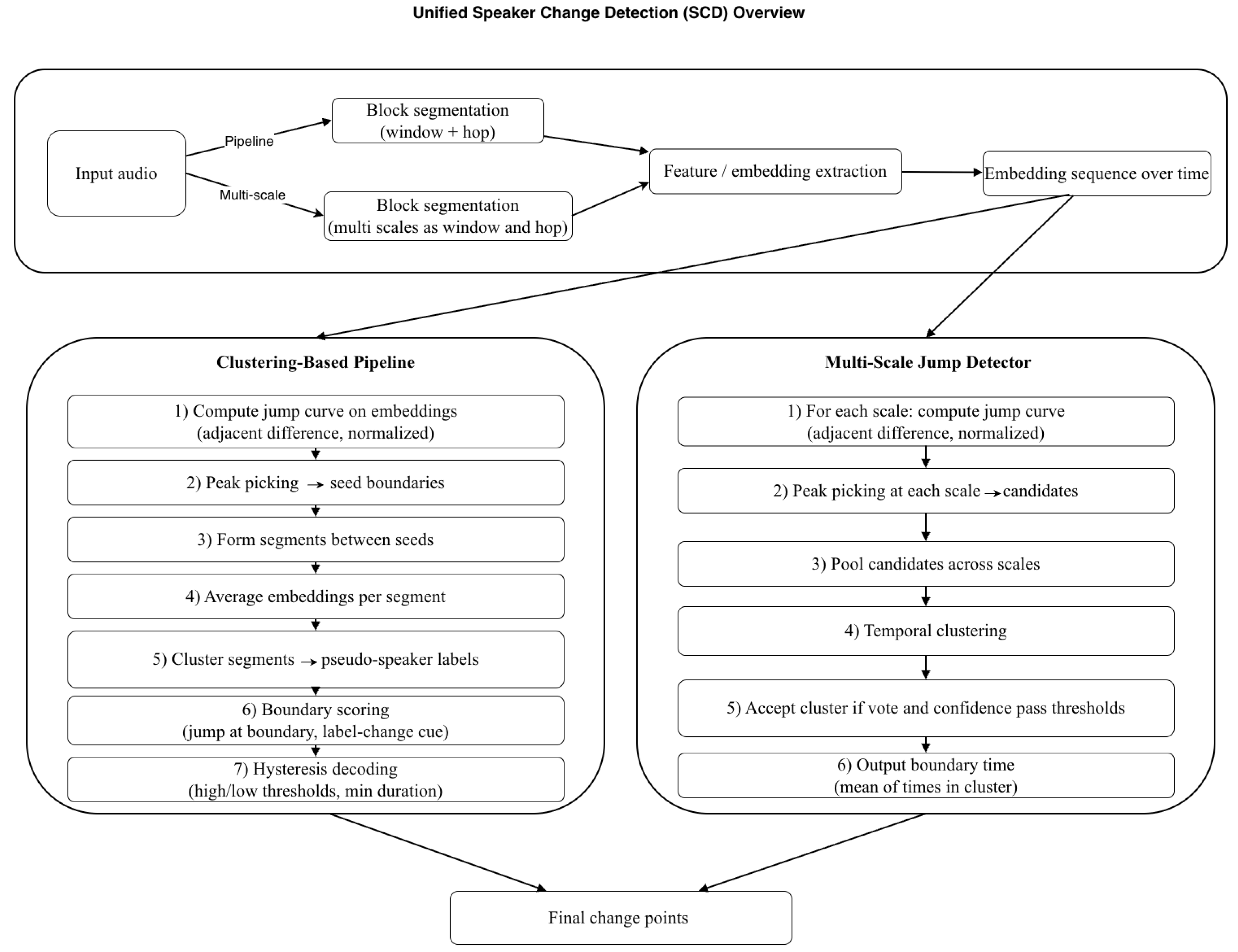
Figure 1 presents an overview of the proposed unified SCD framework and the two unsupervised back-end strategies compared in this study. Both methods share the same front-end (block segmentation and embedding extraction) and differ only in the back-end logic that converts the embedding sequence into boundary decisions.
The clustering-based pipeline combines local discontinuities with global structure. First, we compute a jump (novelty) curve on the embedding sequence and apply peak picking to obtain an initial set of “seed” boundaries, which partition the recording into short segments. For each segment, we compute a segment representation by averaging its block embeddings and then cluster these segment vectors (agglomerative clustering) to obtain pseudo-speaker labels. The final boundaries are scored using two cues: (1) the embedding jump at the segment boundary and (2) whether the pseudo-speaker label changes across the boundary. We then apply hysteresis thresholding (high/low thresholds) together with a minimum duration constraint to suppress short, low-confidence fluctuations.
The multi-scale detector reduces the sensitivity to a single window size by repeating jump-based detection at multiple time scales. We analyze the audio using a set of window lengths (e.g., 0.4 s, 0.8 s, and 1.6 s). At each scale, we compute a normalized jump curve and detect candidate peaks using a minimum distance rule and an adaptive quantile threshold. All candidates from all scales are pooled and temporally clustered. A cluster is accepted as a speaker change if it satisfies both a voting criterion (sufficient agreement relative to the number of scales) and a confidence criterion (mean peak strength). The final boundary time is taken as the mean timestamp of the accepted cluster.
3.1. Task Definition
Given a waveform
sampled at rate
, speaker change detection (SCD) aims to predict a set of boundary times,
at which the active speaker changes. During evaluation, a predicted boundary
is counted as a true positive if it falls within a tolerance collar of any reference boundary
:
where
s unless otherwise stated.
3.2. Acoustic Embeddings
The above-mentioned two methods are built upon a common foundation: high-dimensional acoustic embeddings. The audio is first segmented into overlapping blocks. An embedding model is then used to extract a feature vector for each block. The system supports several pluggable back-ends:
Log-Mel: The standard mean and standard deviation of log-mel spectrogram frames.
MFCC: The Mel-Frequency Cepstral Coefficient, a classic acoustic feature derived from the log-mel spectrogram.
ECAPA-TDNN: A speaker recognition model that provides a robust, fixed-dimension speaker embedding.
WavLM: A large-scale, pre-trained model that captures rich acoustic and contextual speech information.
wav2vec2: Another large-scale, pre-trained model that captures contextual speech representations.
We expect pre-trained self-supervised embeddings (WavLM and wav2vec2) to provide richer and more robust representations than handcrafted features (Log-Mel and MFCC), improving downstream analyses that rely on contextual and prosodic cues. Conversely, ECAPA-TDNN embeddings are expected to emphasize speaker identity and thus perform best in analyses primarily driven by speaker-specific characteristics.
3.3. Pipeline: Clustering-Based Approach
3.3.1. Seeding and Segmentation
The first stage operates on a single time scale defined by the block length w and hop size h. Let denote the embedding of the t-th block and let be the (normalized) jump curve computed from adjacent embeddings. We perform 1-D peak picking on with a minimum distance of blocks and a data-dependent height threshold (e.g., an upper quantile), obtaining peak indices . These peaks act as cutpoints and partition the recording into contiguous segments , where each segment contains the blocks between two consecutive cutpoints.
3.3.2. Segment-Level Embeddings and Clustering
For each segment
, we compute a segment-level embedding
by averaging the block embeddings within the segment:
where
is the embedding of segment
,
is the number of blocks in segment
,
t indexes blocks, and
is the embedding vector of block
t.
Given segment embeddings , we assign pseudo-speaker states by clustering in the embedding space. In our primary setting, we use agglomerative hierarchical clustering with cosine distance and average linkage. Starting from one cluster per segment, the algorithm iteratively merges the closest clusters until a cosine distance stopping threshold is reached. Each segment is thus assigned a discrete label , which is used as a global structural cue for speaker consistency over time.
This clustering step is suitable for unsupervised SCD because it provides a complementary prior to local jump/novelty peaks: if adjacent segments are assigned different pseudo-speaker labels (), a speaker change becomes more plausible, while stable labels can suppress spurious local fluctuations. The approach relies on standard embedding assumptions: segments from the same speaker form compact groups under cosine distance, whereas different speakers are more separated. Because the embeddings are high dimensional, distance-based behavior can be sensitive (e.g., threshold selection and noise/channel mismatch effects); segment-level averaging and L2 normalization help reduce within-segment variability, but clustering quality may still degrade when the embeddings are weak or heavily distorted, motivating our embedding comparison and robustness experiments.
In our implementation, each segment embedding is obtained by averaging the block embeddings within the segment followed by L2 normalization, and clustering is performed on these normalized vectors using cosine distance.
3.3.3. Boundary Scoring and Decoding
For each boundary between consecutive segments and , we define two scalar features.
(i) The segment boundary jump,
where
is the embedding jump at the boundary between
and
,
is the last block index of segment
,
is the first block index of segment
,
and
are the corresponding block embeddings, and
denotes the Euclidean norm.
(ii) The cluster change indicator,
where
indicates whether the cluster label changes across the boundary,
and
are the cluster labels of segments
and
, respectively, and
is the indicator function.
After normalizing
(e.g., min–max over
i), we combine both cues into a single boundary score:
where
is the final boundary score for the boundary between
and
,
and
are fixed weights (these hyperparameters were fine-tuned on the development set; see
Appendix A).
The score sequence is decoded into final change points using a 1-D hysteresis thresholding scheme with a high and a low threshold and a minimum duration (or minimum separation) constraint; equivalently, this can be viewed as a two-state decoder with asymmetric thresholds.
3.4. Multi-Scale Jump-Based Detector
3.4.1. Jump Curves at Multiple Time Scales
The multi-scale detector uses the same embedding model but operates at multiple analysis scales. We define a set of window lengths as follows:
where
is the set of analysis window lengths (scales),
is the
k-th scale in seconds, and
K is the number of scales.
For each scale,
, the waveform is segmented into blocks of length
w with a hop size of
. Let
denote the embedding of the
t-th block at scale
w. We compute a jump curve from adjacent embeddings as follows:
where
is the jump value at block index
t for scale
w,
is the embedding of block
t at scale
w, and
denotes the Euclidean norm. The sequence
is normalized to
before peak detection.
Local maxima are detected on
using a minimum distance and a percentile-based height threshold, yielding candidate peak indices
. These peaks correspond to candidate change times
(e.g., the start time of the peak block in seconds) with confidence scores, as follows:
here,
is the confidence (peak height) of the
m-th peak at scale
w, and
is its block index on the jump curve.
3.4.2. Cross-Scale Fusion by Grouping and Voting
All the candidate times from all the scales are pooled and sorted to obtain a combined set:
where
is the
n-th candidate boundary time (seconds),
is its confidence,
is the originating scale of this candidate, and
n indexes all the pooled candidates.
We then apply temporal grouping: candidates whose timestamps fall within a fixed window (e.g., 0.2 s) are assigned to the same group , where denotes a set of candidate indices n.
For each group
, we compute (i) a scale agreement score and (ii) a group confidence. Let
denote the set of distinct scales represented in
. Then, the scale agreement score is as follows:
where
is the fraction of scales that support group
,
is the number of distinct scales present in the group, and
is the total number of scales.
A confidence score is defined as the mean peak strength:
where
is the average confidence of candidates in group
,
is the number of candidates in the group, and
are the pooled candidate confidences from (
10).
A group is accepted as a change point if both criteria exceed the fixed thresholds (e.g.,
and
). The final boundary time is taken as the average timestamp of the group members:
Here, is the estimated speaker change time (seconds) for group , and are the candidate times within that group.
4. Experiments
4.1. Data Acquisition and Recording Conditions
We evaluate on the AMI Meeting Corpus [
29], which was recorded in instrumented meeting room environments using a synchronized, multi-stream acquisition setup that provided both close-talking and far-field audio. For completeness and reproducibility, we include an overview of the principal recording hardware and environmental conditions in Appendix
Table A1, covering the microphone types (headset, lapel, and table arrays), array geometry, the front-end and synchronization chain, and the relationship between the original capture format and the released waveform files [
30,
31,
32]. We used the IHM Mix-Headset recordings (single-channel mixed close-talking headset audio). The released waveform files used in the experiments have a sampling rate of 16 kHz.
4.2. Dataset Statistics
AMI provides an official development (DEV) and test split for meeting level evaluations. In this work, we do not use a separate training set because both approaches are unsupervised and do not require learning from annotated change points. All model comparisons are therefore reported on the AMI DEV and test sets, with meetings kept disjointed across the splits
Table 1 reports the per-recording statistics on the dev split. We show the recording duration (in seconds), the number of annotated speaker change boundaries (“#Boundaries”) and the boundary density in boundaries per minute (“Boundaries/min”). Dev contains 18 meetings ranging from ∼944 s to 2970 s. The boundary density spans 6.6–20.6/min, with IS1008b being the least conversationally active (6.62/min) and IB4010 the most (20.55/min). This spread reflects substantial heterogeneity across sessions, which we use to tune hyperparameters and check robustness.
Table 2 lists the same statistics for the TEST split (16 meetings). The durations range from ∼839 s to 2972 s. The boundary density is generally higher and broader than DEV, spanning 7.5–28.7/min: TS3003c is the calmest (7.54/min), while EN2002a is the most dynamic (28.70/min). The mixture of relatively quiet and highly interactive meetings makes this split a good stress test for change point detectors.
4.3. Computational Environment
To ensure the replicability of the research outcomes and provide transparency regarding the processing latency, all experiments were conducted on a high-performance workstation running Ubuntu 22.04 LTS. The hardware configuration and software stack are summarized in
Table 3.
The system is powered by an Intel Xeon Silver 4214R processor with a dual-socket configuration providing a total of 48 logical threads, which facilitates efficient parallelization during the multi-scale feature extraction stage. For model inference and gradient-intensive operations, we utilized an NVIDIA L40 GPU with 46 GB of VRAM and an NVIDIA A40 GPU with 46 GB of VRAM, ensuring that large-scale audio embeddings could be processed in high-capacity batches without memory bottlenecks. The system’s 376 GiB of RAM was instrumental in handling the simultaneous loading of multiple high-resolution jump curves across the AMI corpus.
The software environment was managed via a virtualized Conda environment to maintain dependency isolation. The core pipeline was implemented in Python 3.8.18, leveraging PyTorch 2.4.1 and CUDA 12.1 for GPU acceleration. Unsupervised clustering and statistical analyses were performed using Scikit-learn and SciPy, while Torchaudio and Torch-audiomentations provided the specialized machine learning instruments necessary for consistent audio signal processing.
4.4. Evaluation Metrics
To evaluate the performance with regard to speaker change point detection, a detected boundary is considered correct if it falls within a specified time tolerance (or “collar”) around a ground truth boundary. A standard tolerance of s is used unless otherwise specified. We also report sensitivity at .
To assess the performance of the approaches, several metrics are employed:
(i) The missed detection rate (MDR) measures the ratio of missed speaker change boundaries to the total number of ground truth boundaries:
(ii) The false alarm rate (FAR) measures the proportion of incorrect speaker change detections, calculated as the ratio of false positives to all non-change points:
Additionally, precision is used to indicate the accuracy of the detected speaker changes, recall (hit rate) assesses the ability to identify all true speaker changes, and the F1-score provides a balanced measure of precision and recall.
4.5. Experimental Design
The experiments are conducted on a standard benchmark dataset (the AMI Corpus) to ensure reproducible results. Although no supervised training is performed, both approaches include a small number of hyperparameters (e.g., peak picking thresholds, the minimum peak distance, the clustering threshold, and hysteresis/voting parameters). We selected these hyperparameters using the dev set, and then fixed the chosen values for all subsequent experiments. The final configuration was applied unchanged to the AMI test set; no test meetings were used for tuning or model selection.
4.6. Experiment 1: Acoustic Embedding Comparison
The goal of this experiment is to identify the most effective acoustic embedding for the segmentation task using two approaches. Five embedding types are considered: Log-Mel, MFCC, ECAPA-TDNN, WavLM, and wav2vec2. For fairness, all non-feature hyperparameters (e.g., for clustering algorithm) are held constant across runs. The performance is measured by the F1-score at a tolerance of . The best-performing embeddings under this criterion are selected for subsequent analyses.
4.7. Experiment 2: Evaluation Tolerance Sweeping
To characterize the tolerance sensitivity of the best-performing features, we run a tolerance sweep using the ECAPA-based pipeline. Specifically, we evaluate the system at three collar widths, and . For each tolerance, we compute the precision, recall, and F1-score, and compare how these metrics change as the collar widens. This analysis highlights which embedding is more accurate at tight boundary localization (small t) and which maintains more stable performance when near-miss detections are gradually forgiven (larger t).
4.8. Experiment 3: Clustering Method Comparison
This experiment evaluates the impact of different clustering algorithms within the pipeline, using the best-performing ECAPA-TDNN embedding. The clustering module is exchanged among the available algorithms, including Agglomerative, Spectral, and DBSCAN, while all other components and hyperparameters remain unchanged. We report the F1-score at for each method to quantify the influence of clustering choice on final detection accuracy.
4.9. Experiment 4: Analysis of Multi-Scale Settings
To better understand the behavior of the multi-scale detector, we conduct an ablation study on the choice of analysis scales and fusion strategy on the dev set. Concretely, we compare (i) a multi-scale detector using a window length of 0.8 s, (ii) two-scale variants combining 0.4 + 0.8 s and 0.8 + 1.6 s, and (iii) the full three-scale configuration 0.4 + 0.8 + 1.6 s used in the main experiments. The three window lengths are chosen to roughly cover short, medium, and long conversational units within meetings: 0.4 s is sensitive to rapid local changes (e.g., short backchannels), 0.8 s corresponds to typical short turns, and 1.6 s captures slower, more sustained speaker or topic shifts. This design allows us to test whether adding more scales always helps.
4.10. Experiment 5: Final Pipeline Comparison
Finally, we compare the two complete SCD approaches introduced in
Section 3 on the test set: (i) the clustering-based pipeline, configured with the best-performing embedding and clustering combination identified in Experiments 1 and 3 (ECAPA-TDNN with constrained agglomerative clustering) on the dev set, and (ii) the multi-scale jump-based detector using the same ECAPA embedding and evaluation protocol.
We evaluate the precision, recall, and F1-score at a tolerance of for both approaches on the AMI test splits to quantify their overall performance trade-offs.
4.11. Experiment 6: Evaluate Robustness
We further assess the robustness of the two unsupervised SCD methods under noisy conditions that approximate realistic deployment scenarios. Starting from the original AMI meeting dev recordings, we create three noisy test sets corresponding to low, medium, and high noise levels by adding zero-mean white Gaussian noise (WGN) to the waveform. For each recording, the noise is generated and scaled according to a predefined noise-to-signal power ratio (higher levels correspond to stronger noise) and then added sample-wise, with the resulting signal clipped to the range if necessary. For each noise level, we run both the clustering-based pipeline and the multi-scale detector with exactly the same hyperparameters as in the clean setting, and evaluate them using the standard metrics (precision, recall, F1, MDR, and FAR) at a 0.5 s tolerance. This setup allows us to quantify how each method trades off missed detections and false alarms as background noise increases, and to judge their suitability for real-world meeting scenarios with varying degrees of acoustic corruption.
We selected WGN for this evaluation to simulate broadband signal degradation and sensor noise in a controllable manner, without introducing the linguistic content found in babble noise. In the context of SCD, babble noise introduces competing speaker characteristics that can blur the definition of the foreground speaker, creating ambiguity regarding true change points. By using WGN, we isolate the model’s robustness to signal-to-noise ratio (SNR) reduction while maintaining a clear definition of the active speaker boundaries. It is important to note that the AMI corpus inherently includes realistic acoustic challenges, such as room reverberation, overlapping speech, and dynamic far-field artifacts. Therefore, the ’clean’ performance reported in
Section 5.5 already reflects the models’ capability to handle realistic meeting acoustics.
5. Results
5.1. Results of Acoustic Embedding Comparison
Table 4 summarizes the results of the pipeline on the development set with a 0.5 s tolerance. The ECAPA-TDNN embedding achieved a significantly higher F1-score (33.61) than all other features, driven by strong P (34.35) and R (32.89). WavLM was the clear runner-up, while the classic acoustic features (MFCC and Log-Mel) and the general-purpose wav2vec2 model showed considerably lower performance, particularly in recall.
We hypothesize that ECAPA-TDNN works best because it makes “steady” features for the same speaker/scene and shows a clear jump only when the speaker/scene really changes.
MFCC is more sensitive to small sound changes (like loudness or phonemes), so it fires inside segments and breaks them up. WavLM/wav2vec2 focus more on speech content (words/phones), so they often react at word changes, and, with their heavy context smoothing, can blur real speaker changes unless they are fine-tuned to speaker cues.
Table 5 presents feature comparison results of the multi-scale approach on development set. It can be observed, on the dev set (tol = 0.5 s), that the multi-scale detector works best with the ECAPA embedding, reaching 33.7% F1 with a relatively balanced precision (28.8%) and recall (40.4%). In contrast, WavLM achieves lower F1 (20.4%) and much lower recall, while wav2vec2, MFCC, and Log-Mel almost collapse in recall (<2%), with very low F1-scores despite low false alarm rates. This indicates that the effectiveness of the multi-scale method is highly dependent on the embedding, and ECAPA provides the most suitable representation in the current setting.
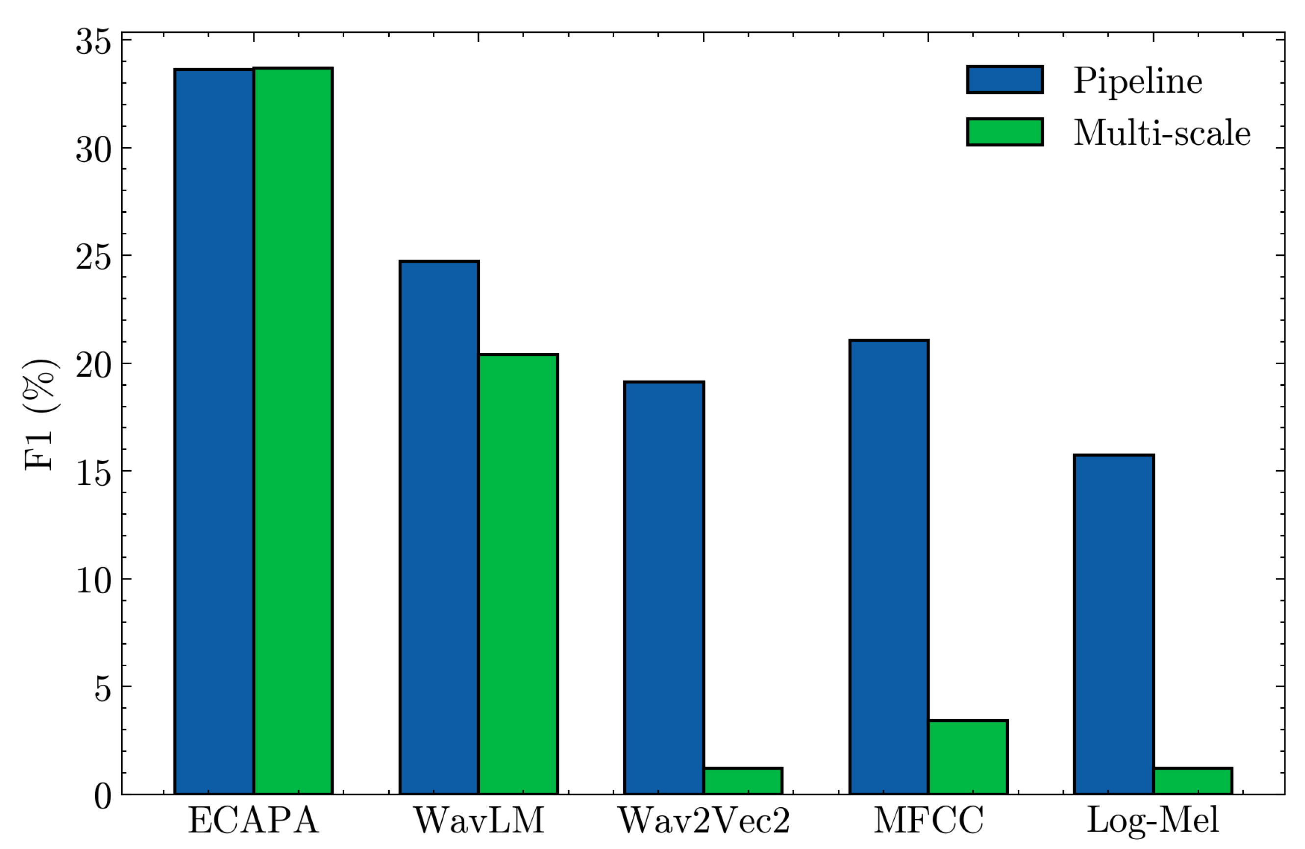
Figure 2 shows that the clustering-based pipeline outperforms the multi-scale detector for most feature types. With ECAPA embeddings the two methods are almost tied (both ≈ 34% F1), but for WavLM, wav2vec2, MFCC, and Log-Mel the pipeline is clearly better, while the multi-scale detector almost collapses for wav2vec2/MFCC/Log-Mel (F1 ≈ 1–4%). This indicates that the pipeline performs well across different embeddings, whereas the multi-scale method only works well when the embedding (ECAPA) already provides a very strong speaker-discriminative structure.
To demonstrate this behavior, we ran a small diagnostic experiment to understand why the multi-scale jump detector sometimes “collapses” (i.e., produces almost no speaker change boundaries) when we switch the embedding front-end. For each embedding type (ECAPA, WavLM, wav2vec2, MFCC, and log-Mel), we ran the same multi-scale detector on the development set using identical peak picking and the same fusion rules (temporal clustering + multi-scale voting + a confidence threshold). During this run, we logged two simple fusion-stage statistics: (1) the percentage of candidate peak clusters that survive the fusion gate (“pass rate”), and (2) the average confidence score of those peak clusters (“avg confidence”). We then averaged these statistics across recordings to produce the table. The results (see
Table 6) show a clear pattern: ECAPA generates strong, well-separated peaks, so a substantial fraction of candidates pass fusion (pass rate 24.8%) and their confidence is high (0.81), meaning the detector remains active. WavLM is intermediate (pass rate 8.8%; confidence 0.65), indicating partial degradation rather than total failure. In contrast, MFCC, log-Mel, and wav2vec2 produce much weaker peak evidence under the same settings, so fusion rejects almost everything (pass rates 2.2%, 0.4%, and 0.4%, with confidence around 0.46–0.57). This explains the observed “collapse”: with these embeddings, the fusion stage becomes overly conservative and suppresses nearly all detections, leading to the near-zero predicted change points.
Under the same clustering algorithm (agglomerative) and evaluation tolerance (0.5 s), ECAPA features significantly outperformed other custom/handcrafted features for both approaches.
Based on this, we used ECAPA+Agglomerative as the primary configuration for subsequent development and test set validation.
5.2. Results for Tolerance Sweeping
We compare the pipeline with the multi–scale detector under different collar tolerances (0.25/0.5/0.75 s). The results are presented in
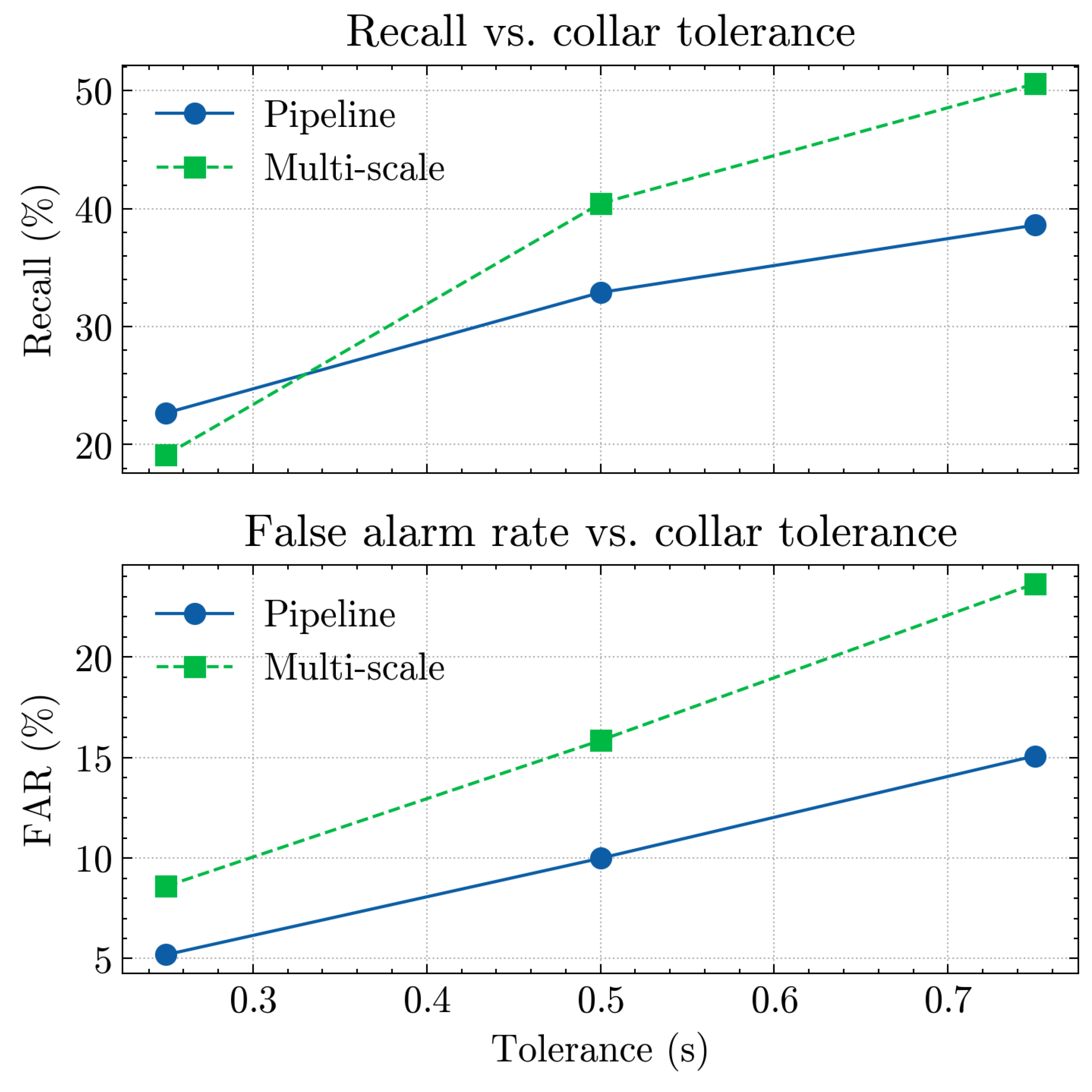
Table 7. At the strict 0.25 s collar, the pipeline clearly outperforms the multi–scale variant in terms of precision, recall, and F1 (23.17% vs. 15.93%), while also achieving a lower false alarm rate (5.19% vs. 8.60%), indicating a more conservative and cleaner segmentation. At the standard 0.5 s collar, both systems obtain almost identical F1-scores (33.6%), but the multi–scale detector achieves a substantially higher recall (+7.6 pp, 40.44% vs. 32.89%) at the cost of a higher FAR (+5.9 pp). With a more relaxed 0.75 s collar, the multi–scale approach further improves F1 (42.12% vs. 39.44%) and recall (50.58% vs. 38.60%), again trading off against an increased FAR (23.65% vs. 15.08%). Overall, the multi-scale detector is more recall-oriented and tends to over-segment, whereas the pipeline is more conservative with fewer false alarms.
Figure 3 illustrates how the pipeline and the multi–scale detector behave under different collar tolerances (0.25 s, 0.5 s, and 0.75 s). As the tolerance increases, both approaches gain recall but also incur higher FAR. The multi–scale detector achieves higher recall than the pipeline, especially at 0.5 s and 0.75 s, but at the cost of more false alarms, while the pipeline remains more conservative with lower FAR.
5.3. Result with Various Clustering Algorithms
Experiment 3 evaluated the impact of different clustering algorithms within the pipeline, using the best-performing ECAPA-TDNN embedding. As shown in
Table 8, the choice of algorithm is critical to the pipeline’s performance.
The constrained agglomerative clustering method was the only effective algorithm, achieving an F1-score of 33.61. This result was stable across various distance thresholds (0.55 to 0.65). In sharp contrast, both spectral clustering and DBSCAN failed catastrophically. While they achieved high precision (37.32% and 37.03%), their recall was exceptionally low (11.21% and 2.02%, respectively). This indicates that these methods are far too conservative for this task, correctly identifying a few boundaries but missing the vast majority, rendering them unsuitable for this pipeline.
5.4. Results of Analysis of Multi-Scale Settings
Table 9 summarizes an ablation on the choice of analysis scales for the ECAPA-based multi-scale detector on the dev set (tol = 0.5 s). Using a single scale of 0.8 s already gives a reasonably balanced operating point (F1 = 35.6%) with moderate recall (44.4%) and a relatively low false alarm rate (FAR = 16.7%). Adding a shorter 0.4 s scale (0.4 + 0.8) dramatically boosts recall to 83.3% but at the cost of a relatively high FAR (51.5%), indicating that the additional sensitivity mainly manifests as many extra false positives. Using a longer auxiliary scale (0.8 + 1.6) yields a more conservative detector with a slightly lower F1 (33.3%) and higher FAR than the single-scale multi-scale detector. The full three-scale configuration (0.4 + 0.8 + 1.6) sits between these extremes: it slightly reduces the F1 compared to the best single-scale setting, but achieves the lowest FAR (15.9%), suggesting that the additional scales act more as regularizers that trade some recall for fewer false alarms.
5.5. Results on Test Set
Table 10 reports per-recording performance for the clustering-based pipeline and the multi-scale detector on the test set (tol = 0.5 s). Overall, the pipeline operates in a more conservative regime: it achieves higher average precision (34.9% vs. 20.4%) and a slightly higher average F1 (34.4% vs. 32.1%), with a much lower average false alarm rate (FAR 10.0% vs. 50.0%). In contrast, the multi-scale method aggressively favors recall, reaching an average recall above 82% on all recordings, which corresponds to a much lower missed detection rate (MDR 17.5% vs. 64.6% for the pipeline), but this comes at the cost of relatively high false alarm rates on almost every file. The per-file results show the same pattern: the multi-scale detector substantially increases recall and reduces MDR on all meetings, while the pipeline provides more balanced precision–recall trade-offs and more stable FAR across sessions.
5.6. Results of Robustness
Table 11 summarizes the behavior of the two methods under three noise levels. For low and medium noise, the multi-scale detector retains relatively high recall (75–85%) but at the price of extremely high false alarm rates (FAR 50–64%), so its overall error is dominated by false positives. In contrast, the pipeline operates in a more conservative regime with much a lower FAR (about 8–12%) and a slightly higher F1 in these two conditions, but its missed detection rate (MDR ≈ 59–73%) is still high, indicating that many true changes are not detected.
Under high noise, both methods become problematic in different ways. The multi-scale detector reduces FAR to about 16% but its MDR increases to nearly 64%, so the total error remains large even though the F1 stays around 28%. The pipeline almost stops working as a detector: its recall drops to about 0.7% and MDR approaches 99%, meaning that it produces almost no change points at all and the low FAR (≈0.1%) is achieved only because the system rarely fires. From the joint perspective of MDR and FAR, this operating point is clearly undesirable. Overall, as noise increases, the multi-scale method mainly trades precision for recall, whereas the pipeline tends to become overly conservative and can fail to function as a useful SCD system under high-noise conditions.
5.7. Comparing with Other Unsupervised Approaches
Table 12 compares two ECAPA-based models with classic unsupervised SCD baselines from [
1] in terms of MDR and FAR (lower is better). All methods are evaluated on the AMI test set. BIC- and KL-based methods with hand-crafted features typically operate around MDR ≈ 39–47% and FAR ≈ 48–60%. The pipeline model is very conservative: it achieves a much lower FAR (9.98%) than all BIC/KL systems, but with a high MDR (64.95%). In contrast, the multi-scale model attains the lowest MDR in the table (18.24%), showing strong sensitivity to changes, at the price of a FAR (49.01%) comparable to the classic unsupervised approaches.
It is important to note that the feature choices for the baseline methods reflect their specific mathematical constraints. Classic BIC and KL approaches typically rely on parametric Gaussian modeling and covariance estimation, which perform optimally with lower-dimensional inputs (such as MFCCs or Chroma) and struggle with the high dimensionality of modern embeddings due to estimation instability [
1]. In contrast, the pipeline and multi-scale models are designed to exploit high-dimensional representations. To ensure a rigourous comparison, the baseline results in
Table 12 are derived from the top-three performing feature configurations identified in prior work [
1], representing the optimal operating regime for these classic statistical methods.
6. Discussion
6.1. Impact of Embedding Choice on Performance
The embedding comparison shows that representation choice can dominate method choice. On the dev set, the ECAPA-based approach produces the strongest overall performance for both paradigms (the pipeline F1 is 33.61; the multi-scale F1 is 33.67), while several alternatives degrade substantially. Most notably, the multi-scale detector nearly collapses in recall for wav2vec2/MFCC/log-Mel (recall ), despite low FAR, indicating that multi-scale peak fusion cannot compensate for embeddings that do not yield stable speaker-discriminative discontinuities. By contrast, the pipeline degrades more gracefully across features, suggesting that its structure-building step (segment averaging + clustering + hysteresis) acts as a partial stabilizer when local novelty curves are noisy or speaker cues are weak.
The qualitative hypothesis is also consistent with these trends: ECAPA appears to provide “steadier” speaker-relevant representations that only jump when speakers truly change, whereas MFCC is sensitive to within-speaker variations (phonetic/loudness) and SSL encoders may emphasize content and context smoothing in ways that blur speaker boundaries unless adapted for speaker cues. These results suggest that performance differences are not merely due to the back-end decision rule, but are strongly shaped by the embedding’s inductive bias, i.e., whether the representation emphasizes speaker identity versus phonetic/content variation, which is critical for reliable unsupervised boundary detection. The weak performance of WavLM/wav2vec 2.0 features in our unsupervised SCD back-ends also suggests a practical implication: although SSL encoders are powerful general-purpose speech representations, their pre-training objectives primarily emphasize content and contextual prediction, and the resulting embeddings are not necessarily optimized for speaker discriminability at short time scales. Consequently, if the goal is strong SCD performance in practice with jump-based or clustering-based unsupervised detectors, it may be beneficial to adapt these SSL encoders toward speaker-relevant cues. This can be achieved by fine-tuning (or lightweight adaptation) with speaker-oriented objectives (e.g., speaker classification/verification losses), diarization/segmentation supervision when available, or weakly supervised/self-training schemes that use pseudo-speaker labels obtained from clustering. Such adaptation is expected to increase between-speaker separability and reduce within-speaker variability, producing clearer and more stable embedding discontinuities that downstream unsupervised SCD rules can exploit.
6.2. Why the Two Paradigms Occupy Complementary Regimes
On the test set (0.5 s collar) (
Table 10), the pipeline achieves higher precision (34.9% vs. 20.4%) and dramatically lower FAR (10.0% vs. 50.0%), while the multi-scale detector achieves much higher recall (82.5% vs. 35.4%) and lower MDR (17.5% vs. 64.6%). The contrasting error profiles also reflect a fundamental modeling difference: the multi-scale detector is driven primarily by local discontinuities, whereas the pipeline is driven by global (sequence-level) consistency.
Multi-scale jump detection evaluates left–right embedding mismatch within short contexts and triggers boundaries at prominent peaks; even when multiple context lengths are fused, the decision mechanism remains local and therefore highly sensitive to transient embedding fluctuations.
By contrast, the pipeline first induces a longer-range structure by clustering embeddings into pseudo-speaker states across the recording and then decodes boundaries under temporal constraints (e.g., hysteresis and minimum duration rules). This introduces an implicit global prior that favors temporally stable speaker assignments and suppresses rapid back-and-forth switching, which typically reduces false alarms but can also merge short turns and increase the missed detections. In this sense, the two paradigms embody complementary inductive biases, local contrast vs. global consistency, helping to explain why they occupy different regions of the miss–false alarm trade-off.
6.3. Effect of Collar Tolerance
Collar tolerance determines how strictly boundary timing is judged: a smaller collar requires predicted change points to fall closer to the reference time to be counted as correct. With a tight collar (
s), the pipeline performs best, achieving a higher F1 (23.17% vs. 15.93%) while also producing fewer false alarms (FAR 5.19% vs. 8.60%) (
Table 7). This indicates that, in our setting, pipeline not only triggers fewer boundaries, but its predicted boundaries are also better time-aligned with the reference. A plausible explanation is that the pipeline’s clustering and temporal constraints suppress short-lived fluctuations and reduce boundary jitter, leading to more stable and better-localized change estimates.
At the standard collar ( s), both methods reach essentially the same F1 (33.61% vs. 33.67%), but they do so via different operating points: the multi-scale detector yields substantially higher recall (40.44% vs. 32.89%) while incurring a higher FAR (15.85% vs. 9.99%). When the collar is further relaxed ( s), the multi-scale detector benefits more from the additional tolerance and overtakes the pipeline in F1 (42.12% vs. 39.44%) and recall (50.58% vs. 38.60%), again at the cost of a noticeably higher FAR (23.65% vs. 15.08%).
Overall, increasing the collar widens the set of “acceptable” detections for both approaches, so recall increases for both, yet the multi-scale detector gains recall more aggressively while the pipeline remains more conservative with consistently lower FAR. Interpreted through the lens of model bias, this pattern is consistent with multi-scale jump detection producing many near-boundary candidates (high sensitivity but higher jitter/over-segmentation), whereas the Pipeline favors fewer, temporally consistent cuts (cleaner segmentation but more misses when turns are short or ambiguous).
6.4. Effect of Scale Ablation
Table 9 shows that adding analysis scales is not uniformly beneficial; instead, the scale set mainly controls the detector’s sensitivity. Using a single 0.8 s scale already provides a balanced operating point (precision 29.69%, recall 44.40%, and F1 35.58%) with a moderate FAR of 16.71%. When a shorter 0.4 s scale is added (0.4 + 0.8), recall jumps sharply to 83.29%, but FAR increases dramatically to 51.52%, and F1 drops to 32.83%.
This indicates that the extra short-scale sensitivity largely manifests as many additional false positives rather than consistently improving usable boundary hypotheses. Adding a longer auxiliary scale (0.8 + 1.6) yields a more conservative behavior (F1 33.32%; FAR 20.94%) that does not improve over the best single-scale setting. The full three-scale configuration (0.4 + 0.8 + 1.6) sits between the extremes: it reduces recall relative to 0.8 alone (40.44% vs. 44.40%) and slightly lowers F1 (33.67% vs. 35.58%), but achieves the lowest FAR among the tested configurations (15.85%).
Overall, these trends suggest that multi-scale fusion should be treated as a tunable design choice: adding shorter scales can prioritize recall at the cost of over-segmentation, while adding longer scales can act as a regularizer that trades some recall for fewer false alarms.
6.5. Robustness Under Additive Noise Exposes Failure Modes
The noise study highlights different breakdown behaviors. Under low/medium noise, the multi-scale detector maintains very high recall (75–85%) but becomes dominated by false alarms (FAR 50–64%), while the pipeline remains conservative (FAR about 8–12%) but still misses many changes. Under high noise, the pipeline essentially stops firing (recall , MDR ), while the multi-scale detector retains moderate recall but still suffers substantial error.
This result demonstrates that two unsupervised paradigms do not merely degrade “a bit” under corruption, they fail in qualitatively different ways. That insight is valuable for downstream diarization/meeting systems because practitioners often prefer a controllable failure mode (e.g., higher FAR but stable recall) over a silent failure (near-zero recall).
6.6. Implications for Practical Deployment
The robustness trends suggest that, in practical diarization and meeting processing pipelines, the preferred SCD back-end depends on which failure mode is more acceptable. If downstream clustering/tracking is sensitive to fragmented turns (or if manual review cost is high), a conservative pipeline-style regime is often preferable because it maintains a substantially lower FAR, producing cleaner segmentations even if more true changes are missed. Conversely, if the downstream system can absorb extra candidate boundaries (e.g., via later merging or resegmentation), the multi-scale detector can be advantageous because it preserves high recall and avoids “silent” failures where true speaker switches are largely missed, albeit at the cost of over-segmentation.
A second implication is that representation quality can be a limiting factor for these unsupervised rules. In particular, the multi-scale detector is effective only when embeddings yield consistent speaker-discriminative discontinuities; when this condition is not met, tuning peak picking or fusion heuristics is unlikely to recover performance. This suggests that, for SSL encoders such as WavLM or wav2vec 2.0, speaker-oriented adaptation (e.g., fine-tuning with speaker/diarization objectives or pseudo-label self-training) may be necessary to obtain strong practical performance with both jump-based and clustering-based unsupervised SCD.
Table 13 presents a computational complexity analysis of the two approaches measured on on NVIDIA L40 GPU. The clustering-based pipeline demonstrates superior efficiency with a real-time factor (RTF) of approximately 0.025, indicating that it processes audio roughly 40 times faster than real-time. This efficiency stems from its single-pass embedding extraction and low-overhead hierarchical clustering.
In comparison, the multi-scale detector operates with an RTF of approximately 0.090 (about 11 times faster than real-time). The increased computational cost is primarily due to the redundancy of extracting embeddings and computing jump curves across multiple temporal scales (e.g., 0.4 s, 0.8 s, and 1.6 s) before fusion. Nevertheless, both methods achieve RTFs well below 1.0, confirming their suitability for practical deployment in both offline batch processing and streaming scenarios.
7. Conclusions
In this paper, we study unsupervised speaker change detection in meeting recordings under a unified embedding-based framework. We use a common front-end with block segmentation and pre-trained embeddings to compare two structural paradigms: a clustering-based pipeline with hysteresis decoding, and a multi-scale jump-based detector that aggregates embedding discontinuities across multiple time scales. Both methods are assessed on the AMI corpus using a consistent protocol for tolerance, evaluation metrics, and data splits.
The experimental study covered several dimensions. First, we performed a feature/embedding comparison for both methods using ECAPA, WavLM, wav2vec 2.0, MFCC, and log-Mel features. Second, we ran a head-to-head comparison of the pipeline and multi-scale detector on dev and test sets, including per-recording analyses. Third, we conducted an ablation on the multi-scale configuration, varying window sets (single-scale 0.8 s, two-scale 0.4 + 0.8 and 0.8 + 1.6, and three-scale 0.4 + 0.8 + 1.6). Fourth, we evaluated robustness to additive white noise at low, medium, and high levels. Finally, we compared against classic unsupervised SCD baselines (BIC/KL with hand-crafted features) using common MDR/FAR metrics.
The results lead to several key findings. (1) Embedding choice is critical, especially for the multi-scale detector: ECAPA delivers the best F1, while wav2vec2, MFCC, and log-Mel cause the multi-scale approach to almost collapse in recall, whereas the pipeline remains more stable across embeddings. (2) The two methods occupy complementary operating regimes. On test meetings, the pipeline yields higher precision and much lower FAR, but with relatively high MDR; the multi-scale detector achieves relatively high recall (low MDR) at the expense of many false alarms. The per-file results confirm this pattern across all sessions. (3) The multi-scale ablation shows that a single 0.8 s scale already gives strong and balanced performance; adding a shorter 0.4 s scale dramatically boosts recall but drives FAR up, while the three-scale configuration slightly reduces F1 yet delivers the lowest FAR, suggesting that additional scales mainly act as regularizers that can be tuned to the desired precision–recall trade-off. (4) Under increasing noise levels, both methods become less reliable, but in different ways: for low and medium noise the multi-scale detector retains relatively high recall at the cost of an extremely high FAR (errors dominated by false alarms), while the pipeline stays usable with much lower FAR but still high MDR; under high noise, the multi-scale detector loses recall and still has substantial FAR, and the pipeline almost stops detecting changes at all (near-zero FAR only because almost all true change points are missed). (5) Compared to BIC/KL-based unsupervised SCD with hand-crafted features, the ECAPA-based models can reach substantially lower MDR (multi-scale) or substantially lower FAR (pipeline), showing that modern embeddings plus simple structural priors can outperform classic feature–statistic combinations along different ends of the error trade-off.
These observations suggest several directions for future work. Based on the complementary operating regimes identified in this study, a concrete hybrid design could be implemented as a ’Propose-and-Verify’ system. In this architecture, the multi-scale jump detector (configured for high sensitivity) would serve as the ’Proposer,’ generating a dense set of candidate change points to minimize missed detections. These candidates would then define the initial segmentation for the clustering-based pipeline, which acts as the ’Verifier.’ By performing agglomerative clustering on these segments, the system would validate candidates based on global speaker consistency rejecting boundaries that do not correspond to a switch in pseudo-speaker labels. This approach would theoretically combine the multi-scale detector’s ability to capture short, rapid turns with the pipeline’s robustness against spurious, transient noise. Another direction is to introduce lightweight supervision or semi-supervised calibration on top of the unsupervised scores, to better control the MDR–FAR trade-off without requiring large amounts of annotated change points. Finally, extending the analysis to more diverse conversational domains and exploring end-to-end architectures that retain the interpretability of jump- and cluster-based features would further bridge the gap between traditional unsupervised pipelines and fully supervised SCD systems.