A Low-Complexity Versatile Beamforming Method for Multiple Parametric Arrays

Abstract

The application of multiple parametric arays (MPAs) has been increasingly prominent in recent years due to the high directivity of parametric arrays. However, existing beamforming methods for MPAs are limited to special scenarios, such as narrow-edged beamforming, or have high complexity, such as requiring numerous acoustic transfer function (ATF) identifications. This paper proposes a low-complexity versatile beamforming method based on the transitive relationship among ATFs. For N parametric arrays, the number of identified ATFs can be reduced from N² to N through interpolation and flipping. Moreover, by neglecting the less affected part in the acoustic field structure, the number of identified ATFs can be reduced to less than N. On the basis of ATF matrix estimated, the desired acoustic field can be generated by optimizing the emission weight coefficient. The accuracy of ATF estimation is verified through the precise reconstruction of the acoustic field. Even when the number of identified ATFs does not exceed N, the desired acoustic field of different types of beam patterns can be formed correctly. The beamforming effects of MPAs confirm the low-complexity and versatility of the proposed method, offering a highly feasible solution for acoustic field control.

1. Introduction

By adjusting the transmit weight coefficient of each array element, the desired sound field distribution can be generated, known as transmit beamforming. The technology is widely used in audio reproduction [1], tissue harmonic imaging [2], target tracking [3], underwater acoustic communication [4], and other fields. However, according to the Rayleigh integral, low-frequency sounds such as audio and long-distance propagation underwater acoustic signals necessitate a large radiation surface to achieve high directivity. In response to this challenge, Westervelt [5] introduced the concept of parametric acoustic arrays. Thanks to the compact virtual source generated by the nonlinear acoustic effect in the fluid, the parametric array can form a highly directional low-frequency sound while maintaining a small aperture size. This unique property enables the miniaturization design of a high-resolution low-frequency acoustic excitation system. According to the relationship of the Rayleigh integral, conventional sound sources need a transmitting transducer of a considerable size to achieve the function of high-resolution low-frequency acoustic excitation. This cost is unacceptable in most cases, while a parametric array solves this problem through its unique property. In audio engineering [6], the parametric array has the applications of low leakage active noise control, personal communication, etc. In underwater acoustic engineering [7], the parametric array is often applied to sub-bottom profilers, covert underwater communication, the detection of buried targets, etc. Nonetheless, the beam pattern formed by individual parametric arrays is hard to regulate.

To improve the flexibility of system operation, recent research [8,9,10,11] has been dedicated to configuring multiple parametric arrays (MPAs) in specific formations. By individually controlling emission parameters of MPAs, beamforming of various types can be achieved, such as beamsteering, narrow-edged, vortex beam, and constant beamwidth. Since MPAs maintain the unique property of parametric arrays, their applications are the same. Due to the high control flexibility, MPAs allows the location of a target to be variable, such as with seafloor sediment mapping and communication objects with non-fixed positions. Zhu et al. [11] achieved beamsteering and sidelobe suppression of an audible sound when the Nyquist criterion was not satisfied. The beamsteering algorithm adopted minimum variance distortionless response to enhance the directivity. Geng et al. [8] proposed a narrow-edged beamforming method for parametric loudspeakers, which have narrower beamwidth generation compared to conventional parametric loudspeakers. This method involves controlling the phase of high-frequency waves at the edges to induce constructive interference of the difference-frequency waves at the edge of the main lobe. Jiménez et al. [9] achieved the formation of a vortex beam by arranging MPAs on a helicoidal curved surface. Benefitting from the high directivity of the parametric array and the focal point of the curved surface, the structure of the vortex beam was at the sub-wavelength scale. Such vortex beams generated by parametric arrays have potential application in underwater acoustic communications [12,13]. Constant beamwidth beamforming is essential to minimizing sound distortion along the off-axis direction. Yang et al. [14] devised a constant beamwidth beamformer based on Chebyshev weighting and validated it through simulation by a product model. However, the product model was not quite precise for the calculation of directivity. Zhu et al. [10] proposed an optimal audio beam pattern synthesis method, utilizing the more accurate convolution model [15] to create a convex optimization objective function. The capability of constant beamwidth control was confirmed through experiments. As for the grating lobe suppression, arranging MPAs in a pseudo-random configuration is effective, such as hyperuniform disordered [16]. Furthermore, the acoustic field distribution on the radiator axis is also of concern while beamforming is performed on circumferential positions. For instance, when there are reflectors at distal locations, the audible area can be restricted to the near field by forming a length-limited audio beam. Skinner et al. [17] demonstrated a length-limited parametric array in the outdoor experiment. The length limitation in audio radiation along the radiator axis was observed, arising from destructive interference in the far field. While utilizing a pair of high-frequency carrier waves of the same frequency [18], the intermodulation distortion of a length-limited parametric array can be mitigated.

The studies mentioned above could achieve beamforming in specific scenarios, yet they lacked versatility. To alleviate this limitation, a nonlinear sound field control framework [19] was constructed by identifying the acoustic transfer function. Considering the nonlinear coupling between channels, the number of acoustic transfer functions (ATFs) to be identified in the framework is the square of the MPA number. The high complexity of identification systems renders the executing process of beamforming cumbersome. This study proposes a low-complexity versatile beamforming method for multiple parametric arrays. This article is outlined as follows. The acoustic field structure of MPAs is analyzed in Section 2.1 to characterize the ATF. Meanwhile, a numerical model of acoustic field structure unit is established based on Gaussian beam expansion. Then, the framework of the low-complexity versatile beamforming method is developed in Section 2.2. By leveraging the transitive relationship between ATFs, the number of ATFs could be significantly reduced. On the basis of the ATF matrix estimated, the emission weight coefficient was optimized to realize the beamforming of MPAs. Section 3.1 details the numerical model setup, which also verified the high calculation accuracy of the model. Finally, the effectiveness of ATF estimation and beamforming is validated through the exact and desired acoustic field in Section 3.2 and Section 3.3.

2. Theory

2.1. Acoustic Field Structure of Multiple Parametric Arrays

The Westervelt equation under the quasi-linear approximation assumption [20] can be written as

$${\nabla }^2{p}_d\left(\mathbf{r}\right)+{k_d}^2{p}_d\left(\mathbf{r}\right)={\displaystyle \frac{\beta {{\omega }_d}^2}{{\rho }_0{c_0}^4}}{p}_1\left(\mathbf{r}\right){p_2}^{\ast }\left(\mathbf{r}\right),$$

(1)

where $p_d$ denotes the difference–frequency acoustic field. $\beta$ is the nonlinear coefficient, $c_0$ is the speed of sound, and ${\rho }_0$ is the fluid density. $\mathbf{r}$ denotes the coordinate vector of the field point; $p_i$ denotes the high-frequency wave acoustic field at the frequency $f_i$, where the subscripts i represent the serial number of high-frequency; and $i=1,2$, $f_1-f_2=f_d$. ${\omega }_d$ and $k_d$ are the angular frequency and the wave number of the difference–frequency wave. Superscript “∗” represents the conjugation.

Equation (1) is a nonhomogeneous Helmholtz equation. By introducing the Green’s function $-e^{\mathrm{j}{k}_d{d}_v}/\phantom{e^{\mathrm{j}{k}_d{d}_v}4\pi d_v}4\pi d_v$, the difference–frequency acoustic field of the MPAs can be written in the form of virtual source integral:

$$p_d\left(\mathbf{r}\right)=-{\displaystyle \frac{\beta {{\omega }_d}^2}{4\pi {\rho }_0{c_0}^4}}{\int }_{z_v=0}^{\infty }{\int }_{y_v=-\infty }^{\infty }{\int }_{x_v=-\infty }^{\infty }{p}_1\left({\mathbf{r}}_{\mathbf{v}}\right){p_2}^{\ast }\left({\mathbf{r}}_{\mathbf{v}}\right){\displaystyle \frac{{\mathrm{e}}^{\mathrm{j}{k}_d{d}_v}}{d_v}}\mathrm{d}{x}_v\mathrm{d}{y}_v\mathrm{d}{z}_v,$$

(2)

where ${\mathbf{r}}_{\mathbf{v}}$ denotes the coordinate vector of the virtual source point and $d_v$ represents the distance $\left|\mathbf{r}-{\mathbf{r}}_{\mathbf{v}}\right|$.

Setting the number of MPAs as N, the acoustic field structure of high-frequency wave can be expressed as

$$p_i=\sum _{\Gamma =1}^N{p}_i^{\left(\Gamma \right)},$$

(3)

where the superscript $\Gamma$ denotes the serial number of the parametric array in MPAs.

Broadly speaking, the difference-’frequency wave acoustic field can be referred to as the scattering of sound by sound (SSS). For the parametric array numbered $\Gamma$, $\Lambda$, the acoustic field structure of difference’-frequency wave is a sum of self SSS and mutual SSS, as shown in Figure 1. Self SSS is generated by an emission transducer through self-interaction, e.g., $p_d^{\left(\Gamma ,\Gamma \right)},p_d^{\left(\Lambda ,\Lambda \right)}$. Mutual SSS is generated by different emission transducers through mutual interaction, e.g., $p_d^{\left(\Gamma ,\Lambda \right)},p_d^{\left(\Lambda ,\Gamma \right)}$. The first digit of superscript of $p_d$ represents the serial number of the parametric array that transmits the sound signal with $f_1$, while the second represents that of $f_2$. Consequently, the difference-’frequency wave sound pressure of N parametric arrays can be represented by the following expression:

$$p_d=\sum _{\Gamma =1}^N\sum _{\Lambda =1}^N{p}_d^{\left(\Gamma ,\Lambda \right)}.$$

(4)

Figure 2 shows the schematic of multiple parametric arrays in beamforming scenarios. The shape of the parametric array is a rectangle with dimensions of $2a_x\times 2a_y$. MPAs are evenly arranged along the x-axis with a spacing of d. The acoustic field control positions are located at a distance z from the origin, arranged along the x-axis with a spacing of $\Delta x$. The angle between each acoustic field control positions and the origin is denoted by $\theta$. The acoustic field can be modeled by Equation (2), which is a triple integral with substantial computational complexity. Paraxial approximation and Gaussian function expansion can be applied to reduce the integration dimension. Paraxial approximation of $d_v$ in Equation (2) is performed along the z-axis.

$$d_v\approx \left|z-z_v\right|+{\displaystyle \frac{{\left[x-x_v\right]}^2+{\left[y-y_v\right]}^2}{2\left|z-z_v\right|}}.$$

(5)

The phase term of ${\displaystyle \frac{{\mathrm{e}}^{\mathrm{j}{k}_d{d}_v}}{d_v}}$ in Equation (2) is approximated by the right item in Equation (5), while the amplitude term is approximated by $\left|z-z_v\right|$. While simplifying the calculation, the paraxial approximation limits the effective model space to a small angle. However, due to the complexity of virtual source integral Equation (2), the effective angle range is affected by various factors: the directivity of high-frequency waves, difference frequency, and field point distance. In Section 3.1, we quantitatively analyze the modeling accuracy of paraxial approximation in the numerical model setup.

The vibration velocity distribution on the surface of the parametric array numbered $\Gamma$ is expanded by the Gaussian functions:

$$u_i^{\left(\Gamma \right)}(x_s,y_s)\approx U_i^{\left(\Gamma \right)}\sum _{m_i=1}^M{A}_{m_i}\exp \left\{-B_{m_i}{\left[x_s-d_{\Gamma }\right]}^2/\phantom{{\left[x_s-d_{\Gamma }\right]}^2{a}_x^2}{a}_x^2\right\}\times \sum _{n_i=1}^M{A}_{n_i}\exp \left(-B_{n_i}{y}_s^2/\phantom{y_s^2{a}_y^2}{a}_y^2\right),$$

(6)

where $A,B$ are the Gaussian expansion coefficients, which can be obtained by optimizing the root mean square error of exact distribution and Gaussian expansion distribution [21], and $U_i^{\left(\Gamma \right)}$ is the vibration velocity. M denotes the number of the Gaussian functions. To balance the complexity and accuracy of the calculation, M usually takes a value of around ten [20].

Substituting Equations (5) and (6) into Equation (2), the calculation formula for the acoustic field structure unit is simplified to a single integral:

$$\begin{array}{c}{p}_d^{(\Gamma ,\Lambda )}(x,y,z)={\displaystyle \frac{\beta k_d{P}_1^{(\Gamma )}{\left[P_2^{(\Lambda )}\right]}^{\ast }}{2\mathrm{j}{\rho }_0{c_0}^2}}\times {\int }_{z_v=0}^{\infty }\exp \left\{\mathrm{j}\left[\left(k_1-{k_2}^{\ast }\right)z_v+k_d\left|z-z_v\right|\right]\right\}\times \hfill \\ {\displaystyle \sum _{m_1=1}^M}{\displaystyle \sum _{m_2=1}^M}{A}_{x,m_1,m_2}G\left(\tilde{x}-{\displaystyle \frac{C_{m_1}\widetilde{d_{\Gamma }}+C_{m_2}\widetilde{d_{\Lambda }}}{C_{m_1}+C_{m_2}}},\widetilde{z_{x,d}},C_{m_1}+C_{m_2}\right)\times \hfill \\ \exp \left[{\displaystyle \frac{{\left(C_{m_1}\widetilde{d_{\Gamma }}+C_{m_2}\widetilde{d_{\Lambda }}\right)}^2}{C_{m_1}+C_{m_2}}}-C_{m_1}\widetilde{d_{\Gamma }}-C_{m_2}\widetilde{d_{\Lambda }}\right]\times \hfill \\ {\displaystyle \sum _{n_1=1}^M}{\displaystyle \sum _{n_2=1}^M}{A}_{y,n_1,n_2}G\left(\tilde{y},\widetilde{z_{y,d}},B_{y,n_1.n2}\right),\hfill \end{array}$$

(7)

where $P_i^{(\Gamma )}$ denotes the equivalent sound pressure on the radiant surface, expressed as $P_i^{\left(\Gamma \right)}={\rho }_0{c}_0{U}_i^{\left(\Gamma \right)}$. The following uses $P_i^{(\Gamma )}$ to represent the transmit weight coefficient of each array element. $\widetilde{z_{\eta ,d}}$ is the dimensionless quantity, expessed as $\widetilde{z_{\eta ,d}}=\left|z-z_v\right|/\phantom{\left|z-z_v\right|\left(k_d{a_{\eta }}^2/\phantom{k_d{a_{\eta }}^{2}2}2\right)}\left(k_d{a_{\eta }}^2/\phantom{k_d{a_{\eta }}^{2}2}2\right)$.

The definitions of other dimensionless quantities in Equation (7) are the same as those in Equation (9) of reference [10]. Both formulas adopt a paraxial approximation for high-frequency waves and employ Gaussian beam expansion, leading to a structural similarity between them. The difference between the two formulas is as follows. Equation (9) uses a non-paraxial approximation in order to efficiently evaluate the wide-angle acoustic field. Equation (7) uses a paraxial approximation in order to accurately calculate the half-power beamwidth, which is a critical performance parameter in beamforming. The paraxial approximation is equivalent to the approximation of parabolic equations [22], which are useful for modeling sound propagation in a range-dependent ocean environment. Propagation distance approximated by a similar form as in Equation (5) can decompose sound pressure into a slowly varying complex envelope and fast oscillation term along the propagation direction. By substituting the decomposed sound pressure into the Helmholtz equation with the condition of a slowly varying envelope along the propagation direction, the parabolic equation can be derived.

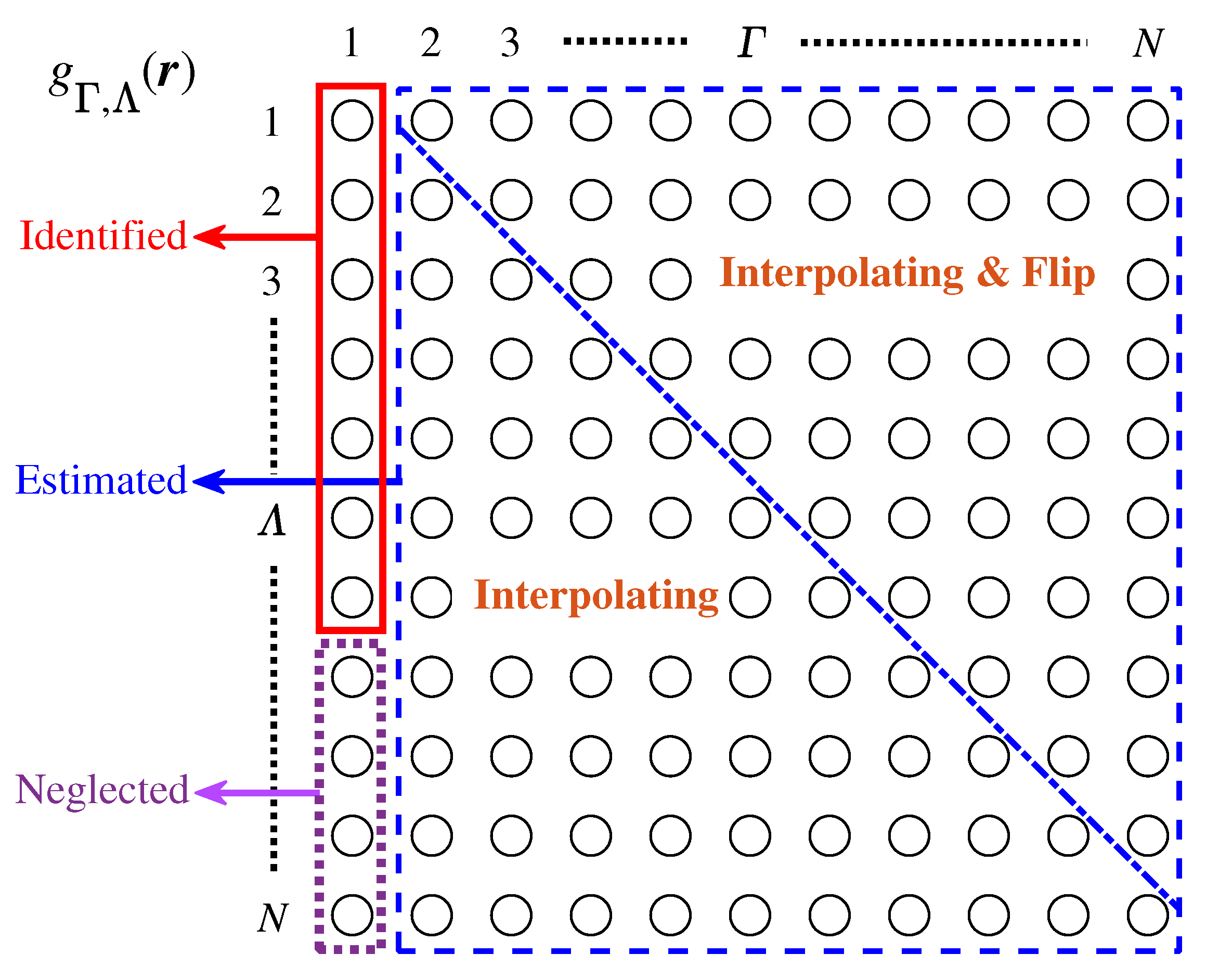
2.2. Low-Complexity Versatile Beamforming Method

We define the acoustic transfer function (ATF), which elucidates the correlation between the emission weight coefficient and the difference–frequency wave acoustic field:

$$p_d^{\left(\Gamma ,\Lambda \right)}\left(\mathbf{r}\right)=P_1^{\left(\Gamma \right)}{\left[P_2^{\left(\Lambda \right)}\right]}^{\ast }{g}_{\Gamma ,\Lambda }\left(\mathbf{r}\right).$$

(8)

Since high-frequency waves are no longer considered below, the acoustic field below refers to the difference–frequency wave acoustic field. Through the identification of the ATF and optimization of the transmit weight coefficients, a versatile beamforming approach can be achieved [19]. However, the number of ATFs in the literature is $N^2$, requiring complex identification. By identifying a small part of the ATF and estimating or neglecting the remainder, the complexity of the beamforming method can be significantly reduced.

According to the spatial relationships between different parameter arrays, the total acoustic field can be decomposed into three parts:

$$\begin{array}{c}{p}_d\left(\mathbf{r}\right)={\displaystyle \sum _{\Gamma =1}^N}\left[P_1^{\left(\Gamma \right)}{P_2^{\left(\Gamma \right)}}^{\ast }{g}_{\Gamma ,\Gamma }\left(\mathbf{r}\right)\right]+\hfill \\ {\displaystyle \sum _{\Gamma =1}^{N-1}}\left[P_1^{\left(\Gamma \right)}{\left(P_2^{\left(\Gamma +1\right)}\right)}^{\ast }{g}_{\Gamma ,\Gamma +1}\left(\mathbf{r}\right)\right]+{\displaystyle \sum _{\Gamma =1}^{N-2}}\left[P_1^{\left(\Gamma \right)}{\left(P_2^{\left(\Gamma +2\right)}\right)}^{\ast }{g}_{\Gamma ,\Gamma +2}\left(\mathbf{r}\right)\right]+\dots +\hfill \\ {\displaystyle \sum _{\Gamma =1}^{N-1}}\left[P_1^{\left(\Gamma +1\right)}{\left(P_2^{\left(\Gamma \right)}\right)}^{\ast }{g}_{\Gamma +2,\Gamma }\left(\mathbf{r}\right)\right]+{\displaystyle \sum _{\Gamma =1}^{N-2}}\left[P_1^{\left(\Gamma +2\right)}{\left(P_2^{\left(\Gamma \right)}\right)}^{\ast }{g}_{\Gamma +2,\Gamma }\left(\mathbf{r}\right)\right]+\dots .\hfill \end{array}$$

(9)

The first row corresponds to self SSS. The second row corresponds to the mutual SSS, where $\Gamma <\Lambda$. The third row corresponds to the mutual SSS, where $\Gamma >\Lambda$. For self SSS and mutual SSS under the condition of $\Gamma \le \Lambda$, the estimated ATF $g_{\Gamma ,\Lambda }$ is the coordinate translation of $g_{1,\Lambda -\Gamma +1}$ due to the same array formation with $\Lambda -\Gamma$. For mutual SSS under the condition of $\Gamma >\Lambda$, the estimated ATF $g_{\Gamma ,\Lambda }$ is the coordinate translation and 180° rotation of $g_{1,\Gamma -\Lambda +1}$ due to the symmetry of mutual SSS.

In the scenario of Figure 2, the ATFs can be estimated using the above conversion relationship. First, the condition of $\Gamma \le \Lambda$ is discussed. For the arrays forming $g_{\Gamma ,\Lambda }$ and $g_{1,\Lambda -\Gamma +1}$, the displacement between the two arrays in the x direction is $d_{\Gamma ,1}=d_{\Gamma }-d_1$, where the subscript represents the number of array elements. Therefore, the ATFs of $\Gamma \le \Lambda$ can be estimated as

$$\begin{array}{c}{\widehat{g}}_{\Gamma ,\Lambda }\left(x\right)=g_{1,\Lambda -\Gamma +1}\left[x-d_{\Gamma ,1}\right],\Gamma \le \Lambda .\hfill \end{array}$$

(10)

Secondly, the condition of $\Gamma >\Lambda$ is discussed. For the arrays forming $g_{\Gamma ,\Lambda }$ and $g_{1,\Gamma -\Lambda +1}$, the array formation is symmetrical along the x-axis. $g_{1,\Gamma -\Lambda +1}$ is mirror flipped along the x-axis; then, the relationship between flipped $g_{1,\Gamma -\Lambda +1}$ and $g_{\Gamma ,\Lambda }$ reduces to a coordinate translation transformation like Equation (10). The translational displacement from flipped $g_{1,\Gamma -\Lambda +1}$ to $g_{\Gamma ,\Lambda }$ is $\overline{d_{\Gamma ,1}}=d_{\Gamma }-\left(-d_1\right)=d_{\Gamma }+d_1.$, where superscript “$\overline{·}$” represents mirror flip. Therefore, the ATFs of $\Gamma >\Lambda$ can be estimated as

$$\begin{array}{c}{\widehat{g}}_{\Gamma ,\Lambda }\left(x\right)=g_{1,\Gamma -\Lambda +1}\left[-\left(x-\overline{d_{\Gamma ,1}}\right)\right],\Gamma >\Lambda .\hfill \end{array}$$

(11)

Although the acoustic field control positions are discretely arranged along the x-axis with a spacing $\Delta x$, $\widehat{g_{\Gamma ,\Lambda }}$ can be obtained by interpolation and flipping. Therefore, we can obtain the total ATFs($N^2$) by identifying $g_{1,1}\sim g_{1,N}$(N).

Futhermore, when the spacing of two parametric arrays is large, the influence of this part of mutual SSS on the total acoustic field is small. At this time, this part of the ATFs can be ignored. In order to quantitatively determine which ATFs can be ignored, here, we introduce sound pressure level error on the radiator axis as the threshold. The emission weight coefficient of each array element is set as the same, assuming that the spacing of MPAs is much smaller than the wavelength of difference–frequency waves. At this point, the sound pressure level error neglecting the ATFs $g_{1,Q+1}\sim g_{1,N}$ can be approximately expressed as

$$\begin{array}{c}\Delta \mathrm{SPL}\left(Q\right)=20\lg \left[{\displaystyle \frac{N\left|g_{1,1}\right|+{\displaystyle \sum _{q=2}^Q}2\left(N-q+1\right)\left|g_{1,q}\right|}{N\left|g_{1,1}\right|+{\displaystyle \sum _{q=2}^Q}2\left(N-q+1\right)\left|g_{1,q}\right|+\left(N-Q\right)\left(N-Q+1\right)\left|g_{1,Q}\right|}}\right],\hfill \end{array}$$

(12)

where $\left|g_{1,Q+1}\right|\sim \left|g_{1,N}\right|$ are approximated by $\left|g_{1,Q}\right|$.

Because $\left|g_{1,Q}\right|$ is inversely proportional to Q, $\Delta \mathrm{SPL}\left(Q\right)$ should converge with Q to the upper limit 0 dB. When the threshold related to the beamforming effect is determined, Q can be confirmed. $\left|g_{1,Q+1}\right|\sim \left|g_{1,N}\right|$ are always higher than $\left|g_{1,Q}\right|$; the real error will be slightly lower than the selected threshold, which is beneficial to the beamforming effect.

Figure 3 illustrates the schematic diagram of the simplification of beamforming complexity. The circle represents the ATF matrix. The red solid line corresponds to the part that needs to be identified, while the blue dashed line corresponds to the estimated part. Additionally, the blue dotted line distinguishes between the two types of SSS, $\Gamma \le \Lambda$ and $\Gamma >\Lambda$, and the ATFs are estimated using different formulas in Equations (10) and (11). The purple dotted line corresponds to the neglected part in $g_{1,\Lambda }$. Therefore, by estimating, the number of ATFs necessitating identification can be reduced from $N^2$ to N. By neglecting ATFs according to the threshold, the identified ATFs number can be further reduced from N to Q.

Finally, utilizing the ATF matrix obtained from Figure 3, the emission weight coefficient is optimized. Two distinct optimization objective functions are selected, corresponding to the absolute value and relative value, respectively.

$$\begin{array}{c}\underset{P_i^{\left(\Gamma \right)}}{\min }\left[{{\displaystyle \sum _{\mathbf{r}}}\left|p_d\left(\mathbf{r}\right)-\widehat{p_d}\left(\mathbf{r}\right)\right|}^2\right],\mathrm{func}\mathrm{I},\hfill \\ \underset{P_i^{\left(\Gamma \right)}}{\min }\left[{\displaystyle \sum _{\mathbf{r}}}\left|20\lg \left|p_d\left(\mathbf{r}\right)/\phantom{p_d\left(\mathbf{r}\right)\widehat{p_d}\left(\mathbf{r}\right)}\widehat{p_d}\left(\mathbf{r}\right)\right|\right|\right],\mathrm{func}\mathrm{II}.\hfill \end{array}$$

(13)

In addition, the proposed beamforming method is also not limited by far-field conditions because the method does not involve any far-field approximation. In the case of small-aperture unsaturated acoustic excitation, absorption range dominates the effective array length of MPAs, which are inversely proportional to the sound absorption coefficient of high-frequency waves [23]. Setting the sound absorption coefficients of the two high-frequency waves and the difference–frequency wave as ${\alpha }_1,{\alpha }_2,{\alpha }_d$, the effective array length of MPAs can be expressed as

$$L_{\alpha }=1/\phantom{1\left({\alpha }_1+{\alpha }_2-{\alpha }_d\right)}\left({\alpha }_1+{\alpha }_2-{\alpha }_d\right)$$

(14)

The difference–frequency wave follows inverse-law attenuation over $L_{\alpha }$, that is, the far field of MPAs. In the far field, nonlinear interaction of high-frequency waves is completed, and a high directional acoustic beam is fully formed. However, $L_{\alpha }$ is generally large, so the target to be detected or communicated is not always located in the far field. For example, the inverse-law far field of a parametric array loudspeaker is more than 10 m in most cases [24], while the application scenario is often bounded spaces such as rooms or cars. For another example, the effective array length of a parametric sub-bottom profiler is over 100 m according to the seawater sound absorption coefficients, so the seabed is unlikely to satisfy the far field condition in shallow sea surveys [25]. Under the non-far field scenarios, the proposed beamforming method is also available.

3. Results and Discussions

3.1. Setup of the Numerical Model

We set $a_x=0.75\mathrm{cm},a_y=5\mathrm{cm}$, the number of MPAs $N=11$, and the spacing $d=2\mathrm{cm}$. The medium for sound propagation was freshwater, the parameters of which were ${\rho }_0=1000\mathrm{kg}/\phantom{\mathrm{kg}{\mathrm{m}}^3}{\mathrm{m}}^3,c_0=1500\mathrm{m}/\phantom{\mathrm{m}\mathrm{s}}\mathrm{s},\beta =3.5$, and the sound absorption coefficient was obtained from the empirical formula in freshwater. We set high frequency $\left(f_1+f_2\right)/\phantom{\left(f_1+f_2\right)2}2=40\mathrm{kHz}$ and difference–frequency $f_d=4\mathrm{kHz}$. As for the acoustic field control positions, the parameters were $z_0=10\mathrm{m},\Delta x=0.2\mathrm{m}$. Under the condition that the equivalent sound pressure on the radiant surface was set to $P_i^{\left(\Gamma \right)}={10}^5\mathrm{Pa}$, the acoustic field of MPAs was modeled by Equations (4) and (7).

The acquisition of Gaussian expansion coefficients in Equations (6) and (7) is a multivariable nonlinear optimization problem. The objective function [21] is similar to function I in Equation (13), corresponding to the root mean square error (RMSE) of exact distribution and Gaussian expansion distribution. The normalized coordinate $\tilde{r}$ to construct the optimization function ranges from 0 to 5. The optimization algorithm employs the interior-point method. The dimensionless and normalized vibration velocity of piston source exhibits a step function distribution, which can be well fitted by 10 Gaussian functions ($M=10$), as shown in Figure 4. Herein, the iteration stop criterion was $\mathrm{RMSE}\le 0.04$. The Gaussian expansion coefficients of these Gaussian functions are presented in

Table 1. Gaussian expansion coefficients of the dimensionless and normalized vibration velocity of the piston source.

m	${\mathit{A}}_{\mathit{m}}$	${\mathit{B}}_{\mathit{m}}$
1	− 8.636 − 11.994j	2.471 + 9.361j
2	−0.701 + 5.069j	3.273 + 2.222j
3	0.387 + 0.600j	2.014 − 6.381j
4	−0.932 − 4.006j	3.104 − 2.246j
5	3.674 + 8.678j	3.221 − 11.464j
6	2.258 + 7.653j	2.200 + 9.692j
7	−0.115 + 0.070j	1.150 − 17.475j
8	8.287 + 3.086j	2.946 + 8.496j
9	−0.107 + 0.089j	1.120 + 16.248j
10	−3.135 − 9.191j	3.289 − 11.143j

. Herein, “j” represents the unit imaginary number.

The acoustic field calculation model described in Section 2.1 of this paper employs the conventional Gaussian beam expansion (GBE) within the paraxial approximation, while Equation (10) in reference [10] is founded on the non-paraxial Gaussian beam expansion under the approximation (NGBE). The two models were compared with the exact solution calculated by the triple integral Equation (2) to validate the effectiveness. Figure 5 shows the acoustic field distribution of multiple parametric arrays. With a field point X-coordinate range of $\pm 4\mathrm{m}$, corresponding to the angle of $\pm 21.8^{\circ }$, sound pressure level (SPL) calculated by GBE and NGBE was generally consistent with the exact solution. RMSE of SPL was obtained within the angle range to quantitatively compare GBE and NGBE. SPL RMSE for GBE was 0.28 dB, lower than the NGBE value of 0.56 dB. The maximum calculation error of GBE did not exceed 0.5 dB within $\pm {20}^{\circ }$, which could be considered an effective angle range of GBE modeling in this radiator scenario. Due to the form of paraxial approximation, the calculation accuracy of the half-power beamwidth of GBE was wider than NGBE under non-paraxial approximation: beamwidth calculated by GBE was ${10}^{\circ }$, which was consistent with the exact solution, while the value of NGBE was $9^{\circ }$. Therefore, the numerical model was set up based on GBE, and ATF estimation and beamforming were conducted through the acoustic field calculated by the model.

In addition, according to Rayleigh integral, equivalent sound pressure on a radiant surface with a value of ${10}^5\mathrm{Pa}$ corresponds to a 210 dB sound source level of high-frequency waves. It can be observed from Figure 5 that the sound source level of the difference–frequency wave was several orders of magnitude lower than that of the high-frequency wave. Low conversion efficiency [26] is indeed an inherent shortcoming of parametric array systems. However, the unique application of the parametric array system in low-frequency small-aperture high-resolution acoustic excitation cannot reasonably be replaced by other types of sound sources. In practical applications, what we are applying is the difference–frequency wave in MPAs. The required difference–frequency acoustic signal can be easily separated through time–frequency analysis.

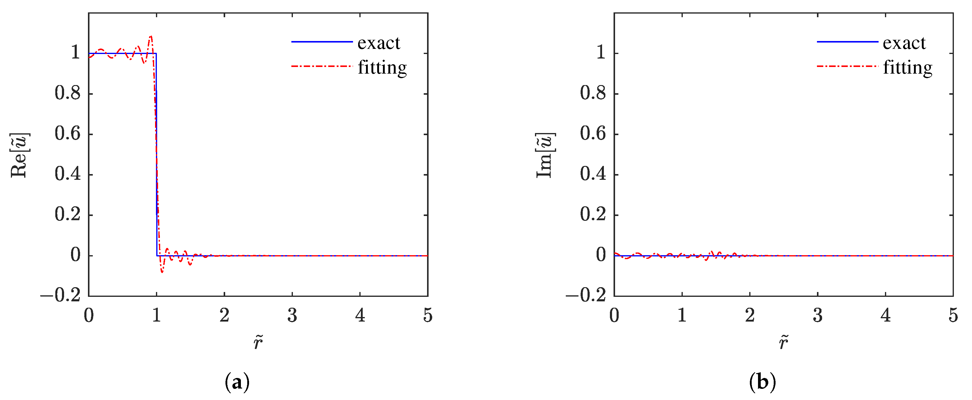
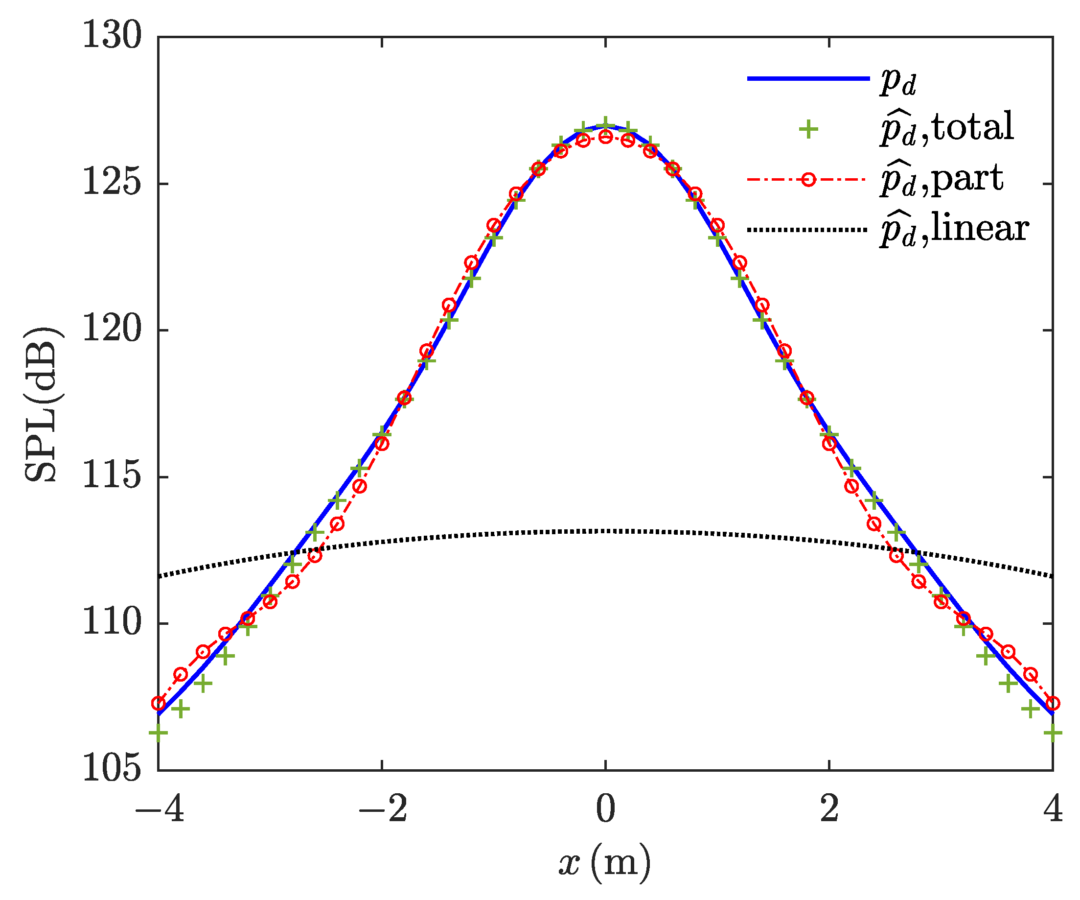
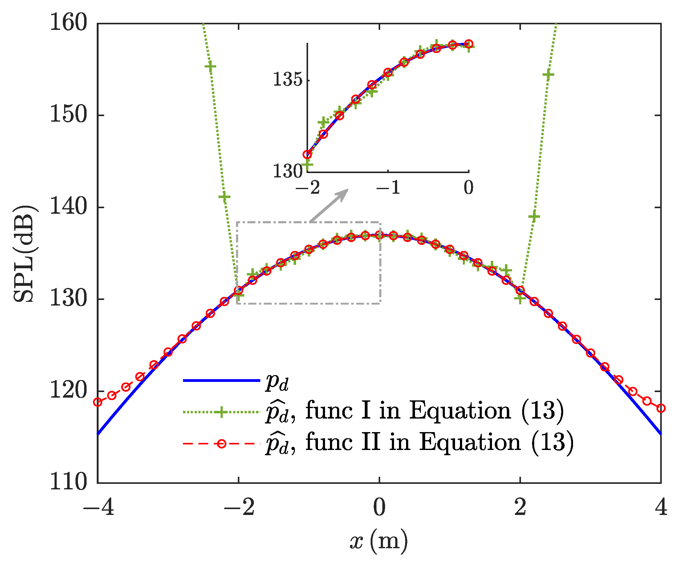
3.2. Estimation of Acoustic Transfer Function

Three typical components in Equation (9) were selected to validate the effectiveness of ATF estimation, that is, self SSS, mutual SSS where $\Gamma <\Lambda$, and mutual SSS where $\Gamma >\Lambda$. ${\widehat{g}}_{7,7}$ corresponds to the self SSS, which could be estimated from ${\widehat{g}}_{1,1}$ based on Equation (10). ${\widehat{g}}_{7,8}$ corresponds the mutual SSS where $\Gamma <\Lambda$, which can be estimated from ${\widehat{g}}_{1,2}$ based on Equation (10). ${\widehat{g}}_{9,7}$ corresponds to the mutual SSS where $\Gamma >\Lambda$, which can be estimated from ${\widehat{g}}_{1,3}$ based on Equation (11). The estimation accuracy was reflected by the acoustic field of $p_d^{\left(\Gamma ,\Lambda \right)}$, as shown in Figure 6. It can be seen that the exact value $p_d^{\left(\Gamma ,\Lambda \right)}$ and the estimated value ${\widehat{p}}_d^{\left(\Gamma ,\Lambda \right)}$ were basically consistent regardless of amplitude or phase.

Substituting the estimated ATF $\widehat{g_{\Gamma ,\Lambda }}$ into Equation (8), the normalized sound pressure level at the radiator axis could be obtained, expressed as $\widetilde{\mathrm{SPL}}$.

Figure 7 shows the influence of each component on the total acoustic field. Figure 7a presents the normalization sound pressure level of ${\widehat{p}}_d^{\left(\Gamma ,\Lambda \right)}$ on the radiator axis. The blue dashed line corresponds to the ATF considering the total. The purple dotted line corresponds to the ATF only considering the self SSS, that is, the linear superposition of the acoustic field generated by each parameter array. Obviously, $\widetilde{\mathrm{SPL}}$ was highest in the linear part. The red dotted line separates the area with low SPL, where the two parametric arrays participating in the interaction were far apart. This part of the ATF could be considered neglected when estimating the total acoustic field. The neglected part is presented in Figure 7b, which is a convergence curve obtained by Equation (12). The threshold value was set as −1 dB. It can be seen that the identified ATFs number $Q=7$ reached the convergence condition. $Q=7$ meant that ATFs within $\left|\Gamma -\Lambda \right|\ge 7$ could be neglected, which corresponds to the area outside two red dashed lines. Thus, the identified ATFs number could be further reduced from N to 7. In practical application, we start the identification from $g_{1,7}$ and end at $g_{1,7}$. Further consideration of $Q=8\sim 11$ in Figure 7b is to reflect the convergence of $\Delta \mathrm{SPL}\left(Q\right)$.

Considering different parts of ATFs, an acoustic field reconstructed from different parts of estimated ATFs was compared with the exact SPL of $p_d$, as shown in Figure 8. When the total of the ATFs were considered, the identified and estimated ATFs could basically reconstruct the exact acoustic field, which reflected the high accuracy of the estimation. This is hereafter referred to as a total scheme. When the part of $\left|\Gamma -\Lambda \right|\ge 7$ are neglected, the estimated SPL has a slight error from the exact, but it remains within an acceptable range. This phenomenon is due to the neglected part in Figure 7. Hereinafter referred to as part scheme.

When only the linear part in Figure 7 was considered, the estimated SPL on the radiator axis was much lower than the exact. This was because the magnitude of mutual SSS was the same as self SSS under the parameters of this study, as shown in Figure 6, rendering the mutual SSS non-negligible. This is hereafter referred to as the linear scheme. Reconstructed SPL RMSE of total scheme and part scheme were 0.29 dB and 0.52 dB, far less than the linear scheme’s 7.39 dB. The high reconstruction error of 7.39 dB meant that the linear scheme was not suitable for estimating the acoustic field of MPAs. Thus, the effectiveness of the ATF estimation was validated, while demonstrating the feasibility of the part scheme and linear scheme to estimate the total acoustic field.

This study validated the effectiveness of the ATF estimation and demonstrated the feasibility of the part scheme for estimating the total acoustic field. On this basis, the beamforming for MPAs was conducted and its effect is discussed.

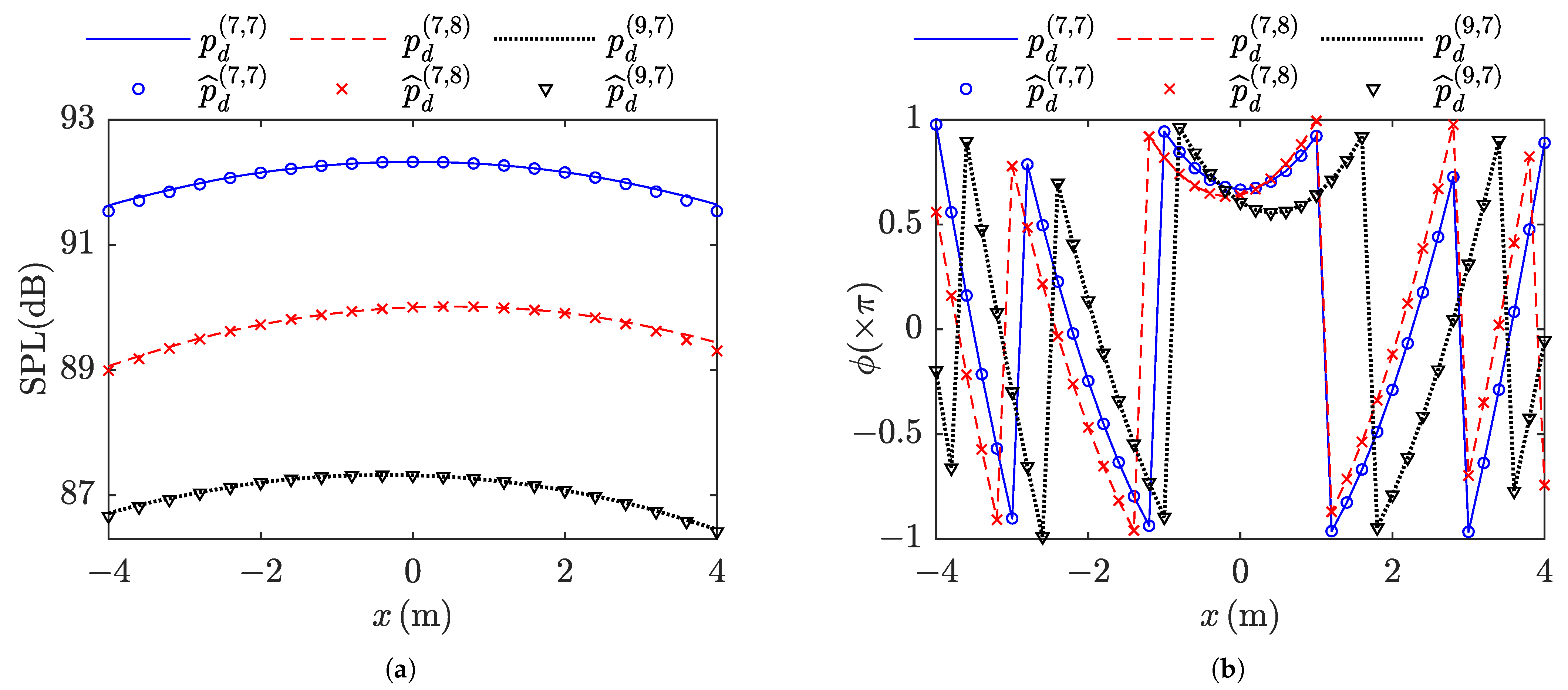
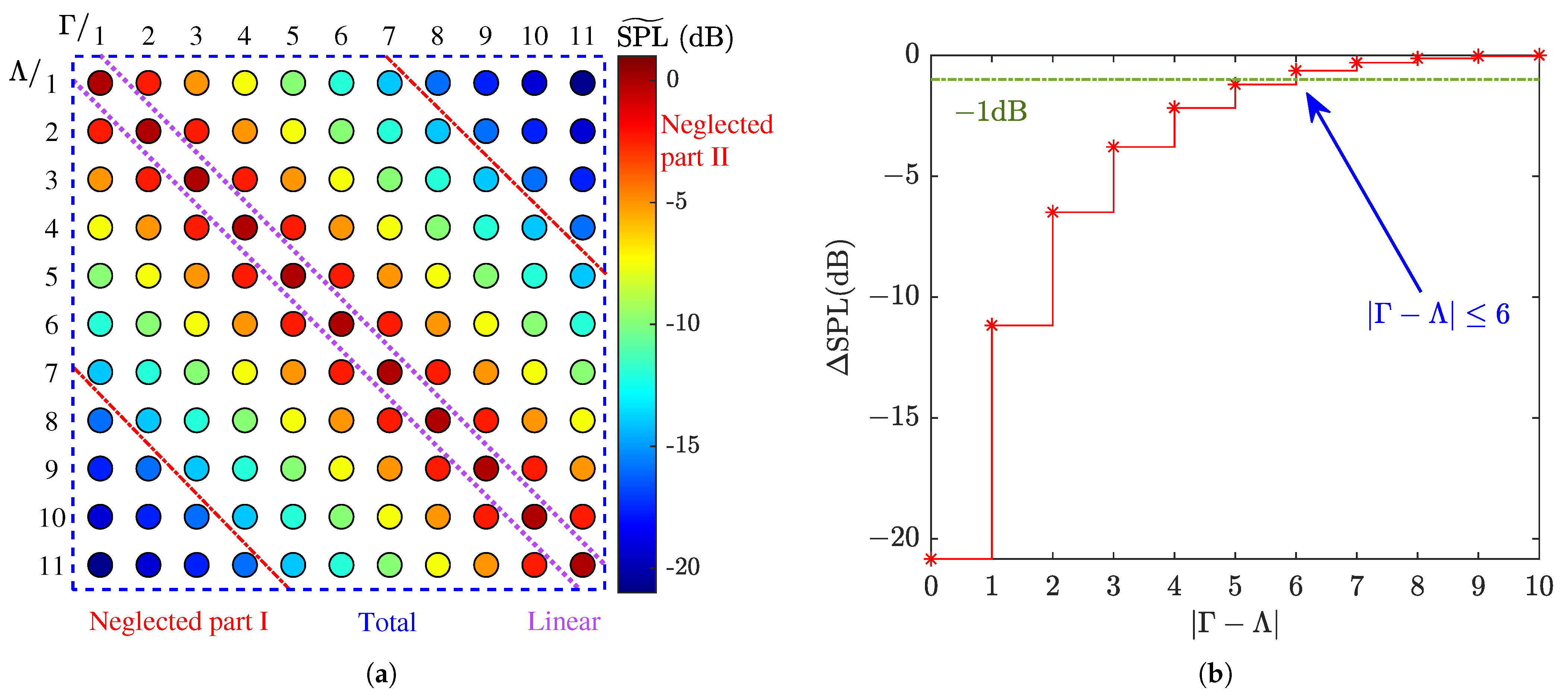
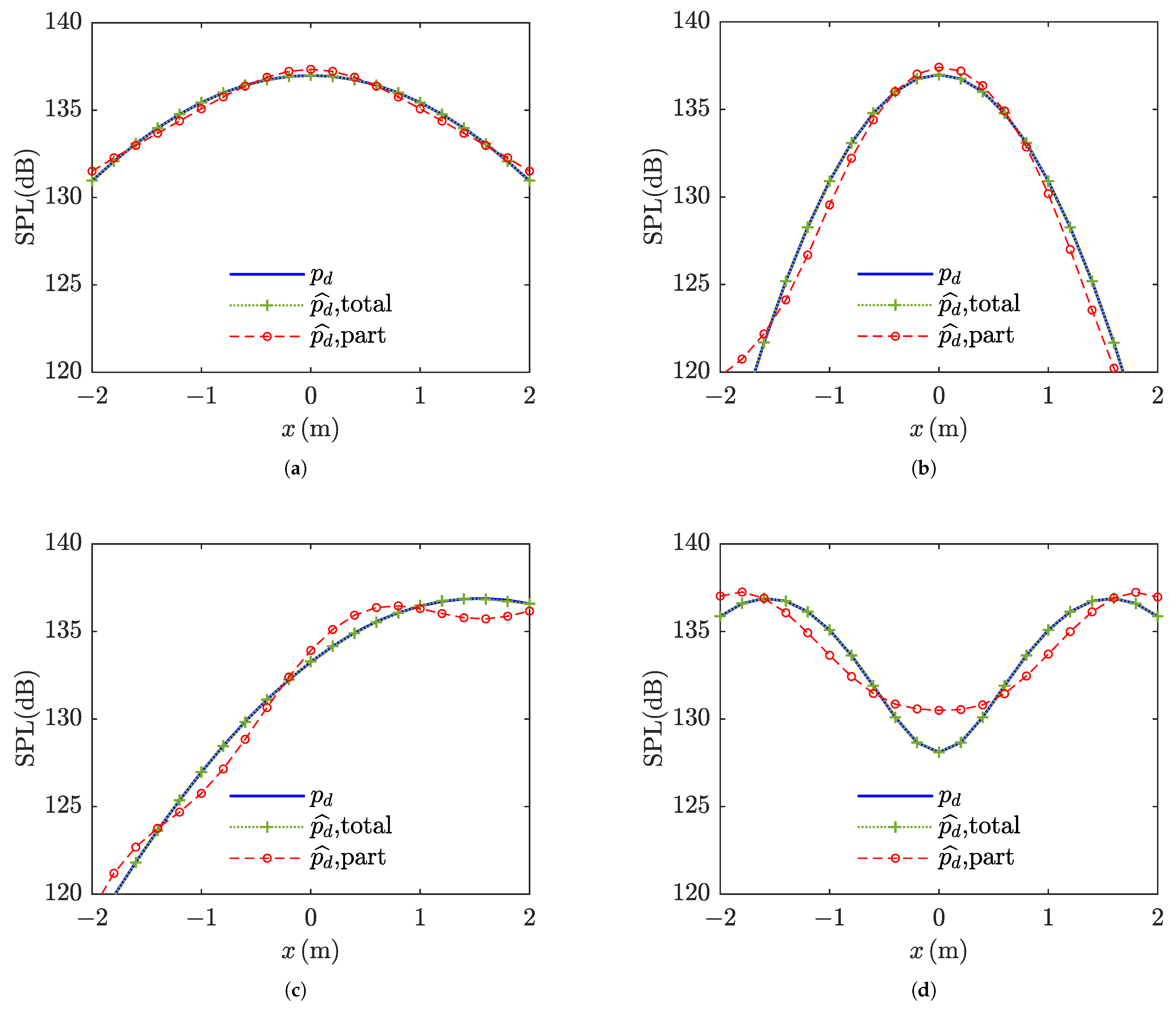
3.3. Beamforming Effect of Multiple Parametric Arrays

The desired acoustic field was constructed using Gaussian beam as follows:

$$p_d\left(\mathbf{r}\right)={\displaystyle \frac{P_d}{r}}\sum _{l=1}^L\exp \left\{-{\left({\displaystyle \frac{k_d}{2}}{A}_x\right)}^2·{\left[{\displaystyle \frac{x}{r}}-\sin \left({\phi }_x^{\left(l\right)}\right)\right]}^2+\mathrm{j}{k}_{d}r\right\}$$

(15)

where the emitted complex sound pressure $P_d=100\mathrm{Pa}$, $A_x$ denotes the size of radiating surface that could control the half-power beamwidth, and ${\phi }_x^{\left(l\right)}$ denotes the steering angle of the radiator axis. The sum operator was utilized to generate the dual beam.

On the condition that $A_x=0.5\mathrm{m},{\phi }_x^{\left(l\right)}=0^{\circ },L=1$, and the acoustic field control positions were arranged at −2 m∼2 m. Figure 9 shows the beamforming effect based on different optimization objective functions. It can be observed that SPL of $\widehat{p_d}$ based on function I in Equation (13) was much higher than $p_d$ outside the beamforming region, while the SPL error of $\widehat{p_d}$ based on function II in Equation (13) was far less. Compared with function II, function I required not only consistent sound pressure level but also consistent phase. In the absence of constraints, function I tended to form high SPL outside the beamforming region. Within the beamforming region, the SPL error of $\widehat{p_d}$ based on function I was also higher than that of function II. This was because the desired acoustic field distribution was not the step function, the same as the vibration velocity in Figure 4, leading to the error in low SPL position. On the contrary, function II could be considered as the mean absolute error of SPL. Thus, function II presented a better beamforming effect of SPL in Figure 9. In cases where a uniform phase was unnecessary, function II was employed based on relative values for beamforming.

Considering different parts of ATFs, the beamforming effect is shown in Figure 10. The linear scheme only needed to identify 1 ATF, but formed much higher SPL than the desired acoustic field. Although mutual SSS was weaker than self SSS, mutual SSS had N times the number of self SSS and was also an important component of the acoustic field structure in MPAs, as shown in Figure 7a. By optimizing the emission weight coefficient, the linear scheme enabled self SSS to form the desired beam. However, all mutual SSS were also superimposed on this desired beam, resulting in the overtop SPL of the linear scheme. The total scheme and the part scheme needed to identify 11 and 7 ATFs separately. Beamforming SPL RMSE of the total scheme and part scheme were 0.01 dB and 0.30 dB, far less than the linear scheme’s 29.54 dB. The acoustic field formed by the total and part schemes was consistent with the desired acoustic field, which reflected the effectiveness of the low-complexity of the beamforming method.

Various beam patterns were formed using Equation (15) to access the versatility of the beamforming method in this paper. Figure 11 shows the beamforming effects for different beam patterns. The parameter of subgraph (a) was $A_x=0.5\mathrm{m},{\phi }_x^{\left(l\right)}=0^{\circ },L=1$, which formed beams with a wider half-power beamwidth of $15.9^{\circ }$ compared to the $9.9^{\circ }$ in Figure 5. The parameter of subgraph (b) was $A_x=1\mathrm{m},{\phi }_x^{\left(l\right)}=0^{\circ },L=1$, which formed beams with a narrower half-power beamwidth of $8.1^{\circ }$. The parameter of subgraph (c) was $A_x=0.5\mathrm{m},{\phi }_x^{\left(l\right)}=9^{\circ },L=1$, which formed steered beams. The parameter of subgraph (d) was $A_x=1\mathrm{m},{\phi }_x^{\left(l\right)}=9^{\circ },L=2$, which formed notched beams. The acoustic field formed by the total scheme closely matched the desired acoustic field across different beam patterns. Although the part scheme obtained higher SPL error owing to the neglected estimation part of ATFs, the beamforming patterns of different types could be clearly observed. For further quantitative analysis, SPL RMSE of four beam types obtained by the total scheme and part scheme are compared in

Table 2. SPL RMSE of four beam types obtained by the total scheme and part scheme.

Beam Type	SPL RMSE of Total Scheme	SPL RMSE of Part Scheme
wide beam	0.01	0.30
narrow beam	0.01	1.83
steered beam	0.02	0.87
notched beam	0.01	1.16

. SPL RMSE of the total scheme was all less than 0.01 dB, while SPL RMSE of the part scheme was 1dB averagely. SPL RMSE of the narrow beam obtained by the part scheme reached the maximum value of 1.83 dB. We speculate that the high RMSE might have been due to the necessity of ATFs with high $\left|\Gamma -\Lambda \right|$ while maintaining high directivity. Overall, for this MPA system, the total scheme had an excellent beamforming effect, with SPL RMSE less than 0.1 dB, while 11 ATFs needed to be identified, and the part scheme only needed to identify 7 ATFs with a cost of a 1 dB average reduction of the beamforming effect. The number of identified ATFs and beamforming effect should be balanced according to practical application scenarios.

In summary, the proposed beamforming method for MPAs is a low-complexity and versatile method that could form various beam patterns and reduce the number of identified ATFs from 121 to 11 in the total scheme or 7 in the part scheme. The high control flexibility allows the MPA system to detect or communicate with variable targets, such as with seafloor sediment mapping and directional underwater communication. Although the acoustic propagation medium in this study was freshwater, the generation mechanism of the MPA acoustic field remains consistent across different media. Therefore, the proposed method is equally applicable to parametric array loudspeakers in a free field. However, the proposed beamforming method has the following problems. First, the conversion efficiency from high-frequency wave to difference–frequency wave is low, which is an inherent cost of the parametric array system. Secondly, the proposed beamforming method has only been theoretically validated in a simulation environment, lacking experimental research. Beamforming in this study was conducted in a free field, which is expected to expand to a non-free field. Similar to receive array beamforming [27], transmit beamforming also faces the challenge of interface interference control. In the future, we will conduct an experimental study and expand the proposed beamforming method to an ocean waveguide.

4. Conclusions

This paper proposed a low-complexity versatile beamforming method for multiple parametric arrays. First, the acoustic field structure of MPAs was examined, encompassing self SSS and mutual SSS. The acoustic field of each SSS could be modeled using GBE under the paraxial approximation. Secondly, we derived the transitive relationship between acoustic transfer functions. For N parametric arrays, the number of identified ATFs could be reduced from N² to N, estimating the remaining ATFs by interpolation and flipping. By setting a specified convergence threshold to neglect the less affected part, further reductions below N could be achieved. On the basis of the obtained ATF matrix, the emission weight coefficient was then optimized to form the desired beam pattern. Subsequently, a numerical model was set up using GBE and validated against the exact solution. The ATF estimation and beamforming effect were discussed through the acoustic field calculated by the model. Comparing with the exact and estimated ATF, the high estimated accuracy was ensured. Under the condition of $N=11$, the acoustic field could be reconstructed by 11 identified ATFs considering the total ATFs or 7 identified ATFs neglecting the less affected part. The linear scheme only considered the linear part of ATFs, which led to substantial error in the estimated total acoustic field, resulting in a notably poor beamforming effect. Finally, the beamforming effects of MPAs were examined across four beam patterns. The total scheme reduced the number of identified ATFs from 121 to 11, precisely forming each desired acoustic field with a root mean square error of SPL less than 0.1 dB. The part scheme could further reduce the number of identified ATFs to 7 with a cost of a 1 dB average reduction of the beamforming effect. Despite a slight SPL error in the part scheme owing to the neglected part of ATF estimation, the beamforming patterns of different types remained clearly observable. Therefore, the proposed beamforming method’s low-complexity and versatility were verified, which provides a highly feasible solution for acoustic field control.

References

1. Cai, Y.; Wu, M.; Yang, J. Sound reproduction in personal audio systems using the least-squares approach with acoustic contrast control constraint. J. Acoust. Soc. Am. 2014, 135, 734–741. [Google Scholar] [CrossRef]
2. Demi, L.; Verweij, M.D.; van Dongen, K.W.A. Parallel Transmit Beamforming Using Orthogonal Frequency Division Multiplexing Applied to Harmonic Imaging—A Feasibility Study. IEEE Trans. Ultrason. Ferroelectr. Freq. Control 2012, 59, 2439–2447. [Google Scholar] [CrossRef]
3. Sharaga, N.; Tabrikian, J.; Messer, H. Optimal Cognitive Beamforming for Target Tracking in MIMO Radar/Sonar. IEEE J. Sel. Top. Signal Process. 2015, 9, 1440–1450. [Google Scholar] [CrossRef]
4. Cuji, D.A.; Stojanovic, M. Transmit Beamforming for Underwater Acoustic OFDM Systems. IEEE J. Ocean. Eng. 2024, 49, 145–162. [Google Scholar] [CrossRef]
5. Westervelt, P.J. Parametric Acoustic Array. J. Acoust. Soc. Am. 1963, 35, 535–537. [Google Scholar] [CrossRef]
6. Gan, W.S.; Yang, J.; Kamakura, T. A review of parametric acoustic array in air. Appl. Acoust. 2012, 73, 1211–1219. [Google Scholar] [CrossRef]
7. Zhou, H.; Huang, S.H.; Li, W. Parametric Acoustic Array and Its Application in Underwater Acoustic Engineering. Sensors 2020, 20, 2148. [Google Scholar] [CrossRef]
8. Geng, Y.; Nakayama, M.; Nishiura, T. Narrow-edged beamforming based on individual phase inversion in amplitude-modulated wave for parametric array loudspeaker. Appl. Acoust. 2022, 200, 109060. [Google Scholar] [CrossRef]
9. Jiménez, N.; Ealo, J.; Muelas-Hurtado, R.D.; Duclos, A.; Romero-García, V. A helicoidal parametric antenna for subwavelength vortex generation. Proc. Mtgs. Acoust. 2022, 48, 045001. [Google Scholar]
10. Zhu, Y.; Ma, W.; Kuang, Z.; Wu, M.; Yang, J. Optimal audio beam pattern synthesis for an enhanced parametric array loudspeaker. J. Acoust. Soc. Am. 2023, 154, 3210–3222. [Google Scholar] [CrossRef]
11. Zhu, Y.; Zhang, Y.; Fan, F.; Ma, W.; Qin, L.; Kuang, Z.; Wu, M.; Yang, J. An enhanced beamsteering algorithm based on MVDR for a multi-channel parametric array loudspeaker array. J. Sound Vib. 2025, 595, 118768. [Google Scholar] [CrossRef]
12. Kelly, M.; McKinley, M.; Liu, G.; Shi, C. Evaluation of inner product-based demultiplexing of vortex-based underwater acoustic communications signals in realistic environments. J. Acoust. Soc. Am. 2024, 156, 3112–3117. [Google Scholar] [CrossRef]
13. Wang, C.; Zhu, G.; Tang, S.; Yin, J.; Guo, L.; Sheng, X.; Li, M. Directional bionic underwater communication method using a parametric acoustic array and recursive filtering. Appl. Acoust. 2022, 191, 108665. [Google Scholar] [CrossRef]
14. Yang, J.; Gan, W.S.; Tan, K.S.; Er, M.H. Acoustic beamforming of a parametric speaker comprising ultrasonic transducers. Sens. Actuators A Phys. 2005, 125, 91–99. [Google Scholar] [CrossRef]
15. Zhong, J.; Zou, H.; Lu, J.; Zhang, D. A modified convolution model for calculating the far field directivity of a parametric array loudspeaker. J. Acoust. Soc. Am. 2023, 153, 1439–1451. [Google Scholar] [CrossRef]
16. Tang, K.; Wang, Y.; Wang, S.; Gao, D.; Li, H.; Liang, X.; Sebbah, P.; Li, Y.; Zhang, J.; Shi, J. Hyperuniform Disordered Parametric Loudspeaker Array. Phys. Rev. Appl. 2023, 19, 054035. [Google Scholar] [CrossRef]
17. Skinner, E.; Groves, M.; Hinders, M.K. Demonstration of a length limited parametric array. Appl. Acoust. 2019, 148, 423–433. [Google Scholar] [CrossRef]
18. Nomura, H.; Nakagawa, T. Distortion reduction of length-limited sound beam generated by parametric acoustic array. Appl. Acoust. 2025, 230, 110425. [Google Scholar] [CrossRef]
19. Zhu, Y.; Qin, L.; Ma, W.; Fan, F.; Wu, M.; Kuang, Z.; Yang, J. A nonlinear sound field control method for a multi-channel parametric array loudspeaker array. J. Acoust. Soc. Am. 2025, 157, 962–975. [Google Scholar] [CrossRef]
20. Cervenka, M.; Li, W.; Huang, S.H. Non-paraxial model for a parametric acoustic array. J. Acoust. Soc. Am. 2013, 134, 933–938. [Google Scholar] [CrossRef]
21. Červenka, M.; Bednařík, M.; Koníček, P. Numerical simulation of parametric field patterns of ultrasonic transducer arrays. In Proceedings of the 2009 IEEE International Ultrasonics Symposium, Rome, Italy, 20–23 September 2009. [Google Scholar]
22. Xu, L.; Zhang, H.; Zhang, M. Training a Deep Operator Network as a Surrogate Solver for Two-Dimensional Parabolic-Equation Models. J. Acoust. Soc. Am. 2023, 154, 3276–3284. [Google Scholar] [CrossRef] [PubMed]
23. Kopp, L.; Cano, D.; Dubois, E.; Wang, L.; Smith, B.; Coates, R.F. Potential performance of parametric communications. IEEE J. Oceanic Eng. 2000, 25, 282–295. [Google Scholar] [CrossRef]
24. Zhong, J.X.; Kirby, R.; Qiu, X.J. The near field, Westervelt far field, and inverse-law far field of the audio sound generated by parametric array loudspeakers. J. Acoust. Soc. Am. 2021, 143, 1524–1535. [Google Scholar] [CrossRef] [PubMed]
25. Zhou, H.Y.; Li, W.; Huang, S.H. Signal Processing Algorithm and System Realization of Broadband Parametric Array Sub-Bottom Profiler. IEEE Sensors J. 2022, 22, 17090–17102. [Google Scholar] [CrossRef]
26. Li, M.; Zhong, J.; Jing, Y.; Lu, J. A note on the audio sound power generated by a parametric array loudspeaker. J. Acoust. Soc. Am. 2023, 154, 3899–3905. [Google Scholar] [CrossRef]
27. Chen, H.; Zhu, Z.; Yang, D. Conventional Beamforming Algorithm Based on Polarization Filtering for an Acoustic Vector-Sensor Linear Array Mounted Near a Baffle. IEEE J. Ocean. Eng. 2024, 49, 1127–1139. [Google Scholar] [CrossRef]
Figure 1. Acoustic field structure of multiple parametric arrays. The total acoustic field consists of two types of scattering of sound by sound. p d Γ , Γ , p d Λ , Λ is generated by an emission transducer through self-interaction, while p d Γ , Λ , p d Λ , Γ is generated by different emission transducers through mutual interaction.
Acoustics 07 00037 g001
Figure 2. Schematic of multiple parametric arrays in beamforming scenarios. Multiple parameter arrays are uniformly arranged on the x-axis. The acoustic field control positions are located on the O x z plane, uniformly arranged along the x-direction at a distance of z 0 from the geometric center of the array.
Acoustics 07 00037 g002
Figure 3. Schematic diagram of reducing the complexity of beamforming. Beamforming requires N 2 acoustic transfer functions g Γ , Λ , represented by the circles. By interpolation and flipping, ATFs within the blue dashed line can be estimated. By comparing the intensity of ATFs, ATFs within the purple dotted line can be neglected, that is, there is no need to identify ATFs with Γ Λ higher than a certain threshold. At this time, the number of ATFs that need to be identified can be reduced from N 2 to, at most, N, represented by the red solid line.
Acoustics 07 00037 g003
Figure 4. Gaussian function fitting of vibration velocity: (a) real part; (b) imaginary part. The exact vibration velocity of piston source exhibited a step function distribution, represented by the blue solid line. The fitting vibration velocity by 10 Gaussian functions corresponds to the red dotted line.
Acoustics 07 00037 g004
Figure 5. Acoustic field distribution of multiple parametric arrays. The red dashed line, green dotted line, and blue solid line correspond to the acoustic field modeled by GBE, NGBE, and the exact solution in sequence. In order to clearly reflect the differences among the three, the half power beamwidth is locally enlarged.
Acoustics 07 00037 g005
Figure 6. Estimated acoustic field of p d Γ , Λ : (a) amplitude; (b) phase. Lines correspond to the exact value p d Γ , Λ of three types, while markers correspond to the estimated value p ^ d Γ , Λ .
Acoustics 07 00037 g006
Figure 7. Influence of each component on the total acoustic field. (a) Normalization sound pressure level of p ^ d Γ , Λ on the radiator axis. (b) Convergence curve of the neglected part selection. Color-filled circles represent each component of the total acoustic field, wherein the color corresponds to the normalized sound pressure level of p ^ d Γ , Λ . The red dashed line separates the neglected parts and the reserved part, corresponding to the part scheme. The purple dotted line separates self and mutual scattering of sound by sound, corresponding to the linear scheme. The red ladder line reflects the identified ATF number Q on the sound pressure level error on the radiator axis. The green dashed line represents convergence threshold.
Acoustics 07 00037 g007
Figure 8. Acoustic field reconstruction from different parts of estimated ATFs. The blue solid line corresponds to the exact sound pressure level of p d . The green “+”, red dashed line, and black dotted line correspond to the estimated values by total scheme, part scheme, and linear scheme in sequence.
Acoustics 07 00037 g008
Figure 9. Beamforming effect based on different optimization objective functions. The blue solid line corresponds to the exact sound pressure level of p d . The green dotted line and red dashed line correspond to the estimated values by func I and fun II in Equation (13), respectively.
Acoustics 07 00037 g009
Figure 10. Beamforming effect based on different parts of ATFs. The blue solid line corresponds to the exact sound pressure level of p d . The green dotted line, red dashed line, and yellow solid line represent the beamforming effect of the total scheme, part scheme, and linear scheme, respectively.
Acoustics 07 00037 g010
Figure 11. Beamforming effects for different beam patterns: (a) beam with wider half-power beamwidth; (b) beam with narrower half-power beamwidth; (c) steered beam; (d) notched beam. The blue solid line corresponds to the exact sound pressure level of p d . The green dotted line and red dashed line represent the beamforming effect of the total scheme and part scheme, respectively.
Acoustics 07 00037 g011