Open-Set Recognition of Environmental Sound Based on KDE-GAN and Attractor–Reciprocal Point Learning

Abstract

While open-set recognition algorithms have been extensively explored in computer vision, their application to environmental sound analysis remains understudied. To address this gap, this study investigates how to effectively recognize unknown sound categories in real-world environments by proposing a novel Kernel Density Estimation-based Generative Adversarial Network (KDE-GAN) for data augmentation combined with Attractor–Reciprocal Point Learning for open-set classification. Specifically, our approach addresses three key challenges: (1) How to generate boundary-aware synthetic samples for robust open-set training: A closed-set classifier’s pre-logit layer outputs are fed into the KDE-GAN, which synthesizes samples mapped to the logit layer using the classifier’s original weights. Kernel Density Estimation then enforces Density Loss and Offset Loss to ensure these samples align with class boundaries. (2) How to optimize feature space organization: The closed-set classifier is constrained by an Attractor–Reciprocal Point joint loss, maintaining intra-class compactness while pushing unknown samples toward low-density regions. (3) How to evaluate performance in highly open scenarios: We validate the method using UrbanSound8K, AudioEventDataset, and TUT Acoustic Scenes 2017 as closed sets, with ESC-50 categories as open-set samples, achieving AUROC/OSCR scores of 0.9251/0.8743, 0.7921/0.7135, and 0.8209/0.6262, respectively. The findings demonstrate the potential of this framework to enhance environmental sound monitoring systems, particularly in applications requiring adaptability to unseen acoustic events (e.g., urban noise surveillance or wildlife monitoring).

1. Introduction

Acoustic target recognition is a well-explored field with applications in human voice recognition, environmental audio classification, and music categorization. The goal is to establish a mapping from audio samples to their corresponding labels, which can be broadly categorized into three stages: signal preprocessing, feature extraction, and target classification. Recently, many researchers have employed convolutional neural networks (CNNs) to extract features from spectrograms post-preprocessing [1,2,3,4], improving performance through enhancements in network depth, breadth, feature fusion strategies, and the incorporation of attention mechanisms. Notable models such as ECAPA-TDNN [1] specifically address speaker recognition challenges. Since the launch of the DCASE competitions [5,6,7], interest in environmental audio recognition has surged, albeit with a focus on a limited number of audio categories. PANNs [2] were developed for large-scale audio datasets like AudioSet [8] to investigate pre-training systems and tackle general audio tagging issues. AST [3] adapts the Vision Transformer (ViT) [9] concept by implementing attention mechanisms [10] within the audio domain, utilizing the ImageNet dataset for pre-training before fine-tuning on audio datasets. However, this approach confines the model to pre-trained hyperparameters, which can hinder scalability. HTS-AT [4] builds upon AST [3] by introducing hierarchical structures and window attention mechanisms, along with phonetic semantic modules, to mitigate computational complexity and accurately identify audio occurrence locations.

However, the studies mentioned above are predominantly grounded in the closed-set assumption, under which acoustic target recognition has yielded significant results using various traditional machine learning algorithms and deep learning methods. This closed-set assumption presents limitations in real-world scenarios; for instance, in the realm of autonomous driving, it is impractical to gather samples from all possible categories of acoustic events for model training. Even in indoor environments with relatively controlled conditions, encountering targets outside the training set is inevitable. When models trained under the closed-set paradigm are directly applied to open environments, they tend to confidently classify unknown categories as one of the known classes in the training set. This occurs because classification problems typically generate probabilities through a Softmax layer at the output, and the dimensionality of this layer is fixed. This idealized closed-set assumption for acoustic target recognition, particularly in practical applications such as audio surveillance and autonomous driving, can result in false alarms or misidentifications, leading to serious safety concerns. While approaches like Center Loss [11], AM-Softmax [12], and Triplet Loss [13] can effectively model intra-class and inter-class distances—similar to techniques used in face recognition—they do not account for the risks associated with open spaces. The open-space risk, defined as the likelihood of classifying unknown samples as belonging to known classes (denoted as $R_o$), remains unaddressed. To enhance the robustness of acoustic recognition algorithms, the concept of open-set recognition has been proposed. This paper primarily investigates the challenges and methodologies associated with open-set recognition in the context of environmental sound.

Chuanxing Geng [14] delineated four fundamental categories for open-set recognition based on [15,16]: known known classes (KKCs), which are clearly labeled and carry semantic information; known unknown classes (KUCs), which are designated background classes that may lack meaningfulness; unknown known classes (UKCs), which possess semantic information but lack available samples during training; and unknown unknown classes (UUCs), which have no information whatsoever during training. In the context of open-set recognition, samples are typically available only from the KKC category, resulting in a lack of both semantic information and insights regarding unknown categories. This limitation poses a substantial challenge for research. Existing approaches to open-set recognition can be broadly categorized into discriminative and generative methods. Discriminative methods [17,18,19,20] primarily employ thresholds to filter and evaluate subsequent open-set samples based on an N-class closed-set classifier; however, many of these approaches overlook the risks associated with open space. Conversely, generative methods [21,22,23,24,25,26] utilize generators to synthesize unknown samples from closed-set data, effectively transforming the open-set recognition problem into an (N+1) classification task. Nevertheless, these methods can only learn from the distribution of known samples, and the generated samples merely represent a subspace within the broader open space. Consequently, relying solely on these generated data for the assessment of unknown samples is inherently limited, as comprehensively learning all distributions beyond those of the known samples remains challenging.

We observe that after training the closed-set classifier, unknown samples can be categorized into three groups: those located within known class distributions (Unknown In Known, UIK), those situated around known class distributions (Unknown Surrounding Known, USK), and those positioned outside known class distributions (Unknown Outliers, UOs). Distinguishing UIK is particularly challenging; thus, this paper focuses on differentiating USK and UOs. We propose a boundary sample generation algorithm based on Kernel Density Estimation (KDE) and an open-set recognition algorithm leveraging Attractor–Reciprocal Point learning. Initially, we establish a closed-set classifier using the available samples. Given the limited categories in environmental audio recognition, the logit layer typically has a low dimensionality. Directly generating samples at the $logit$ layer using GAN results in a reduced number of network parameters, complicating the training of an effective generator. Consequently, we opt to generate samples from the pre-logit layer with GAN and subsequently transform these samples into the $logit$ layer using the parameters of the closed-set classifier. Utilizing KDE, we apply Density Loss and Offset Loss to constrain the GAN at the $logit$ layer, facilitating the generation of boundary samples. Subsequently, we employ the KDE-GAN to produce corresponding boundary samples for each known class, which serve as training data for a secondary classifier. Throughout the training process, we introduce attractors to mitigate the risk associated with open space, implementing reciprocal point learning. Notably, the attractors and reciprocal points are fixed in advance, rather than being learned from the network parameters. Finally, we utilize the UrbanSound8K [27], AudioEventDataset [28], and TUT Acoustic Scenes 2017 [29] as closed-set data, while the non-overlapping categories from ESC-50 [30] are employed as open-set data. We conduct extensive experiments to compare our approach with existing open-set recognition algorithms from other domains, employing AUROC [31] and OSCR [32] as evaluation metrics. The results indicate that the proposed algorithm achieves outstanding performance and demonstrates robust capabilities in the open-set recognition of environmental audio.

Our paper makes the following contributions:

(1) Considering the challenge posed by small $logit$ layer dimensions in environmental audio recognition, which results in fewer GAN parameters and difficulties in network convergence, we propose generating samples from the pre-logit layer using GAN. These generated samples are subsequently transformed into the $logit$ layer utilizing a pre-trained model, significantly enhancing the quality of the generated samples.

(2) We reduce high-dimensional data points to a single dimension to facilitate modeling and observation by calculating the distance of each high-dimensional data point to the center of each class. Additionally, we employ Kernel Density Estimation (KDE) to characterize the distribution of the generated data points and incorporate an Offset Loss to minimize the deviation of these points. This approach effectively completes the generation of boundary samples.

(3) In contrast to the random selection of reciprocal points employed in [18,26], which allows the network to update itself, we implement a novel initialization method that yields improved results.

(4) Building upon reciprocal points, we introduce attractors to facilitate intra-class aggregation, thereby reducing the distribution of known samples in open space. The results demonstrate that this approach significantly enhances classification accuracy.

(5) We conduct extensive experiments on multiple classic datasets and compare the results with other open-set recognition algorithms from different domains. The findings indicate that the algorithm proposed in this paper performs exceptionally well in the task of open-set recognition for environmental audio, demonstrating significant robustness.

The above work is implemented using the Python programming language and conducted under PyTorch.

2. Related Work

As discussed in Section 1, the task of open-set recognition involves not only accurately distinguishing the known class categories (KKCs) based on a training set that includes only KKC samples, but also effectively managing unknown classes (UUCs). A straightforward approach is to incorporate a rejection threshold into the closed-set model, allowing the classifier to reject samples with low confidence. However, this presents two challenges: (1) The performance of recognition in open space is highly sensitive to the size of the rejection threshold; (2) The optimal threshold varies across different models and recognition tasks. Consequently, simply implementing a rejection threshold is inadequate, necessitating the design of algorithms specifically for open-set recognition. In this section, we introduce classic open-set recognition algorithms based on deep learning techniques, focusing primarily on the OpenMax series, distance-based algorithms, and generative model-based algorithms, among others.

2.1. OpenMax-Based Method

OpenMax [20] is one of the earliest open-set recognition algorithms designed for deep neural networks. The authors trained a closed-set classifier using the cross-entropy loss function and incorporated extreme value theory along with Meta Recognition to estimate the probability of unknown targets, effectively enabling the rejection of unknown classes. Various scholars have since improved upon the OpenMax algorithm. G-OpenMax [22] extends OpenMax by integrating a generative model to create data for unknown classes based on the training data of known classes. These generated data are used to fine-tune the closed-set classifier, aiming to achieve effects similar to data augmentation. However, the inherent limitations of generative models mean that data generated by GAN reside only within a specific subspace of the open space. OpenSMax [33] represents another enhancement based on OpenMax, processing the open set in conjunction with a closed-set classifier trained using the cross-entropy loss function. Its key distinction lies in utilizing One-Class SVM for modeling rather than extreme value machines. Additionally, during the testing phase, OpenSMax not only adjusts the class probability scores from n categories to n+1 but also establishes dual discrimination.

2.2. Distance-Based Method

The aforementioned methods primarily represent improvements to open-set recognition algorithms, all of which utilize the cross-entropy loss function for training closed-set classifiers. However, open-set recognition fundamentally remains a classification problem. While the cross-entropy loss function ensures that samples from different classes are as separated as possible, it does not account for intra-class compactness or inter-class separability. Research in the domain of face recognition has yielded several results, including Center-Loss [11], A-Softmax [34], L-Softmax [35], AM-Softmax [12], and CAC-Loss [19], which have been experimentally shown to enhance classifier accuracy. Among the notable approaches in open-set recognition is the reciprocal points method [18,26], which serves as an alternative to prototype points. While prototype points aim to learn a set of representatives for each known class, these prototypes do not consider the distribution of unknown samples in open space. In contrast, the reciprocal points method seeks to learn a set of points for each known class that maximally diverges from that class. This means that samples from known classes are situated farther away from their corresponding reciprocal points in the feature space. Since unknown classes are not explicitly trained, they tend to be closer to these reciprocal points, thus facilitating the differentiation between known and unknown classes. This approach is conceptually similar to methods based on AutoEncoder (AE) [23,24] in its decision-making process. However, both reciprocal points learning and prototype point learning face a common challenge: while theoretically multiple points can be established, their initialization is typically random in practice. When initialization varies significantly, it becomes challenging for the network to converge toward the desired direction. Consequently, in many practical scenarios, only a single prototype point or antipodal point is randomly initialized, which can lead to suboptimal constraints and cause the network to become trapped in local optima due to initialization discrepancies. Furthermore, in antipodal point learning, the focus is primarily on distancing known classes without adequately constraining intra-class samples. This oversight can increase risk in the open space and hinder the achievement of good intra-class compactness.

2.3. Generative Model-Based Method

Open-set recognition algorithms based on generative models primarily utilize a Generative Adversarial Network (GAN) or an AutoEncoder (AE) to generate synthetic samples from known data or to leverage the reconstruction error distribution of known samples for detecting unknown classes. For instance, ASG [36] generates negative samples for known classes by identifying data points that are close to the training samples, and it can also create known samples as needed for data augmentation. CROSR [37] employs latent representation learning for reconstruction, facilitating the training of an open-set classifier. C2AE [23] divides the training process into two distinct phases: closed-set classifier training and open-set autoencoder training. In the closed-set classifier phase, a cross-entropy loss function is typically employed while fixing the parameters. The autoencoder reconstructs the original image based on a label condition vector, subsequently utilizing an extreme value machine to model the reconstruction error and establish a rejection threshold for unknown detection during the testing phase. CSSR [24] addresses the issue of background noise by avoiding the direct input of original samples; instead, it employs semantic features extracted by the network as the reconstruction vector for the encoder. This approach designs an autoencoder for each class, aiming to better delineate inter-class regions and reduce open-space risk. However, a common limitation across these methodologies is the reliance on the sample itself or its semantic features for reconstruction. This reliance may inadvertently increase the risk associated with open space if a consistent reconstruction error discrimination threshold is applied to data points situated at the class boundaries.

2.4. Research on Open-Set Recognition of Acoustic Targets

Certainly, there exists a body of research dedicated to the open-set recognition of audio targets. Ref. [38] tackles the challenge of open-set recognition for underwater acoustic targets by introducing a collaborative deep learning network that integrates GRU-CAE with a template matching method. This model harnesses the advantages of GRU in extracting temporal structural features and CAR in capturing spatial information. Subsequently, it identifies the optimal vector as the feature template for each class. Ultimately, the method differentiates sample categories based on the distance between test samples and their corresponding feature templates, designating test samples that exceed a predefined distance as open-set samples. This method primarily focuses on optimizing the feature extraction process, and the final outcomes are contingent upon the selection of feature templates; however, the training process does not impose any constraints on intra-class spacing. The study presented in [39] offers innovative solutions for multiclass open-set recognition and incremental learning specifically in the context of audio recognition. The researchers implement incremental open-set modeling by updating the decision boundaries of existing classes and establishing new decision boundaries for newly introduced classes. But when the number of unknown classes is substantial, the recognition performance deteriorates significantly. Ref. [40] attempts to create a compact clustering structure in the feature space for known classes using center loss, supervised contrastive loss, and cross-entropy loss. The model’s network structure optimization still presents opportunities for further enhancement. Research on open-set recognition of audio targets is limited, and current studies have not thoroughly examined the topic. Consequently, this paper aims to investigate the challenges associated with open-set recognition of audio targets.

3. Proposed Method

3.1. Problem Formalization of Open-Set Recognition

The general closed-set classifier $g_2\left(g_1\left(x\right)\right)$ comprises two primary components: (1) the feature extractor $g_1\left(x\right)$, where x denotes the original input to the neural network and $g_1$ represents the neural network itself; and (2) the classifier $g_2\left(g_1\left(x\right)\right)$, which utilizes the feature extraction result $g_1\left(x\right)$ for classification and assesses the network’s effectiveness. In traditional closed-set recognition tasks, training is typically conducted using the cross-entropy loss function. To review the computation of the cross-entropy loss function, we consider N samples, each belonging to one of C categories. For the ith sample, the true label is $y_i$, and the output at the $logit$ layer of the model is $x_i=(x_{i1},x_{i2},\dots ,x_{ij},\dots ,x_{iC})$, where $x_{ij}$ represents the $logit$ score of the ith sample in the jth category. By applying a Softmax operation to the $logit$ layer’s output, we convert it into a probability distribution:

$$p_{ij}={\displaystyle \frac{exp\left(x_{ij}\right)}{{\sum }_{j=1}^{C}exp\left(x_{ij}\right)}},$$

(1)

where $p_{ij}$ represents the probability that the ith sample belongs to the jth class.

According to Equation (1), the probability for each output at the $logit$ layer is computed, and the negative log-likelihood leads to the formulation of the cross-entropy loss. This expression quantifies the difference between the predicted probability distribution and the true distribution of labels, serving as a critical metric for evaluating the performance of the classifier:

$${\mathcal{L}}_{CE}=\sum _{i=1}^C-log{p}_{i{y}_i}.$$

(2)

However, the aforementioned calculation method directly assumes that ${\sum }_{i=1}^{C}p\left(i|x\right)=1$, focusing solely on the known samples during training and neglecting the consideration of unknown classes. Furthermore, when utilizing cross-entropy (CE) for training, the model emphasizes classification without addressing intra-class and inter-class distance issues. As a result, models trained with CE tend to perform poorly when encountering unknown samples.

To facilitate explanation and understanding, we model the open-set recognition problem as follows. The region distant from the known data, encompassing both known known classes (KKCs) and known unknown classes (KUCs), is defined as the open space O. The dataset of known classes is denoted as ${\mathcal{D}}_k=\{x_1,x_2,\dots ,x_i,\dots ,x_n\}$ with corresponding class labels $Y_k=\{y_1,y_2,\dots ,y_i,\dots ,y_n\}$, where $y_i\in C$ and C represents the known classes. Conversely, the dataset of unknown classes is represented as ${\mathcal{D}}_{uk}=\{x_{n+1},x_{n+2},\dots ,x_j,\dots ,x_m\}$ with unknown class labels $Y_{uk}=\{y_{n+1},y_{n+2},\dots ,y_j,\dots ,y_m\}$, where $y_j\notin C$. Consequently, the dataset within the open space O is given by ${\mathcal{D}}_O={\mathcal{D}}_k\cup {\mathcal{D}}_{uk}$. Classifying any sample in the open space O into one of the known classes inherently introduces a risk termed open-space risk $R_O$. Given that unknown samples remain entirely uncharacterized during training, conducting a quantitative analysis of the open-space risk proves challenging. Below, we provide a qualitative description of $R_O$:

$${\mathcal{R}}_O\left(f\right)={\displaystyle \frac{{\int }_{O}f\left(x\right)dx}{{\int }_{S_O}f\left(x\right)dx}},$$

(3)

where O is an open space, $S_O$ is the overall measure space, f is the measurable recognition function, $f\left(x\right)=1$ indicates that the sample is classified as one of the KKC types; otherwise, $f\left(x\right)=0$. This means that as the number of samples labeled as KKC types in the open space increases, the open-space risk $R_O$ becomes larger.

Additionally, in the process of classifying samples, there exists the empirical risk ${\mathcal{R}}_{exp}$. The formal expression for ${\mathcal{R}}_{exp}$ is as follows:

$${\mathcal{R}}_{exp}={\displaystyle \frac{1}{n}}\sum _{i=1}^{n}L{y}_i,g_2{g}_1{x}_i,$$

(4)

where L represents the discrepancy between the predicted values and the true labels.

The goal of the open-set recognition task is to minimize the following open-set risk $\mathcal{R}$:

$$argmin\mathcal{R}=argmin{\mathcal{R}}_O\left(f\right)+\lambda {\mathcal{R}}_{exp},$$

(5)

where $\lambda$ is the regularization parameter.

Thus, we complete the modeling of the open-set recognition problem.

In this study, we first select a closed-set classification algorithm and a closed-set classification model, denoted as ${Classfier}_1$, to conduct preliminary classification of environmental audio targets. From this, we obtain the output vectors from the pre-logit layer (the second-to-last layer of the network) which serve as the training set for sample generation. Subsequently, we employ a KDE-constrained GAN to generate edge samples in the $logit$ layer (this is due to the fact that samples situated at the edges of the pre-logit layer do not necessarily align with those at the edges of the $logit$ layer, thereby necessitating constraints at the $logit$ layer), resulting in a series of edge sample datasets, ${\mathcal{D}}_{fake}$. The training of the KDE-GAN is accomplished through a combination of the original GAN optimization objectives in the pre-logit layer, along with the Density Loss and Offset Loss in the $logit$ layer. Finally, we design a two-stage classification model, denoted as ${Classfier}_2$, utilizing ${\mathcal{D}}_k$ and ${\mathcal{D}}_{fake}$ as datasets. We implement attractors and reciprocal point learning algorithms as optimization objectives to complete the two-stage training process. During this process, the data in ${\mathcal{D}}_k$ are pushed away from low-density regions by the counterpoints while maintaining strong intra-class cohesion under the influence of attractors. 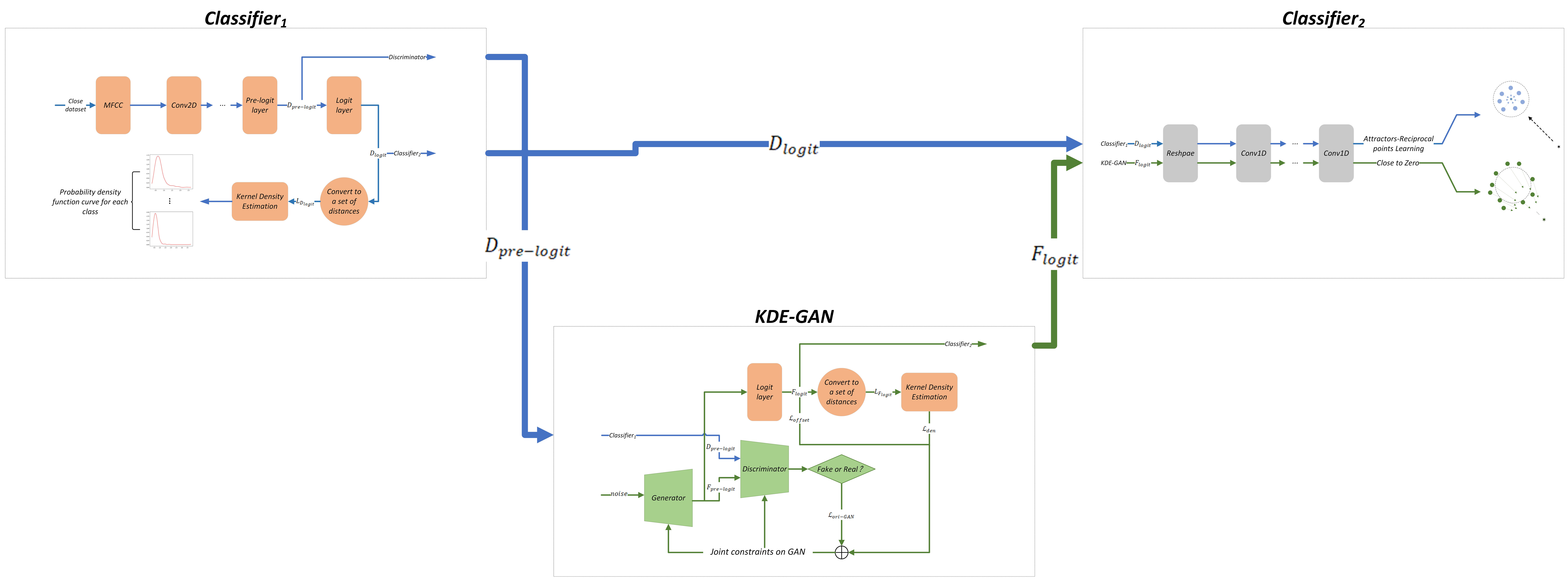Concurrently, the data in ${\mathcal{D}}_{fake}$ are constrained to remain within low-density regions. The overall process is illustrated in Figure 1, with detailed architectural components visualized in Figure 2, Figure 3 and Figure 4.

The overall algorithm flowchart delineates the primary process of our proposed algorithm, which consists of three main components: $Classifier1$, $Classifier2$, and KDE-GAN. Initially, raw samples are input into $Classifie{r}_1$ to generate pre-logit layer samples, which subsequently serve as the training set for KDE-GAN. Within the KDE-GAN framework, we employ the original GAN optimization objective while incorporating additional constraints to produce edge samples that simulate open-set scenarios. Specifically, the fake samples generated by the GAN in the pre-logit layer are mapped to the $logit$ layer, where Density Loss is computed based on the Kernel Density Estimation (KDE) of the original samples. This methodology ensures that the generated samples are situated at the boundaries of each class. To prevent the generated samples from drifting in any direction, we introduce an Offset Loss. The mapped original samples in the $logit$ layer, along with the generated outputs, are then fed into $Classifie{r}_2$. For the original samples, we utilize an Attractor–Reciprocal Point learning algorithm, whereas for the generated outputs, we encourage the results to converge toward zero. This strategy effectively ensures that closed-set data points remain proximate to attractors and distant from reciprocal points, while open-set data points are preserved within low-density regions.

3.2. Generation of Edge Samples Based on KDE-GAN

Open-set samples are inherently unknown, making it challenging to apply even the most advanced closed-set classifiers to open-set recognition problems. As discussed in the introduction, UIK samples are particularly difficult to differentiate, as they may lie closer to the sample center. In this study, we focus on distinguishing between USK and UO samples. UO samples can be effectively rejected based on their distance from the sample center, while USK samples are treated as interference items. These USK samples typically surround the clusters of known samples, significantly complicating the model’s decision-making process. To address these challenges, this section introduces the use of a KDE-constrained GAN for the generation of edge samples, aimed at enhancing the dataset. This approach seeks to improve the model’s ability to recognize and differentiate between closed-set and open-set scenarios by augmenting the training data with strategically generated edge samples. To address the challenges of high-dimensional environmental audio data points and the relatively limited dataset size compared to image datasets, which often lead to training difficulties, we propose a sample generation strategy leveraging the pre-logit layer vectors to adapt to the unique characteristics of audio samples. Specifically, the pre-logit feature representations are utilized to guide the Generative Adversarial Network (GAN) in synthesizing augmented samples. Furthermore, to ensure the quality and diversity of generated samples, Kernel Density Estimation (KDE) is introduced as a constraint during GAN training, effectively regularizing the generation of boundary samples that lie near the decision regions of the classifier. This approach enhances the model’s robustness and generalizability by enriching the training distribution while maintaining alignment with the intrinsic statistical properties of the original audio data.

GANs consist primarily of a Generator and a Discriminator. The Generator takes a random noise distribution $p_{fake}\left(z\right)$ and generates synthetic data that closely resemble the original sample distribution $p_{ori}\left(x\right)$ in order to deceive the Discriminator. The Discriminator’s role is to assess whether the input sample originates from the real data or the generated data. This setup embodies a two-player game concept, where adversarial training between the Generator and the Discriminator drives the optimization process. The optimization objective function of the original GAN is defined as follows:

$$\begin{array}{cc}\hfill & \underset{G}{min}\underset{D}{max}V\left(G,D\right)\hfill \\ \hfill =& E_{x\sim p_{ori}x}\left[logD\left(x\right)\right]+E_{z\sim p_{fake}z}\left[log1-D\left(G\left(z\right)\right)]\right.,\hfill \end{array}$$

(6)

where $D\left(x\right)$ represents the probability that a sample comes from $p_{ori}\left(x\right)$ and $1-D\left(G\right(z\left)\right)$ represents the probability that a sample comes from $p_{fake}\left(z\right)$.

Given that environmental audio datasets are typically much smaller than image or text datasets, directly performing data augmentation on raw samples presents significant challenges. To address this, this study proposes an alternative strategy: performing data augmentation on the output of a specific neural network layer.

In Generative Adversarial Networks (GANs), the generator typically involves a dimension-increasing process to effectively capture the structural patterns of the data distribution, rather than relying directly on high-dimensional input at this stage. This approach helps avoid overfitting while improving generation efficiency. To ensure the generated samples maintain the same dimensionality as the training samples, the generator’s input dimension is usually kept low. Considering the limited number of categories involved in this study’s recognition task, the generator’s input dimension is further reduced, posing certain challenges for the GAN’s architectural design.

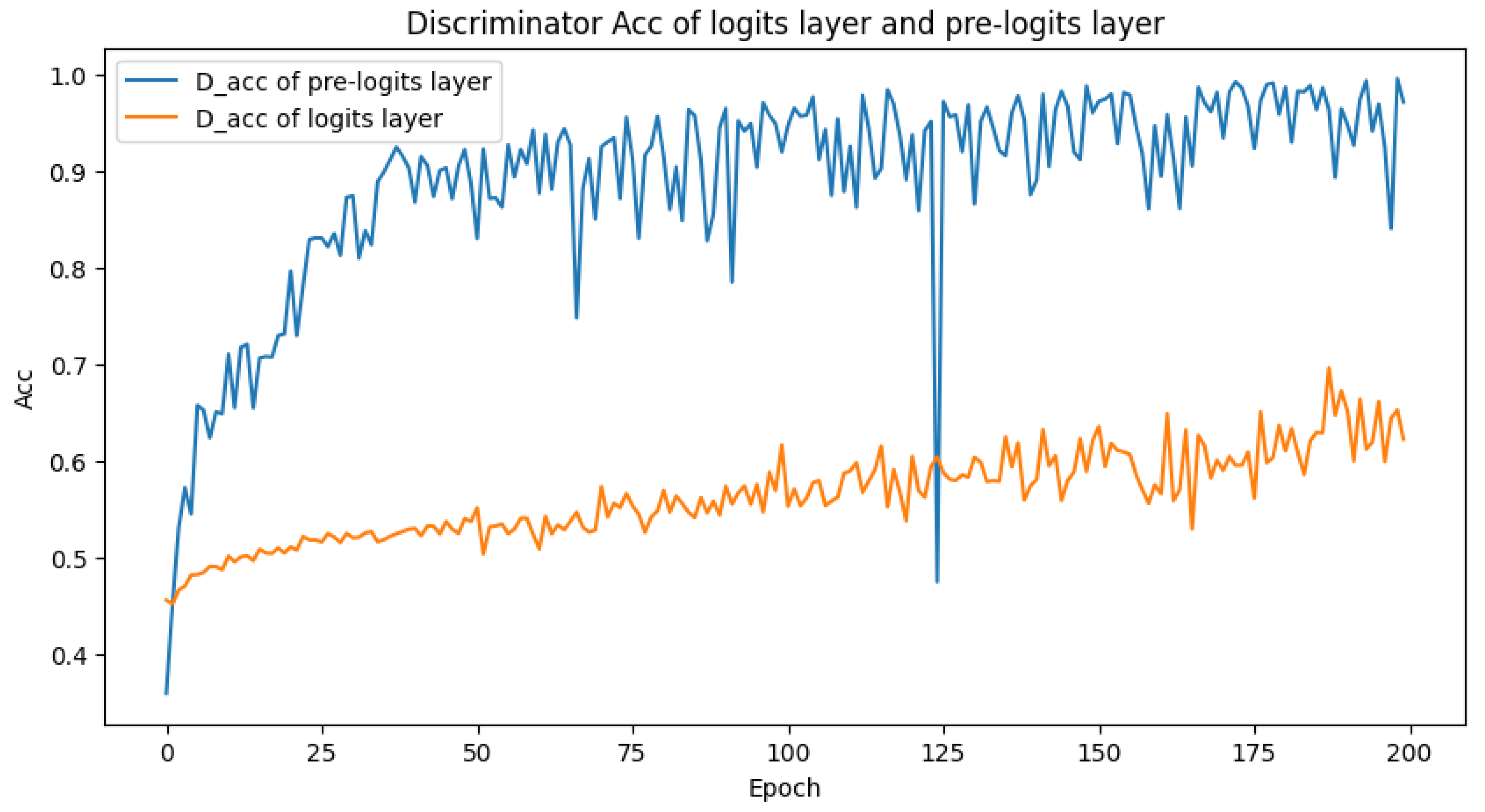
Therefore, this research proposes using the pre-logit layer output (i.e., the layer preceding the logit output) as the GAN’s input to optimize the generator design. In this section, since the generated samples are high-dimensional vectors that are difficult to evaluate directly, we leverage the discriminator’s accuracy as an indirect measure of the generator’s performance. This is possible because the generator and discriminator engage in a zero-sum game during training. Under the constraint that the generator’s input dimension must be smaller than its output dimension, samples are generated at both the pre-logit and logit layers, with the discriminator’s accuracy curves visualized as shown in Figure 5.

So as illustrated in Figure 5, which displays the accuracy curves of the discriminator during GAN training on samples from both the $logit$ layer and the pre-logit layer, it is clear that the small dimensionality of the $logit$ layer in environmental recognition tasks where most datasets contain only a few classes poses a risk of overfitting when the latent space dimension of the GAN is only slightly larger. Conversely, if the latent space dimension is smaller than that of the $logit$ layer, the GAN network has an insufficient number of parameters, leading to failure in convergence.

In contrast, generating samples at the pre-logit layer enables the attainment of higher-quality results with the GAN. Consequently, the subsequent sections focus on training the GAN using a dataset ${\mathcal{D}}_k$ composed of outputs from the pre-logit layer.

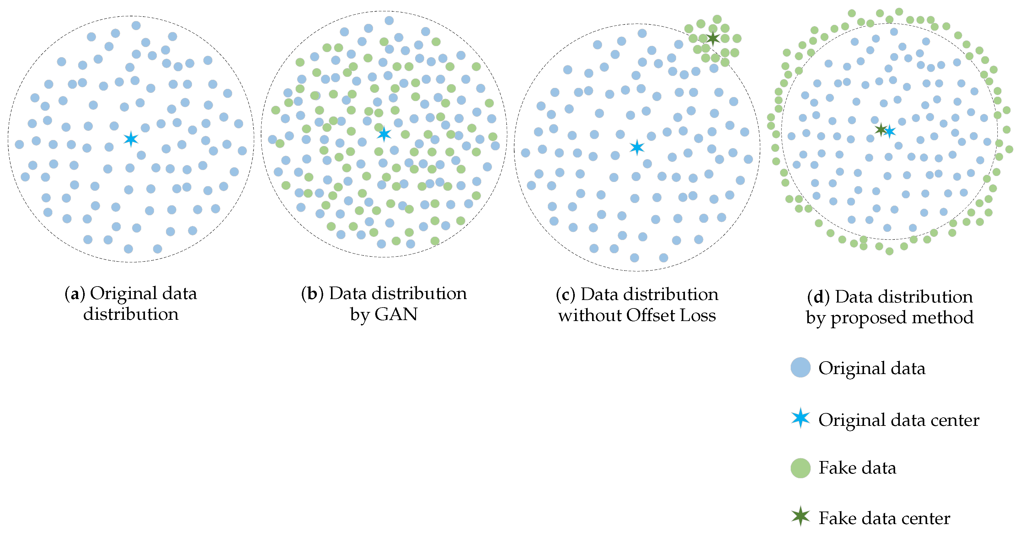
However, the aforementioned optimization objective function merely compels the fake data distribution to approximate the original sample distribution, as illustrated in Figure 6a,b. Consequently, generating edge samples using this function alone proves challenging, necessitating additional optimization strategies.

Given that the $logit$ layer dataset ${\mathcal{D}}_k=\{x_1,x_2,\dots ,x_i,\dots ,x_n\}$ comprises high-dimensional vectors and considering that environmental audio datasets are typically smaller than image or text datasets, fitting their distribution poses a challenge. Furthermore, generating edge data for each class of samples is essential. If the original data are represented as several hyperspherical distributions, edge samples are located at the peripheries of these hyperspheres, complicating visualization. To facilitate modeling, we partition ${\mathcal{D}}_k$ into C subsets $\{{\mathcal{D}}_{k1},{\mathcal{D}}_{k2},\dots ,{\mathcal{D}}_{ki},\dots ,{\mathcal{D}}_{kC}\}$, compute the center points $\{a_{k1},a_{k2},\dots ,a_{ki},\dots ,a_{kC}\}$ for each class, and derive the corresponding distances to form a new one-dimensional dataset $L_k=\{L_{k1},L_{k2},\dots ,L_{ki},\dots ,L_{kC}\}$, where $L_{ki}$ represents the distance set for the ith class. For any $l_i\in L_{ki}$, the calculation formula is as follows:

$$l_i=d(x_i,a_{ki}),$$

(7)

where $d(·,·)$ is the distance function, $x_i\in {\mathcal{D}}_{ki}$, and $a_{ki}$ is the corresponding center point.

We reduce high-dimensional data points to one-dimensional representations, facilitating modeling and enabling histogram visualization, as illustrated in Figure 7a. The edge samples we aim to generate correspond to those located at the tail of this histogram. However, as previously noted, the optimization objective defined in Equation (6) of the original GAN only ensures that the generated samples approximate the original data distribution, complicating the direct acquisition of boundary samples. Consequently, the generated samples from the original GAN are also represented as a distance histogram, as depicted in Figure 7b.

We now introduce the Kernel Density Estimation (KDE) method to model $L_{ki}$. We let $F_{ki}\left(x\right)$ denote the cumulative distribution function of $L_{ki}$ and let $f_{ki}\left(x\right)$ represent its probability density function. Then

$$\left\{\begin{array}{c}{F}_{ki}\left(x_{i-1}\le x\le x_i\right)\left.={\int }_{x_{i-1}}^{x_i}{f}_{ki}\left(x\right)dx\right)\\ f_{ki}\left(x_i\right)=\underset{h\to 0}{lim}{\displaystyle \frac{F_{ki}\left(x_i+h\right)-F_{ki}\left(x_i-h\right)}{2h}}\end{array}\right..$$

(8)

However, discrete data points alone do not allow us to derive analytical expressions for $F_{ki}\left(x\right)$ and $f_{ki}\left(x\right)$. Therefore, we introduce $\stackrel{\sim }{F_{ki}}\left(x\right)$, which serves as the empirical distribution function corresponding to $F_{ki}\left(x\right)$.

$$\stackrel{\sim }{F_{ki}}\left(x\right)={\displaystyle \frac{{\sum }_{j=1}^n{I}_{X_j\le x}}{n}}.$$

(9)

$\stackrel{\sim }{F_{ki}}\left(x\right)$ is an unbiased estimation of $F_{ki}\left(x\right)$. It approximates $P\left(X_j\le x\right)$ by the ratio of the number of times $P\left(X_j\le x\right)$ occurs in n observations to n. Substituting this into $f_{ki}\left(x_i\right)$, we can obtain its approximate estimation $\stackrel{\sim }{f_{ki}}\left(x_i\right)$:

$$\begin{array}{cc}\hfill \stackrel{\sim }{f_{ki}}\left(x_i\right)& =\underset{h\to 0}{lim}{\displaystyle \frac{\stackrel{\sim }{F_{ki}}\left(x_i+h\right)-\stackrel{\sim }{F_{ki}}\left(x_i-h\right)}{2h}}\hfill \\ & =\underset{h\to 0}{lim}{\displaystyle \frac{{\sum }_{j=1}^n{I}_{X_{j-h}\le x\le X_{j+h}}}{2nh}}.\hfill \end{array}$$

(10)

Upon introducing the kernel function, Equation (10) can be transformed into

$$\begin{array}{cc}\hfill \stackrel{\sim }{f_{ki}}\left(x_i\right)& =\underset{h\to 0}{lim}{\displaystyle \frac{{\sum }_{j=1}^n{I}_{X_{j-h}\le x\le X_{j+h}}}{nh}}\hfill \\ & ={\displaystyle \frac{{\sum }_{j=1}^{n}K\left(\frac{x-x_j}{h}\right)}{nh}}\hfill \\ & ={\displaystyle \frac{1}{n}}\sum _{j=1}^n{K}_h\left(x-x_j\right).\hfill \end{array}$$

(11)

In this context, $K(·)$ represents the kernel function and h denotes the bandwidth of the kernel function.

After fitting the probability density function, we can calculate the probability of data points falling within $d_i\le d\le d_j$.

$$p\left(d_i\le d\le d_j\right)={\int }_{d_i}^{d_j}\stackrel{\sim }{f_{ki}}\left(x_i\right)dx.$$

(12)

What we need to generate are data points surrounding each class sample, specifically points that are farther from the corresponding center. This means that $p\left(0\le d\le d\left(x_{fake},a_{ki}\right)\right)$ should be larger. To address this, we propose the Density Loss:

$$\begin{array}{cc}\hfill {\mathcal{L}}_{den}=& -{\displaystyle \frac{1}{N}}\sum _{j=1}^N\left(y_j·log\left(p_{d\le d(x_{fake},a_{ki})}\right)\right.\hfill \\ \hfill & \left.+(1-y_j)·log\left(1-p_{d\le d(x_{fake},a_{ki})}\right)\right),\hfill \end{array}$$

(13)

where $y_j=1$, $x_{fake}=G\left(z\right)$, and $a_{ki}$ represents the center of the corresponding class; $d(·,·)$ is the distance function.

Additionally, we aim for the generated samples to be as uniformly distributed as possible on the surface of the corresponding class hypersphere. Relying solely on ${\mathcal{L}}_{den}$ as a constraint may cause the network output to shift in a specific direction on the hypersphere, rather than achieving a uniform distribution across its surface, as illustrated in Figure 6c. In such instances, the constraint of ${\mathcal{L}}_{den}$ may still be satisfied. Therefore, we must introduce an additional constraint to guide the network toward convergence in the desired direction.

In fact, we can conceptualize the desired generated fake samples as a spherical shell surrounding a hypersphere. This spherical shell should share the same center as the hypersphere of the corresponding class. By constraining the distance between the center of the shell and the center of the hypersphere, we can ensure that the generated fake samples are uniformly distributed on the surface of the hypersphere. To facilitate this, we propose the Offset Loss:

$${\mathcal{L}}_{offset}=\sum _{i=1}^C{\left.{\left(x\right.}_{{center\_batch}_i}-a_{ki}\right)}^2,$$

(14)

where $x_{{cente{r}_{b}atch}_i}$ is the mean of the samples belonging to the ith class within the current batch size.

By incorporating ${\mathcal{L}}_{offset}$, any shift of the generated samples within a batch in a particular direction results in an increased loss. This, in conjunction with ${\mathcal{L}}_{den}$, compels the generated samples to be as uniformly distributed as possible on the surface of the spherical shell surrounding the hypersphere.

In summary, we propose an optimization objective function for Generative Adversarial Network (GAN) specifically tailored for generating edge samples:

$$\begin{array}{cc}\hfill \underset{G}{min}\underset{D}{max}(E_{x\sim p_{\mathrm{ori}}\left(x\right)}\left[logD\left(x\right)\right]& +E_{z\sim p_{\mathrm{fake}}\left(z\right)}\left[log\left(1-D\left(G\right(z\left)\right)\right)\right])\hfill \\ \hfill & +\alpha ·{\mathcal{L}}_{\mathrm{den}}+\beta ·{\mathcal{L}}_{\mathrm{offset}}.\hfill \end{array}$$

(15)

Utilizing the improved optimization objective function to generate fake samples, we classify them by distance, calculate the distance from the center for each sample, and present the results as a histogram, as illustrated in Figure 7c. A comparison between Figure 7b,c confirms that the enhanced generator is more effective in producing samples situated at the edges compared to the original GAN.

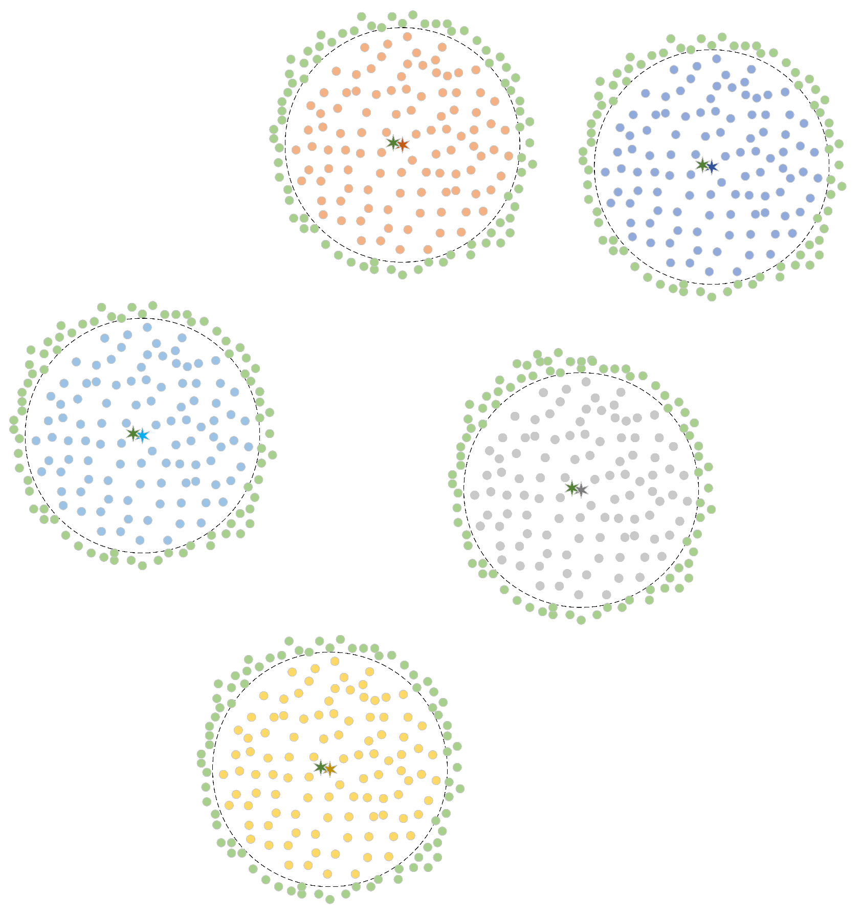
In this context, we generate edge data for each sample category, as illustrated in Figure 8. This approach enables us to leverage the data to simulate open-set samples, thereby facilitating data augmentation.

3.3. Attractor–Reciprocal Point Learning

Before introducing our method, it is essential to review the reciprocal point algorithm [18,26]. For a given class sample set ${\mathcal{D}}_k=\left\{x_1,x_2,\dots ,x_i,\dots ,x_n\right\}$, which is partitioned into C distinct subsets ${\mathcal{D}}_k=\{{\mathcal{D}}_{k1}\bigcup \dots \bigcup {\mathcal{D}}_{kC}\}$ based on labels, we define C reciprocal points $\left\{{\mathcal{P}}^1,\dots ,{\mathcal{P}}^C\right\}$. The training objective for the reciprocal points is to maximize the difference between each training subset ${\mathcal{D}}_{ki}$ and its corresponding reciprocal point ${\mathcal{P}}^i$. Therefore, the relationship between data points in other subsets ${\mathcal{D}}_{kj,j\ne i}$ and the unknown sample set ${\mathcal{D}}_{uk}$ with respect to the reciprocal point ${\mathcal{P}}^i$ must satisfy

$$max\left(\zeta \left({\mathcal{D}}_{kj,j\ne i}\bigcup {\mathcal{D}}_{uk},{\mathcal{P}}^i\right)\right)\le d,\forall d\in \zeta \left({\mathcal{D}}_{ki},{\mathcal{P}}^i\right),$$

(16)

where $\zeta (·,·)$ denotes a function used to compute their difference.

In [18,26], the authors use euclidean distance $d_e$ and the dot product $d_d$ to describe this difference $d\left(g_1\left(x_i\right),{\mathcal{P}}^i\right)$.

$$\begin{array}{cc}\hfill d_e\left(g_1\left(x_i\right),{\mathcal{P}}^i\right)& ={\displaystyle \frac{1}{m}}{∥g_1\left(x_i\right)-{\mathcal{P}}^i∥}_2^2,\hfill \\ \hfill d_d\left(g_1\left(x_i\right),{\mathcal{P}}^i\right)& =g_1\left(x_i\right)·{\mathcal{P}}^i,\hfill \\ \hfill d\left(g_1\left(x_i\right),{\mathcal{P}}^i\right)& =d_e\left(g_1\left(x_i\right),{\mathcal{P}}^i\right)-d_d\left(g_1\left(x_i\right),{\mathcal{P}}^i\right).\hfill \end{array}$$

(17)

We can predict a sample’s class based on this difference: the greater the distance from a reciprocal point, the higher the probability that the sample belongs to that class. Conversely, if the distance is below a certain threshold, the sample can be classified as unknown. These measures aim to minimize the empirical risk ${\mathcal{R}}_{exp}$. Additionally, the author implements an Adversarial Margin Constraint to limit the open space within a bounded range, addressing the open-space risk ${\mathcal{R}}_O$. Despite the effectiveness of the aforementioned methods, several issues persist: (1) Reciprocal points are randomly selected and updated via backpropagation, making it susceptible to local optima; (2) The training process primarily emphasizes distancing data points from their corresponding reciprocal points without addressing intra-class relationships, which may result in a wider distribution of known class samples in the open space and an elevated open set risk; (3) The generation of edge samples is not accounted for.

In our algorithm, each class is assigned an attractor ${\mathcal{A}}^i$ and a reciprocal point ${\mathcal{P}}^i$. The role of the reciprocal point is to maximize the distance from the samples, while the attractor ensures that the distribution of samples within a class is minimized. Furthermore, by incorporating edge samples from ${\mathcal{D}}_{fake}$, we restrict the open set data to a low-density region. For each sample x in the known set ${\mathcal{D}}_k$, we first extract its feature vector $g_1\left(x\right)$ through the neural network. We then compute the distances to each pair of attractor and reciprocal points, classifying the sample as belonging to the class whose attractor is closest and whose reciprocal point is farthest, expressed as follows:

$$\left\{\begin{array}{c}x\in i\\ i={argmax}_{j=1}^C\left(-d\left(g_1\left(x\right),{\mathcal{A}}^i\right)+d\left(g_1\left(x\right),{\mathcal{P}}^i\right)\right)\end{array}\right.,$$

(18)

where $d(·,·)$ represents a certain distance metric.

Therefore, the probability that x belongs to class i can be assessed based on the distances between the sample’s feature vector $g_1\left(x\right)$ and the attractor ${\mathcal{A}}^i$ as well as the reciprocal point ${\mathcal{P}}^i$ of class i:

$$\left\{\begin{array}{cc}p(x\in i\mid x)\propto \hfill & d(g_1\left(x\right),{\mathcal{P}}^i),\hfill \\ p(x\in i\mid x)\propto -\hfill & d(g_1\left(x\right),{\mathcal{A}}^i).\hfill \end{array}\right.$$

(19)

To satisfy the properties of non-negativity and normalization of probabilities, we can provide two different probability expressions:

$$\left\{\begin{array}{ccc}\hfill p\left(x\in i|x,\mathcal{A},\mathcal{P}\right)& ={\displaystyle \frac{exp\left(\gamma ·\left(d\left(g_1\left(x\right),{\mathcal{P}}^i\right)-d\left(g_1\left(x\right),{\mathcal{A}}^i\right)\right)\right)}{{\sum }_{j=1}^{C}exp\left(\gamma ·\left(d\left(g_1\left(x\right),{\mathcal{P}}^j\right)-d\left(g_1\left(x\right),{\mathcal{A}}^j\right)\right)\right)}}\hfill & \hfill \left(1\right)\\ \hfill p\left(x\in i|x,\mathcal{A},\mathcal{P}\right)& ={\displaystyle \frac{exp\left(\gamma ·d\left(g_1\left(x\right),{\mathcal{P}}^i\right)\right)}{{\sum }_{j=1}^{C}exp\left(\gamma ·d\left(g_1\left(x\right),{\mathcal{P}}^j\right)\right)}}+{\displaystyle \frac{exp\left(\gamma ·\frac{1}{d\left(g_1\left(x\right),{\mathcal{A}}^i\right)+\sigma }\right)}{{\sum }_{j=1}^{C}exp\left(\gamma ·\frac{1}{d\left(g_1\left(x\right),{\mathcal{A}}^j\right)+\sigma }\right)}}\hfill & \hfill \left(2\right)\end{array}\right.,$$

(20)

where $\sigma$ is a small value introduced to ensure that the denominator is not zero.

Equation (20)-1 primarily measures the probability by examining the difference in distances between the feature vector of the sample point, $g_1\left(x\right)$, to the reciprocal point and the attractor. In contrast, Equation (20)-2 assesses the probability by considering the distances from the feature vector $g_1\left(x\right)$ to the reciprocal point and the attractor separately. Both equations adhere to the aforementioned probability constraints and necessitate appropriate selection and differentiation processes.

Firstly, the attractor should be positioned as centrally as possible within a class of sample points, while the reciprocal point should be maximally distinct from these samples. Thus, the relative position and angle of both the reciprocal point and the attractor in the feature space are critical. To minimize open-space risk, it is essential to cluster each class of samples tightly while also limiting the overall distribution range of all samples, effectively reducing the spread of known samples in open space. When employing Equation (20)-1 for probability calculations, the constraint only considers the difference $d=d\left(g_1\left(x\right),{\mathcal{P}}^i\right)-d\left(g_1\left(x\right),{\mathcal{A}}^i\right)$. This may lead to situations where $d\left(g_1\left(x\right),{\mathcal{P}}^i\right)$ becomes excessively large, diminishing the relevance of $d\left(g_1\left(x\right),{\mathcal{A}}^i\right)$. Consequently, even if $d\left(g_1\left(x\right),{\mathcal{A}}^i\right)$ is substantial, it might still satisfy the equation, inadvertently expanding the sample distribution range and increasing open-space risk. Our training objective should ensure that sample points lie within the vicinity of both the attractor and reciprocal point, remaining close to the attractor while distancing from the reciprocal point, as illustrated in Figure 9.

Therefore, Equation (20)-2 better meets our training expectations. We can then define the Attractor and Reciprocal Point Distance Cross-Entropy Loss as follows:

$$\left\{\begin{array}{cc}\hfill {\mathcal{L}}_{ARDCE}& =-\sum _{i=1}^{C}log\left(p\left(x\in i|x,\mathcal{A},\mathcal{P}\right)\right)\hfill \\ \hfill p\left(x\in i|x,\mathcal{A},\mathcal{P}\right)& ={\displaystyle \frac{exp\left(\gamma ·d\left(g\left(x\right),{\mathcal{P}}^i\right)\right)}{{\sum }_{j=1}^{C}exp\left(\gamma ·d\left(g\left(x\right),{\mathcal{P}}^j\right)\right)}}+{\displaystyle \frac{exp\left(\gamma ·\frac{1}{d\left(g\left(x\right),{\mathcal{A}}^i\right)+\sigma }\right)}{{\sum }_{j=1}^{C}exp\left(\gamma ·\frac{1}{d\left(g\left(x\right),{\mathcal{A}}^j\right)+\sigma }\right)}}\hfill \end{array}\right..$$

(21)

In this study, we employ Euclidean distance $d_e$ to quantify the positional distance between the reciprocal points, attractors, and sample points. Additionally, we utilize the dot product $d_d$ to assess the angular difference between the reciprocal points and sample points in the feature space, specifically

$$\begin{array}{c}\hfill \left\{\begin{array}{cc}d\left(g_1\left(x\right),{\mathcal{P}}^i\right)=& {∥g_1\left(x_i\right)-{\mathcal{P}}^i∥}_2^2-\lambda g_1\left(x_i\right)·{\mathcal{P}}^i\\ d\left(g_1\left(x\right),{\mathcal{A}}^i\right)=& {∥g_1\left(x_i\right)-{\mathcal{A}}^i∥}_2^2\end{array}\right..\end{array}$$

(22)

Similarly, we implement a boundary R to restrict the overall distribution range of the sample points:

$${\mathcal{L}}_O=max\left({∥g_1\left(x\right)-{\mathcal{P}}^i∥}_2^2-R,0\right).$$

(23)

The loss functions ${\mathcal{L}}_{ARDCE}$ and ${\mathcal{L}}_O$ are designed to constrain the data within ${\mathcal{D}}_k$. Additionally, we utilize the edge sample dataset ${\mathcal{D}}_{fake}$, obtained in Section 3.2, to approximate open-set samples. Our objective is to maintain unknown samples in a low-density region while pushing known samples away. To achieve this, we constrain the $l_2-norm$ of the samples in ${\mathcal{D}}_{fake}$ to approach zero, specifically

$${\mathcal{L}}_{l_2}=\sum _{i=1}^N{\parallel x_{fake}\parallel }_2.$$

(24)

So the total training loss is

$$\mathcal{L}={\mathcal{L}}_k+\beta {\mathcal{L}}_{fake}=\left({\mathcal{L}}_{ARDCE}+\alpha {\mathcal{L}}_O\right)+\beta {\mathcal{L}}_{l_2},$$

(25)

where $\alpha$ and $\beta$ are hyperparameters that control the weights. Clearly, the computation process of $\mathcal{L}$ is differentiable.

In the original reciprocal point algorithm, the reciprocal points for each class were initialized randomly. We contend that this random initialization, in conjunction with network updates, is susceptible to local optima. Since the ultimate goal of training is to separate samples of different classes from their respective reciprocal points, the selection of reciprocal points should adhere to a systematic pattern. Given that the activation function used in the models for this experiment is ReLU, which discards negative values, we can strategically position the reciprocal points in opposite quadrants or along the same coordinate axis in opposite directions relative to the sample feature vectors. This approach maximizes both positional and angular differences. Thus, we propose using orthogonal basis vectors for initialization:

$$\left\{\begin{array}{c}\mathcal{P}=\left({\mathcal{P}}^1,{\mathcal{P}}^2,\dots ,{\mathcal{P}}^i,\dots ,{\mathcal{P}}^C\right)=\left({\alpha }_1·e_1,\dots ,{\alpha }_i·e_i,\dots ,{\alpha }_C·e_C\right)\\ e_1=(1,0,\dots ,0,\dots ,0)\\ \dots \\ e_C=(0,0,\dots ,0,\dots ,1)\end{array}\right.,$$

(26)

where $e_i$ is the basis vector in that space and $\alpha$ is the reciprocal point coefficient.

In other words, we set the reciprocal points in the negative direction of the C coordinate axes. Since the attractors and the reciprocal points are relative in terms of angle and position, the optimal attractors $\mathcal{A}$ should satisfy

$$\mathcal{A}=\lambda ·\mathcal{P},$$

(27)

where $\lambda$ is the scaling factor between the attractors $\mathcal{A}$ and the reciprocal points $\mathcal{P}$.

3.4. Network Architecture

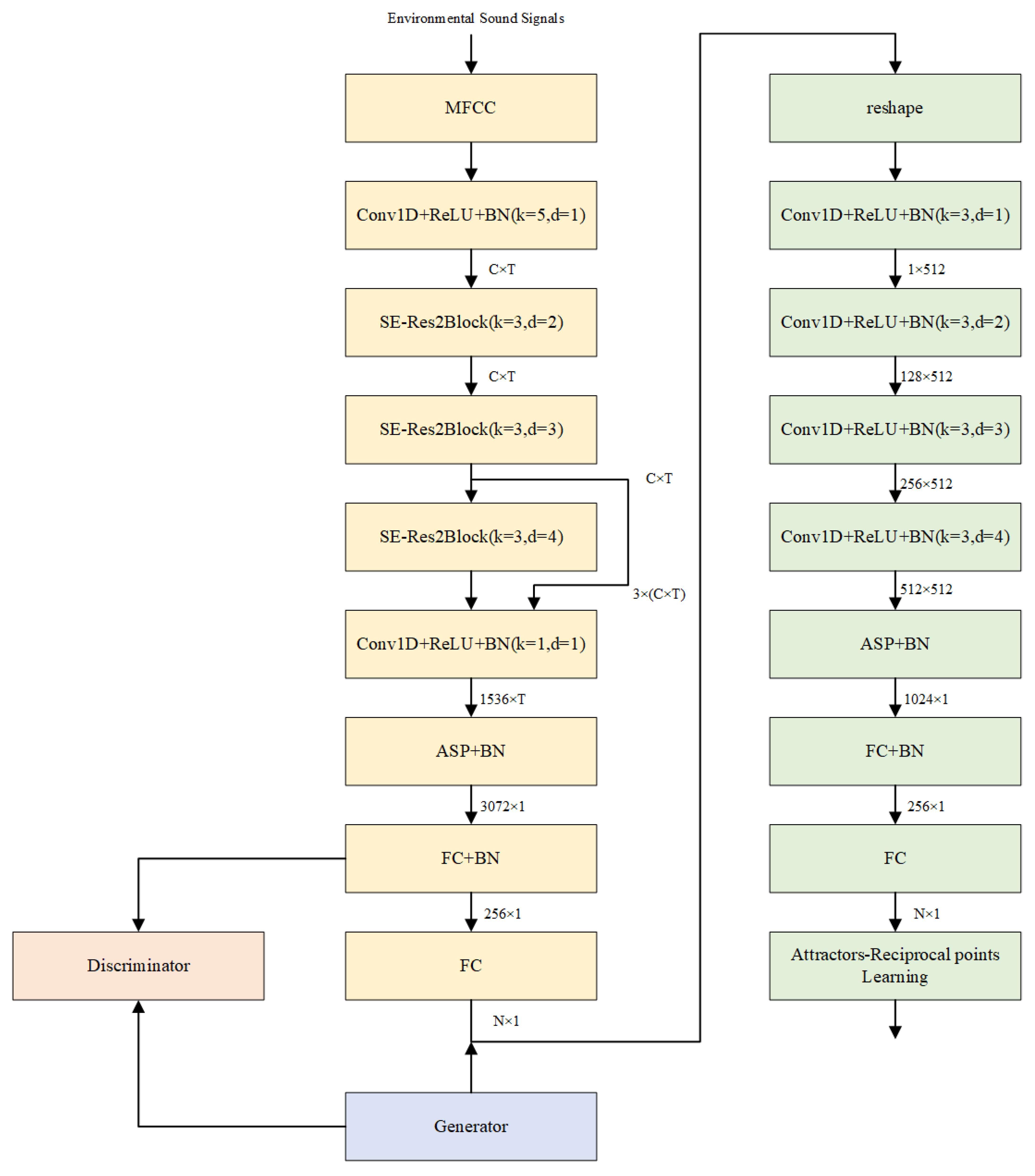
The previous sections provide a detailed introduction to the proposed open-set recognition algorithm. This section presents the corresponding network architecture, as shown in Figure 10.

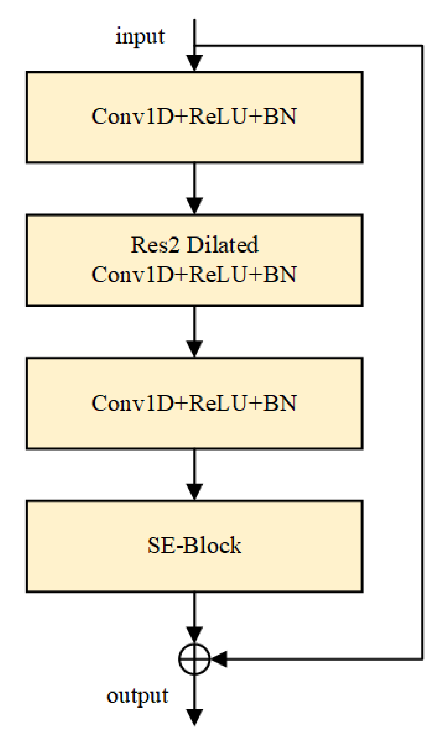
The environmental audio signal first undergoes Mel-Frequency Cepstral Coefficient (MFCC) feature extraction, which is then fed into $Classifie{r}_1$. $Classifie{r}_1$ employs the ECAPA-TDNN model [1], a speaker recognition architecture based on time-delay neural networks. The model comprises three main modules: the SE-Res2Block (Squeeze-and-Excitation Res2Block) module (illustrated in Figure 11), the Multi-Layer Feature Aggregation and Summation (MFA) module, and the Attentive Statistic Pooling (ASP) module.

The MFCC features are initially transformed via a Conv1D+ReLU+Batch Normalization (BN) layer to adjust their dimensionality. Subsequently, three SE-Res2Block modules with dilation rates of k = 2, 3, 4, respectively, perform squeeze-and-excitation operations. The outputs of these SE-Res2Block modules with varying dilation rates are concatenated through a Conv1D+ReLU layer for multi-layer feature aggregation (MFA), generating refined features for attentive statistical pooling. These features are then aggregated and pooled via the ASP module. The pooled features pass through a fully connected (FC) layer with 256 nodes to produce the pre-logit output vector. A subsequent FC layer reduces the dimensionality to N, yielding the logit output vector, where N denotes the number of known classes. Additionally, the pre-logit output vector is fed into the $Discriminator$ for adversarial training, while the logit output vector, combined with the boundary samples generated by the $Generator$, is input to $Classifie{r}_2$.

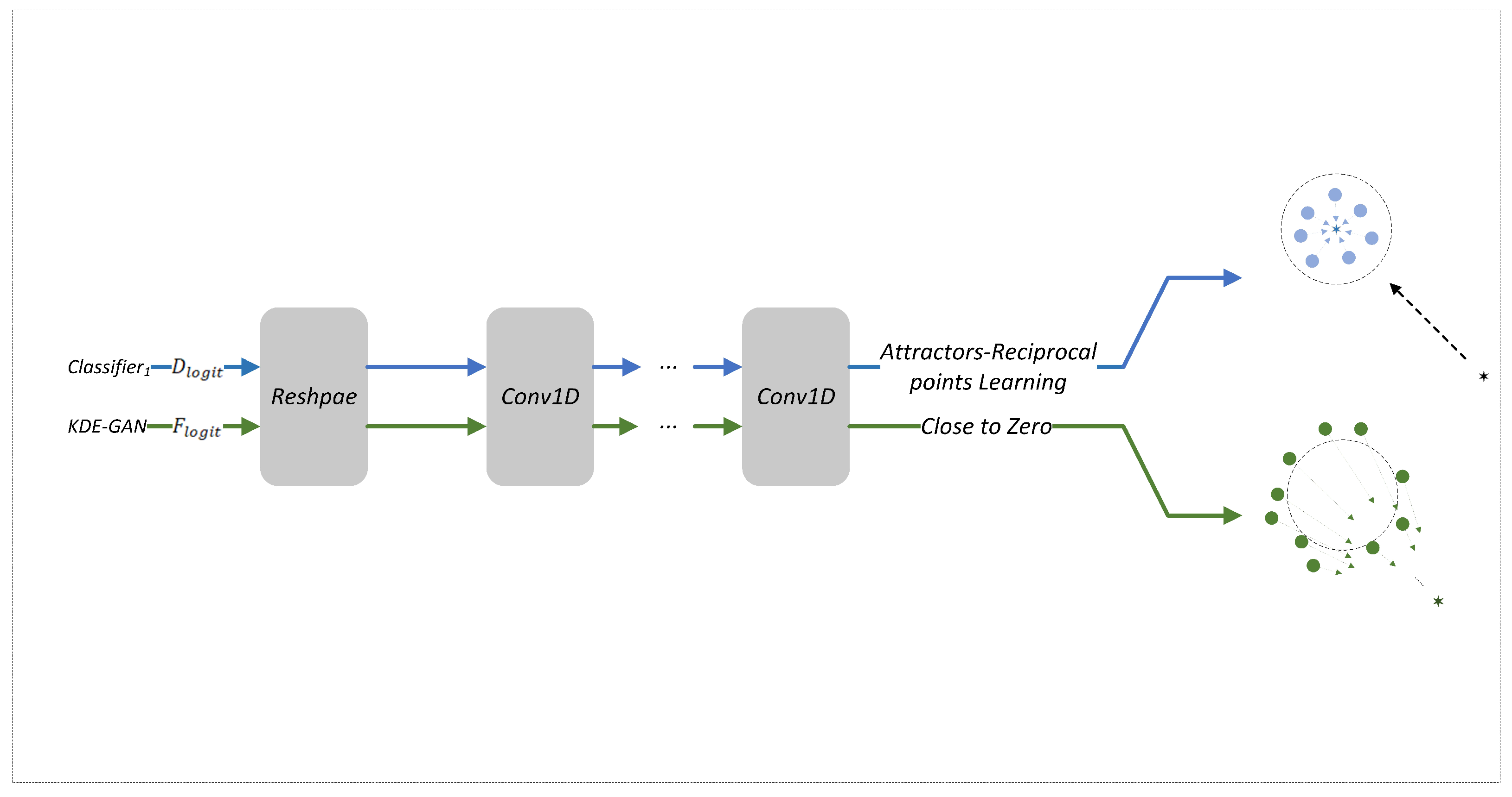
For $Classifie{r}_2$, the input vectors first undergo dimensionality transformation to ensure a feature dimension of 3. A Conv1D+ReLU+BN layer then maps the features to 512 dimensions while retaining a channel dimension of 1. This is followed by three sequential Conv1D+ReLU+BN layers that progressively expand the channel dimensions to 128, 256, and 512, with dilation rates incrementally increased to capture multi-scale temporal features. After feature extraction, the ASP module compresses the dimensionality to 1024. Two FC layers further reduce the dimensionality to N. The final output undergoes Attractor–Reciprocal Point Learning to update the network parameters.

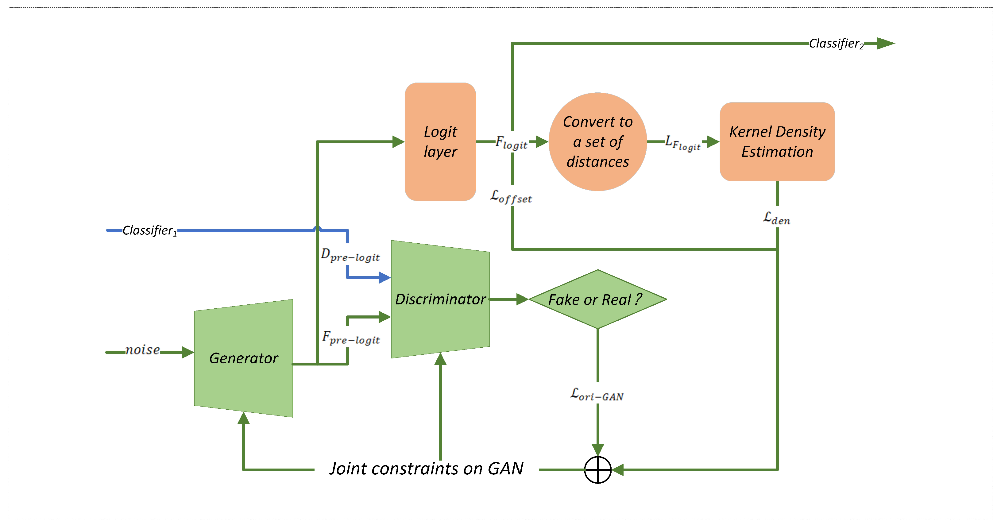
In the $Generator$ (Figure 12), the input random noise (dimension 100) passes through four Conv1D+ReLU+BN and Dropout modules, with intermediate dimensions of 2048, 1024, 512, and 1024. A final 1D convolutional layer reduces the dimensionality to 256, producing synthetic data points.

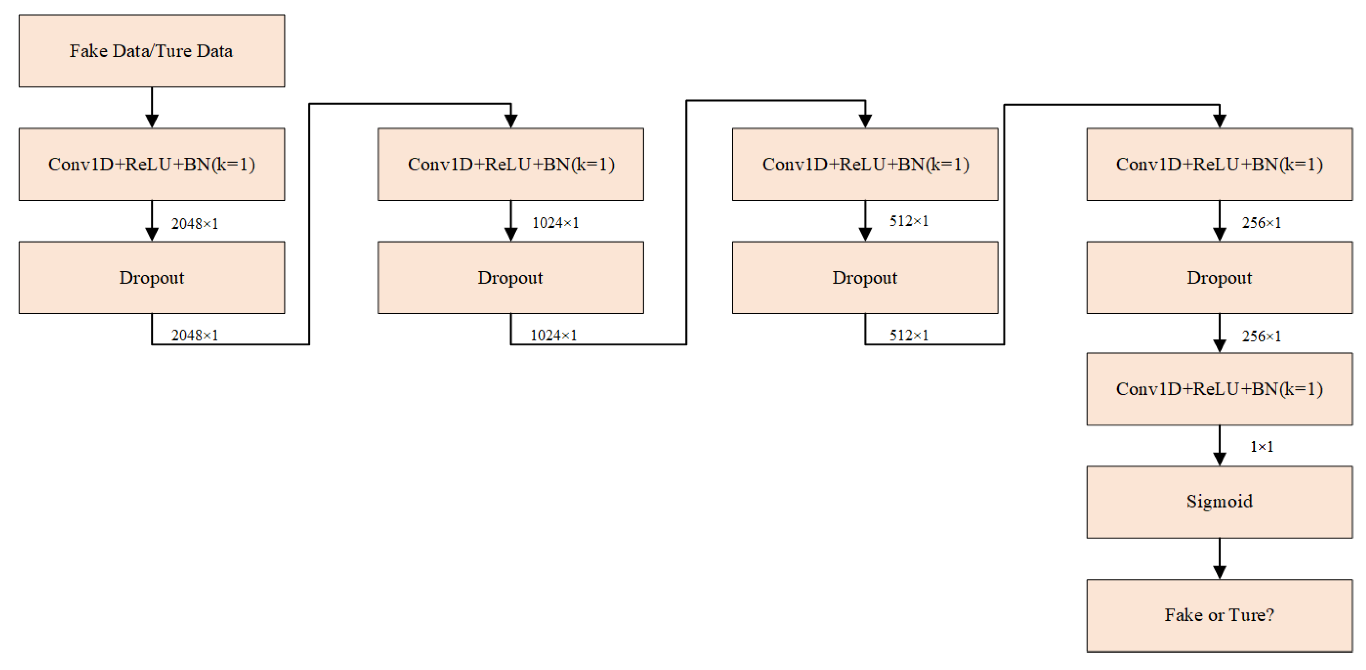
In the $Discriminator$ (Figure 13), the input consists of generated data points and the pre-logit output vector (both 256-dimensional). These pass through four Conv1D+ReLU+BN and Dropout modules with intermediate dimensions of 2048, 1024, and 512. A final 1D convolutional layer reduces the dimensionality to 1, followed by a Sigmoid activation function to map outputs to the range [0, 1].

4. Experiment and Result

In this section, we first outline the selection of the backbone, the dataset, and its partitioning method, along with the preprocessing techniques and other foundational aspects. Finally, we detail the process and results of the comparative experiments.

4.1. Basic Experimental Settings

In this experiment, the network architecture is shown in Section 3.4. The known class datasets include UrbanSound8K [27] (split into training and testing sets in a 9:1 ratio), AudioEventDataset [28], and TUT Acoustic Scenes 2017 [29] (partitioned according to the officially provided Fold 1). Categories from ESC-50 [30] that do not overlap with any of the aforementioned datasets are chosen as unknown samples, totaling 46 classes for UrbanSound8K, 37 classes for AudioEventDataset, and 49 classes for TUT. Consequently, based on the openness calculation formula

$$O^{*}=1-\sqrt{{\displaystyle \frac{2\times {num}_{train}}{{num}_{test}+{num}_{target}}}},$$

(28)

where ${num}_{train}$ denotes the number of classes involved in training, ${num}_{test}$ denotes the number of classes involved in testing (including both known and unknown classes), and ${num}_{target}$ denotes the number of known classes involved in testing, the openness of this experiment is as follows:

$$O_{US8K}^{*}=1-\sqrt{{\displaystyle \frac{2\times {num}_{train}}{{num}_{test}+{num}_{target}}}}=1-\sqrt{{\displaystyle \frac{2\times 10}{56+10}}}=0.9322$$

(29)

$$O_{AED}^{*}=1-\sqrt{{\displaystyle \frac{2\times {num}_{train}}{{num}_{test}+{num}_{target}}}}=1-\sqrt{{\displaystyle \frac{2\times 28}{65+28}}}=0.9195$$

(30)

$$O_{TUT}^{*}=1-\sqrt{{\displaystyle \frac{2\times {num}_{train}}{{num}_{test}+{num}_{target}}}}=1-\sqrt{{\displaystyle \frac{2\times 15}{64+15}}}=0.9307$$

(31)

Finally, for the evaluation metrics, we choose to use AUROC [31] and OSCR [32] to comprehensively assess the performance of the algorithm.

4.2. Results

The distance histogram of the generated edge samples based on the method proposed in this paper is shown in Figure 7 of Section 3.2. Analysis of the histogram reveals that the original GAN-generated samples have difficulty generating edge samples, whereas the method proposed in this paper is more effective in generating edge samples. Further analysis indicates that the distribution of the generated edge samples is highly similar to that of open-set samples.

Taking the UrbanSound8K dataset as an example, Figure 14 illustrates the t-SNE visualization of both the pre-logit output vectors from $Classifie{r}_1$ and the generated samples. The results demonstrate that the generated samples are distributed around the periphery of known samples while maintaining minimal overlap with them, which aligns with our objective of generating samples with distinct distributions from known classes. This provides empirical evidence that our proposed data augmentation method can effectively generate samples resembling unknown classes. Furthermore, the distance histogram distribution shown in Figure 7 confirms that these generated samples are predominantly located in the tail regions (edge positions) of known sample distributions. Collectively, these findings substantiate that our proposed algorithm can successfully generate edge samples that effectively simulate unknown samples in open-set recognition scenarios.

To validate the effectiveness of pre-defined reciprocal point values, we design and conduct a series of ablation experiments. In the experiments of the RP algorithm, we implement two distinct initialization strategies for reciprocal points [18]: the first strategy (RP(random)) strictly adheres to the experimental setup of the original literature, where reciprocal point values are randomly initialized and dynamically updated through the neural network; the second strategy (RP(pre-fix)) employs a fixed initialization approach, pre-setting the reciprocal point values to one and designating them as non-trainable parameters during the training process. We systematically evaluate these two strategies on three publicly available environmental audio datasets: UrbanSound8K [27], AudioEventDataset [28], and TUT 2017 [29].

The experimental results demonstrate that pre-defined reciprocal point values significantly enhance the open-set recognition performance of the model in most cases. Specifically, on the UrbanSound8K dataset, the AUROC values for RP (random) and RP (pre-fixed) were 0.8794 and 0.8935, respectively, while the OSCR values were 0.8464 and 0.8474, respectively. On the AudioEventDataset dataset, the AUROC values for RP (random) and RP (pre-fixed) were 0.7356 and 0.7443, respectively, with OSCR values of 0.6976 and 0.6655, respectively. On the TUT 2017 dataset, the AUROC values for RP (random) and RP (pre-fixed) were 0.3839 and 0.7241, respectively, and the OSCR values were 0.3000 and 0.5937, respectively. Notably, the performance of RP (random) on the TUT 2017 dataset was significantly inferior to that on the other datasets. We hypothesize that this may be attributed to the model’s insufficient feature representation capability for this dataset, leading to difficulties in the convergence of reciprocal point values and consequently impairing performance. In contrast, RP (pre-fixed) provided a clear optimization direction for the model by pre-defining the reciprocal point values, resulting in more robust performance on the TUT 2017 dataset.

Building upon RP (pre-fixed), we further introduce the proposed attractor mechanism and edge sample generation strategy and conduct experimental validation. The results show that on the UrbanSound8K dataset, the AUROC and OSCR values improved to 0.9251 and 0.8743, respectively; on the AudioEventDataset dataset, the AUROC and OSCR values reached 0.7921 and 0.7135, respectively; and on the TUT 2017 dataset, the AUROC and OSCR values increased to 0.8209 and 0.6262, respectively. These results indicate that the proposed attractor mechanism and edge sample generation strategy effectively enhance the open-set recognition performance of the model.

Additionally, we compare our approach with several open-set recognition algorithms, including (1) the Softmax method, which treats all test samples as closed-set samples without considering open-set samples; (2) the Softmax-based rejection threshold method, with the threshold set to 0.5; (3) the OpenMax algorithm [20], with parameters set to tail = 0.1 and alpha = 1; and (4) the CAC Loss algorithm [19], with the anchor value set to 10. The detailed performance comparison results of all these algorithms are presented in

Table 1. Results of Three Datasets. The bolded part is the current best indicator.

Method	UrbanSound8K [27]		AudioEventDataset [28]		TUT 2017 [29]
	AUROC	OSCR	AUROC	OSCR	AUROC	OSCR
Softmax	0.3364	0.3509	0.4004	0.3726	0.5808	0.3264
Softmax (threshold = 0.5)	0.3364	0.3496	0.4004	0.3596	0.5808	0.3057
OpenMax [20] (tail = 0.1, alpha = 1)	0.3468	0.3335	0.4027	0.3614	0.5856	0.3219
CAC Loss [19] (anchor = 10.0)	0.8787	0.8068	0.7311	0.6240	0.7048	0.5865
RP(random) [18]	0.8794	0.8464	0.7356	0.6976	0.3839	0.3000
RP(pre-fix) [18]	0.8935	0.8474	0.7443	0.6655	0.7241	0.5937
Proposed	0.9251	0.8743	0.7921	0.7135	0.8209	0.6262

.

To better illustrate the differences between the algorithms and highlight the advantages of our proposed method, we plot the Receiver Operating Characteristic (ROC) curves for each dataset corresponding to the aforementioned algorithms, as shown in Figure 15. In Figure 15, the ROC curves for each dataset and algorithm are presented. The ROC curve of our proposed algorithm occupies the largest area under the curve (AUC) and is positioned closest to the top-left corner, indicating superior performance across all datasets. Specifically, a larger AUC value signifies better performance in distinguishing between positive and negative samples, while a curve closer to the top-left corner demonstrates the model’s ability to maintain a high True Positive Rate (TPR) while effectively reducing the False Positive Rate (FPR). As evident from the figure, the ROC curves of our proposed algorithm significantly outperform those of the comparative algorithms across all datasets, particularly excelling in regions with high TPR and low FPR. These results further validate the effectiveness and robustness of our method in open-set recognition tasks. Additionally, we observe that as the complexity of the datasets increases, the performance of traditional algorithms (e.g., Softmax and OpenMax) declines noticeably, whereas our method maintains high recognition accuracy. This underscores its broad applicability in real-world scenarios.

Based on the comprehensive experimental results presented in Table 1 and Figure 15, it is evident that our proposed algorithm demonstrates superior performance across multiple evaluation metrics compared to other state-of-the-art methods. This significant performance advantage underscores the robustness and effectiveness of our approach in addressing the challenging problem of audio open-set recognition. Furthermore, the ablation studies provide valuable insights into the contribution of individual components of our method. Specifically, the comparative analysis between RP (random) and RP (pre-fixed) reveals that pre-defining mutual points according to Equation (26) yields substantially better results than the strategy of random initialization followed by iterative updates. This finding validates both the theoretical rationale and practical efficacy of our preset value approach.

The observed limitations in updating reciprocal points can be primarily attributed to scenarios where the closed-set classifier (denoted as $Classifie{r}_1$) exhibits inadequate discriminative capability on the target dataset. In such cases, the conventional approach of learning reciprocal points through iterative updates may fail to converge to optimal values. Our proposed strategy of establishing appropriate presets in advance effectively circumvents this limitation by providing a robust initialization point, thereby enhancing the overall stability and performance of the recognition system.

Finally, using the UrbanSound8K dataset as a case study, we conduct a comparative t-SNE visualization between the final output vectors generated by our proposed algorithm and those produced by the original RPL algorithm [18], with the results presented in Figure 16. The visualization results clearly demonstrate that the unknown-class data points generated by our proposed algorithm exhibit significantly more compact clustering compared to those produced by the original RPL method. As evidenced in Figure 16, our approach achieves superior intra-class aggregation particularly for samples belonging to Classes 1, 2, 4, 7, 8, and 9, with the class boundaries becoming more distinct and well-separated. This improved topological structure in the embedding space provides strong empirical evidence that our algorithmic enhancements effectively optimize the decision boundaries for environmental audio samples. The tighter clustering of unknown-class points suggests our method better captures the intrinsic characteristics of open-set environmental sounds, while the enhanced intra-class cohesion for specific categories indicates more robust feature learning capabilities. These visual patterns corroborate our quantitative findings and confirm that the proposed modifications to the RPL framework successfully address its limitations in handling the complex acoustic patterns characteristic of environmental audio data.

It is worth noting that the comparative algorithms included in our evaluation represent state-of-the-art open-set recognition approaches from diverse domains. While we made every effort to ensure faithful implementation and fair comparison, the results presented in the table are based on our own replication of these methods. Consequently, there may exist minor deviations from the originally reported performance metrics in their respective publications. Nevertheless, the consistent and significant performance advantage demonstrated by our proposed method across all evaluated datasets strongly supports its effectiveness and generalizability in audio open-set recognition tasks.

5. Discussion

This paper presents a KDE-constrained GAN for edge sample generation and an Attractor–Reciprocal Point learning algorithm for open-set recognition of environmental sounds. Initially, the limitations of sample generation at the $logit$ layer are addressed. The proposed approach utilizes data from the pre-logit layer for sample generation, transforming it into the $logit$ layer using pre-trained parameters, and estimating its probability density function via KDE. To constrain the GAN’s output at the $logit$ layer, Density Loss and Offset Loss are employed. Histogram visualizations demonstrate the effectiveness of this method in generating edge samples. Furthermore, even without the KDE method during GAN training, generated samples can be filtered using this algorithm to select desired samples at specific locations. In the context of the open-set recognition algorithm, the addition of attractors to the reciprocal points is proposed to mitigate the risk of open space and stabilize training by fixing their values. Additionally, generated edge samples simulate unknown samples, with their $l_2-norm$ constraining their values to draw unknown samples closer to low-density regions. Experimental results indicate that the proposed method performs well in open-set recognition tasks involving environmental sounds. The openness of the three datasets discussed above exceeds ninety percent, suggesting that the proposed algorithm demonstrates strong performance even in highly open scenarios.

Compared to other state-of-the-art algorithms, the proposed method and initialization strategy in this paper demonstrate significantly enhanced robustness and effectiveness. The experimental results across multiple datasets validate the superior performance of our approach in open-set recognition tasks, particularly in high-openness scenarios where the openness level exceeds 90%. The integration of KDE-constrained GAN for edge sample generation and the Attractor–Reciprocal Point learning framework proves to be an effective solution for addressing the challenges in environmental sound recognition. However, we acknowledge that there is still room for improvement in terms of model representation capability, especially when dealing with complex acoustic environments and diverse sound categories.

In our future work, we plan to focus on enhancing the open-set recognition performance through improvements in model representation capacity. This will involve several key directions: (1) exploring advanced neural network architectures that can better capture the discriminative features of environmental sounds; (2) investigating more sophisticated sample generation techniques to improve the quality and diversity of generated edge samples; (3) developing adaptive mechanisms for attractor optimization that can dynamically adjust to different acoustic environments; and (4) incorporating multi-modal learning approaches to leverage complementary information from other sensory modalities. These improvements aim to further strengthen the model’s ability to distinguish between known and unknown classes while maintaining high recognition accuracy for known categories.

The proposed enhancements are expected to address the current limitations observed in highly complex datasets, such as TUT 2017, where the performance on OSCR metrics shows potential for improvement. By focusing on these aspects, we aim to develop a more robust and versatile open-set recognition system that can be effectively applied to various real-world environmental sound analysis scenarios.

From an application perspective, the proposed KDE-constrained GAN and Attractor–Reciprocal Point learning algorithm provide an innovative solution for open-set recognition tasks in environmental sound analysis. With the rapid development of smart devices and the Internet of Things (IoT), applications of environmental sound recognition have been expanding across various domains. For instance, in smart home systems, urban surveillance, autonomous driving, and natural disaster monitoring, systems capable of accurately recognizing environmental sounds can significantly enhance both the intelligence level and safety of these applications.