Article

Sonic Boom Impact Assessment of European SST Concept for Milan to New York Supersonic Flight

1
Italian Aerospace Research Center (CIRA), 81043 Capua, Italy
2
Industrial Engineering Department, University of Salerno, 84084 Fisciano, Italy
3
Engineering Department, Università degli Studi della Campania “Luigi Vanvitelli”, 81031 Aversa, Italy
*
Author to whom correspondence should be addressed.
Acoustics 2025, 7(2), 29; https://doi.org/10.3390/acoustics7020029
Submission received: 11 March 2025 / Revised: 8 May 2025 / Accepted: 16 May 2025 / Published: 20 May 2025

Abstract

:
This study presents a surrogate modeling framework designed for the rapid yet reliable assessment of sonic boom impacts. The methodology is demonstrated through two case studies: a transatlantic flight from Milan to New York, highlighting the sonic boom impact along the route; and a representative supersonic overflight of Italy, quantifying the population exposure to varying noise levels. Aerodynamic numerical simulations were carried out using an open-source code to capture near-field pressure signatures at three critical mission points. These signatures were used to compute the Whitham F-functions, which were then propagated through a homogeneous atmosphere to the ground using the Whitham equal area rule. The resulting N-waves enabled the computation of aircraft shape factors, which were employed in a regression model to predict the sonic boom characteristics across the full mission profile. Finally, the integration of noise metrics and geographical information system software provided the evaluation of environmental impact and population noise exposure.

1. Introduction

Although the Concorde achieved limited commercial success, interest in commercial supersonic flight has experienced a resurgence over the past two decades. However, new supersonic aircraft must now address new challenges that were less emphasized during the Concorde’s era, including the need for economic viability, environmental sustainability, and public acceptance. One significant challenge is the sonic boom, a loud, thunder-like noise generated when an aircraft exceeds the local speed of sound, which continues to be a significant obstacle in the pursuit of next-generation supersonic travel.
Since 2000, several major research programs and projects have been initiated [1] to reduce sonic booms and enhance sustainability. Among these are the Shaped Sonic Boom Demonstration Program [2], the Quiet Spike Program [3], the JAXA’s project “Drop test for Simplified Evaluation of Non-symmetrically Distributed sonic boom” (D-SEND) [4], the project “environmentally friendly HIgh Speed AirCraft” (HISAC) [5], the project “noiSe and EmissioNs of supErsoniC Aircraft” (SENECA) [6], and the project “MDO and REgulations for Low-boom and Environmentally Sustainable Supersonic aviation” (MOREandLESS) [7], as well as the X-59 Quiet SuperSonic Technology (QueSST) mission [8] and many other initiatives. Specifically, through the X-59 QueSST mission, in collaboration with Lockheed Martin’s Skunk Works, NASA aims to pave the way for commercial supersonic flights overland. The team developed the X-59, an experimental aircraft shaped to reduce the sonic boom’s loudness to a gentle thump [9]. The X-59 is designed to cruise at Mach 1.4 at an altitude of approximately 16,500 m. It features a 30 m long airframe, a distinctive 10 m cantilevered nose, and a 9 m delta wing. Simulation results indicate that its tailored design will produce a notably low sonic boom of approximately 75 PLdB [10], a significant reduction compared to the Concorde’s maximum loudness of 105 PLdB [11]. In 2025, the X-59 is scheduled to fly over various communities in the U.S. to gather data on public perception of the sonic boom. These data will be shared with the Federal Aviation Administration (FAA) and the International Civil Aviation Organization (ICAO), informing potential revisions to existing regulations that currently prohibit supersonic flight overland [12]. As a result, the success of this research could unlock a new global market for aircraft manufacturers, enabling passengers to travel anywhere in the world in half the time it takes today.
Another promising concept is the Boom Overture, developed by Boom Supersonic [13]. Designed to travel at Mach 1.7, the Overture is expected to carry 64-to-80 passengers over distances of up to 7800 km. The aircraft’s rollout is scheduled for 2025, with its commercial introduction targeted for 2029. To date, Boom Supersonic has secured 130 orders and pre-orders from international airlines, underscoring, once again, the strong interest in the future of supersonic travel.
As commercial interest in supersonic flight grows, a rigorous approach for quantifying the environmental impact of sonic booms is becoming essential for the ICAO Committee on Aviation Environmental Protection (CAEP) and other stakeholders. A dedicated assessment tool would inform environmental evaluations, urban planning decisions, and aviation management strategies. In the subsonic domain, specialists already rely on the Aviation Environmental Design Tool (AEDT) to examine the noise consequences of traffic scenarios and infrastructure changes [14] in an easy and fast way. Reaching a comparable standard for supersonic operations will require a surrogate modeling framework capable of generating accurate ground level sonic boom signatures at a tractable computational cost and translating those signatures into metrics that reliably predict human response.
Accurately predicting the ground level sonic boom signatures resulting from continuous supersonic flight remains challenging. Direct computational fluid dynamics (CFD) solvers, although theoretically applicable, often fail to resolve shock discontinuities with sufficient fidelity and impose prohibitive computational costs. Moreover, they typically treat the atmosphere as uniform, precluding a realistic representation of atmospheric stratification. Full field simulations can capture three-dimensional shock propagation in a stratified atmosphere and predict the resulting footprint within practical run times, but even a single test case still requires several hours on a modern cluster [15]. Therefore, a common approach uses CFD only in the near-field to obtain the initial pressure waveform and couples these data to ray-tracing simulations for the far-field evolution [16,17,18,19,20]. Although each trajectory point can then be processed in seconds, the method demands an extensive database of CFD signatures covering the full range of Mach numbers, altitudes, lift conditions, and azimuthal orientations that represent the trajectory, together with substantial pre-processing effort. Among the available simplified approaches, the method introduced by Carlson [21] offered an unrivaled balance between physical fidelity and computational efficiency, especially for large-area environmental assessments conducted within far-field regions (under the assumption of a standard atmosphere). Carlson condensed the entire vehicle influence into a single factor, which is obtainable from a small set of representative CFD solutions or, more simply, from equivalent area distributions. The resulting closed form expressions resolve each acoustic ray in milliseconds, enabling full-trajectory and full-azimuth analyses at continental scales and supporting rapid sensitivity studies and regulatory evaluations. These gains, however, rest on several well-understood simplifications: a windless standard atmosphere, straight and unaccelerated flight, the far-field N-wave assumption, and zero rise time. Extensive validation campaigns, nevertheless, confirm Carlson’s robustness under moderate departures from international standard atmosphere (ISA), gentle maneuvers, and conventional configurations, with a conservative bias in predicted peak overpressure and duration [21]. Rise time estimation, precluded by the discontinuous jumps inherent in linear weak shock theory, can be approximated by incorporating an empirical rule [22,23].
With respect to noise metrics, laboratory tests and data analyses have shown that several single-event descriptors, such as the Perceived Level (PL); the A-, B-, C-, D-, and E-weighted Sound Exposure Level (SEL); and the Indoor Sonic Boom Annoyance Predictor (ISBAP), are promising predictors of human annoyance [24]. Ongoing studies aim to determine the best set of cumulative noise metrics [25], although the summation of single event metrics using Day Night Average Sound Level (DNL) is likely to remain the preferred approach for estimating annoyance from multiple supersonic overflights [26]. DNL may, therefore, become the standard global descriptor for sonic boom noise, differing significantly from conventional indicators used in subsonic aviation, as outlined in Directive 2002/49/EC (Annex I) [27].
In the following sections, a surrogate model for sonic boom analysis will be presented. A procedure to compute the noise metrics generated by supersonic aircraft will be exposed, starting from the near-field pressure signatures up to the on-ground propagation through standard atmosphere. Finally, two applications of this approach will be introduced: the noise annoyance of a supersonic route from Milan to New York, and the noise impact on the population of a supersonic aircraft flying over Italy.

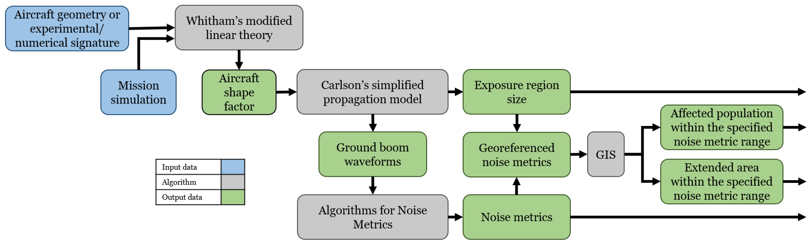
2. Surrogate Model for Sonic Boom Analysis

The proposed surrogate modeling framework aims to provide a fast and reliable estimation, inspired by AEDT software (version 3e), of sonic boom noise impacts. As illustrated in Figure 1, the model workflow is organized into four principal stages. In the first stage, input data comprising either explicit aircraft geometry (e.g., dimensions and shape) or numerical/experimental near-field pressure signatures need to be gathered. Essential operational parameters, such as the flight trajectory, speed, altitude, and aircraft weight, must also be collected. In the second stage, Whitham’s modified linear theory [28] is applied to compute the characteristic N-waves and associated aircraft shape factors. In the third stage, atmospheric propagation is conducted accounting for standard stratified pressure and temperature profiles. Specifically, Carlson’s propagation model [21] is used to integrate the shape factors to simulate ground level waveforms. To capture the influence of rise time on human annoyance, established empirical correlation is adopted [22,23]. In the final stage, each ground level waveform undergoes spectral and time domain processing, including fast Fourier transform (FFT), zero padding, and windowing, to compute standard sonic boom metrics. These metrics are then georeferenced and overlaid on population density maps within a GIS environment, yielding both noise contour visualizations and quantitative exposure statistics. Detailed descriptions of each module follow in subsequent sections.
The case study analyzed involves a Mach 2 aircraft [29]. This aircraft, referred to as the CS1a (Figure 2), was conceived as part of the EU-funded MOREandLESS project [7].
Two operational scenarios were considered for the CS1a. The first scenario involves a long-haul flight compatible with the aircraft’s maximum range, focusing solely on ground level noise metrics. The second scenario considers a simple overland flight to estimate both the number of people impacted and the extent of areas affected by varying ranges of noise metrics. In the first scenario, the selected route starts from Milan Malpensa Airport (MXP) and lands in New York John F. Kennedy International Airport (JFK). Otherwise, the overland scenario simulates the CS1a cruising over Italy.

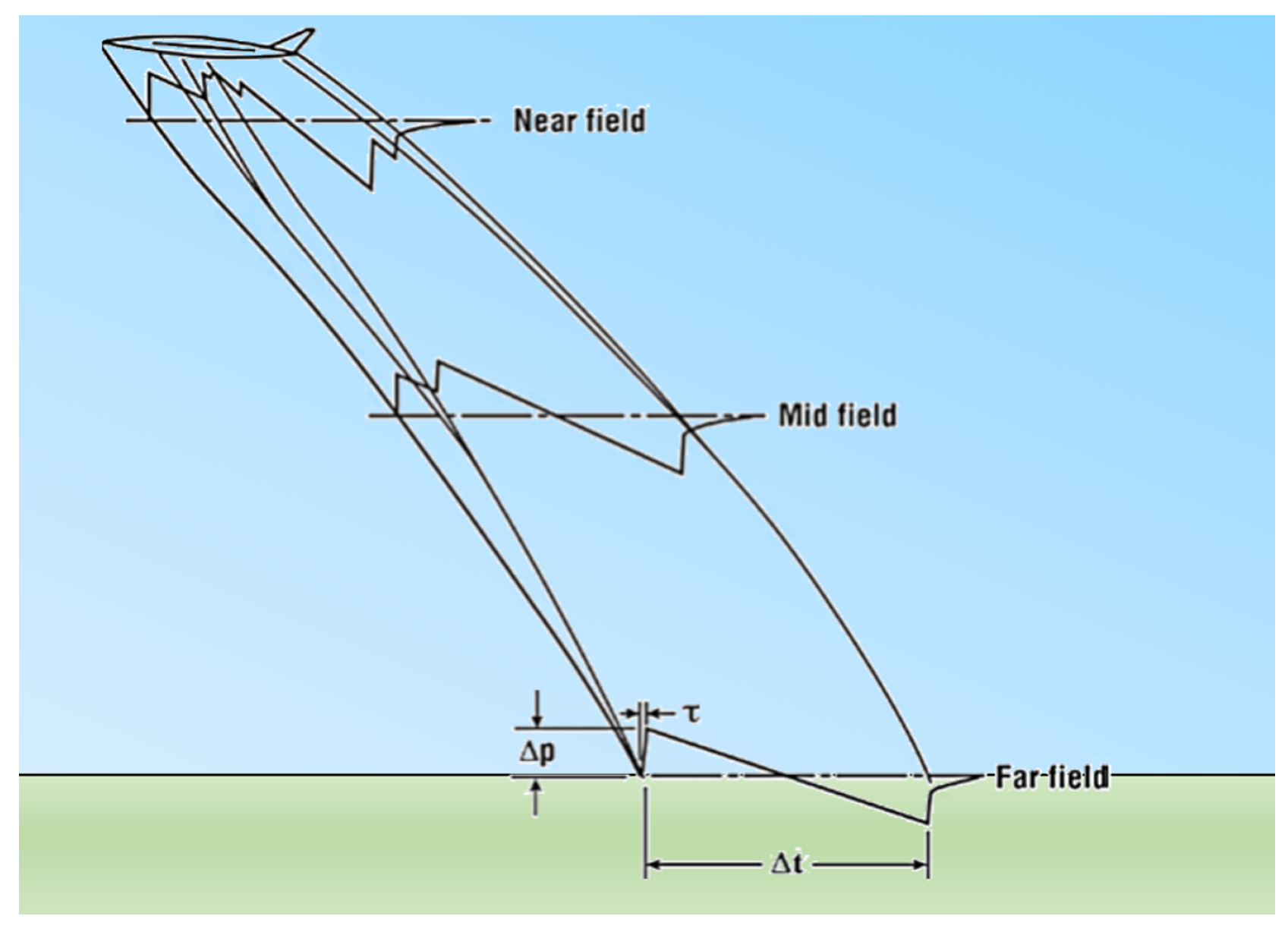
2.1. Near-Field Pressure Signatures

Computational fluid dynamics (CFD) techniques were employed to investigate the flow around the CS1a aircraft, addressing the strong non-linearities and three-dimensional interactions near the fuselage. Specifically, earlier work conducted within the MOREandLESS project provided near-field acoustic signatures at three distinct mission points (Table 1), each of which were evaluated across various azimuth angles [30].
Numerical simulations were performed with the open-source SU2 multiphysics suite (version 7.2.0) [31]. An Euler approach was applied, without activating turbulence models, for the near-field sonic boom analysis. The HLLC numerical scheme was adopted, and the gradients were calculated using the Green Gauss method. A detailed description of the computational set-up adopted for the CS1a benchmark is provided by [30].
Figure 3 defines the azimuth angle ϕ and shows the resulting near-field pressure signatures for the three mission points. The azimuth was measured clockwise about the aircraft centerline as viewed by the reader, with ϕ = 0° directly beneath the fuselage and increasing toward the starboard side.
Predicted pressure signatures were extracted on a cylindrical surface located at H / L = 3 , where H is the perpendicular distance from the vehicle, and L is its overall length. The simulations captured a distinct N-wave, which was preceded by a small pressure rise produced by the interaction between the nose-generated and wing-induced shock waves. Between ϕ = 0° and 60°, the progressive distortion of the N-wave highlighted the growing influence of the wing in the starboard quadrant.

2.2. Whitham’s Modified Linear Theory

When an object moves through the air at supersonic speeds, it generates a system of shock waves whose characteristics depend on its geometry. For simple, axisymmetric bodies (e.g., projectiles), the shock wave system typically comprises a bow shock at the front and a tail shock at the rear. In contrast, complex geometries, such as those of aircraft, produce multiple shock waves that, at large distances, typically coalesce to form an N-wave signature (Figure 4). This N-wave is characterized by a rapid compression at the bow shock, which is followed by a decompression below atmospheric pressure, and then recompression at the tail shock, which, when combined, results in a sonic boom [32].
Whitham’s linear theory posits that, for homogeneous, inviscid, and supersonic flows, as well as for slender, smooth bodies observed from a sufficient distance, the flow perturbations can be expressed as integrals of the source distribution [28]:
F ( y ) = 1 2 π 0 y A ( ξ ) y ξ d ξ ,
where A represents the total equivalent area distribution, accounting for both the volume term (the physical cross-sectional area calculated at the Mach angle) and the lift term (the cumulative lift in units of area). Here, A ( ξ ) is the second derivative of A with respect to the longitudinal coordinate ξ . In addition, y is the characteristic coordinate measured along the aircraft axis, and the integration extends from the nose ( ξ = 0 ) to the station at y.
The corresponding first-order pressure increment is as follows:
Δ p = p γ M 2 2 β r F ( y ) ,
where p is the freestream static pressure, γ the air specific heat ratio (typically 1.40 for air), M the freestream Mach number, β the Prandtl Glauert compressibility factor ( M 2 1 ), and r the radial distance from the source. Equation (2) offers a convenient first approximation to the sonic boom pressure signature, but the small perturbation assumption precludes an exact prediction of shock locations. To address this limitation, Whitham extended the formulation with a nonlinear correction that accounts for the local flow properties variations:
y t = y k r F ( y ) ,
where
k = ( γ + 1 ) M 4 2 β 3 .
In this study, the Whitham F-functions were determined by extrapolating the near-field pressure data obtained from CFD analysis to a reference distance r 0 using Equations (2) and (3):
F ( y ) = Δ p p 2 β r 0 γ M 2 ,
y = y t ( r 0 ) + k r 0 F ( y ) .
The pressure signature at any arbitrary distance r was then determined by substituting Equation (5) into Equation (2). When the function becomes multivalued, discontinuities (shocks) were introduced to satisfy the equal area rule.

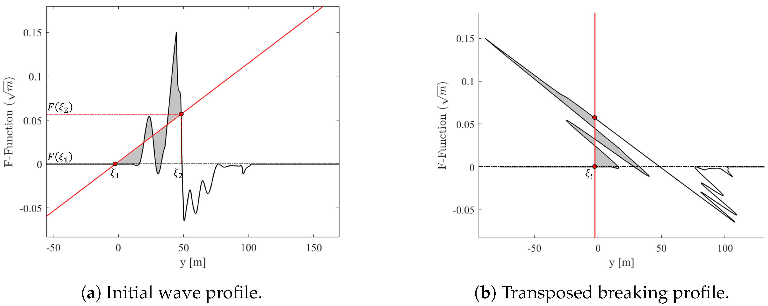
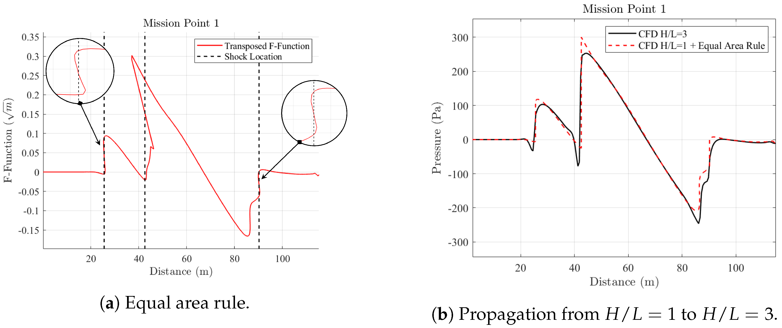
Whitham’s Equal Area Rule

The pressure signal propagates at the local speed of sound, with each point of the signal advancing in accordance with its amplitude. Consequently, higher pressure regions travel slightly faster than lower pressure regions, leading to wave distortion and, eventually, the development of multivalued regions. The physically unrealistic multiple pressure values are resolved through the formation of shocks [33]. Whitham’s method for determining shock locations, commonly known as the equal area rule, introduces an appropriate discontinuity that balances the areas above and below the shock line, ensuring conservation across the wave and implying that the shock velocity equals the average of the characteristic velocities on either side [34]. This approach is particularly effective for sonic boom problems, where pressure variations are treated as weak disturbances:
1 2 F ( ξ 1 ) + F ( ξ 2 ) ( ξ 2 ξ 1 ) = ξ 1 ξ 2 F ( ξ ) d ξ ,
where F ( ξ ) represents the initial wave profile, ξ is the characteristic variable, and ξ 1 and ξ 2 are the values of ξ on the two sides of the shock (Figure 5). The left side of equation represents the area under the straight line (the shock) connecting F ( ξ 1 ) and F ( ξ 2 ) , while the right term is the actual area under the curve F ( ξ ) from ξ 1 and ξ 2 .

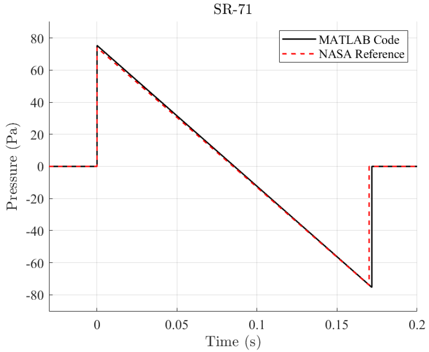
2.3. Propagation of Sonic Boom Signatures to Ground Level Through Homogeneous Atmosphere

Whitham’s modified linear theory does not account for atmospheric variations and is, therefore, only applicable to a homogeneous atmosphere. Under this limitation, the non-linear correction for local flow variations corresponds to the slope of the characteristic lines for area balancing, which is expressed as 1 / ( k r ) [28], where k is defined in Equation (4) and r is the radial distance from the source. To validate the Whitham procedure, the numerical near-field signature extracted from the CFD data at H / L = 1 was used as the input for the Whitham equal area rule code. The resulting waveform was then propagated to H / L = 3 (dashed red curve in Figure 6b) and compared with the CFD prediction at the same location (solid black line).
The comparison demonstrates good alignment between the propagated signature and the CFD results. The shock location is accurately predicted, although some dissipation of high-frequency content is observed in the CFD signature, likely due to the numerical dissipation from the computational scheme.
The near-field signatures for all three distinct mission points, each evaluated at various azimuth angles (see Figure 3), were then propagated to the ground. Figure 7 represents the resulting direct (thereby excluding any reflection factors) ground level sonic boom signatures, which were propagated through a homogeneous atmosphere.
As expected for conventional aircraft configurations, when the flow is sufficiently distant from the fuselage (typically beyond several hundred body diameters), the pressure signature evolves into a perfect N-wave. Under these far-field conditions, simplified analytical solutions for the shock strength Δ p and the duration Δ t can be derived [35]:
Δ p = 2 1 / 4 γ p M 2 1 1 / 8 γ + 1 1 / 2 0 y 0 F ( y ) d y r 3 / 4 ,
Δ t = 2 2 1 / 4 γ + 1 1 / 2 M a M 2 1 3 / 8 0 y 0 F ( y ) d y r 1 / 4 ,
where the decay law shifts from r 1 / 2 to r 3 / 4 and the F-function appears only in its integral form. Here, y 0 denotes the y value at which the integral of F ( y ) is maximized, and a represents the speed of sound. The N-wave equations can be further simplified by condensing the sonic boom characteristics as a single line on a parametric chart [21]. The principal factor governing the generation of the sonic boom, encompassing both the aircraft’s volume and lift distribution, can be mathematically expressed as follows:
K S = 2 1 / 4 γ γ + 1 1 / 2 0 y 0 F ( y ) d y L 3 / 4 .
By substituting K S into Equations (8) and (9), two expressions for the aircraft shape factor can be derived:
K S p = Δ p p ( M 2 1 ) 1 / 8 r 3 / 4 L 3 / 4 ,
K S t = Δ t M a γ 2 ( γ + 1 ) ( M 2 1 ) 3 / 8 r 1 / 4 L 3 / 4 .
For an ideal N-wave, as described by Whitham’s theory, both equations would yield the same K S value. In this study, the mean percentage error between K S p and K S t across all mission points and azimuth angles was only 1.3%. To avoid favoring one metric over the other, the arithmetic mean was adopted for each analyzed propagated signature:
K S = K S p + K S t 2 .
The results are presented in the following Figure 8 as a function of the azimuth angle for each mission point analyzed, with spline interpolations used to estimate the intermediate values for a smoother representation.

2.4. Propagation of Sonic Boom Signatures to Ground Level Through Standard Atmosphere

It is generally agreed that atmospheric conditions apply a strong influence on sonic boom propagation. Macro effects, such as pressure, temperature, and wind profiles, and especially their gradients, refract shock rays, redistributing the footprint on the ground and changing its intensity and lateral extent [33]. At smaller scales, turbulence, molecular absorption, and relaxation further reshape the waveforms, altering both shock strength and rise time. Since Whitham’s modified linear theory does not account for these mechanisms, an augmented distortion equation for the F-function is required to obtain accurate ground signatures, even when only the macro effects are retained [36]. Among the available approximations, Carlson’s simplified propagation method [21] offers an unrivaled balance between physical fidelity and computational efficiency for large-area environmental assessments conducted within far-field regions (under the assumption of a standard atmosphere). Contemporary ray-tracing solvers [16,17,18,19], which explicitly model nonlinear effects, atmospheric refraction, and attenuation, integrate the augmented Burgers equation on finely resolved atmospheric grids and, consequently, rely on extensive database of CFD near-field signatures for every parameter that can vary along the trajectory, like the Mach number, altitude, lift condition, and azimuth angle. Carlson condenses the entire vehicle influence into a single shape factor, K S , which is estimated from only a small set of representative CFD cases. The resulting closed-form expressions resolve each ray instantly, enabling full-trajectory, full-azimuth evaluations on continental scales, as well as permitting sensitivity analysis and regulatory studies. These outcomes, however, rest on several well-understood simplifications: a wind-less, standard atmosphere; straight and unaccelerated flight; the far-field N-wave assumption; and an assumed zero rise time. Extensive validation campaigns [21], nevertheless, confirm Carlson’s robustness under moderate departures from ISA, gentle maneuvers, and conventional configurations, with a conservative bias in predicted peak overpressure and duration. Rise time estimation, precluded by the discontinuous jumps inherent in linear weak-shock theory, can be approximated by folding attenuation mechanisms into the empirical 3 / Δ P rule [22,23], which yields the rise time (ms) as 3 divided by the shock overpressure (psf) (although without accounting for humidity effects). Within this framework, Carlson introduces amplification factors for overpressure and duration Equations (11) and (12), namely K P , K R , and K t , leading to the governing relations:
Δ P = K P K R K S p v p g ( M 2 1 ) 1 / 8 L 3 / 4 r e 3 / 4 ,
Δ t = K t K S γ + 1 γ M a v M 2 1 1 / 8 L 3 / 4 r e 1 / 4 ,
where K P scales the peak overpressure, K t adjusts the signature duration, and K R represents the reflection factor, which flight test data place in the interval 1.8–2.0 [21]. Treating K R as a constant is, however, a notable simplification: it ignores the terrain-induced phenomena, such as wavefront folding triggered by large slope variations, which can generate focal zones, caustics, and U-waves capable of markedly altering ground signatures [37,38]. Analogous modifications have been observed for urban canopies in simulations comparing boom propagation over built environments with the flat ground case [39,40,41]. A fully resolved treatment of these topographic and urban interactions is beyond the predictive scope of the present tool, so the constant K R assumption is retained as a pragmatic compromise consistent with the intended modeling fidelity. Moreover, for the urban scenarios, statistical analysis show that the median deviation of noise metrics from the flat ground baseline is approximately zero [39], indicating that the Carlson predictions could be interpreted as a representative mean solution. Unlike Whitham’s classical formulation, the static free-stream pressure adopted in Equation (14) is defined as the geometric average of the atmospheric pressure at the aircraft’s altitude, p v , and the atmospheric pressure at ground level, p g . Additionally, r e denotes the effective altitude, and a v is the speed of sound at the aircraft’s altitude.
Figure 9 illustrates the implementation of Carlson’s method. For validation, the SR-71 Blackbird was selected as a test case using the flight parameters and the shape factor provided in Carlson’s original work [21].
Following validation of the propagation model, the flight parameters listed in Table 1 and the shape factor derived in the previous section, as shown in Figure 8, were used to compute the CS1a ground signatures under standard atmosphere conditions (Figure 10). A reflection coefficient of 1.9 was applied. Ground altitudes along the flight path were retrieved from the Open-Elevation API and, for simplicity, the altitude directly beneath the aircraft was assumed to be equal to that at the point where the acoustic ray intersects the ground (see the left image in Figure 11). An iterative procedure that forced the two elevations to coincide exactly (right image in Figure 11) revealed negligible differences, which is an expected outcome given that the mismatch, of an order of a few hundred meters, is small relative to the several kilometers flight altitude and, therefore, has no discernible effect on the amplitude or duration of the predicted N-waves. It should be noted that the ground elevation variation along the flight path was included solely to capture the geometric spreading more accurately than a constant ground altitude assumption would allow. As reported in a previous section, detailed topographic effects are beyond the current tool’s scope. For the same reason, the ground on-track elevation profile was extended unchanged to ground off-track locations.
Notably, the rays generated at azimuth angles of 50 and 60 degrees during Mission Points 1 and 2 failed to reach the ground due to refraction effects. In contrast, the ray produced at 50 degrees during Mission Point 3 reached the ground. This discrepancy was attributed to the aircraft’s higher speed at Mission Point 3, which produces a sharper Mach cone and, therefore, a more perpendicular ray trajectory relative to the ground.

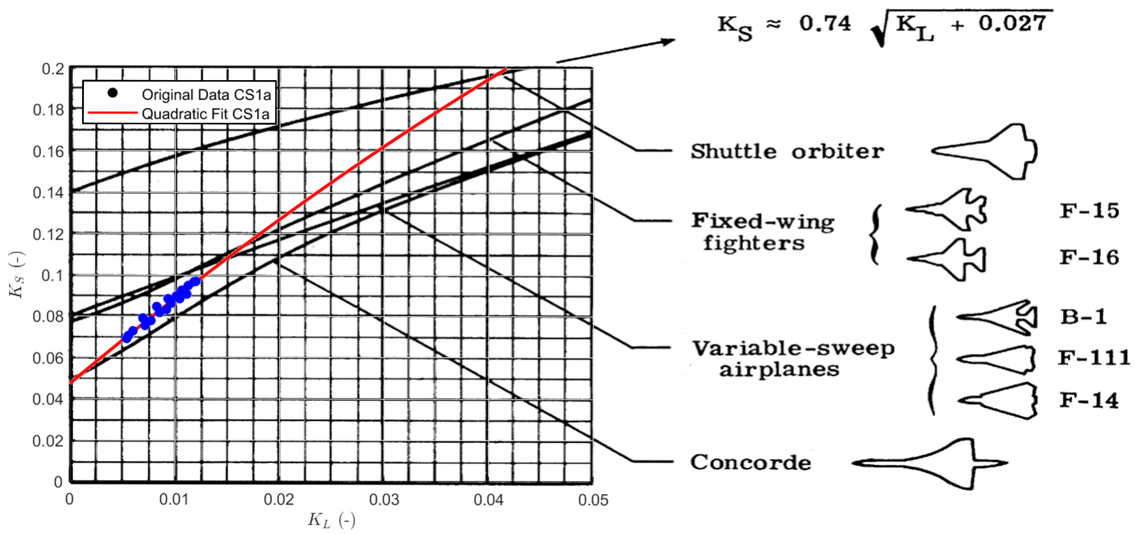
2.5. Aircraft Shape Factor and Mission Profile Regression Model

A comprehensive set of tests conducted across a wide range of operating conditions enabled the formulation of a generalized aircraft shape factor suitable for sonic boom prediction under generic flight conditions. A key step in this process was identifying the aircraft lift parameter K L :
K L = β W cos ( ϕ ) cos ( α ) 1.4 p v M 2 L 2 ,
where W denotes the aircraft weight. A second-order regression was performed, minimizing the root mean square error (RMSE) between the predicted and observed shape factors. Figure 12 compares the resulting CS1a regression curve with the aircraft shape factors derived from both historical sonic boom flight test programs and more contemporary aircraft [21].
It is important to highlight that the CS1a shape factor exhibits higher consistency and accuracy in regions closer to the regression points. Conversely, the lack of data points at large K L values necessarily limits the reliability of extrapolated predictions. This shortcoming has little practical impact, as the nominal CS1a operating envelope lies squarely within the data-rich portion of the K L domain. Additional confidence in the fit arises from the geometric kinship between the CS1a and the Concorde. In the limiting case K L = 0 , where only volume contribution is present, the CS1a shape factor converges to that of the Concorde. Moreover, because the two aircraft share comparable weight, cruise Mach number, length, and cruise altitude, the CS1a is expected to produce a cruise phase sonic boom annoyance only marginally greater than that historically associated with the Concorde.
Based on the second-order polynomial regression representing the CS1a shape factor, the following equation will be used in the subsequent analyses to simulate the sonic boom produced and its associated annoyance during a transatlantic route:
K S = 14.3067 K L 2 + 4.2628 K L + 0.0474 .

3. Results of the Presented Procedure on Sonic Boom Impact

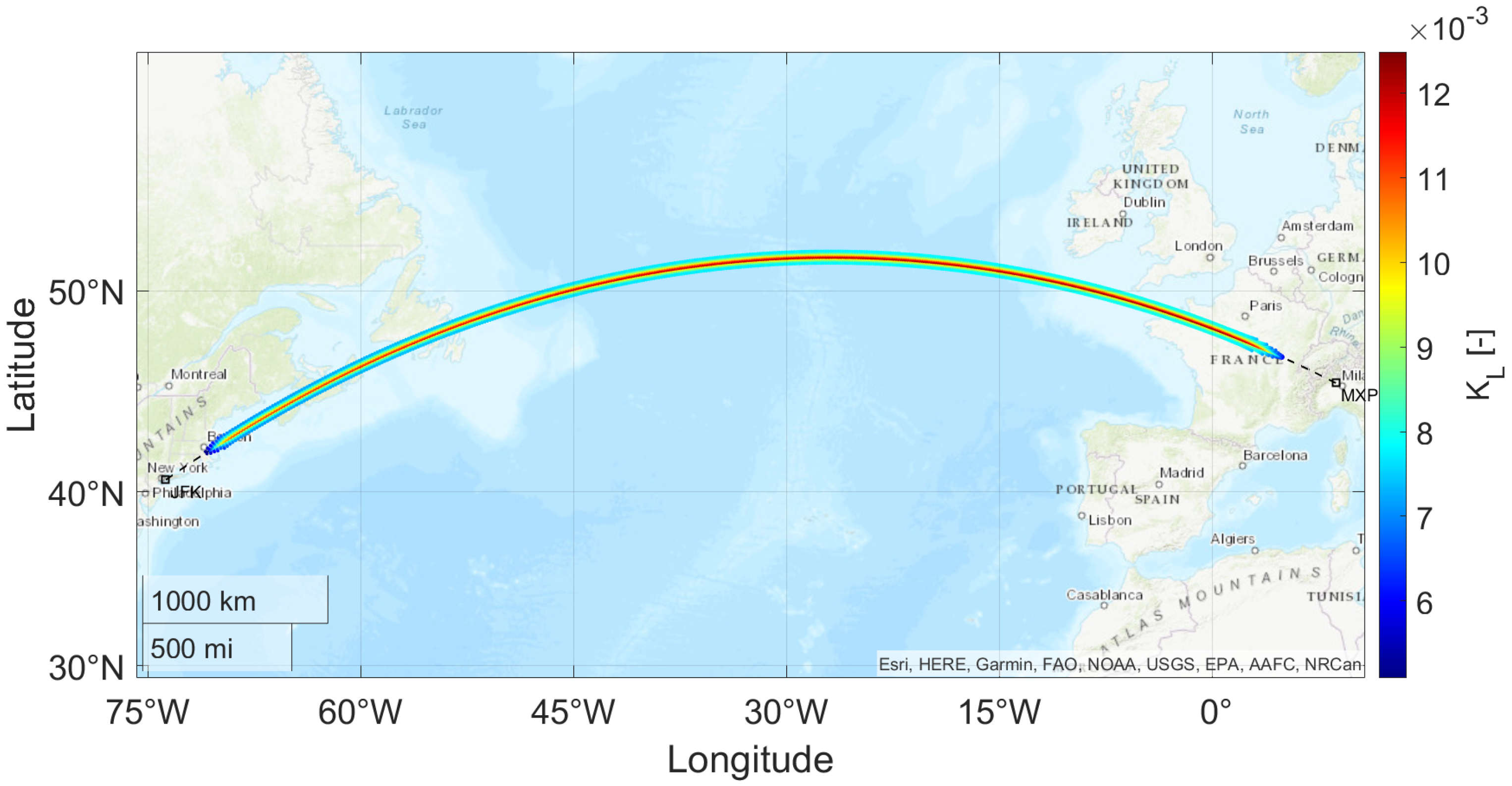
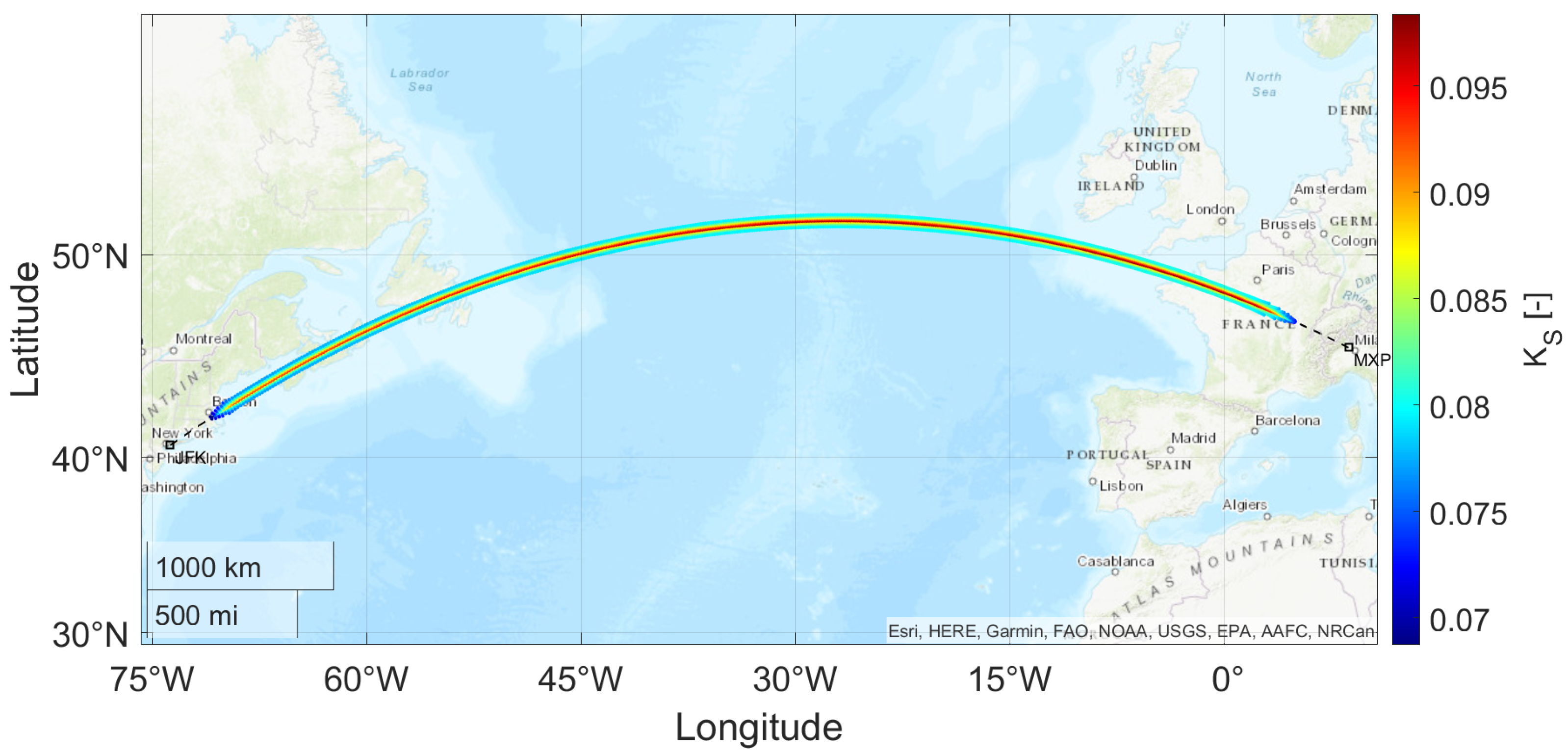
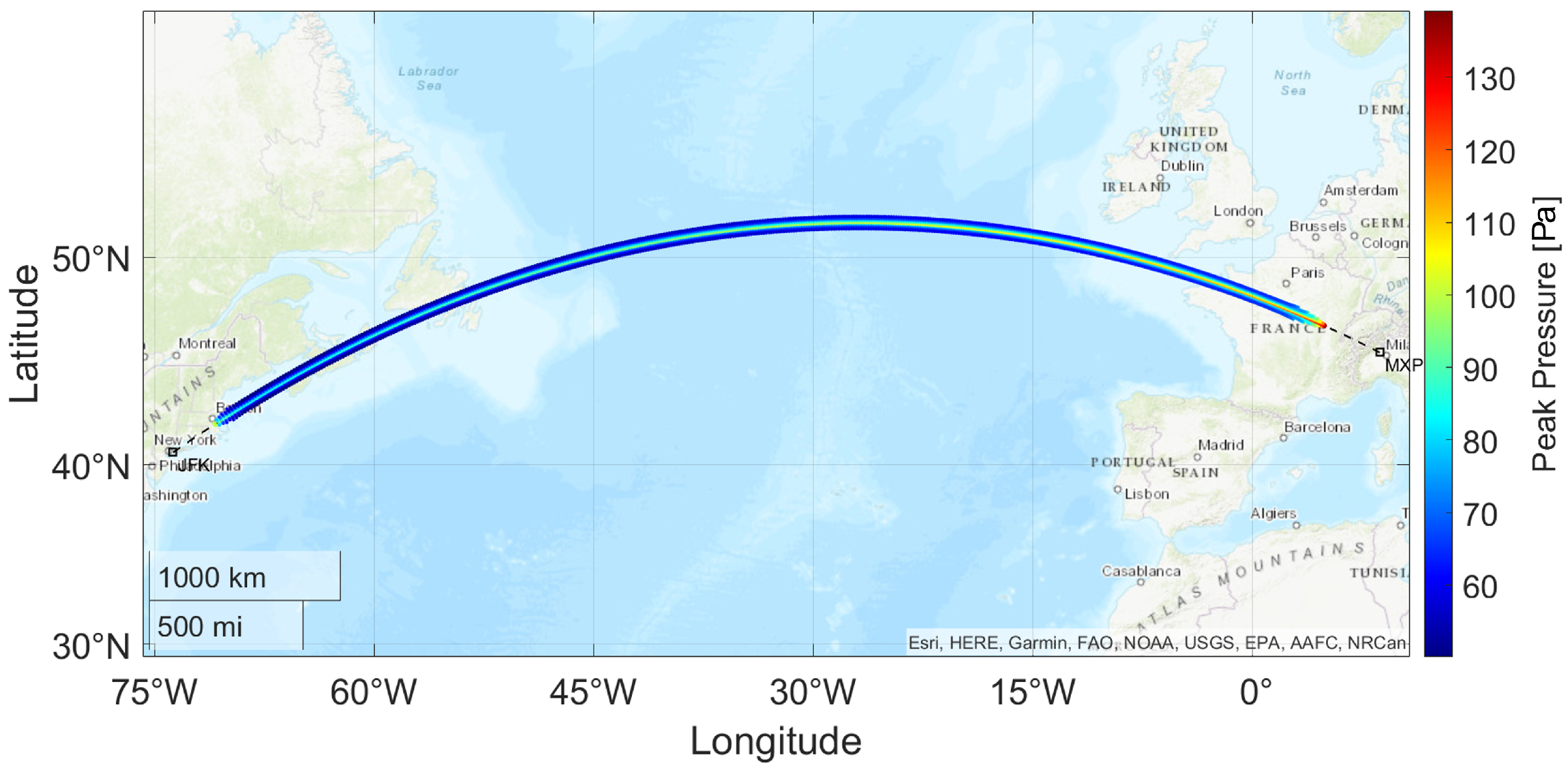
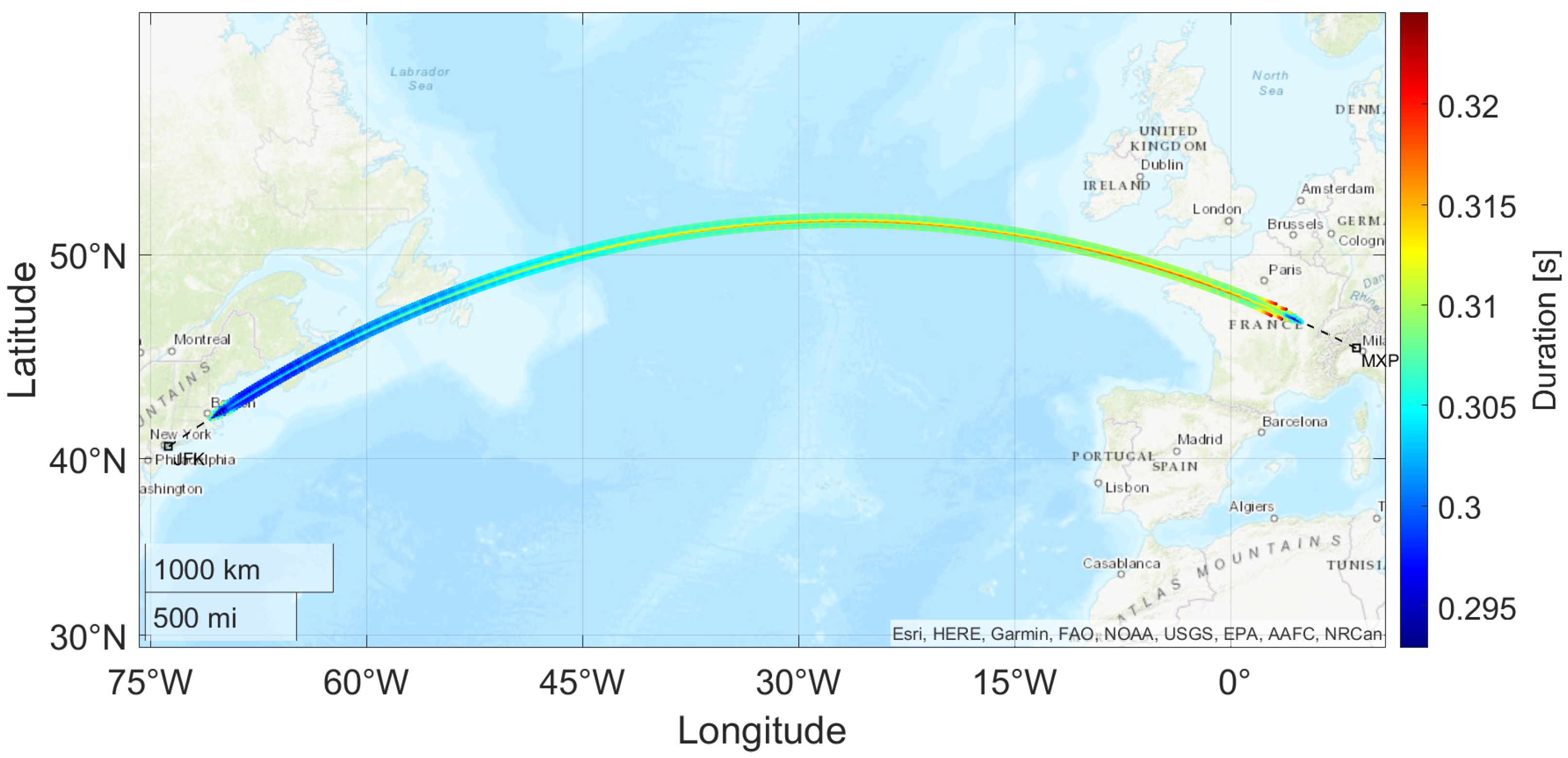
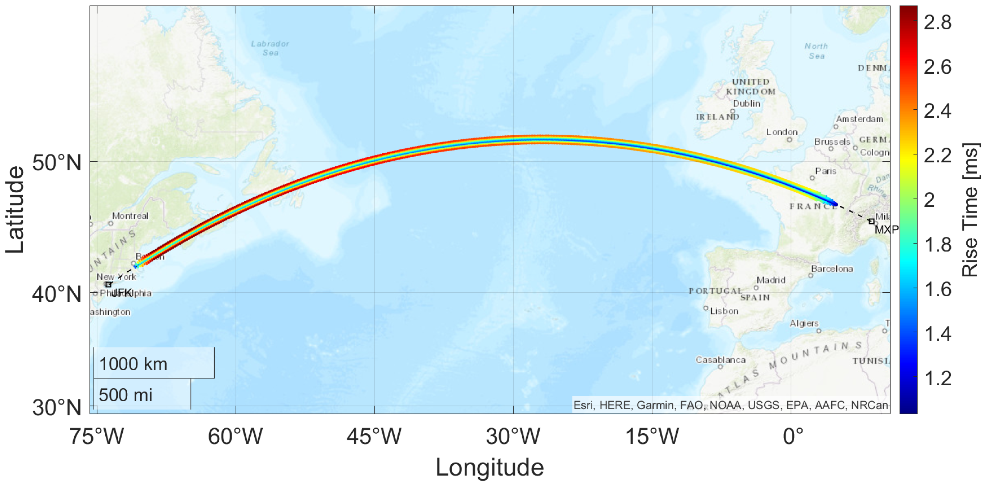
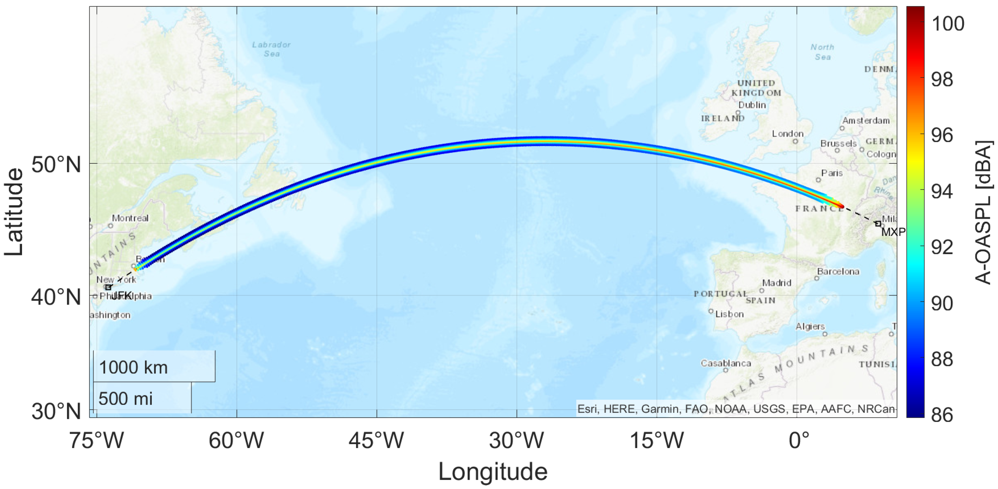
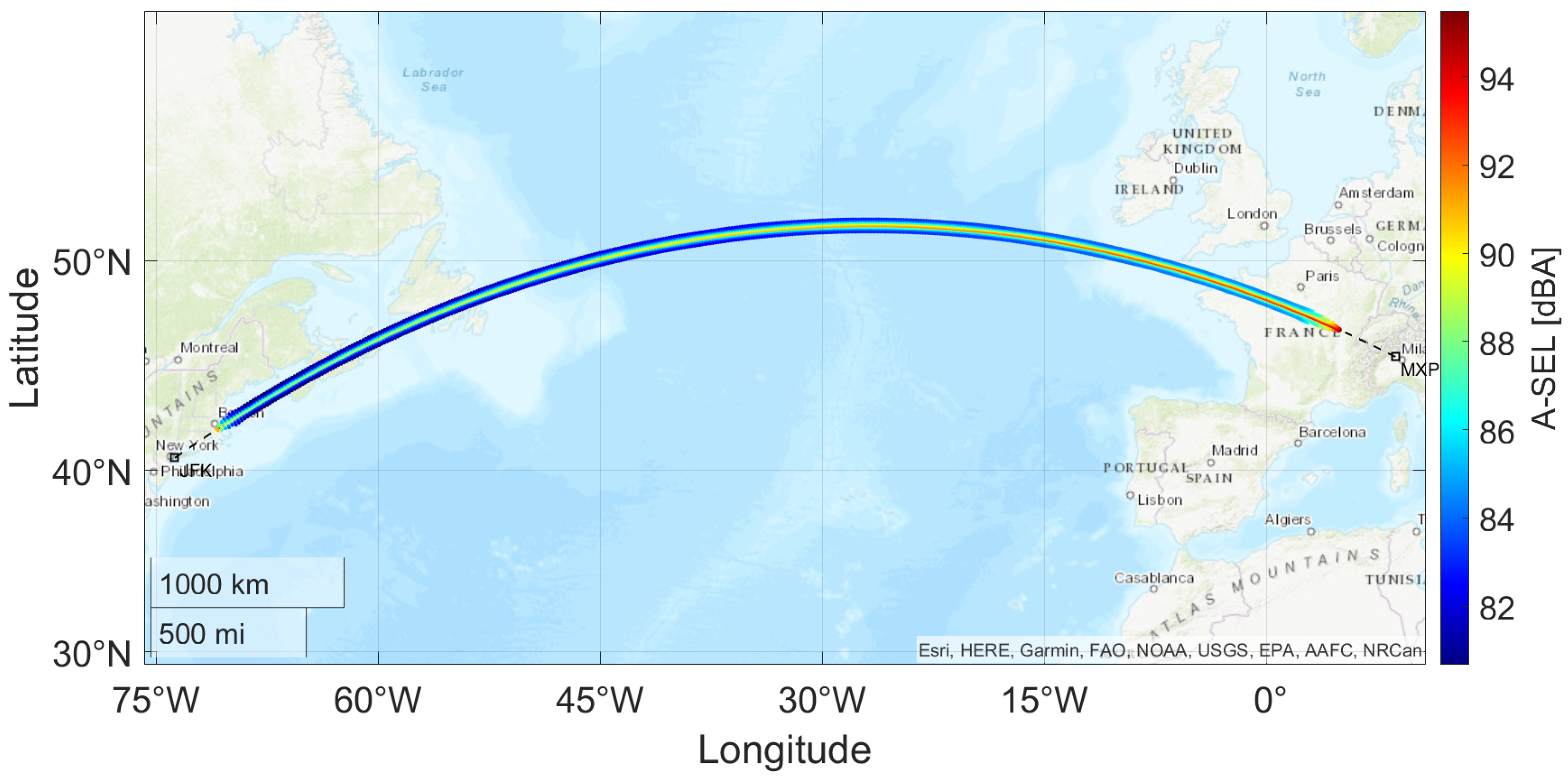
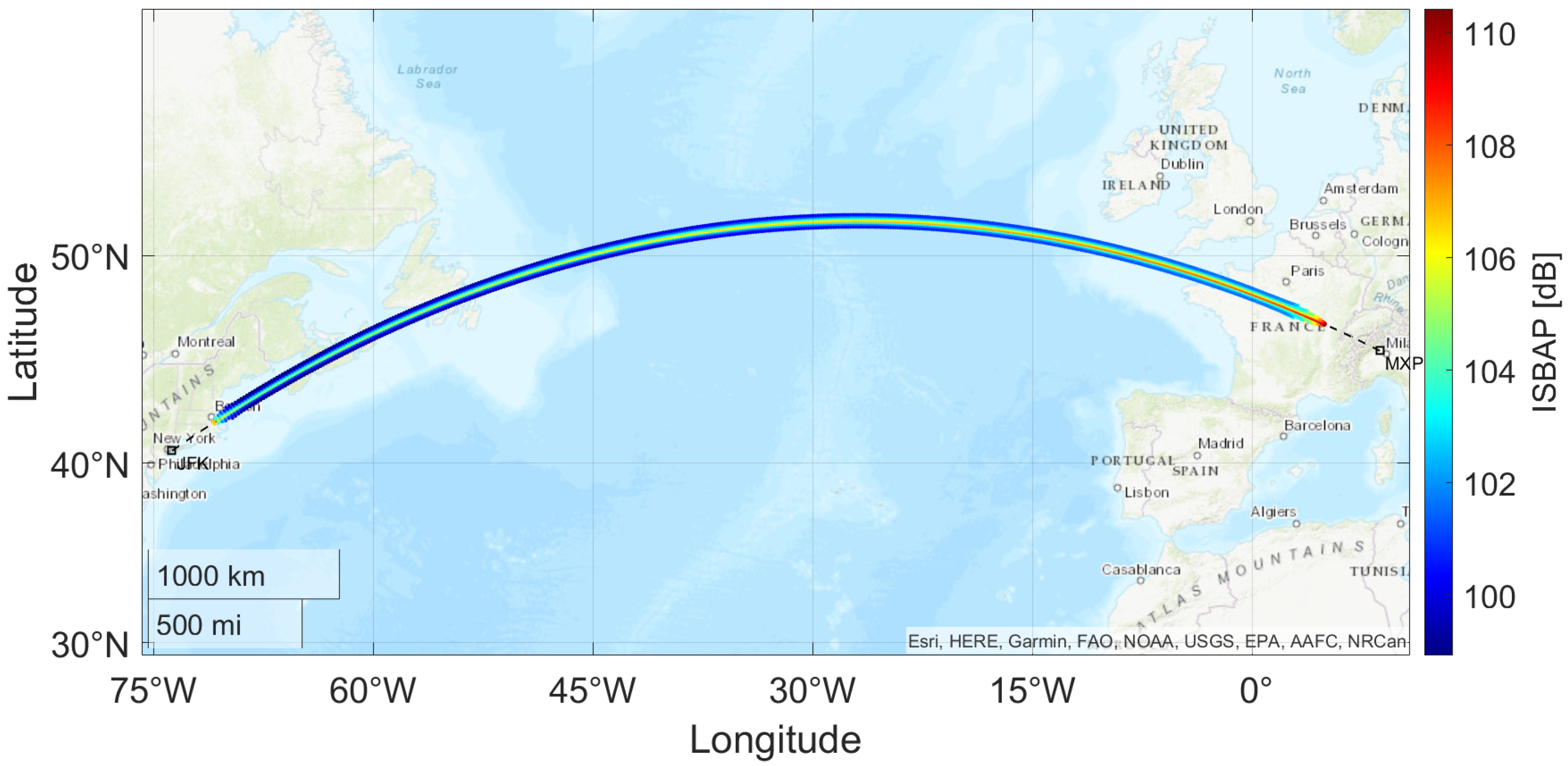
3.1. Transatlantic Route Impact Assessment: Milan to New York Case Study

The annoyance caused by noise is a complex topic, and sonic booms pose unique challenges due to their low-frequency energy and transient nature. Unlike conventional noise, it requires specialized metrics to effectively characterize both outdoor and indoor annoyance. Extensive laboratory testing and data analysis have identified a well-suited subset of metrics for predicting human responses [24]. These metrics are grouped into three distinct categories:
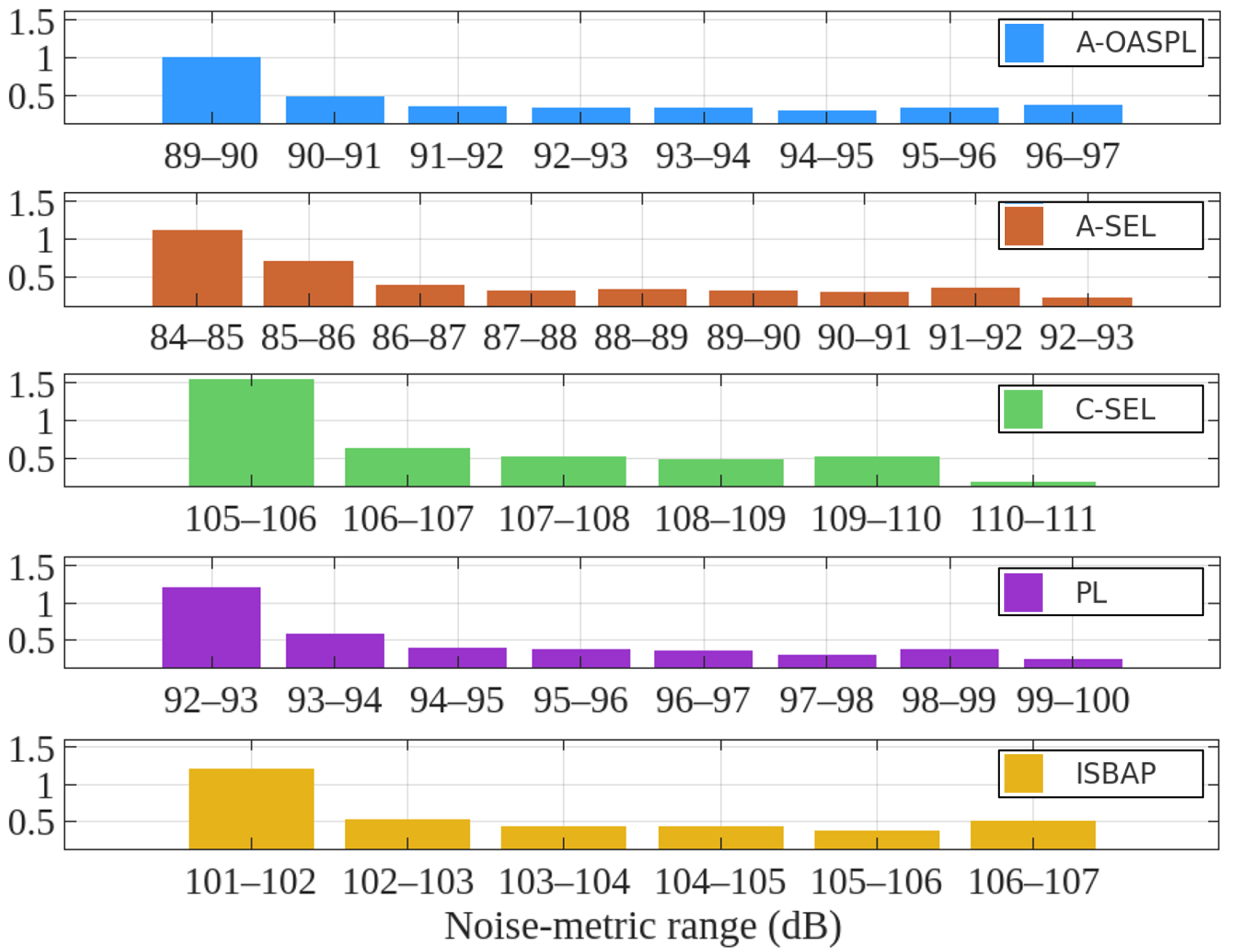
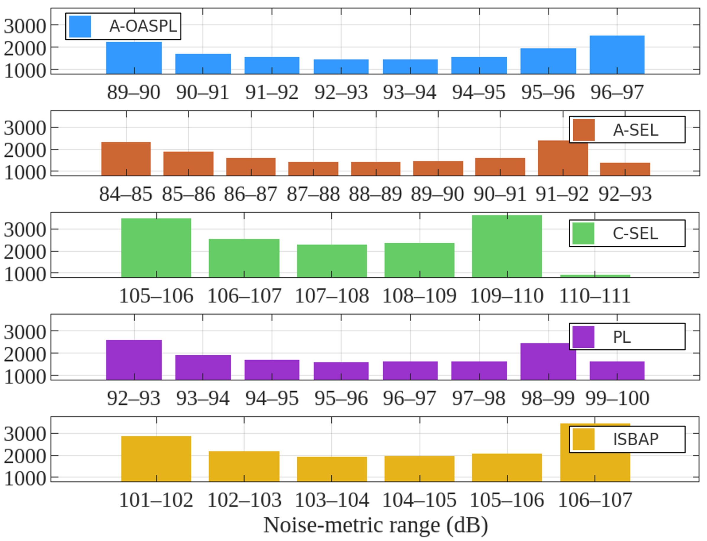
  • Engineering metrics, which quantify physical sound characteristics;
  • Loudness metrics, which account for human perception of sound;
  • Hybrid metrics, which integrate multiple metrics to provide a comprehensive sonic boom assessment.
In this study, the selected metrics are as follows:
  • The A-weighted Overall Sound Pressure Level (A-OASPL) [42] and the A- and C-weighted Sound Exposure Levels (SEL) [43];
  • The Perceived Level (PL) in decibels, which is calculated based on Stevens’ Mark VII equal loudness contours [44,45];
  • The Indoor Sonic Boom Annoyance Predictor (ISBAP), which evaluates indoor annoyance using solely external measurements [46,47].
The Sound Pressure Level (SPL), which forms the basis for the computation of the noise metrics, is mathematically expressed as follows:
S P L = 10 log 10 P S D Δ f p r e f 2 ,
where P S D represents the power spectral density of the signal, Δ f is the frequency resolution, and p r e f is the reference pressure (20 μPa), corresponding to the threshold of human hearing. Specifically, all N-waves were zero-padded to extend their total duration to 20 times their original length. Spectral estimates were then obtained with Welch’s method [48] using a single segment whose length exactly matched that of the zero-padded waveform. Consequently, the product P S D Δ f in the SPL formula literally equals the energy contained in each discrete frequency bin.
To simulate a long-haul flight, the mission profile [49], corresponding to an effective range of 6500 km, was utilized. The selected route, from Milan Malpensa (MXP) to New York John F. Kennedy International Airport (JFK), is illustrated in Figure 13, which details key input parameters, such as the flight altitude, Mach number, flight path angle, and lift (which was assumed to be equal to the weight for a trimmed vehicle).
Figure 14 and Figure 15 present contour plots of the CS1a shape factor and lift parameter along the MXP-JFK route. Their spatial distributions are interpretable by referring to the corresponding governing equations detailed earlier. The computed shape factor was then used to generate the N-wave signatures along the flight path, and these signatures were post-processed to extract the relevant noise metrics.
The remaining figures provide a comprehensive overview of the key acoustic parameters associated with the N-waves along the flight path. Figure 16 illustrates the acoustic peak pressure of the N-waves, and this is followed by Figure 17, which shows the duration of the N-waves. Figure 18 depicts the variation in rise time. Figure 19 provides the A-weighted Overall Sound Pressure Level (A-OASPL), while Figure 20 and Figure 21 display the A-weighted and C-weighted Sound Exposure Levels (A-SEL and C-SEL), respectively. Additionally, Figure 22 depicts the Perceived Loudness (PL), and Figure 23 concludes with the Indoor Sonic Boom Annoyance Predictor (ISBAP).
Figure 16 highlights that the peak pressure is maximized along the aircraft’s ground track and decreases in the perpendicular direction. This behavior occurs because rays at higher azimuth angles travel longer distances and are associated with lower K S values (only a fraction of the total lift is transferred to the ground in these directions). Furthermore, as the aircraft ascends and burns fuel during flight, two other effects are observed:
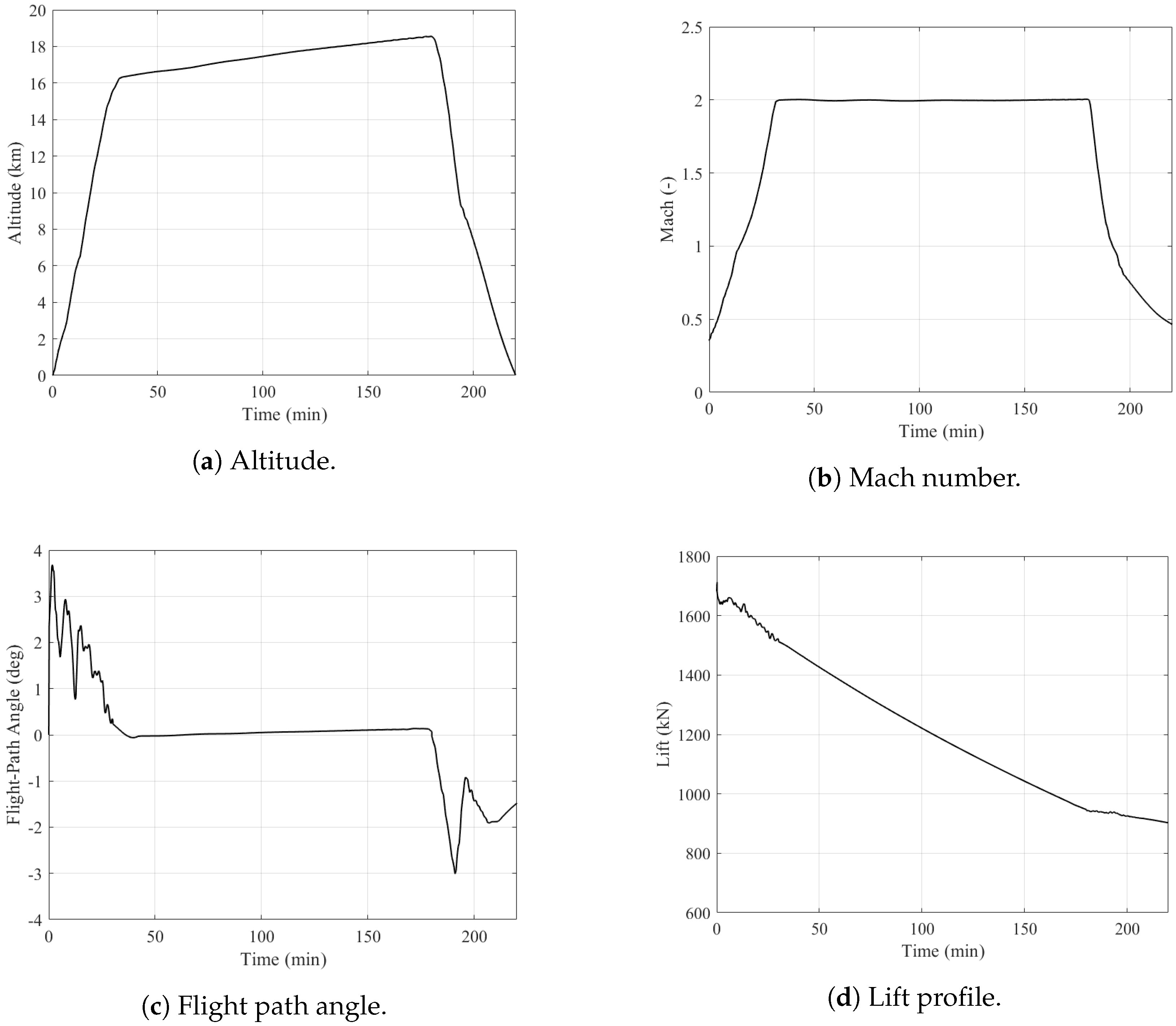
  • The increasing altitude causes the rays to cover a greater distance, reducing the sonic boom intensity;
  • Fuel burn results in a lighter aircraft, thereby lowering the lift requirement and further decreasing the peak pressure along the ground track.
Figure 16 also reveals that higher pressure values occur at both the beginning and end of the flight profile, corresponding to the lower altitudes during the supersonic climb and descent phases. In these phases, the sonic boom footprint is more confined compared to the broader carpet observed during cruise conditions.
It is important to note that these results are based on models that assume a stationary regime. In practical scenarios, any rapid deviation from steady, level supersonic flight can significantly alter the location, number, and intensity of the ground shock wave patterns. In this study, the flight profile was approximated by a series of multiple stationary states, which provided a simplified framework for the analysis.
The duration behavior illustrated in Figure 17 was considerably more uniform than the peak pressure due to the balancing effects of certain parameters in the signature formation process. For instance, while the Whitham equations predicted that the duration should increase in the direction normal to the flight path, owing to longer ray paths, the decrease in the shape factor at higher azimuth angles counteracted this increase, resulting in a reduced duration. Furthermore, the signature duration factor introduced by Carlson to account for standard atmospheric conditions also played a significant role in modulating the duration. This interplay is clearly observable in the ground signatures presented above, which were computed for both homogeneous (Figure 7) and standard atmospheres (Figure 10) across the three mission points and various azimuth propagation directions. Finally, along the aircraft’s ground track, the dominant influence of K S resulted in a decreasing trend in duration.
Overall, the noise metrics reported in this paper exhibited a similar trend, decreasing both along and perpendicular to the aircraft’s ground track.
Given the considerable spatial extent of the sonic boom carpet, the following section will assess the potential impact by estimating the number of people affected in a hypothetical supersonic overflight.

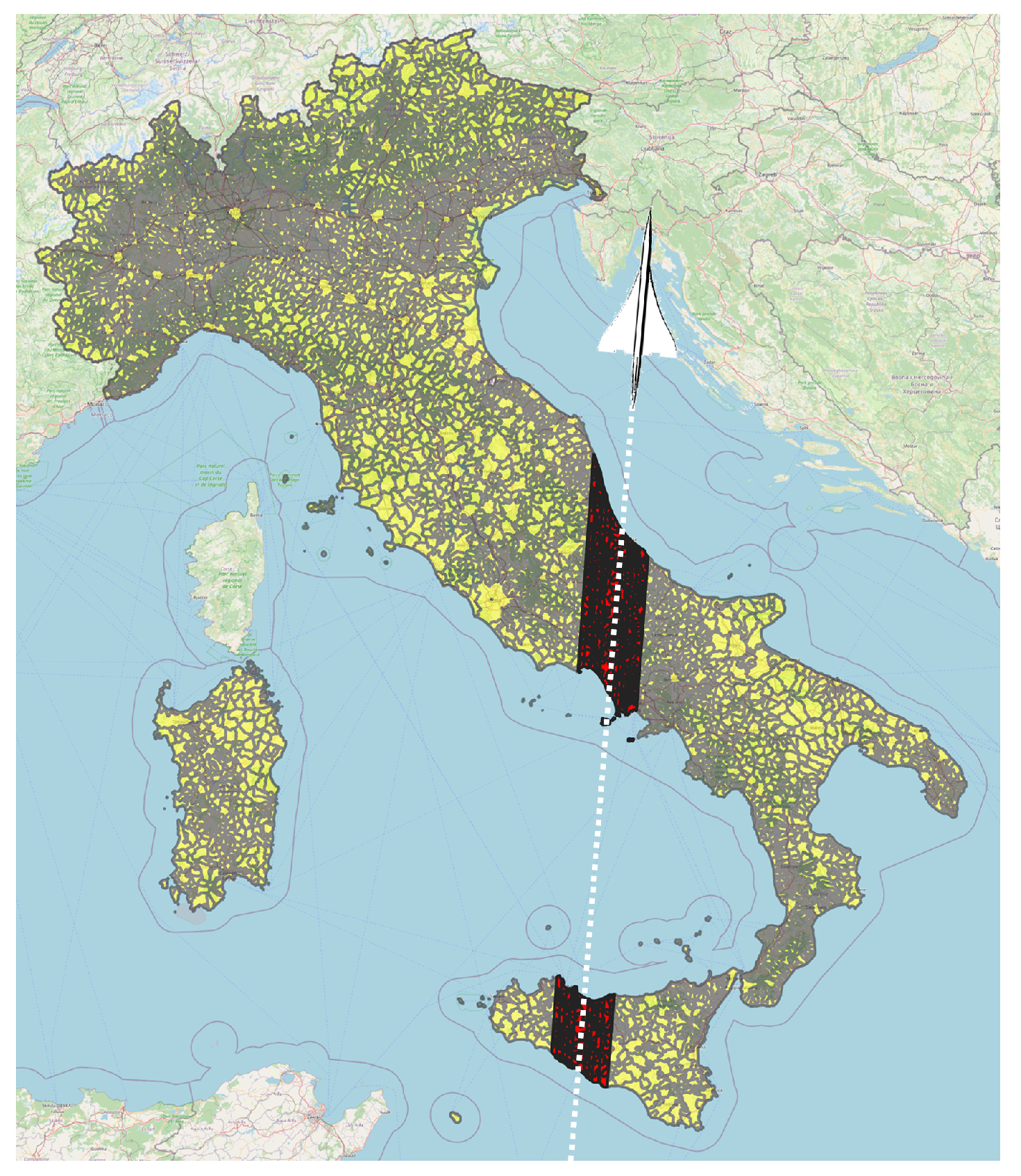
3.2. Supersonic Flight Impact over Italy

In a second scenario, the CS1a was simulated during a simple overflight of Italy under cruise conditions. The flight parameters, summarized in Table 2, were assumed to remain constant throughout the entire route. This scenario was specifically designed to estimate the number of people impacted by the sonic boom, as well as the extent of the affected areas across various regions in Italy.
Using these parameters, the sonic boom carpet’s extent was calculated and overlaid onto a map of Italy. Specifically, Figure 24 highlights the regions affected by the sonic boom (red areas).
Figure 25 presents a bar graph of the population (in millions) affected by sonic booms, and these were categorized by noise metric ranges across five distinct metrics (A-OASPL, A-SEL, C-SEL, PL, and ISBAP). Each metric was divided into noise ranges of 1 dB increments. In parallel, Figure 26 illustrates the impacted area (in square kilometers) for the same noise metric ranges.
The analysis indicates that about 4 million people in Italy could be exposed to varying levels of sonic boom annoyance (Figure 25). Given Italy’s total population of approximately 60 million, this suggests that around 6.7% of the population might be impacted by a supersonic flight. Naturally, this number is variable as it depends on both the flight trajectory and the spatial distribution of population density.
Regarding the affected area, the analysis estimates that over 15,000 km2 of Italy was exposed to the CS1a sonic boom (Figure 26), which represents roughly 4.7% of Italy’s total area (320,000 km²).

4. Conclusions

This work highlights the growing need for an efficient, comprehensive framework to quantify the environmental impact of sonic booms, particularly given the rising interest in supersonic commercial flight. By coupling Whitham’s modified linear theory and Carlson’s simplified propagation model, the proposed tool balances physical fidelity and computational speed, enabling rapid sensitivity analyses and potentially supporting regulatory assessments. The framework predicts ground level sonic boom signatures, derives outdoor and indoor annoyance metrics, and maps both the number of people impacted and the geographical extent of exposure.
The tool’s capabilities were demonstrated through two case studies: a long-haul flight from Milan to New York and a supersonic overflight of Italy. For the Italian scenario, the model predicts that roughly four million people, about 6.7% of the country’s 60 million residents, could be exposed to varying levels of sonic boom annoyance. Moreover, the impacted area could exceed 15,000 km2, or 4.7%, of Italy’s total area.
These findings rest on several well-understood simplifications: a windless standard atmosphere, straight and unaccelerated flight, the far-field N-wave assumption, and zero rise time (with rise time subsequently estimated from an empirical correlation). While an N-wave remains an appropriate approximation for contemporary supersonic aircraft, future evaluations, particularly of low-boom configurations, may require waveform specific refinements or, at minimum, the use of the present tool as a conservative estimator of peak pressure and duration alone. In addition, extending the framework to cumulative noise metrics will be essential for evaluating repeated operations over the same communities.
Overall, the proposed tool provides a robust foundation for decision making in supersonic flight management and environmental policy.

Author Contributions

Conceptualization, G.F.; methodology, G.F. and F.P.; software, G.F. and A.G.; validation, G.F., A.G., and M.B.; formal analysis, L.F.; investigation, G.F.; resources, M.B. and L.F.; writing—original draft preparation, G.F.; writing—review and editing, F.P.; supervision, L.F.; project administration, M.B. All authors have read and agreed to the published version of the manuscript.

Funding

This research received no external funding.

Data Availability Statement

The raw data supporting the conclusions of this article will be made available by the authors on request.

Conflicts of Interest

The authors declare no conflicts of interest.

Abbreviations

The following abbreviations are used in this manuscript:
dBDecibel
PLdBPerceived level of noise in decibel
FAAFederal Aviation Administration
ICAOInternational Civil Aviation Organization
CAEPICAO’s Committee on Aviation Environmental Protection
AEDTAviation Environmental Tools Suite
CFDComputational fluid dynamics
SPLSound pressure level
SELSound exposure level
PSDPower spectral density
ISBAPIndoor Sonic Boom Annoyance Predictor
DNLDay–Night Average Sound Level
FFTFast Fourier transform
OASPLOverall Sound Pressure Level
MXPMilan Malpensa Airport
JFKNew York John F. Kennedy International Airport

References

  1. Bonavolontà, G.; Lawson, C.; Riaz, A. Review of sonic boom prediction and reduction methods for next generation of supersonic aircraft. Aerospace 2023, 10, 917. [Google Scholar] [CrossRef]
  2. Pawlowski, J.; Graham, D.; Boccadoro, C.; Coen, P.; Maglieri, D. Origins and overview of the shaped sonic boom demonstration program. In Proceedings of the 43rd AIAA Aerospace Sciences Meeting and Exhibit, Reno, NV, USA, 10–13 January 2005; p. 5. Available online: https://ntrs.nasa.gov/citations/20050165091 (accessed on 27 December 2024).
  3. Cowart, R.; Grindle, T. An overview of the Gulfstream/NASA Quiet SpikeTM flight test program. In Proceedings of the 46th AIAA Aerospace Sciences Meeting and Exhibit, Reno, NV, USA, 7–10 January 2008; p. 123. [Google Scholar]
  4. Honda, M.; Yoshida, K. D-SEND project for low sonic boom design technology. In Proceedings of the 28th International Congress of the Aeronautical Sciences, Brisbane, Australia, 23–28 September 2012; pp. 1–8. [Google Scholar]
  5. CORDIS. Environmentally Friendly High Speed Aircraft. Available online: https://cordis.europa.eu/project/id/516132 (accessed on 27 December 2024).
  6. CORDIS. (LTO) noiSe and EmissioNs of supErsoniC Aircraft. Available online: https://cordis.europa.eu/project/id/101006742 (accessed on 27 December 2024).
  7. CORDIS. MDO and REgulations for Low-Boom and Environmentally Sustainable Supersonic Aviation. Available online: https://cordis.europa.eu/project/id/101006856 (accessed on 27 December 2024).
  8. NASA. Quesst Mission Overview. Available online: https://www.nasa.gov/mission/quesst/ (accessed on 27 December 2024).
  9. Lockheed Martin. X-59 Quiet Supersonic Technology (QueSST) Product Card. Available online: https://www.lockheedmartin.com/content/dam/lockheed-martin/aero/documents/Product%20Card%20X-59.pdf (accessed on 27 December 2024).
  10. Doebler, W.J.; Wilson, S.R.; Loubeau, A.; Sparrow, V.W. Simulation and regression modeling of NASA’s X-59 low-boom carpets across America. J. Aircr. 2023, 60, 509–520. [Google Scholar] [CrossRef]
  11. Morgenstern, J.; Buonanno, M.; Norstrud, N. N+2 Low Boom Wind Tunnel Model Design and Validation. In Proceedings of the 30th AIAA Applied Aerodynamics Conference, New Orleans, LO, USA, 25–28 June 2012; Volume 3217. [Google Scholar]
  12. Rathsam, J.; Coen, P.; Loubeau, A.; Ozoroski, L.; Shah, G. Scope and goals of NASA’s Quesst Community Test Campaign with the X-59 aircraft. In Proceedings of the 14th ICBEN Congress on Noise as a Public Health Problem, Belgrade, Serbia, 18–22 June 2023. [Google Scholar]
  13. Boom Supersonic. Boom Fact Sheet. Available online: https://boomsupersonic.com/wp-content/uploads/2024/03/Boom-Fact-Sheet.pdf (accessed on 28 December 2024).
  14. Federal Aviation Administration. Aviation Environmental Design Tool (AEDT). Available online: https://aedt.faa.gov/ (accessed on 16 December 2024).
  15. Yamashita, R.; Suzuki, K. Full-field sonic boom simulation in stratified atmosphere. AIAA J. 2016, 54, 3223–3231. [Google Scholar] [CrossRef]
  16. Rallabhandi, S.K. Advanced sonic boom prediction using the augmented Burgers equation. J. Aircr. 2011, 48, 1245–1253. [Google Scholar] [CrossRef]
  17. Loubeau, A.; Coulouvrat, F. Effects of meteorological variability on sonic boom propagation from hypersonic aircraft. AIAA J. 2009, 47, 2632–2641. [Google Scholar] [CrossRef]
  18. Leal, P.B.C.; Schrass, J.A.; Giblette, T.N.; Hunsaker, D.F.; Shen, H.; Logan, T.S.; Hartl, D.J. Effects of atmospheric profiles on sonic boom perceived level from supersonic vehicles. AIAA J. 2021, 59, 5020–5028. [Google Scholar] [CrossRef]
  19. Iura, R.; Ukai, T.; Yamashita, H.; Kern, B.; Misaka, T.; Obayashi, S. Impact of atmospheric variations on sonic boom loudness over 10 years of simulated flights. J. Acoust. Soc. Am. 2024, 156, 1529–1542. [Google Scholar] [CrossRef]
  20. Park, M.A.; Carter, M.B. Nearfield Summary and Analysis of the Third AIAA Sonic Boom Prediction Workshop C608 Low Boom Demonstrator. In Proceedings of the AIAA 2021-0345. AIAA Scitech 2021 Forum, Virtual Event, 11–15 & 19–21 January 2021. [Google Scholar] [CrossRef]
  21. Carlson, H.W. Simplified Sonic-Boom Prediction. NASA Technical Paper 1122. 1978. Available online: https://ntrs.nasa.gov/citations/19780012135 (accessed on 27 December 2024).
  22. Bass, H.; Raspet, R. Comparison of sonic boom rise time prediction techniques. J. Acoust. Soc. Am. 1992, 91, 1767–1768. [Google Scholar] [CrossRef]
  23. Robinson, L.D. An evaluation of rise time characterization and prediction methods. In NASA Conference Publication; NASA Langley Research Center: Hampton, VA, USA, 1994; p. 39. Available online: https://ntrs.nasa.gov/api/citations/19950008467/downloads/19950008467.pdf (accessed on 27 December 2024).
  24. Loubeau, A.; Page, J. Human perception of sonic booms from supersonic aircraft. Acoust. Today 2018, 14, 23–30. Available online: https://acousticstoday.org/human-perception-sonic-booms-supersonic-aircraft-alexandra-loubeau-juliet-page/ (accessed on 27 December 2024).
  25. Vaughn, A.B.; Doebler, W.J.; Christian, A.W. Cumulative noise metric design considerations for the NASA Quesst community test campaign with the X-59 aircraft. In Proceedings of the INTER-NOISE and NOISE-CON Congress and Conference Proceedings, Chiba, Japan, 20–23 August 2023; Volume 268, pp. 1485–1496. [Google Scholar]
  26. Vaughn, A.B. Literature Review of Cumulative Noise Metrics Relevant to X-59 Supersonic Overflights. NASA Technical Memorandum. June 2024. Available online: https://ntrs.nasa.gov/citations/20240005399 (accessed on 27 December 2024).
  27. European Parliament and Council. Directive 2002/49/EC of the European Parliament and of the Council of 25 June 2002 Relating to the Assessment and Management of Environmental Noise. Available online: https://eur-lex.europa.eu/legal-content/EN/TXT/PDF/?uri=CELEX:32002L0049 (accessed on 28 December 2024).
  28. Whitham, G.B. The flow pattern of a supersonic projectile. Commun. Pure Appl. Math. 1952, 5, 301–348. [Google Scholar] [CrossRef]
  29. Glorioso, A.; Petrosino, F.; Aprovitola, A.; Barbarino, M.; Pezzella, G. Sonic Boom generation using open source CFD approach. In Proceedings of the AIAA 2023-4168. AIAA AVIATION 2023 Forum, San Diego, CA, USA, 12–16 June 2023. [Google Scholar] [CrossRef]
  30. Graziani, S.; Petrosino, F.; Jäschke, J.; Glorioso, A.; Fusaro, R.; Viola, N. Evaluation of Sonic Boom Shock Wave Generation with CFD Methods. Aerospace 2024, 11, 484. [Google Scholar] [CrossRef]
  31. Economon, T.D.; Palacios, F.; Copel, S.R.; Lukaczyk, T.W.; Alonso, J.J. SU2: An Open-Source Suite for Multiphysics Simulation and Design. AIAA J. 2016, 54, 828–846. [Google Scholar] [CrossRef]
  32. Maglieri, D.J. Sonic Boom: Six Decades of Research; Langley Research Center: Hampton, VA, USA, 2014.
  33. Darden, C.M.; Powell, C.A.; Hayes, W.D.; George, A.R.; Pierce, A.D. Status of Sonic Boom Methodology and Understanding; Langley Research Center: Hampton, VA, USA, 1988.
  34. Whitham, G.B. Linear and Nonlinear Waves; John Wiley & Sons: Hoboken, NJ, USA, 2011. [Google Scholar]
  35. Walkden, F. The shock pattern of a wing-body combination, far from the flight path. Aeronaut. Q. 1958, 9, 164–194. [Google Scholar] [CrossRef]
  36. Hayes, W.D.; Haefeli, R.C.; Kulsrud, H.E. Sonic Boom Propagation in a Stratified Atmosphere, with Computer Program. NASA CR-1299. NASA: Contractor Report. April 1969. Available online: https://ntrs.nasa.gov/citations/19690013184 (accessed on 27 December 2024).
  37. Emmanuelli, A.; Dragna, D.; Ollivier, S.; Blanc-Benon, P. Characterization of topographic effects on sonic boom reflection by resolution of the Euler equations. J. Acoust. Soc. Am. 2021, 149, 2437–2450. [Google Scholar] [CrossRef] [PubMed]
  38. Emmanuelli, A.; Dragna, D.; Ollivier, S.; Blanc-Benon, P. Sonic boom propagation over real topography. J. Acoust. Soc. Am. 2023, 154, 16–27. [Google Scholar] [CrossRef]
  39. Dragna, D.; Emmanuelli, A.; Ollivier, S.; Blanc-Benon, P. Sonic boom reflection over urban areas. J. Acoust. Soc. Am. 2022, 152, 3323–3339. [Google Scholar] [CrossRef]
  40. Yamashita, R.; Nikiforakis, N. Three-dimensional full-field simulation of sonic boom emanating from complex geometries over buildings. Shock Waves 2023, 33, 149–167. [Google Scholar] [CrossRef]
  41. Riegel, K.; Sparrow, V.W. Sonic boom propagation in urban canyons using a combined ray tracing/radiosity method. J. Acoust. Soc. Am. 2024, 155, 1527–1533. [Google Scholar] [CrossRef]
  42. Miles, J.H. Method of Representation of Acoustic Spectra and Reflection Corrections Applied to Externally Blown Flap Noise; NASA: Washington, DC, USA, 1975.
  43. Brüel & Kjær. Application Notes—Leq, SEL WHAT? WHY? WHEN?; Brüel & Kjær Sound & Vibration Measurement A/S. Available online: https://www.bksv.com/doc/bo0051.pdf (accessed on 14 December 2024).
  44. Stevens, S. Perceived level of noise by Mark VII and decibels. J. Acoust. Soc. Am. 1972, 51, 575–601. [Google Scholar] [CrossRef]
  45. Jackson, G.; Leventhall, H. Calculation of the perceived level of noise (PLdB) using Stevens’ method (Mark VII). Appl. Acoust. 1973, 6, 23–34. [Google Scholar] [CrossRef]
  46. Rathsam, J.; Loubeau, A.; Klos, J. Simulator Study of Indoor Annoyance Caused by Shaped Sonic Boom Stimuli with and Without Rattle Augmentation; Langley Research Center: Hampton, VA, USA, 2013.
  47. Loubeau, A. Evaluation of the Effect of Aircraft Size on Indoor Annoyance Caused by Sonic Booms. J. Acoust. Soc. Am. 2014, 136, 2223–2224. [Google Scholar] [CrossRef]
  48. Hayes, M.H. Statistical Digital Signal Processing and Modeling; John Wiley & Sons: Hoboken, NJ, USA, 1996; ISBN 978-0-471-59431-4. [Google Scholar]
  49. ASTOS Solutions GmbH. ASTOS, version 2023; Computer Software; Astos Solutions GmbH: Stuttgart, Germany, 2023.
Figure 1. Flow chart of the AEDT-like surrogate model for sonic boom impacts.
Acoustics 07 00029 g001
Figure 2. Three CS1a vehicle perspectives.
Acoustics 07 00029 g002
Figure 3. Near-field pressure signatures extracted from CFD simulations at a radial distance of H/L = 3 for the three operating conditions of CS1a, spanning from the azimuth angle ϕ = 0° (on-track) to ϕ = 60° (off-track).
Acoustics 07 00029 g003
Figure 4. Sonic boom signature evolution.
Acoustics 07 00029 g004
Figure 5. Equal area construction.
Acoustics 07 00029 g005
Figure 6. Validation of the propagation procedure in a homogeneous atmosphere for Mission Point 1.
Acoustics 07 00029 g006
Figure 7. The direct (no-reflection) CS1a sonic boom signatures propagated through a homogeneous atmosphere to ground level for the three mission points analyzed.
Acoustics 07 00029 g007
Figure 8. Aircraft shape factor CS1a.
Acoustics 07 00029 g008
Figure 9. The Carlson propagation model validation for the SR-71 Blackbird test case.
Acoustics 07 00029 g009
Figure 10. CS1a propagation of the sonic boom signatures to ground level through a standard atmosphere.
Acoustics 07 00029 g010
Figure 11. Propagation geometric parameters.
Acoustics 07 00029 g011
Figure 12. Aircraft shape factor CS1a regression model.
Acoustics 07 00029 g012
Figure 13. CS1a mission parameters.
Acoustics 07 00029 g013
Figure 14. CS1a lift factor.
Acoustics 07 00029 g014
Figure 15. CS1a shape factor.
Acoustics 07 00029 g015
Figure 16. N-wave peak pressure.
Acoustics 07 00029 g016
Figure 17. N-wave duration.
Acoustics 07 00029 g017
Figure 18. Rise time.
Acoustics 07 00029 g018
Figure 19. A-OASPL.
Figure 19. A-OASPL.
Acoustics 07 00029 g019
Figure 20. A-SEL.
Figure 20. A-SEL.
Acoustics 07 00029 g020
Figure 21. C-SEL.
Figure 21. C-SEL.
Acoustics 07 00029 g021
Figure 22. PL.
Figure 22. PL.
Acoustics 07 00029 g022
Figure 23. ISBAP.
Figure 23. ISBAP.
Acoustics 07 00029 g023
Figure 24. Sonic boom carpet for CS1a supersonic flights over Italy.
Acoustics 07 00029 g024
Figure 25. Population impacted (million) by the noise ranges across different metrics.
Acoustics 07 00029 g025
Figure 26. Area impacted (km2) by the noise ranges across different metrics.
Acoustics 07 00029 g026
Table 1. Flight parameters at different mission points.
MP1MP2MP3
Phase DescentClimbCruise
Mach numberM [-]1.51.52
Free stream pressurep [Pa]8120.5112,044.66935.86
Free stream temperatureT [K]216.6216.6216.6
Aircraft lengthL [m]61.761.761.7
AltitudeH [m]17,50015,00018,500
Speed of sounda [m/s]295295295
Aircraft weightW [kN]9401550950
Flight angle α [deg]−1.21.20
Table 2. Flight parameters used to simulate the entire CS1a cruise phase.
Phase Cruise
Mach numberM [-]2
Free stream pressurep [Pa]7506
AltitudeH [m]18,000
Speed of sounda [m/s]295
Aircraft weightW [kN]1500
Flight angle α [deg]0
Disclaimer/Publisher’s Note: The statements, opinions and data contained in all publications are solely those of the individual author(s) and contributor(s) and not of MDPI and/or the editor(s). MDPI and/or the editor(s) disclaim responsibility for any injury to people or property resulting from any ideas, methods, instructions or products referred to in the content.

