One-Step Discrete Fourier Transform-Based Sinusoid Frequency Estimation under Full-Bandwidth Quasi-Harmonic Interference

Abstract

The estimation of the frequency of sinusoids has been the object of intense research for more than 40 years. Its importance in classical fields such as telecommunications, instrumentation, and medicine has been extended to numerous specific signal processing applications involving, for example, speech, audio, and music processing. In many cases, these applications run in real-time and, thus, require accurate, fast, and low-complexity algorithms. Taking the normalized Cramér–Rao lower bound as a reference, this paper evaluates the relative performance of nine non-iterative discrete Fourier transform-based individual sinusoid frequency estimators when the target sinusoid is affected by full-bandwidth quasi-harmonic interference, in addition to stationary noise. Three levels of the quasi-harmonic interference severity are considered: no harmonic interference, mild harmonic interference, and strong harmonic interference. Moreover, the harmonic interference is amplitude-modulated and frequency-modulated reflecting real-world conditions, e.g., in singing and musical chords. Results are presented for when the Signal-to-Noise Ratio varies between −10 dB and 70 dB, and they reveal that the relative performance of different frequency estimators depends on the SNR and on the selectivity and leakage of the window that is used, but also changes drastically as a function of the severity of the quasi-harmonic interference. In particular, when this interference is strong, the performance curves of the majority of the tested frequency estimators collapse to a few trends around and above 0.4% of the DFT bin width.

1. Introduction

Accurate estimation of the frequency of individual sinusoids is required in many classical signal processing problems in telecommunications, medicine, and instrumentation [1]. Typical application areas include fundamental frequency (or pitch) estimation in speech, singing, and polyphonic music signals [2,3], voice quality assessment [4,5], parametric sinusoidal modeling [6], coding [7,8,9], and power grid synchronization [10]. Quite often, these scenarios involve many co-existing sinusoids, possibly hundreds of sinusoids, with most of them being quasi-harmonically related in a non-deterministic way.

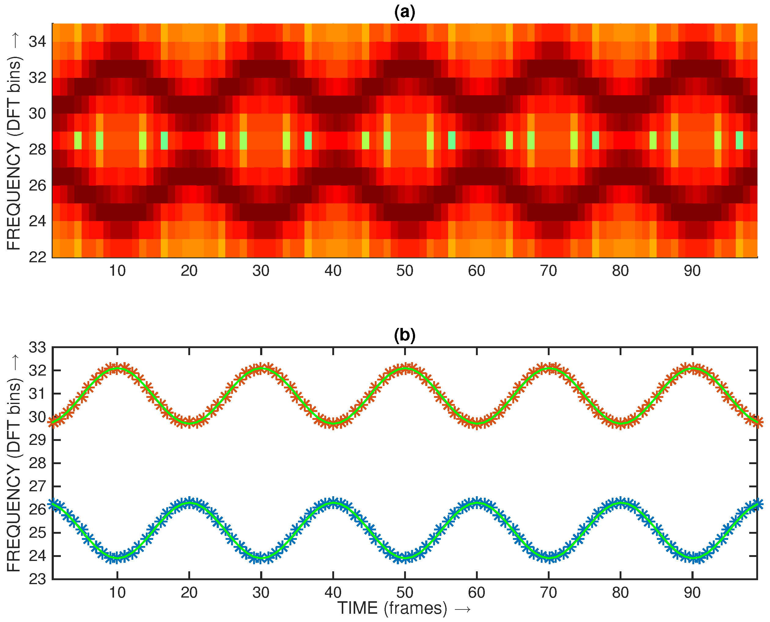
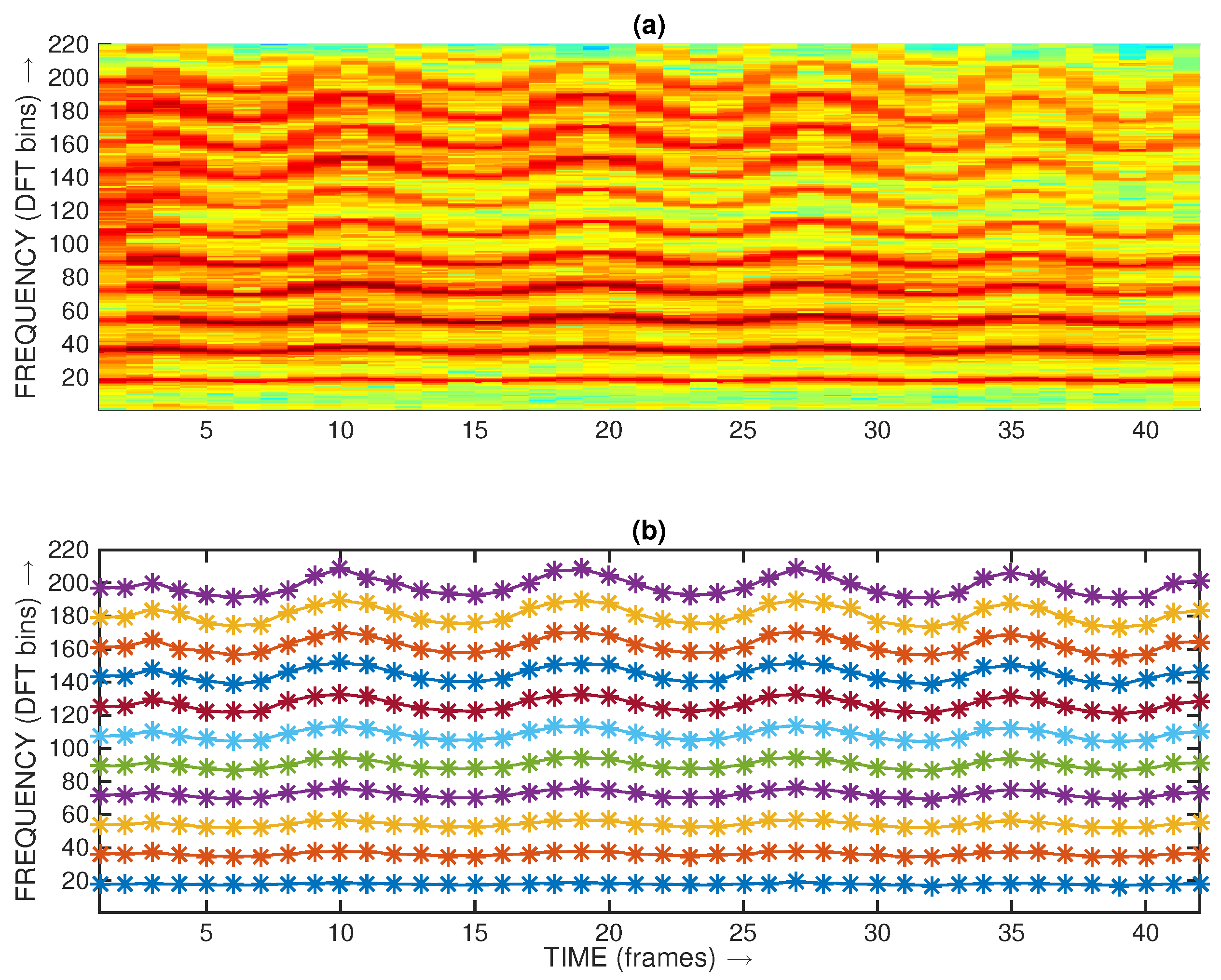
In this paper, we focus on accurate frequency estimation of individual sinusoids when they are contaminated by other interfering sinusoids, in addition to wideband noise. This is illustrated in Figure 1, which represents the spectrogram of two frequency-modulated (FM) sinusoids in close proximity. The granularity in the spectrogram representation is a consequence—and limitation—of the underlying discrete Fourier transform (DFT) frequency resolution, which hinders the detailed frequency contours of the FM sinusoids. Plot (b) in Figure 1 illustrates an accurate analysis of those contours by taking as input the same spectral information that is used in the represented spectrogram. The Matlab command file allowing us to replicate this figure is available on GitHub (https://github.com/Anibal-Ferreira/demo_AccSinFreqEst (URL accessed on 30 August 2023)).

Given that processing delay and computational complexity are important issues in real-time interactive applications, we focus on single-step (i.e., non-iterative), low-complexity, DFT-based frequency analysis and estimation that can be easily implemented on low-power platforms which have a limited processing capability.

Frequency estimation of sinusoids may be performed using either time-domain techniques or frequency-domain techniques [11]. The former are mainly based on correlation or covariance functions, and include Multiple Signal Classification (MUSIC) [12] and Estimation of Signal Parameters Via Rotational Invariance Techniques (ESPRIT) [13], which are eigenspace-based decomposition methods for the estimation of the frequencies of a known number of complex sinusoids observed in noise [14]. Despite their accuracy potential, we will not consider them in this paper due to their significant computational complexity.

On the other hand, frequency-domain estimation techniques are mainly based on the phase derivative of the DFT spectrum [15,16], on cepstral analysis [17] or on DFT spectrum peak analysis and coarse–fine frequency estimation [18,19,20]. Phase-based frequency estimators (the reader is referred to [15,21] for an overview) include phase-based vocoder techniques [22] and the reassignment estimator [23]. Both require information from at least two DFTs. It has been reported that the presence of several interfering sinusoids significantly disturbs phase-based estimators [15] (page 392) and [21].

In this paper, we focus on DFT-based coarse–fine frequency estimation, given that their computational simplicity is commensurate with that of the fast Fourier transform (FFT), i.e., $\mathcal{O}(NlogN)$ [1,15,18,20,21,24,25,26,27,28,29,30,31,32,33].

Many published approaches to frequency estimation presume a single complex exponential—or cisoid—which may be regarded as a highly simplistic scenario, given that, in this case, and contrarily to what happens in the case of a real-valued sinusoid, no mirrored spectral image of the cisoid exists on the negative frequency axis, which means that there are no leakage implications (in this paper, we designate the leakage due to the spectral mirror of a cisoid as self-leakage). Thus, a given frequency estimator may be portrayed as very accurate when operating with a cisoid under noise contamination, but its performance may drop significantly when operating with real-valued sinusoids, or even degrade critically under the influence of other co-existing sinusoids; namely, quasi-harmonic sinusoids. In fact, as pointed out by Hainsworth and Macleod [21] (page 2), ‘sinusoidal estimation errors consist of bias intrinsic to the estimation algorithm, variance from the noise, and bias due to multiple tones’. These are the real-world conditions that this paper addresses, as many signals in nature have a quasi-harmonic structure, notably singing and musical signals in general, and especially those containing musical chords (for example, piano sounds are known to exhibit a relevant degree of inharmonicity [34]).

In [35], Aboutanios et. al. present an iterative algorithm to estimate the frequency of a cisoid. This algorithm presumes the rectangular window and uses an interpolation formula that requires two additional DFT coefficients, which, in fact, correspond to Odd-DFT (ODFT) coefficients [36,37] (see also Section 3.3). This algorithm, known as the Aboutanios and Mulgrew (A&M) algorithm, exhibits a performance that is very close to the Cramér–Rao lower bound (CRLB). It has been extended in [38] to the estimation of the frequency of a real sinusoid and, in [39], to the estimation of the frequencies of multiple superimposed cisoids. In both cases, the A&M baseline algorithm is used after the leakage due to all cisoids on both positive and negative frequency axes are modeled, synthesized, and subtracted from the signal. The purpose of this processing is to leave the cisoid whose frequency is being estimated free from leakage interference.

Other published works have also addressed compensation or mitigation techniques for the bias created by harmonics above the fundamental frequency of a harmonic structure of sinusoids, which implies a significant computational penalty. For example, Liguori et al. [40] discuss compensation strategies for a single frequency estimator when the number of interfering harmonics is 2 or 4. Belega and Petri [41] discuss compensation strategies for a specific class of windows (maximum side lobe decay—MSD—windows); especially the Hanning window.

More recent work [42,43] took inspiration from the A&M algorithm and combines iterative leakage compensation techniques in order to deliver accurate frequency estimation results. For example, Liu et al. [43] combine several techniques in order to perform accurate frequency estimation of a real-valued sinusoid. Estimation is performed in two steps. In the first step, the MSD window is used in the DFT analysis for coarse frequency estimation. This estimation requires the computation of three additional DFT coefficients inside the main lobe of the frequency response of the MSD window. This process is repeated twice for improved estimation results. An interpolation formula adapted to the MSD window is then used to deliver the ‘coarse’ frequency estimation. Using this estimation, a cisoid having a negative frequency is synthesized and added to the signal, such that the resulting signal reduces to a cisoid having a positive frequency only (i.e., self-leakage is almost entirely cancelled out). Then, in a second step, this new complex-valued signal undergoes a similar processing, but using the rectangular window; DFT analysis is followed by the computation of three additional DFT coefficients inside the main lobe of the frequency response of the rectangular window, and this is a process which is again repeated twice. The final accurate frequency estimation is obtained by means of an interpolation formula that is adapted to the rectangular window.

Given that, in this paper, we focus on low-complexity frequency estimation algorithms, we regard the above approaches as not practical, in case the signal contains tens or hundreds of real-valued sinusoids, because that would require not only removing all of the mirrored spectral images on the negative frequency axis, but also all of the cisoids on the positive frequency axis, except those under analysis. Moreover, bias compensation can be framed as a deterministic process in case the harmonic relationship is strict and precise. When the relationship between the target sinusoid and the interfering sinusoids is quasi-harmonic, and the latter are further subject to amplitude modulation (AM) and frequency modulation (FM) effects, as we admit in this paper, then the interference process is more probabilistic rather than deterministic. Thus, in this paper, we do not aim to optimize further the frequency estimation performance of individual frequency estimators beyond the current state of the art, but focus instead on the intrinsic robustness and performance of a representative selection of simple and efficient frequency estimators (i.e., one-step DFT-based frequency estimators), as reported in the literature, when the target real-valued sinusoid is subject to non-deterministic and AM and FM-modulated quasi-harmonic interference, in addition to noise, both above and below the target sinusoid. To the best of our knowledge, this perspective has not yet been discussed in the literature.

In [44], the direct impact of quasi-harmonic interference on the performance of several non-iterative DFT-based frequency estimators was studied. This study was, however, limited in that only two interfering sinusoids were quasi-harmonically related to the target sinusoid, AM/FM modulation effects were not considered, and a representative comparison between frequency estimators using different windows was not made. In this paper, we expand our previous research on accurate frequency estimation of real sinusoids [6,37,44,45], and we evaluate the relative performance of a selection of nine representative (and non-iterative) DFT-based frequency estimators under mild and strong full-bandwidth quasi-harmonic interference, both below and above the target sinusoid frequency. This selection of estimators is based on their reported efficiency and performance, and also includes a modified version of a recent sine window-based frequency estimator [37,46]. Moreover, we consider that the harmonic interference is subject to AM/FM modulation effects reflecting typical perturbations in real-world signals, such as singing [47] and musical chords.

The remainder of the paper is structured as follows. In Section 2, we detail the specificities of our DFT-based frequency estimation problem, namely in terms of the signal assumptions, the analysis framework and its constraints, test settings, and the degrees of harmonic interference. We also address in this section the different window functions in our research and their features, and the performance criterion we use to assess results. In Section 3, we describe briefly all nine DFT-based frequency estimators in our research, including a recently improved version of a frequency estimator that is based on the sine window. In Section 4, we present and discuss the main results in this paper when the frequency estimation is not affected by quasi-harmonic interference, when it is full-bandwidth but mild, and when it is full-bandwidth and strong. Finally, Section 5 summarizes the main results and contributions of this paper and projects future research.

2. DFT-Based Frequency Estimation

2.1. The Estimation Problem

We consider that $x\left[n\right]$ represents a discrete-time signal containing a target sinusoid whose frequency is ${\omega }_{\mathsf{\ell }}$, and that is affected by additive white Gaussian noise, $r\left[n\right]$, and, possibly also, other co-existing sinusoidal components that are quasi-harmonically related. These are generally represented by $s\left[n\right]$.

The frequency of the target sinusoid is given by

$${\omega }_{\mathsf{\ell }}=\frac{2\pi }{N}(\mathsf{\ell }+{\mathrm{\Delta }}_{\mathsf{\ell }}),$$

(1)

where ℓ and ${\mathrm{\Delta }}_{\mathsf{\ell }}$ represent, respectively, the integer part (or the DFT bin index, $0<\mathsf{\ell }<N/2$), and the fractional part on the DFT bin scale ($0.0\le {\mathrm{\Delta }}_{\mathsf{\ell }}<1.0$ or, depending on the interpolation rule, $-0.5\le {\mathrm{\Delta }}_{\mathsf{\ell }}<0.5$), and N is the size of the DFT. In the case of a complex sinusoid (or cisoid),

$$x\left[n\right]=A{e}^{n{\omega }_{\mathsf{\ell }}+\varphi }+r\left[n\right]+s\left[n\right]$$

(2)

and, in the case of a real sinusoid,

$$x\left[n\right]=Asin\left(n{\omega }_{\mathsf{\ell }}+\varphi \right)+r\left[n\right]+s\left[n\right].$$

(3)

In both equations, A represents the magnitude of the sinusoid, and $\varphi$ represents the starting phase of the sinusoid. The estimation problem involves taking an N-sample segment of the input signal according to (2), or (3), and finding the values of ℓ and ${\mathrm{\Delta }}_{\mathsf{\ell }}$ after the signal has been multiplied by an analysis window, $h\left[n\right]$, and transformed to the frequency domain using an N-point DFT

$$V\left[k\right]=\sum _{n=0}^{N-1}h\left[n\right]x\left[n\right]e^{-j\frac{2\pi }{N}kn}.$$

(4)

Since this analysis is discrete in both time and frequency domains, $V\left[k\right]$, $x\left[n\right]$, and $h\left[n\right]$ are all N-periodic. The natural frequency resolution of the N-point DFT (or bin width) is $2\pi /N$.

It is known that when the rectangular window is used, and the size of the DFT (N) and the Signal-to-Noise Ratio (SNR) are sufficiently high, then the maximum likelihood estimate of the frequency of a sinusoid corresponds to the frequency value that maximizes the magnitude spectrum. The error variance of this estimate approaches the Cramér–Rao lower bound (CRLB) that characterizes the minimum error variance of a general unbiased estimator [25,48]. Thus, when several sinusoids co-exist, and provided that N is sufficiently high, i.e., provided that the different sinusoids are resolved by the DFT such that the magnitude spectrum consists of a multimodal function, frequency estimation can be reliably performed while avoiding computationally intensive iterative [28] or analysis-by-synthesis [2] procedures. In this context, a crude frequency estimator would just identify the local maximum in the magnitude spectrum that exists at $k=\mathsf{\ell }$, i.e., $\mathsf{\ell }=\underset{k}{\mathrm{argmax}}\left|V\left[k\right]\right|$, and estimate the frequency as ${\widehat{\omega }}_{\mathsf{\ell }}=\mathsf{\ell }2\pi /N$. This is usually referred to in the literature as coarse frequency estimation. In this worst case scenario, due to the range of ${\mathrm{\Delta }}_{\mathsf{\ell }}$, the maximum absolute estimation error is $50\%$ of the normalized bin width, i.e., $|{\widehat{\omega }}_{\mathsf{\ell }}-{\omega }_{\mathsf{\ell }}|/(2\pi /N)\le 0.5$. Given that this worst-case estimation error is a good anchor for a ‘non-accurate’ frequency interpolator, (in this paper, ‘frequency estimation’ and ‘frequency interpolation’ are used interchangeably), all results in this paper are normalized by the natural frequency resolution of the DFT ($2\pi /N$) in order to give a sense, in relative terms, on how accurate a given estimator is.

The main purpose of the estimation problem is, therefore, to find a simple and accurate algorithm, or formula, that estimates the value of ${\mathrm{\Delta }}_{\mathsf{\ell }}$ through interpolation of the values of $V\left[k\right]$ around $k=\mathsf{\ell }$, when the sinusoid is affected not only by Gaussian noise according to a given SNR, but also by different degrees of quasi-harmonic interference (no interference, mild, or strong interference). This two-step approach has been identified by Rife and Boorstyn as a “coarse search” and a “fine search” [25]. While the first step is quite straightforward (it involves only peak-picking), provided that the signal is not overwhelmed by noise, the second is not and represents, in fact, the challenge that is discussed in most DFT-based frequency estimation papers (Section 1), and also in this paper. In particular, when the sinusoid is contaminated by other sinusoids and/or noise, the maximum absolute estimation error should be far less than $50\%$ of the normalized bin width, and the variance of the estimation error should approach as much as possible the CRLB [30,49]. As explained in Section 2.3, in addition to evaluating the relative performance between different estimators under the same test conditions, we are especially interested in assessing how the relative performance changes when there is no harmonic interference, when the quasi-harmonic interference is mild, or when it is strong. This represents a stress test that unveils how consistent the accuracy and robustness of a given frequency estimator remains under real-world conditions.

In this context, and as we will address in Section 2.5, in our research we focus on the challenge that is represented by (3) because it reflects more realistic real-world conditions.

2.2. Estimation Constraints

One good example of our target applications is real-time visual feedback of the singing voice and, notably, of the associated melodic line [3,50]. This scenario implies that the total processing delay, from the instant the signal is captured using a microphone, till the instant its information is represented on a computer screen, is commensurate with the human perception of ‘instantaneous’. Therefore, the acceptable total processing delay should not exceed a few tens of milliseconds. This is quite in line with the acceptable delay between sound and image before the ‘lip sync’ problem is perceived by a human, or the maximum acceptable delay between the direct sound and a reflected replica before the latter is perceived as a distinct echo [51]. In both cases, acceptable delays may range between 10 ms and about 50 ms. On the other hand, the syllabic duration in speech is at least 10–20 ms [52], and while in singing it tends to be longer, ornamental elements in singing like vibrato mean that important pitch variations should be accurately captured and represented on a screen with a reasonable refresh rate, or time resolution; for example, in the order of 20 ms.

Both aspects, real-time operation and time resolution in signal analysis, and refresh rate, require that the total processing delay should not exceed 50 ms, and that all processing stages should be as parsimonious as possible regarding computational complexity. Therefore, taking advantage of the local stationarity of speech, or singing, a convenient solution to the frequency estimation problem involves using a single DFT and an accurate and computationally efficient frequency estimation procedure. We admit that all individual sinusoidal components that may exist in the signal are eligible for accurate frequency estimation. For example, this is important in order to facilitate segregation of multiple co-existing harmonic structures (as in musical chords). In this perspective, frequency estimation must be carried using an algorithm that:

• Excludes iterative procedures and is computationally light;
• Computes a DFT whose length is the same as that of the data vector, i.e., zero-padding techniques ([20,33,53,54]) are excluded (zero-padding can be looked at as an inefficient frequency interpolation technique);
• Maximizes the estimation accuracy and robustness when other interfering sinusoids co-exist in the signal, in addition to noise.

According to these general guidelines, our approach to sinusoidal analysis and frequency estimation involves three fundamental steps:

• Multiplication of a signal (or data) vector $x\left[n\right]$ by a window function that is represented by $h\left[n\right]$ (an operation also known as tapering);
• DFT computation, typically by means of an FFT;
• Peak picking in the DFT magnitude spectrum and frequency estimation of a target sinusoid by using a simple interpolation algorithm (or formula), taking several samples from the DFT magnitude spectrum.

2.3. Degrees of Harmonic Interference and Test Settings

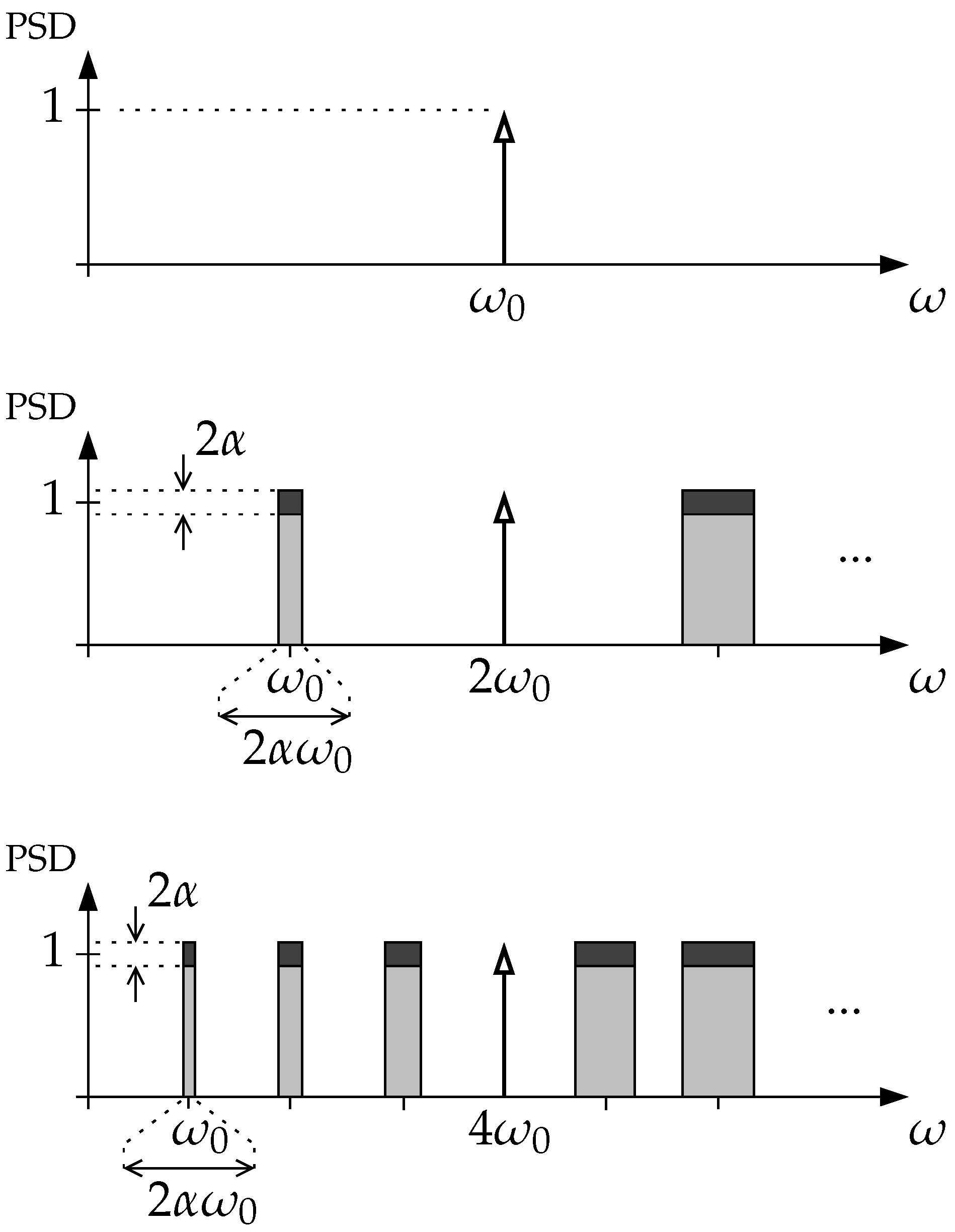
In our research, we will consider three levels of severity for the quasi-harmonic interference that is represented in (3) by $s\left[n\right]$: no interference, mild interference, or strong interference. While the first case is obvious (i.e., there are no other sinusoids than that whose frequency is being estimated), the second and third severity levels can be explained with the help of Figure 2. Given a target sinusoid frequency to be estimated, according to (1), we consider that, under mild harmonic interference, the target frequency is approximately the second harmonic of an existing quasi-harmonic structure, and, under strong harmonic interference, the same target frequency is approximately the fourth harmonic of an existing quasi-harmonic structure of sinusoids. The fundamental frequency of the quasi-harmonic structure is ${\omega }_0=\frac{2\pi }{N}{F}_0$, where $F_0$ represents a real number on a DFT bin scale, with $0<F_0<N/2$. In our simulations, we set $\mathsf{\ell }=20$ and, using a simple frequency spacing condition simulating quasi-harmonicity, $3F_0-(\mathsf{\ell }+1.0)=\mathsf{\ell }-F_0$, we obtain that for mild harmonic interference, $F_0=10.25$ DFT bins. For strong harmonic interference, we consider that $F_0$ is half of this value, i.e., $F_0=5.125$ DFT bins. As explained in Section 2.4, these two $F_0$ alternatives ensure that, for the different windows that we consider in our research, harmonic resolvability is guaranteed, although tightly in some cases.

In order to give the quasi-harmonic interference a realistic profile, we consider that it is also affected by AM and FM effects according to a modulation index, $\alpha$, as it is represented in Figure 2. As a reference, we use characteristics that are typical in singing. In fact, singing signals are frequently characterized by a periodic variation of the fundamental frequency, an FM effect known as vibrato, as well as a periodic variation of the signal intensity, an AM effect known as tremolo. Perceptually, tremolo is not as important as vibrato [47] and, to a certain extent, the former can be looked at as a consequence of the latter. In fact, tremolo depends on several factors; namely, the relation between the frequencies of partials (i.e., the harmonics), and the frequencies of voice formants [47]. Therefore, it is a reasonable assumption that the rate of vibrato and tremolo is the same. Sundberg [47] (page 164) notes that a typical and comfortable vibrato rate is 6.5 Hz, and that the typical extension of the vibrato is 1.5 semitones on the equally tempered scale. This corresponds to a relative variation of the fundamental frequency by about ${\left(\sqrt[12]{2}\right)}^{1.5}-1.0\approx 9.1\%$. Therefore, we consider in our tests that the quasi-harmonic interference occupies the full Nyquist bandwidth and is subject to a combined AM and FM effect whose depth is $4.5\%$ around the mean, and whose rate is 6.5 Hz, respectively.

In this context, the quasi-harmonic interference $s\left[n\right]$ in (3) is obtained as

$$s\left[n\right]=A\left(1+a\left[n\right]\right)\sum _{\begin{array}{c}k=1\\ k\ne \mathrm{nint}\left\{\frac{\mathsf{\ell }}{F_0}\right\}\end{array}}^{\lfloor \frac{N/2}{F_0}\rfloor }sin\left[k{F}_0\left(\frac{2\pi }{N}n+f\left[n\right]\right)\right],$$

(5)

where $\lfloor ·\rfloor$ denotes the “floor” operator retaining the largest integer in the argument, $\mathrm{nint}\{·\}$ denotes the nearest integer, the frequency of the target sinusoid is ${\omega }_{\mathsf{\ell }}=\frac{2\pi }{N}(\mathsf{\ell }+{\mathrm{\Delta }}_{\mathsf{\ell }})$ with $\mathsf{\ell }=20.0$, and ${\mathrm{\Delta }}_{\mathsf{\ell }}$ varies in the range $[0.0,1.0[$. We set $A=1$, which means that all partials in the harmonic interference have a magnitude that is comparable to that of the target sinusoid. This denotes a condition that typically is more demanding than what happens with real-world signals. In (5) the quasi-harmonic interference is AM and FM modulated using

$$a\left[n\right]=\alpha sin\left(\frac{2\pi }{N}\theta n+{\varphi }_{\mathrm{AM}}\right),$$

(6)

and

$$f\left[n\right]=\beta sin\left(\frac{2\pi }{N}\theta n+{\varphi }_{\mathrm{FM}}\right).$$

(7)

In these equations, we set $N=512$, and we assume that the sampling frequency is 22,050 Hz. Moreover, taking into consideration the discussion above regarding the rate of vibrato, we set $\theta =\frac{6.5\times 512}{\mathrm{22,050}}\approx 0.151$. Regarding the depth of the AM/FM modulation effects, we set $\alpha =0.045$, which determines $\beta =\frac{\alpha }{\theta }\approx 0.298$.

For each value of ${\mathrm{\Delta }}_{\mathsf{\ell }}$ in the range $[0.0,1.0[$ and using a step of $0.01$, 100 Monte Carlo realizations of the (real) noise vector $r\left[n\right]$ are generated according to a desired SNR (in the range $[-10,70]$ dB, in steps of $2.5$ dB), in order to collect stable statistics. In each realization of $r\left[n\right]$ and, therefore, of $x\left[n\right]$, the values of $\varphi$, ${\varphi }_{\mathrm{AM}}$, and ${\varphi }_{\mathrm{FM}}$ are randomized in the range $[0,2\pi [$, which represents an important part of the Monte Carlo simulations.

2.4. Windows, Selectivity and Leakage

In general, our target applications involve accurate frequency estimation in multitone detection and estimation. In this case, as noted by Harris [55], ‘maximum dynamic range in multitone detection requires the Fourier transform of the window to exhibit a highly concentrated central lobe with very low sidelobe structure’. We illustrate this using four windows of decreasing selectivity and increasing main-side lobe attenuation: the rectangular window

$$h_R\left[n\right]=1,n=0,1,\dots ,N-1,$$

(8)

the sine window

$$h_S\left[n\right]=\sqrt{h_H\left[n\right]}=sin\frac{\pi }{N}(n+0.5),n=0,\dots ,N-1,$$

(9)

the shifted Hanning window that is defined as

$$h_H\left[n\right]=\frac{1}{2}\left[1-cos\frac{2\pi }{N}(n+0.5)\right],n=0,\dots ,N-1,$$

(10)

and the Gaussian window

$$h_G\left[n\right]=exp\left[-\frac{1}{2}{\left(\gamma \frac{n-M}{M}\right)}^2\right],n=0,\dots ,N-1,$$

(11)

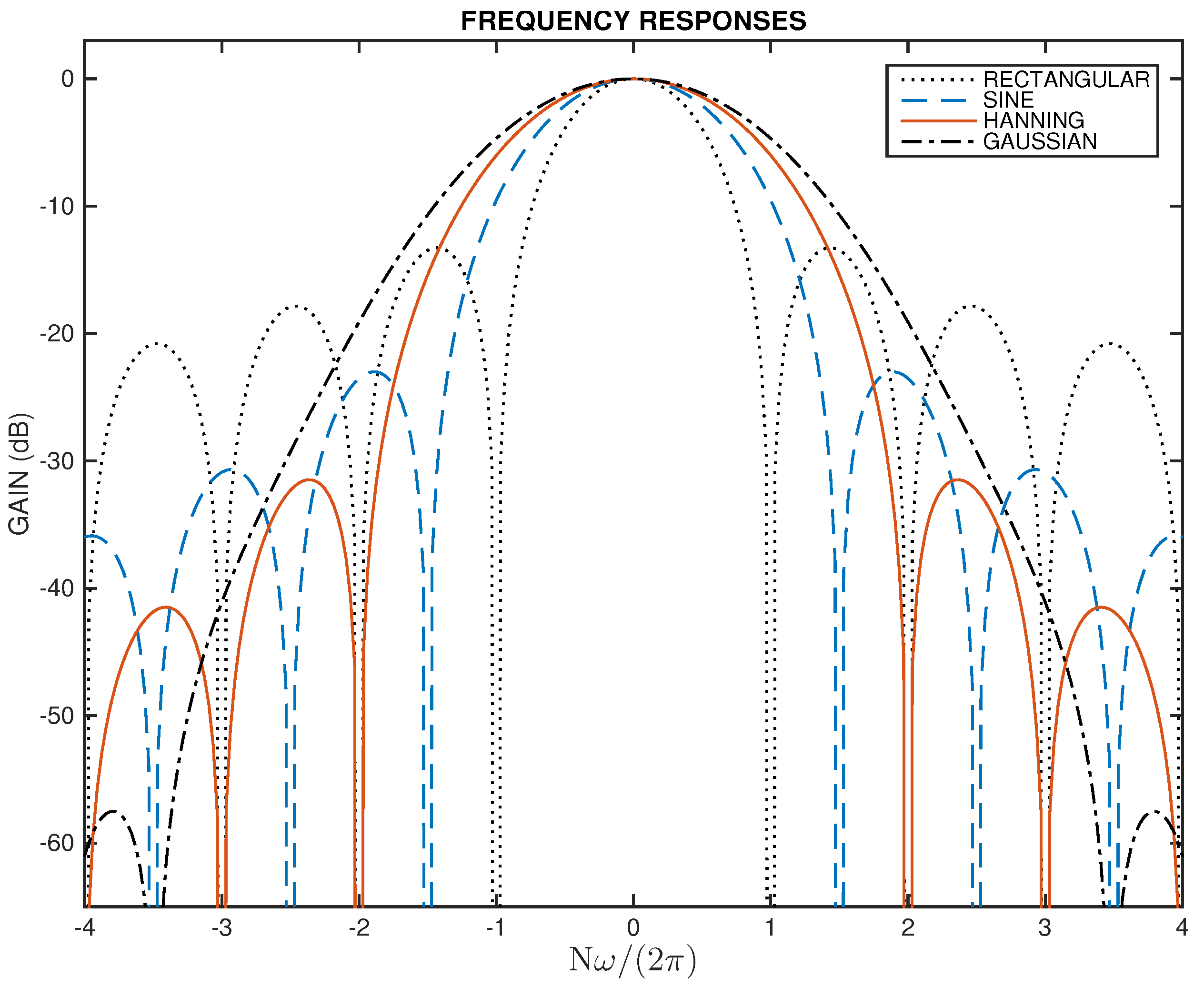
where $M=(N-1)/2$. Figure 3 illustrates the magnitude of the frequency responses of these windows. Due to its importance regarding the optimized tradeoff between time and frequency localization in connection with the uncertainty principle [55], the Gaussian window we are illustrating here presumes $\gamma =3.0$.

Figure 3 shows that the main lobe width of the frequency response of the rectangular, sine, Hanning, and Gaussian window is $4\pi /N$, $6\pi /N$, $8\pi /N$, and $14\pi /N$, respectively. This can also be seen as the safe frequency separation between two sinusoids so that they are fairly resolved in the DFT discrete frequency domain, i.e., that allows the two sinusoids to appear as individual peaks in the DFT magnitude spectrum.

In this perspective, the rectangular window has the best selectivity and the Gaussian window has the poorest selectivity. On the other hand, the larger the main lobe, the better the attenuation between the main lobe and the side lobes; a feature referred to as ‘near-end leakage’ [56]. It is known that the minimum main-side lobe attenuation of the rectangular, sine, Hanning, and Gaussian windows, is about 13 dB, 23 dB, 32 dB, and 57 dB, respectively [55]. In this perspective, the rectangular window gives rise to the largest leakage and the Gaussian window gives rise to the smallest leakage. The lower the leakage, the smaller the mutual influence between two resolved sinusoids in the discrete Fourier transform (DFT) spectrum [56]. In fact, Hainsworth and Macleod note that ‘windowing increases variance but reduces bias’ [21]. These aspects are very important in this paper as they are likely to influence the performance of the estimation process when other interfering sinusoids and noise are present in the signal. The sine window is particularly important in audio analysis/synthesis and coding [9,57,58], since it is frequently used in analysis/synthesis filter banks satisfying perfect reconstruction requirements [59,60] (e.g., the Modified Discrete Cosine Transform—MDCT [59,60,61]). A different type of sine window is considered in [62] in the estimation of the frequency of a damped co-sinusoid.

Figure 3 also helps us to understand that a single stationary cisoid gives rise to a local peak in the DFT magnitude spectrum that, at most, comprises two, three, four, or seven DFT bins falling within the main lobe of the frequency response of the rectangular, sine, Hanning, or Gaussian window, respectively. Thus, in order to avoid leakage as much as possible, it appears appropriate to interpolate the value of ${\mathrm{\Delta }}_{\mathsf{\ell }}$ using at most the two, three, four, or seven largest DFT spectral lines around a spectral peak when the rectangular, sine, Hanning, or Gaussian window is used, respectively (other methods require at least 6 or even 18 DFT bins [18]). In our simulations, we are not considering the Gaussian window, since all results with the quadratic interpolation rule in the frequency domain (quadratic—or parabolic—interpolation is strictly accurate only for the Gaussian window [53] (page 47)) consistently revealed that it has a relative poor performance. Thus, only the rectangular, sine, and (shifted) Hanning windows are considered in our simulations and results.

2.5. Performance Criterion

The CRLB for the variance of the frequency estimation error when a complex sinusoid (or cisoid) is considered, and an unbiased estimator is used, is given by [25,30,49]

$$\mathrm{var}\left\{{\omega }_{\mathsf{\ell }}-{\widehat{\omega }}_{\mathsf{\ell }}\right\}\ge \frac{6{\sigma }^2}{A^{2}N(N^2-1)},$$

(12)

where A represents the magnitude of the cisoid, N represents the period of the DFT, and ${\sigma }^2$ represents the variance of the noise which is assumed to be zero-mean, white, complex, and Gaussian. However, using a cisoid as a test signal corresponds to the best test scenario since simple frequency estimators can be found that either provide exact estimates in the absence of noise or other interferences, or that perform quite close to the CRLB when noise affects the signal, as discussed in Section 1, and as noted at the end of Section 2.1. This scenario is assumed, for example, in [20,27,30,31].

If $x\left[n\right]$ is instead a real sinusoid according to (3), the magnitude spectrum of $V\left[k\right]$ exhibits two local maxima (i.e., spectral peaks) that are governed by Dirichlet kernels [55,63], for example of the form $sin\left(\theta \right)/sin(\theta /N)$ in the case of the rectangular window, with one of them being on the positive frequency axis, and the other one being in the ‘mirror’ position on the negative frequency axis. Figure 3 illustrates the magnitude of the Dirichlet kernel (on a dB scale) for different windows. Each spectral peak generates leakage that influences the ‘mirror’ peak and that may be significant if ℓ is a ‘small’ number, for example, less than 5 DFT bins in the case of the rectangular window [26,27], or less than 9 DFT bins in the case of the Hanning window [18].

Most frequency estimators presume that leakage due to the image of a spectral peak (i.e., the self-leakage) can be ignored, which means that they suffer from a structural bias that sets a limit to the performance of the estimator [15] (page 391). Despite this, and as noted by Betser et. al. [22] (page 513), the CRLB for a single cisoid and unbiased estimators is still a useful reference for biased estimators. One possibility to convert the input real sinusoids and noise to their complex versions is to construct an analytical signal using the Hilbert transform [15,25]. However, because a practical Hilbert transform modifies the signal near the zero and Nyquist frequencies, in addition to increasing the overall algorithm complexity, it is not considered here.

Furthermore, many real-world signals of great interest, such as speech, or singing, exhibit an approximate harmonic structure and, therefore, each spectral peak, in addition to being influenced by its mirror spectral image, is also influenced by leakage due to neighboring (and interfering) sinusoids. Assessing the robustness of different frequency estimators to different levels of this combined influence, in addition to noise, is, thus, the purpose of this paper.

In this scenario, we create a performance criterion that is based on the CRLB and that assumes that all sinusoids and noise, are real-valued. Given that there is only one target real-valued sinusoid whose frequency is estimated, according to the model of (3), the CRLB becomes scaled by a factor of 2. In addition, and in order to simplify the evaluation of the relative performance of different frequency interpolators, as discussed in Section 2.1, we take the square root of $\mathrm{var}\left\{{\omega }_{\mathsf{\ell }}-{\widehat{\omega }}_{\mathsf{\ell }}\right\}$, and we normalize the result by the natural frequency resolution of the DFT ($2\pi /N$):

$$\mathrm{RMSE}=\sqrt{2}\frac{\sqrt{\mathrm{var}\left\{{\omega }_{\mathsf{\ell }}-{\widehat{\omega }}_{\mathsf{\ell }}\right\}}}{2\pi /N}\ge \sqrt{\frac{3{\sigma }^2}{A^2{\pi }^{2}N(1-1/N^2)}}.$$

(13)

Thus, this performance criterion is not only based on the well established CRLB, but it also offers a clear meaning: if, for some frequency estimator, the corresponding RMSE is closer to $0.5$ (i.e., 50% of the DFT bin width), that means that its performance is poor and non-accurate. On the other hand, if the corresponding RMSE is closer to the normalized CRLB bound, that means that its performance is closer to the ideal performance. The RMSE criterion will be used in Section 4 when the main results of this paper will be presented and discussed.

3. Tested Frequency Estimators

In this section, we describe the frequency estimators that are included in our research. We organize this description by groups of frequency estimators as a function of the windows they use. Their relative performance combining accuracy and sensitivity to noise and harmonic interference will be evaluated in Section 4 using the RMSE criterion. All frequency estimators use information from a few bins surrounding a spectral peak in the DFT magnitude spectrum, the DFT length is the same as that of the data vector, and all of them comply with the preferred structural characteristics that are identified in Section 2.2. As indicated in Section 2.1, since the integer part of the frequency is easily found by locating a local maximum in the magnitude spectrum, all frequency estimators are mainly concerned with estimating the fractional frequency ${\widehat{\mathrm{\Delta }}}_{\mathsf{\ell }}$ using the $V\left[k\right]$ spectral information.

3.1. Rectangular Window-Based Estimators

Two non-iterative, DFT-based frequency estimators that presume the rectangular window have been selected in our research based on their reported simplicity and performance [1,30,64]. These frequency estimators are identified as Macleod98(R) and Jacobsen07(R). Both estimators use three samples from the DFT spectrum [30,44], including magnitude and phase information. This means that, in addition to the two samples that fall within the main lobe of the frequency response of the rectangular window, one more sample that belongs to one of side lobes is also used. This specific perspective has not been discussed by the authors.

If $\left|V\right[\mathsf{\ell }\left]\right|$ corresponds to a local maximum in the DFT magnitude spectrum, and if $\Re \{·\}$ denotes the real part of the complex argument, then the Macleod98(R) frequency estimator first computes $\alpha =\Re \left\{V\left[\mathsf{\ell }\right]V^{*}\left[\mathsf{\ell }\right]\right\}$, ${\alpha }_L=\Re \left\{V[\mathsf{\ell }-1]V^{*}\left[\mathsf{\ell }\right]\right\}$, and ${\alpha }_R=\Re \left\{V[\mathsf{\ell }+1]V^{*}\left[\mathsf{\ell }\right]\right\}$, which allows us to obtain

$$\gamma =\frac{{\alpha }_L-{\alpha }_R}{2\alpha +{\alpha }_L+{\alpha }_R},$$

and then, finally

$${\widehat{\mathrm{\Delta }}}_{\mathsf{\ell }}=\frac{\sqrt{1+8{\gamma }^2}-1}{4\gamma },-\frac{1}{2}\le {\widehat{\mathrm{\Delta }}}_{\mathsf{\ell }}<\frac{1}{2}.$$

(14)

In the case of the Jacobsen07(R) frequency estimator, frequency estimation is simply obtained by computing

$$\begin{array}{c}\hfill {\widehat{\mathrm{\Delta }}}_{\mathsf{\ell }}=\frac{tan\frac{\pi }{N}}{\frac{\pi }{N}}\Re \left\{\frac{V[\mathsf{\ell }-1]-V[\mathsf{\ell }+1]}{2V\left[\mathsf{\ell }\right]-V[\mathsf{\ell }+1]-V[\mathsf{\ell }-1]}\right\},\\ \hfill -\frac{1}{2}\le {\widehat{\mathrm{\Delta }}}_{\mathsf{\ell }}<\frac{1}{2}.\end{array}$$

(15)

In this equation, a correction factor, which was proposed by Candan in order to reduce bias and improve performance [64], has been included.

3.2. Hanning Window-Based Estimators

Based on their reported simplicity and performance, we selected four non-iterative DFT-based frequency estimators that presume the Hanning window [1,27,30,32]. They are identified in this paper as Grandke83(H), Macleod98(H), Quinn06(H), and Jacobsen07(H).

The Grandke83(H) frequency estimator uses spectral magnitude information only and is implemented by computing

$${\widehat{\mathrm{\Delta }}}_{\mathsf{\ell }}=\frac{2\left|V\right[\mathsf{\ell }+1\left]\right|-\left|V\right[\mathsf{\ell }\left]\right|}{\left|V\right[\mathsf{\ell }+1\left]\right|+\left|V\right[\mathsf{\ell }\left]\right|},0\le {\widehat{\mathrm{\Delta }}}_{\mathsf{\ell }}<1.$$

(16)

The author admits that good performance requires that real sinusoids are sufficiently separated in frequency, e.g., by more than 20 DFT bins. Therefore, it is important to assess how the performance compares to that of other estimators when this constraint is relaxed under quasi-harmonic interference.

The Macleod98(H) frequency estimator uses the same $\alpha$, ${\alpha }_L$, and ${\alpha }_R$ coefficients that were defined in the previous section and delivers the fractional frequency as

$${\widehat{\mathrm{\Delta }}}_{\mathsf{\ell }}=2\frac{{\alpha }_L-{\alpha }_R}{2\alpha -{\alpha }_L-{\alpha }_R},-\frac{1}{2}\le {\widehat{\mathrm{\Delta }}}_{\mathsf{\ell }}<\frac{1}{2}.$$

(17)

The author emphasizes that this estimator benefits from the ‘intrinsic leakage rejection’ of the Hanning window [30].

The Quinn06(H) frequency estimator uses the three DFT samples surrounding the local maximum in the magnitude spectrum ($\left|V\right[\mathsf{\ell }\left]\right|$) [32]. Defining ${\alpha }_L=\frac{2\rho +1}{1-\rho }$ where $\rho =\Re \left\{\frac{V[\mathsf{\ell }-1]}{V\left[\mathsf{\ell }\right]}\right\}$, and ${\alpha }_R=\frac{2\varrho +1}{\varrho -1}$ where $\varrho =\Re \left\{\frac{V[\mathsf{\ell }+1]}{V\left[\mathsf{\ell }\right]}\right\}$, frequency is estimated as

$${\widehat{\mathrm{\Delta }}}_{\mathsf{\ell }}=\frac{{\alpha }_L+{\alpha }_R}{2}+\xi \left({\alpha }_L^2\right)-\xi \left({\alpha }_R^2\right),-\frac{1}{2}\le {\widehat{\mathrm{\Delta }}}_{\mathsf{\ell }}<\frac{1}{2},$$

(18)

where

$$\begin{array}{ccc}\hfill \xi \left(x\right)& =& -\frac{5}{14}log(35x^2+120x+32)+\hfill \\ & & \frac{\sqrt{155}}{140}log\left(\frac{12+7x-4\sqrt{\frac{31}{5}}}{12+7x+4\sqrt{\frac{31}{5}}}\right).\hfill \end{array}$$

The Jacobsen07(H) frequency estimator uses spectral magnitude information only and is implemented by computing

$$\begin{array}{c}\hfill {\widehat{\mathrm{\Delta }}}_{\mathsf{\ell }}=1.36\frac{\left|V\right[\mathsf{\ell }+1\left]\right|-\left|V\right[\mathsf{\ell }-1\left]\right|}{\left|V\right[\mathsf{\ell }\left]\right|+\left|V\right[\mathsf{\ell }+1\left]\right|+\left|V\right[\mathsf{\ell }-1\left]\right|},\\ \hfill -\frac{1}{2}\le {\widehat{\mathrm{\Delta }}}_{\mathsf{\ell }}<\frac{1}{2}.\end{array}$$

(19)

It consists of one of the two Hanning window-based fractional frequency estimators that are proposed in [1].

3.3. Sine Window-Based Estimators

We include in our simulations three sine window-based frequency estimators. The first version of these frequency estimators was presented in [6] and was based on a single ArcTan-based approximation rule (this is not related to the ArcTan-based estimator that is presented in [15]), which provided a maximum absolute estimation error of 1%, relative to the natural frequency resolution of the DFT filter bank (i.e., of the DFT bin width) and in the absence of noise. A subsequent improvement of this frequency estimator was based on three ArcTan-based approximation rules, which brought the maximum absolute estimation error down to 0.1% of the bin width [37]. This estimator is identified in our tests as ArcTan(S). Subsequently, Dun and Liu [46] found more practical approximations to the three rules and, using essentially the same design approach of [37], obtained a frequency estimator which exhibits a maximum absolute estimation error slightly below 0.025% of the DFT bin width. The frequency estimator modified by Dun–Liu is identified in this paper as Dun15(S).

In this paper, we also present an improvement of the estimator modified by Dun–Liu and which reduces further the maximum absolute estimation error to less than 0.006% of the DFT bin width. The context for that improvement is provided next.

Except for a constant gain factor, the magnitude frequency response of the sine window (Equation (9)) can be expressed as [37,46]

$$\left|H_S\left(\omega \right)\right|=\left|\frac{cos(N\omega /2)cos(\omega /2)}{cos\left(\omega \right)-cos(\pi /N)}\right|.$$

(20)

The sine window-based frequency estimators take advantage of the relationship between this frequency response and the magnitude spectrum as available from $\left|V\right[k\left]\right|$, since the latter is governed by the former. Figure 4 helps to illustrate that relationship according to a filter bank perspective.

This figure presumes that the frequency of the target sinusoid is ${\omega }_{\mathsf{\ell }}=\frac{2\pi }{N}(\mathsf{\ell }+{\mathrm{\Delta }}_{\mathsf{\ell }})$ (with $0.0\le {\mathrm{\Delta }}_{\mathsf{\ell }}<1.0$), and that instead of the DFT, the discrete time-frequency transformation is achieved by means of the Odd-frequency DFT (ODFT) [36]. The ODFT consists of a slight modification of (4), in the sense that the exponent in the complex exponential, $-j\frac{2\pi }{N}kn$, is replaced by $-j\frac{2\pi }{N}(k+\frac{1}{2})n$; please see [37,46,65] for details. We denote this time-frequency transformation as $V_O\left[k\right]$. The net effect of this convenient modification is that the sampled frequencies of the ODFT channels (or sub-band filters) are right-shifted by $\pi /N$ relative to those of the plain DFT, which means that when ${\mathrm{\Delta }}_{\mathsf{\ell }}\to 0.0$, or when ${\mathrm{\Delta }}_{\mathsf{\ell }}\to 1.0$, the target sinusoid is projected into two non-zero ODFT spectral lines, as Figure 4 helps to clarify (the figure represents the positive side of the frequency axis). In addition, when ${\mathrm{\Delta }}_{\mathsf{\ell }}$ varies in the range $[0.0,1.0[$, the magnitude of the ODFT channel when $k=\mathsf{\ell }$ (i.e., $V_O\left[\mathsf{\ell }\right]$) is always larger than that of the two neighboring channels (i.e., those corresponding to the ODFT channels $k=\mathsf{\ell }-1$ and $k=\mathsf{\ell }+1$). Since the magnitude of $V_O\left[k\right]$ is determined by the frequency response of the $k\mathrm{th}$ ODFT channel (except for a constant scaling factor), then the ratios involving $V_O\left[k\right]$ spectral coefficients when $k=\mathsf{\ell }-1,\mathsf{\ell },\mathsf{\ell }+1$, assuming that leakage effects are negligible, are the same as the ratios involving the frequency responses of the corresponding ODFT sub-bands or channels, as Figure 4 illustrates.

Given that the main lobe of the frequency response of $h_S\left[n\right]$ encompasses three discrete-frequency bins (Section 2.4), this creates an opportunity for three ratios involving different pairs of ODFT spectral coefficients to be computed, as specified by (21), (22), and (23). As it is illustrated in Figure 4, these ratios are the same as the frequency response ratios that are also indicated in (21), (22), and (23), and which take advantage of (20) and of the approximation $sin\left(\theta \right)\approx \theta$ for small $\theta$. Please see [37,46] for details.

$$\begin{array}{ccc}\hfill R& =& \frac{|V_O[\mathsf{\ell }-1]|}{|V_O[\mathsf{\ell }+1]|}=\frac{|H_S\left(\frac{2\pi }{N}({\mathrm{\Delta }}_{\mathsf{\ell }}+\frac{1}{2})\right)|}{|H_S\left(\frac{2\pi }{N}({\mathrm{\Delta }}_{\mathsf{\ell }}-\frac{3}{2})\right)|}\hfill \\ & \approx & \frac{(2-{\mathrm{\Delta }}_{\mathsf{\ell }})({\mathrm{\Delta }}_{\mathsf{\ell }}-1)}{{\mathrm{\Delta }}_{\mathsf{\ell }}(1+{\mathrm{\Delta }}_{\mathsf{\ell }})}\hfill \end{array}$$

(21)

$$\begin{array}{ccc}\hfill Q& =& \frac{|V_O[\mathsf{\ell }-1]|}{|V_O\left[\mathsf{\ell }\right]|}=\frac{|H_S\left(\frac{2\pi }{N}({\mathrm{\Delta }}_{\mathsf{\ell }}+\frac{1}{2})\right)|}{|H_S\left(\frac{2\pi }{N}({\mathrm{\Delta }}_{\mathsf{\ell }}-\frac{1}{2})\right)|}\hfill \\ & \approx & \frac{{\mathrm{\Delta }}_{\mathsf{\ell }}-1}{1+{\mathrm{\Delta }}_{\mathsf{\ell }}}\hfill \end{array}$$

(22)

$$\begin{array}{ccc}\hfill S& =& \frac{|V_O[\mathsf{\ell }+1]|}{|V_O\left[\mathsf{\ell }\right]|}=\frac{|H_S\left(\frac{2\pi }{N}({\mathrm{\Delta }}_{\mathsf{\ell }}-\frac{3}{2})\right)|}{|H_S\left(\frac{2\pi }{N}({\mathrm{\Delta }}_{\mathsf{\ell }}-\frac{1}{2})\right)|}\hfill \\ & \approx & \frac{{\mathrm{\Delta }}_{\mathsf{\ell }}}{2-{\mathrm{\Delta }}_{\mathsf{\ell }}}\hfill \end{array}$$

(23)

These relations can be easily solved for ${\mathrm{\Delta }}_{\mathsf{\ell }}$ leading to (24), (25), and (26), respectively.

$${\widehat{\mathrm{\Delta }}}_{\mathsf{\ell }}\approx \frac{3+R-\sqrt{1+R(14+R)}}{2(1-R)}$$

(24)

$${\widehat{\mathrm{\Delta }}}_{\mathsf{\ell }}\approx \frac{1-Q}{1+Q}$$

(25)

$${\widehat{\mathrm{\Delta }}}_{\mathsf{\ell }}\approx \frac{2S}{1+S}$$

(26)

Dun and Liu follow an approach similar to [37] and use (25) when ${\widehat{\mathrm{\Delta }}}_{\mathsf{\ell }}<0.4$, (26) when ${\widehat{\mathrm{\Delta }}}_{\mathsf{\ell }}>0.6$, and (24) when $0.4\le {\widehat{\mathrm{\Delta }}}_{\mathsf{\ell }}\le 0.6$; for details please see [46]. Many experiments led us to the conclusion that this choice of a mutually exclusive arrangement of rules not only tends to give rise to an asymmetric error distribution in the full ${\mathrm{\Delta }}_{\mathsf{\ell }}$ range, i.e., $0.0\le {\mathrm{\Delta }}_{\mathsf{\ell }}<1.0$, but also tends to aggravate bias effects due to the influence of quasi-harmonic sinusoids. We concluded that both aspects are better addressed when mutual exclusion of rules is relaxed, and at least two rules are combined in specific ranges. While avoiding overfitting for specific scenarios, we concluded that a good compromise for many different SNR and harmonic interference conditions can be obtained by combining the estimates provided by (24) and (25) when ${\widehat{\mathrm{\Delta }}}_{\mathsf{\ell }}\le 0.350$, (24) and (26) when ${\widehat{\mathrm{\Delta }}}_{\mathsf{\ell }}\ge 0.65$, and combining all three rules when $0.35<{\widehat{\mathrm{\Delta }}}_{\mathsf{\ell }}<0.65$. Equation (27) explicits these combinations that rely on a weighted average depending on the ODFT spectral coefficients, which provides a natural smoothing between the three rules.

$${\widehat{\mathrm{\Delta }}}_{\mathsf{\ell }}=\left\{\begin{array}{ccc}\hfill \frac{Q|V_O[\mathsf{\ell }-1]|+R|V_O\left[\mathsf{\ell }\right]|}{|V_O[\mathsf{\ell }-1]|+|V_O\left[\mathsf{\ell }\right]|}& ,\hfill & \hfill 0.0\le {\widehat{\mathrm{\Delta }}}_{\mathsf{\ell }}\le 0.35\\ \hfill \frac{Q|V_O[\mathsf{\ell }-1]|+R|V_O\left[\mathsf{\ell }\right]|+S|V_O[\mathsf{\ell }+1]|}{|V_O[\mathsf{\ell }-1]|+|V_O\left[\mathsf{\ell }\right]|+|V_O[\mathsf{\ell }+1]|}& ,\hfill & \hfill 0.35<{\widehat{\mathrm{\Delta }}}_{\mathsf{\ell }}<0.65\\ \hfill \frac{R|V_O\left[\mathsf{\ell }\right]|+S|V_O[\mathsf{\ell }+1]|}{|V_O\left[\mathsf{\ell }\right]|+|V_O[\mathsf{\ell }+1]|}& ,\hfill & \hfill 0.65\le {\widehat{\mathrm{\Delta }}}_{\mathsf{\ell }}<1.0\end{array}\right.$$

(27)

This equation expresses our improved sine window-based estimator, which we identify in this paper as Proposed(S). Figure 5 illustrates a practical (and reproducible) example of using (27) in order to perform accurate frequency estimation of the first 11 sinusoids of a short singing signal affected by vibrato. The Matlab command file allowing us to replicate this Figure is available on GitHub (https://github.com/Anibal-Ferreira/demo_AccSinFreqEst (URL accessed on 30 August 2023)).

The sine window we consider in our research (Equation (9)) satisfies requirements of perfect reconstructing analysis–synthesis filter banks [59,60,61] that many voice and music analysis–synthesis processing systems rely upon and, in this sense, is different from the sine window that is considered in other studies; namely, in [62].

4. Test Results and Main Conclusions

In this section, we present the main test results when frequency estimation is not affected by harmonic interference (Section 4.1), when the quasi-harmonic interference is full-bandwidth and mild (Section 4.2), and when it is full-bandwidth and strong (Section 4.3). Section 4.4 presents the main conclusions and insights emerging from the results. Nine non-iterative frequency estimators complying with the constraints discussed in Section 2.2 are evaluated when subjected to the same test conditions and settings that are discussed in Section 2.3, and on the assumption that coarse frequency estimation is without error (the practical implication of this assumption is that a local maximum in the magnitude spectrum is always correctly identified). The estimators include two rectangular window-based estimators that are identified in Section 3.1 (Macleod98(R) and Jacobsen07(R)), four Hanning window-based frequency estimators that are identified in Section 3.2 (Grandke83(H), Macleod98(H), Quinn06(H), and Jacobsen07(H)), and three sine window-based frequency estimators that are discussed in Section 3.3 (ArcTan(S), Dun15(S), and Proposed(S)). 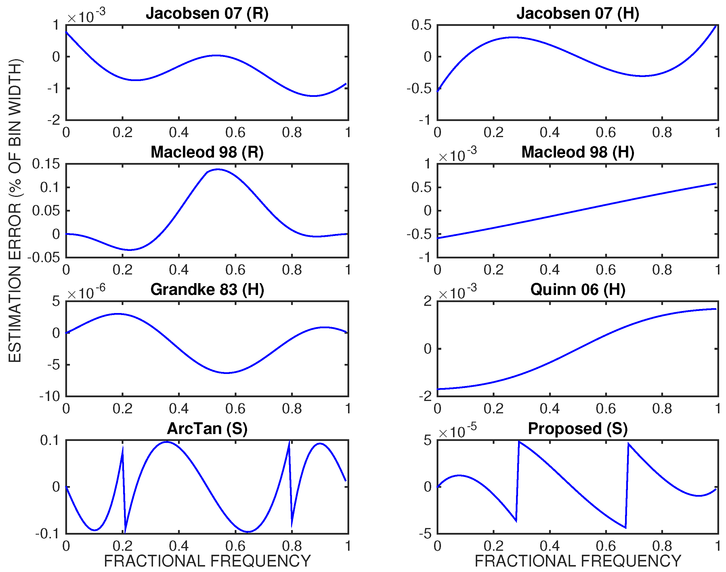Figure 6 represents the deterministic estimation error due to structural bias, as a percent of the DFT bin width, which is associated with eight of the tested frequency estimators in the absence of harmonic and noise interferences, when $N=512$, and when $\mathsf{\ell }=N/4$. It should be noted that this particular value of ℓ corresponds to the ‘sweet spot’ in the sense that, for a real sinusoid, it minimizes self-leakage due to the Dirichlet kernel located on the negative frequency axis. Even though the setting $\mathsf{\ell }=N/4$ is frequently used in the literature to report results, it is not representative of realistic operational conditions with real-world signals.

In Figure 6, we use $\mathsf{\ell }=N/4$ just to give a first flavour of a comparative perspective for different frequency estimators, and also to emphasize that a lower estimation error in Figure 6 is not indicative of a ‘better’ estimator, because the test conditions are not representative of the capability of each estimator to handle noise and leakage due to quasi-harmonic interference. This capability will be more correctly assessed in the following sections using as a reference the performance criterion that is described in Section 2.5, and taking the overall error that reflects structural bias, error variance from the noise, and ‘bias due to multiple tones’ [21].

4.1. Results with No Harmonic Interference

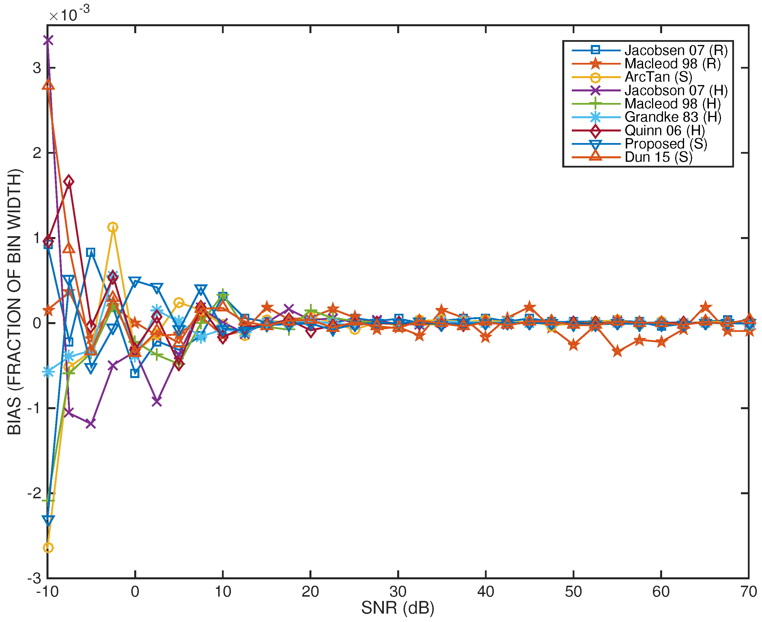
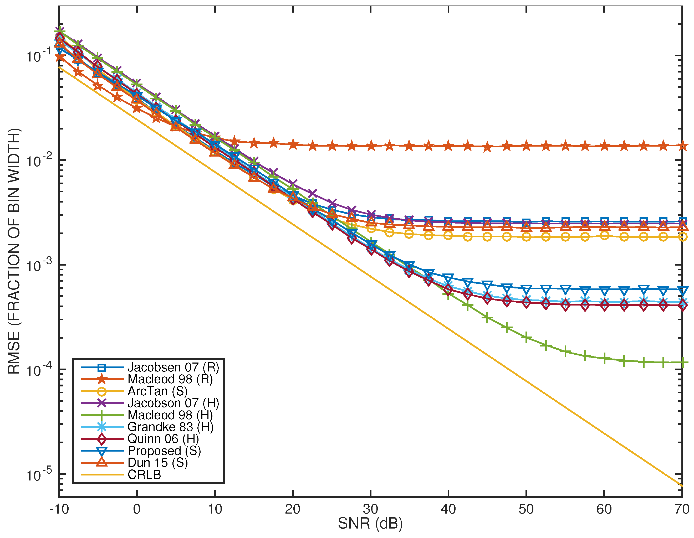
Figure 7 represents the test results regarding systematic bias, i.e., the $\mathrm{mean}\left\{{\omega }_{\mathsf{\ell }}-{\widehat{\omega }}_{\mathsf{\ell }}\right\}$ results, when there is no harmonic interference. The results are normalized by the DFT bin width. Figure 8 represent the test results regarding RMSE according to (13) and in the absence of harmonic interference. Regarding systematic bias, it starts in the range 0.1–0.3% for very low SNR values, and vanishes rapidly for all frequency estimators when the SNR varies between −10 dB and 20 dB. Above 25 dB SNR, the bias can be considered negligible.

Regarding RSME results, four groups of estimators can be identified that have, each, a similar trend in terms of performance. First, as the SNR increases, the Jacobsen07(H) and the Macleod98(R) estimators are the first two to suffer from strong bias due to noise given that, for SNR > 25 dB, their performance saturates above 0.002 (or 0.2% of the DFT bin width). It is remarkable, however, that, below 20 dB SNR, the Macleod98(R) estimator better approaches the CRLB than any other estimator, which makes it the best performing estimator in this SNR range. Three main reasons help to explain this outcome: the rectangular window allows the estimator to benefit from the best frequency selectivity, as the main lobe of the frequency response of the rectangular window is the narrowest, this advantage is more effective when the SNR becomes less than the minimum main-to-side lobe attenuation of the rectangular window, which is around 13 dB, and the estimator uses spectral phase information in addition to spectral magnitude information.

The ArcTan(S) estimator is the next to show an asymptotic behavior since its RMSE performance saturates to around 0.07% of the DFT bin width for SNR > 35 dB. The next two estimators to show a close asymptotic behavior are the Jacobsen07(R) and the Dun15(S) estimators, when SNR > 50 dB. This causes some surprise, because the Jacobsen07(R) uses the rectangular window, which is known to have the poorest main-to-side lobe attenuation. However, the fact that this estimator also uses phase, in addition to spectral magnitude information, and benefits from the improvement introduced by Candan [64], means that its performance exceeds what could be expected at first sight. This result highlights the non-obvious conclusion that a given estimator may possess an intrinsic ability to ‘cancel’ bias, such that it may outperform other estimators that use windows with an improved main-to-side lobe attenuation. Finally, the Quinn06(H), the Macleod98(H), the Grandke83(H), and the Proposed(S) estimators follow a similar trend at an almost constant distance from the CRLB.

The relative behavior between the estimators tested here is consistent with the ‘ranking’ that emerged from our previous research [44].

4.2. Results with Mild Quasi-Harmonic Interference

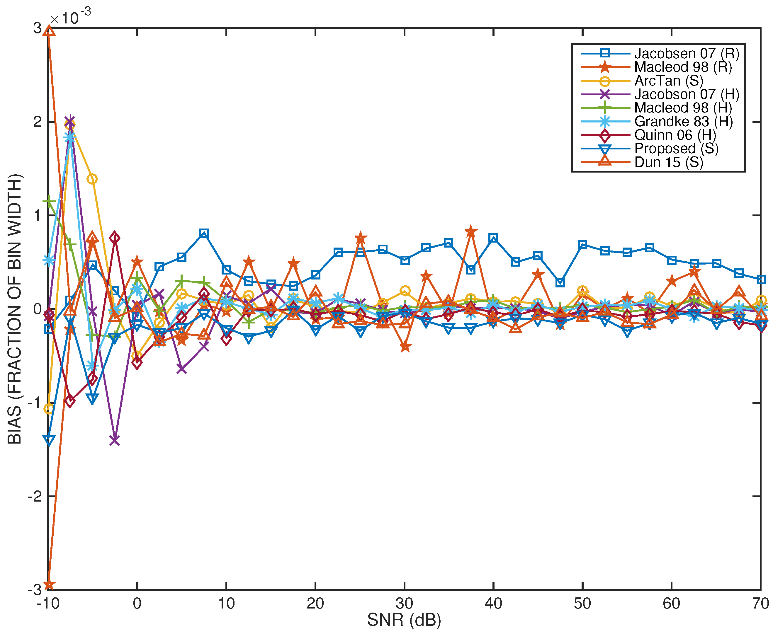
Figure 9 and Figure 10 depict, respectively, the systematic bias and RMSE performance results of all tested frequency estimators when the quasi-harmonic interference, as defined in Section 2.3, is mild. Regarding systematic bias, the trend for all estimators is quite similar to what was observed in the case of absence of quasi-harmonic interference (previous subsection), except for the Macleod98(R) estimator, whose systematic bias level fluctuates even when the SNR is high, although it does not exceed 0.05% of the DFT bin width.

Regarding RMSE, four performance trends can be identified as in the previous case (Section 4.1). The first aspect to note is that these trends reflect a degradation relative to what is observed in Figure 8, in the sense that the asymptotic behavior initiates for lower SNR values. This is expected, given that leakage effects are stronger. The second aspect to highlight and that represents a surprise is that the frequency estimators that share a similar trend are different in Figure 8 and in Figure 10. For example, the RMSE performance of the Macleod98(R) estimator now saturates above 0.01 (or 1% of the DFT bin width) for SNR > 10 dB, which shows that bias effects due to leakage dominate. A second trend collapses the RMSE performances of four estimators that were separated in Figure 8: the Jacobsen07(H) estimator, the ArcTan(S) estimator, and the Jacobsen07(R) and Dun15(S) estimators. A third trend groups the Quinn06(H), the Grandke83(H), and the Proposed(S) estimators, whose RMSE performances saturate around 0.04% of the DFT bin width for SNR > 40 dB. Finally, the Macleod98(H) estimator is able to follow the CRLB more closely for SNR > 40 dB. It is interesting to note that this estimator is one of the two estimators that are more distant from the CRLB for SNR < 20 dB, which suggests that a lower performance at low SNR is compensated by a higher performance at high SNR. This is also the case for the Macleod98(R) estimator, which approaches the CRLB closer than any other estimator when the SNR is less than about 5 dB.

4.3. Results with Strong Quasi-Harmonic Interference

Figure 11 and Figure 12 represent, respectively, the performance results of all tested frequency estimators under strong full-bandwith quasi-harmonic interference, as specified in Section 2.3. As expected, relatively to the previous two test cases, both in terms of systematic bias and RMSE, performance curves exhibit a stronger degradation. Regarding systematic bias, in addition to the remarks already made concerning the previous two test cases, the current test case reveals that the systematic bias is non-negligible for most estimators, even when the SNR exceeds 10 dB, and especially in the case of the two rectangular window-based estimators (i.e., the Jacobsen07(R) and the Macleod98(R) estimators), whose structural bias may be as high as 0.1% of the DFT bin width.

Regarding the RMSE performance curves, as expected, the asymptotic behavior initiates for even lower SNR values, relative to the previous test case. On the other hand, it can be seen that all performance curves collapse to three major trends. The worst-performing trend involves only the Macleod98(R) frequency estimator, whose RMSE performance saturates to around 3.5% of the DFT bin width for SNR > 5 dB. The next best-performing trend groups the Jacobsen07(R), the Dun15(S), and the ArcTan(S) estimators. The best-performing group of frequency estimators includes the Jacobsen07(H), the Proposed(S), the Grandke83(H), the Quinn06(H), and the Macleod98(H) estimators. The RMSE performance of these estimators saturates to around 0.4% of the bin width for SNR > 20 dB.

4.4. Main Conclusions

The results in Section 4.1, Section 4.2 and Section 4.3 suggest several relevant conclusions that are summarized next.

• First, systematic bias affects all frequency estimators in a similar way, varying between 0.1% and 0.3% of the bin width when the SNR is the range −10 dB to +10 dB, and vanishes rapidly for higher SNR, such that it can be considered negligible, except in the case of the Macleod98(R) and Jacobsen07(R) estimators, whose systematic bias can be as high as 0.1% of the DFT bin width under strong quasi-harmonic interference.
• Second, in terms of RMSE, it is clear that more severe quasi-harmonic interference conditions degrade the performance of all frequency estimators, but this degradation is not the same for all estimators. This fact is explained by the intrinsic robustness of each estimator, which depends not only on the window that is associated with the estimator, but also on their estimation approach dealing with spectral magnitude information only, or a combination of spectral magnitude and phase. For example, the Jacobsen07(H) estimator uses spectral magnitude only, and the Macleod98(H) estimator uses both spectral magnitude and phase, which is what gives it an ‘intrinsic leakage rejection’ capability [30].
• Third, the relative performance of the same estimator depends not only on the SNR (as expected), but is also highly influenced by the severity of the quasi-harmonic interference. For example, it is quite interesting to observe that the Jacobsen07(H) estimator is the worst-performing estimator when the test conditions do not involve harmonic interference, it belongs to the second group of worst-performing estimators under mild quasi-harmonic interference, and it belongs to the group of best-performing estimators under strong quasi-harmonic interference. This reflects the fact that all estimators suffer a stronger performance degradation when the test conditions become more severe, but that degradation affects different estimators differently. The Jacobsen07(H) estimator appears to be an exception, as its performance is quite consistent across test cases. Thus, it may be concluded that operational conditions dictate if a given estimator has a better or worse relative performance. For example, the Macleod98(R) estimator exhibits the best relative performance across test cases for very low SNR levels (because it approaches better the CRLB), but exhibits the worst relative performance across test cases for moderate and high SNR levels (because its performance curve saturates to higher RMSE values). Results also suggest that if a given estimator shows a good performance under no harmonic interference, it may perform poorly when subject to strong quasi-harmonic interference. This is the case of the Jacobsen07(R) estimator.
• Fourth, when the quasi-harmonic interference is strong, its impact on the frequency estimation performance for the majority of the estimators considered in this paper is quite significant, which confirms that it has a dominant effect in limiting the performance.
• Finally, our results suggest that when a frequency estimator shows a relative better performance across test cases at high SNR, that is obtained at the cost of a relatively worse performance across test cases at low SNR. That is clearly the case for the Macleod98(H) estimator when harmonic interference is mild or strong.

Finally, it is instructive to relate the absolute estimation error of the different frequency estimators when they operate on the ‘sweet spot’ and in the absence of harmonic interference and noise, as illustrated in Figure 6, and the variance of the estimation error that is associated to the different estimators under the ‘stress test’ that the results in Figure 12 reflect. It is clear that a much smaller absolute estimation error under ideal (i.e., no stress) conditions is not necessarily indicative of a much better performance under a realistic and stressful scenario. That is the case of the Grandke83(H) and the Proposed(S) estimators.

5. Conclusions

In this paper, we compared the relative performance of nine non-iterative, discrete Fourier transform-based (DFT) frequency estimators, taking as a reference the Cramér–Rao Lower Bound (CRLB) for the error variance of a general unbiased estimator, and considering the combined impact of such aspects as spectral selectivity and main-side lobe attenuation of the analysis window, the Signal-to-Noise Ratio (SNR), the algorithmic approach of the estimator dealing with just spectral magnitude information or a combination of spectral magnitude and phase, and, most importantly, the severity of quasi-harmonic interference that includes amplitude modulation and frequency modulation.

The results indicate that quasi-harmonic interference plays a major role in constraining the performance of all frequency estimators, especially when it is strong, in which case the performances of the majority of the tested frequency estimators collapse to just a few trends relative to the CRLB.

The results also indicate that the performance of a given estimator, which includes systematic bias and variance aspects, is not uniquely determined by the characteristics of the window being used by that estimator, nor is it predicted by the maximum absolute estimation error when the frequency of one single sinusoid is estimated in the absence of noise and harmonic interference. Rather, it depends on how well the frequency estimator takes advantage of the frequency response of the window being used by that estimator, and depends on the intrinsic ability of the estimator to ‘cancel’ bias due to multiple tones, which is a feature that seems to benefit from spectral phase information, in addition to magnitude.

Other relevant conclusions emerging from our research include: (i) a rectangular window-based frequency estimator (Macleod98(R)) approaches the CRLB better than any other estimator for low SNR values (e.g., <20 dB under no harmonic interference), (ii) if a frequency estimator shows a higher relative performance at high SNR it tends to show a lower relative performance at low SNR, (iii) quasi-harmonic interference does not degrade the performance of different estimators in a similar way, and (iv) if the severity of quasi-harmonic interference is high, estimators that are based on the Hanning and sine windows show better and similar performances, in the order of 0.4%, relative to the bin width of the DFT filter bank, which means that they can be considered sufficiently accurate for practical purposes when tens or hundreds of concurrent sinusoids need to be analyzed in real time.

Future work will leverage on the most important findings reported here in order to tackle multi-pitch estimation in concurrent speech and singing, as well as music chord identification and separation.