Abstract
This study aimed to establish and verify the validity of an acoustic simulation method during sustained phonation of the Japanese vowels /i/ and /u/. The study participants were six healthy adults. First, vocal tract models were constructed based on computed tomography (CT) data, such as the range from the frontal sinus to the glottis, during sustained phonation of /i/ and /u/. To imitate the trachea, after being virtually extended by 12 cm, cylindrical shapes were then added to the vocal tract models between the tracheal bifurcation and the lower part of the glottis. Next, the boundary element method and the Kirchhoff–Helmholtz integral equation were used for discretization and to represent the wave equation for sound propagation, respectively. As a result, the relative discrimination thresholds of the vowel formant frequencies for /i/ and /u/ against actual voice were 1.1–10.2% and 0.4–9.3% for the first formant and 3.9–7.5% and 5.0–12.5% for the second formant, respectively. In the vocal tract model with nasal coupling, a pole–zero pair was observed at around 500 Hz, and for both /i/ and /u/, a pole–zero pair was observed at around 1000 Hz regardless of the presence or absence of nasal coupling. Therefore, the boundary element method, which produces solutions by analysis of boundary problems rather than three-dimensional aspects, was thought to be effective for simulating the Japanese vowels /i/ and /u/ with high validity for the vocal tract models encompassing a wide range, from the frontal sinuses to the trachea, constructed from CT data obtained during sustained phonation.
1. Introduction
The nasopharyngeal closure function is known to be crucially involved in articulatory disorders that occur after palatoplasty in patients with cleft palate and may also be involved in both the morphology and movement of articulatory organs, including the palate and tongue [1]. However, no method has been devised to assess in detail the association between articulatory disorders and the morphology and movement of articulatory organs; therefore, the pathogenesis remains unclear.
The recent development of acoustic wave-based techniques, such as the finite element, finite difference, and boundary element methods, has made it possible to visualize and conduct a detailed analysis of the relationship between the morphology of, and sound produced by, a three-dimensional (3D) shape obtained for a 3D model of the vocal tract [2,3,4,5,6,7]. Many analysis methods using the finite element method have been reported, but the range targeted for the analysis target has been limited to a small area from the oral cavity to the glottis.
We established a simulation method using computed tomography (CT) data during phonation of /a/ in order to clarify the relationship between the morphology of the articulatory organs and the sounds produced by applying the boundary element method. We thereby aimed to elucidate the causes of abnormal articulation, and to propose and develop treatment methods. By applying the FMBEM (fast multipole boundary element method) for analysis [8], which produces solutions by analyzing boundary problems instead of three-dimensional aspects in a previous study, we demonstrated that it enables fast analysis for models covering a wide range of areas. Therefore, we were able to use a model of a wide range of areas including the paranasal sinuses, oral cavity, pharynx, larynx, and airway. The model was validated and found to be able to perform simulations with sufficient accuracy [9].
Consequently, the present study was conducted to establish a simulation method for the other vowels. As compared with the wide vowel /a/, /i/ and /u/ are narrow vowels, and the volume of the oral cavity in the vocal tract model is small. Therefore, we aimed to establish a simulation of the narrow vowels. Furthermore, in the present study, the two vowels, /i/ (narrow front) and /u/ (narrow rear vowels), which differ in the site of the oral cavity, which is narrowed, were targeted for analysis, and we then performed simulations with the same parameters as for the vowel /a/. The validity of the model was verified using frequency analysis obtained from an actual voice.
2. Materials and Methods
2.1. Participants
The study participants were six healthy adults (three males, three females; age range, 26–45 years) with a normal occlusal relationship and no abnormalities in the articulatory organs. The Institutional Review Board of Yamaguchi University Hospital approved this study (H26-22-4), and written, informed consent was obtained from all participants.
2.2. Simulation Method
The CT imaging (SOMATOM Force; Siemens Healthineers, Munich, Germany) was carried out with a tube voltage of 100 (+Tin filer) kV, a tube current of 96 mA, slice thickness of 0.6 mm, CT dose index volume of 0.23 mGy, and exposure dose of 0.1 mSv. All CT data were obtained during sustained phonation of the Japanese vowels /i/ and /u/ while the participants were in the supine position. In total, the scanning time was 5 s from the upper end of the frontal sinus to the supraclavicular region.
Following visualization of the CT scan data, a 3D model was constructed using Amira 3D visualization software (version 5.6.0; Maxnet, Tokyo, Japan). Next, to construct a vocal tract model, we manually extracted the airways to the frontal, ethmoid, sphenoid, and maxillary sinuses, the nasal and oral cavities, and the pharynx, larynx, and glottis from the CT data segments on the coronal, axial, and sagittal sections. These data were then saved in the STL file format. Next, we extended the virtual cylindrical structure by 12 cm from the lower part of the glottis to the tracheal bifurcation to reduce the exposure dose (Figure 1). Then, based on the simulation results, the length of the extension was adjusted by 1–2 cm.
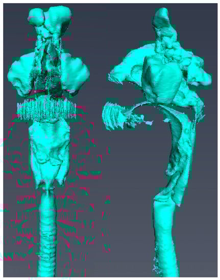
Figure 1.
Vocal tract model.
- A vocal tract model including the frontal sinus, ethmoid sinus, sphenoid sinus, maxillary sinus, nasal cavity, oral cavity, pharynx, larynx, and glottis is shown.
To conduct acoustic analysis, we created a mesh model from the vocal tract model using the boundary element method. To equalize and adjust the mesh size and remove unnecessary meshes, a direct modeler (Ansys SpaceClaim, version 2021R1; ANSYS, Canonsburg, PA, USA) was used to modify the vocal tract model, after which the meshes of the nostril and oral aperture were removed. Next, the nasal and oral cavities and tracheal bifurcation were opened. To aid the mesh creation, we applied triangular elements (smallest mesh size, 2 mm) and carried out the analysis on a Dell Precision T3610 workstation (Inter Xeon E-1650 3.5 GHz) with the WAON software package (version 4.55; Cybernet, Tokyo, Japan) (Figure 2). We used mesh sizes of 19.6 and 39.2 mm for /i/ and /u/, respectively, based on a previous study [10] that recommended a mesh size smaller than 1/6 of the wavelength of the sound wave of the analysis frequency for a body temperature of 37 °C (speed of sound, 352.85 m/s). For the creation of a vocal tract model that did not include the nasal cavity and sinuses, these were separated at the section in which a cross-sectional area of the nasal coupling was minimized.
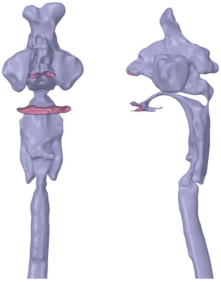
Figure 2.
Mesh model for simulation.
- A surface mesh model for analysis is shown. The nostrils, oral cavity, and tracheal bifurcation are opened.
Acoustic analysis was performed at a range from 1 to 3000 Hz for /i/ and from 1 to 1500 Hz for /u/ at 1 Hz intervals using WAON (Cybernet). Next, the boundary element method and the Kirchhoff–Helmholtz integral equation were used for discretization and to represent the wave equation for sound propagation, respectively, the details of which have been described elsewhere [9].
The wall of the vocal tract model was regarded as rigid, so the sound absorption coefficient was set to 0% with a specific acoustic impedance of ∞. Conversely, the bottom of the virtual trachea was regarded as nonrigid after being extended cylindrically between the tracheal bifurcation and the lower part of the glottis [11]. Assuming a constant body temperature, the acoustic medium was set to 37 °C; at this temperature, the sound velocity was 352.85 m/s and the density was 1.1468 kg/m3. The sound source and observation point were set as points in a place corresponding to the vocal cords and a location 10 cm in front of the lips, respectively. A frequency response curve was then drawn at the sound pressure level to calculate the first formant (F1) and second formant (F2).
2.3. Validity of the Acoustic Simulation
Similar to the CT scanning, the Japanese vowels /i/ and /u/ (each sustained for 5 s) were recorded through a dynamic vocal microphone (SHURE SM58; Niles, IL, USA) placed approximately 10 cm in front of the participants’ lips using a solid-state audio recorder (Marantz Professional PMD661; inMusic Brands, Cumberland, RI, USA). All recordings were obtained in a soundproof room while the participants were in the supine position.
The recorded voice data (sampling rate, 44.1 kHz) were saved on an SD memory card (16 bits) in the .wav file format. After down-sampling the voice data from 44.1 to 11.025 kHz, F1 and F2 were calculated using Multi Speech 3700 acoustic analysis software (PENTAX Medical, Montvale, NJ, USA).
The vowel formant frequency discrimination thresholds for American English and Japanese, which have been reported to be under 3–5% [12] and 4.9–9.6% [13], respectively, were used in the present study to evaluate validity. The validity was considered acceptable if these criteria were met. The relative discrimination threshold (%) was obtained by dividing ΔF by F, where F is the formant frequency calculated from the simulation, and the discrimination threshold ΔF is the difference between F and the formant frequencies of the actual and artificial voices generated from the solid models [13].
3. Results
The vocal tract model acoustic simulation results are shown in Table 1 and Table 2. The formant frequencies obtained from all participants in the simulation were within the F1 and F2 frequency ranges previously reported for the vowels /i/ and /u/ [14]. For F1 and F2, the relative discrimination thresholds of the vowel formant frequencies against actual voice ranged from 1.1% to 10.2% and from 3.9% to 7.5% for /i/, and from 0.4% to 9.3% and from 5.0% to 12.5% for /u/, respectively. Several thresholds exceeded 9%, but the relative discrimination thresholds became 9% or less by shortening the virtual cylindrical trachea. Specifically, the relative discrimination thresholds became 7.8% for F1 of /i/ in subject No. 6, 0.6% for F2 of /u/ in subject No. 3 by shortening by 1 cm, and 2.4% for F2 of /u/ in subject No. 2 by shortening by 2 cm.

Table 1.
Details of simulated formant frequencies from a vocal tract model calculated from the actual voice of /i/.
Table 2.
Details of simulated formant frequencies from a vocal tract model calculated from the actual voice of /u/.
The acoustic simulation results for various extension lengths of the virtual trachea are shown in Table 3 and Table 4. As the length of the virtual trachea shortened, the formant frequencies increased, except for F1 of /i/ in subject No. 1. The standard deviations of F1 and F2 obtained by the acoustic simulation were 2.9–22.1 cm and 43.7–135.2 cm for /i/, and 4.7–31.0 cm and 20.2–101.3 cm for /u/, respectively, when the lengths of the virtual trachea were changed to 10 cm, 11 cm, and 12 cm. The standard deviations with the changes in extension lengths varied considerably.
Table 3.
Formant frequencies simulated for /i/ by various extension lengths of the virtual trachea (Hz).
Table 4.
Formant frequencies simulated for /u/ by various extension lengths of the virtual trachea (Hz).
Three of the six participants had a connection to the nasal cavity at the nasopharynx (i.e., nasal coupling), whereas the remaining three did not (Table 5). The minimum cross-sectional areas at the nasal coupling for the three participants with nasal coupling are shown in Table 5. The average cross-sectional areas of /i/ and /u/ were 1.57 and 8.01 mm2, respectively.
Table 5.
Minimum cross-sectional area at the nasal coupling for /i/ and /u/ (mm2).
The typical frequency response curves obtained by the acoustic simulation are shown in Figure 3, Figure 4, Figure 5 and Figure 6. A peak around 500 Hz was observed for /i/ in subject No. 4 and /u/ in subject No. 1, both of whom had nasal coupling (Figure 3 and Figure 4). Conversely, no peaks around 500 Hz were observed for both /i/ and /u/ in the curves obtained for the models without nasal coupling and with nasal coupling but with the nasal cavity and sinuses removed (Figure 5 and Figure 6). Therefore, the peak around 500 Hz was considered to be the pole–zero pair because of the nasal coupling (Figure 3 and Figure 4). Pole–zero pairs around 500 Hz caused by nasal coupling were observed between F1 and F2 for both /i/ and /u/ (Table 6). A further peak was observed at 1000 Hz for /i/ for all participants (Table 6). The peaks around 1000 Hz were observed in the curves obtained for both models of /i/ without nasal coupling and with nasal coupling but with the nasal cavity and sinuses removed (Figure 3 and Figure 5).
Table 6.
Pole–zero pairs for /i/ and /u/.
Comparing the frequency response curves obtained for the models with nasal coupling and those with the nasal cavity and sinuses removed, the frequencies of F1 for /i/ shifted to the low frequency side, whereas those for /u/ shifted to the high frequency side (Figure 3 and Figure 4).

Figure 3.
Frequency response curve for /i/ in subject No. 4.
- The simulation result of the model including the nasal cavity and sinuses is indicated by the solid line, and that of the model excluding the nasal cavity and sinuses is indicated by the dotted line. In the former curve, the first peak is F1 (374 Hz), the second is due to nasal coupling for a pole–zero pair (pole: 406 Hz; zero: 486 Hz), the third is a pole–zero pair (pole: 1206 Hz; zero: 1240 Hz), and the fourth is F2 (2510 Hz). In the latter curve, the first peak is F1 (319 Hz), the second is not due to nasal coupling for a pole–zero pair (pole: 1202 Hz; zero: 1242 Hz), and the third is F2 (2509 Hz).

Figure 4.
Frequency response curve for /u/ in subject No. 1.
- The simulation result of the model including the nasal cavity and sinuses is indicated by the solid line, and that of the model not including the nasal cavity and sinuses by the dotted line. In the former curve, the first peak is F1 (371 Hz), the second is due to nasal coupling for a pole–zero pair (pole: 462 Hz; zero: 492 Hz), and the third is F2 (1127 Hz). In the latter curve, the first peak is F1 (409 Hz) and the second is F2 (1111 Hz).

Figure 5.
Frequency response curve for /i/ in subject No. 2.
- The frequency response curve obtained from the simulation of the models without the nasal cavity and sinuses is shown. The first peak is F1 (365 Hz), the second is a pole–zero pair (pole: 944 Hz, zero: 1175 Hz) not due to nasal coupling, and the third is F2 (2204 Hz).

Figure 6.
Frequency response curve for /u/ in subject No. 5.
- The frequency response curve obtained from the simulation of the models without the nasal cavity and sinuses is shown. The first peak is F1 (495 Hz) and the second is F2 (1220 Hz).
4. Discussion
By using the boundary element method in the same way as for the Japanese vowel /a/ and applying the same parameter settings [9], an acoustic simulation could be stably performed for the Japanese vowels /i/ and /u/. In a previous study [14], F1 and F2 of /i/ ranged from 250 to 500 Hz and from 2000 to 3000 Hz, respectively, and those of /u/ ranged from 300 to 500 Hz and from 1000 to 2000 Hz, respectively; the formant frequencies obtained from the present simulation were almost within these ranges.
Similar to the analysis of the Japanese vowel /a/, CT imaging was performed. The CT scanner we used had the advantage of being able to minimize the exposure dose. Conventional chest CT examinations produce a radiation exposure dose of 5–30 mSv, whereas the CT scanner used in the present analysis only exposed patients to a radiation dose of 0.1 mSv, which is a level comparable to that of a general chest X-ray [15].
A previous study that conducted a sound analysis of the Japanese vowel /a/ [9] set the sound source as a point in a place corresponding to the vocal cords, modified the sound by reflection, absorption, and interference on the wall of the vocal tract, and used the boundary element method to analyze the sound that radiated from the mouth and nostrils to the outside space. As compared with the Japanese vowel /a/, /i/ and /u/ are narrow vowels, and the volume of the oral cavity is slightly narrower, but not extremely so. Therefore, we considered that it could be simulated by using the same boundary element method with the same parameter settings, that is, the wall of the vocal tract and the bottom end of the virtual trachea were regarded as rigid and very soft walls, respectively, and the sound velocity and density were set at 37 °C.
In the verification using actual voice, the relative discrimination thresholds were within 9%, except for one of the six cases for F1 of /i/ and two of the six cases for F2 of /u/. No significant difference was found between the numbers of participants in whom the relative discrimination thresholds were 9% or less in the present simulations of /i/ and /u/ or the previous simulation of /a/ [9]. Similar to the results of the previous simulation of /a/, adjusting the length of the virtual cylindrical extension of the lower part of the glottis resulted in relative discrimination thresholds of less than 9%. In the present study, as the length of the virtual trachea shortened, the formant frequency increased, except for F1 of /i/ in subject No. 1. However, discussing the appropriate length of the virtual trachea exceeds the scope of the present study.
In the present acoustic simulation, the use of the boundary element method to obtain the frequency response resulted in peaks other than the formant frequencies. Chen [16] reported that peaks arising from nasalization are often observed at a position lower than F1 or between F1 and F2 in narrow vowels with a high tongue position. In the present study, peaks were observed between F1 and F2 for /i/ and /u/ (Table 6). Because the Japanese vowels /i/ and /u/ are narrow vowels, our results were consistent with those reported by Chen [16]. Peaks around 500 Hz have been observed for vowels [17]. Because a peak around 500 Hz is not observed in vocal tract models without a nasal cavity, the peak, i.e., the pole–zero pair, is considered to arise from the nasal coupling of vowels [17].
It is also known that a pole–zero pair appears at around 500 Hz because of nasal coupling, and that the presence of a pole–zero pair changes the position where the peak of F1 appears in the frequency response curves [17]. In the present study, among three participants with nasal coupling, the obtained peaks of F1 shifted to the low frequency side in two participants for /i/ and to the high frequency side in three for /u/ in the simulated vocal tract models in which the nasal cavity and sinuses had been removed.
Resonance in the paranasal cavities has been reported to generate pole–zero pairs that are not the result of nasal coupling, leading to more complex frequency response curves [18]. In the present simulation of the Japanese vowel /i/, two peaks appearing at around 500 and 1000 Hz were observed between F1 and F2. The peak at around 500 Hz was considered to be the pole–zero pair due to nasal coupling. The other peak at a higher frequency occurred at around 1000 Hz in /i/ for all participants. No gender difference in the occurrence of the peaks was observed. Because a peak was observed at 1000 Hz regardless of the presence of the nasal cavity, the peaks were considered to have been generated on either site of the vocal tract, excluding the nasal coupling. However, further discussion exceeds the limitations of the present study.
5. Conclusions
The findings of the present study using the boundary element method demonstrated that sound propagation and emission during sustained phonation of the Japanese vowels /i/ and /u/ and virtual cylindrical extension from the lower part of the glottis could be simulated well in a vocal tract model that included the range from the frontal sinus to the glottis. A comparison with actual voice confirmed the validity of the simulation. This proposed method is an acoustic analysis that can be applied only to the sounds that have a sound source in the vocal cords and do not involve extreme narrowing of the vocal tract. For other articulations, it is necessary to develop a novel simulation method.
Author Contributions
Conceptualization, K.M.; methodology, K.M.; software, M.T. and M.M.; validation, M.S. and H.U.; formal Analysis, M.S., M.T., and M.M.; investigation, M.S., M.T., M.M. and H.U.; resources, M.T. and M.M.; data curation, M.S.; writing—original draft preparation, M.S. and K.M.; writing—review and editing, M.S. and K.M.; visualization, M.S. and K.M.; supervision, K.M.; project administration, K.M.; funding acquisition, K.M. All authors have read and agreed to the published version of the manuscript.
Funding
This research was supported by the Japan Society for the Promotion of Science under Grants-in-Aid for Scientific Research (Basic Research (B) 18H03001) and the Kawai Foundation for Sound, Technology, and Music.
Institutional Review Board Statement
The Institutional Review Board of Yamaguchi University Hospital approved this study (H26-22-4), and written, informed consent was obtained from all participants.
Data Availability Statement
Not applicable. There is no dataset associated with this manuscript.
Conflicts of Interest
The authors declare no conflict of interest.
References
- Bejdová, S.; Krajíček, V.; Peterka, M. Variability in palatal shape and size in patients with bilateral complete cleft lip and palate assessed using dense surface model construction and 3D geometric morphometrics. J. Craniomaxillofac. Surg. 2012, 40, 201–208. [Google Scholar] [CrossRef] [PubMed]
- Fleischer, M.; Rummel, S.; Stritt, F.; Fischer, J.; Bock, M.; Echternach, M.; Richter, B.; Traser, L. Voice efficiency for different voice qualities combining experimentally derived sound signals and numerical modeling of the vocal tract. Front. Physiol. 2022, 13, 1081622. [Google Scholar] [CrossRef] [PubMed]
- Dabbaghchian, S.; Arnela, M.; Engwall, O.; Guasch, O. Simulation of vowel-vowel utterances using a 3D biomechanical-acoustic model. Int. J. Numer. Method Biomed. Eng. 2021, 37, e3407. [Google Scholar] [CrossRef] [PubMed]
- Marc, A.; Rémi, B.; Saeed, D.; Oriol, G.; Francesc, A.; Xavier, P.; Annemie, V.H.; Olov, E. Influence of lips on the production of vowels based on finite element simulations and experiments. J. Acoust. Soc. Am. 2016, 139, 2852–2859. [Google Scholar]
- Takemoto, H.; Mokhtari, P.; Kitamura, T. Acoustic analysis of the vocal tract during vowel production by finite-difference time-domain method. J. Acoust. Soc. Am. 2010, 128, 3724–3738. [Google Scholar] [CrossRef] [PubMed]
- Tsuji, T.; Tsuchiya, T.; Kagawa, Y. Finite element and boundary element modelling for the acoustic wave transmission in mean flow medium. J. Sound Vib. 2002, 255, 849–866. [Google Scholar] [CrossRef]
- Amelia, J.G.; Helena, D.; Damian, T.M. Diphthong synthesis using the dynamic 3d digital waveguide mesh. IEEE/ACM Trans. Audio Speech Lang Process. 2018, 26, 243–255. [Google Scholar]
- Sakuma, T.; Yasuda, Y. Fast multipole boundary element method for large-scale steady-state sound field analysis. Part I: Setup and validation, Acust. Acta Acust. 2002, 88, 513–525. [Google Scholar]
- Shiraishi, M.; Mishima, K.; Umeda, H. Development of an Acoustic Simulation Method during Phonation of the Japanese Vowel/a/by the Boundary Element Method. J. Voice 2021, 35, 530–544. [Google Scholar] [CrossRef] [PubMed]
- Steffen, M. Six boundary elements per wavelength: Is that enough? J. Comput. Acoust. 2002, 10, 25–51. [Google Scholar]
- Zwikker, C.; Kosten, C.W. Sound Absorbent Material; Elsevier: New York, NY, USA, 1949; pp. 1–22. [Google Scholar]
- Lyzenga, J.; Horst, J.W. Frequency discrimination of bandlimited harmonic complexes related to vowel formants. J. Acoust. Soc. Am. 1995, 98, 1943–1955. [Google Scholar] [CrossRef]
- Eguchi, S. Difference limens for the formant frequencies: Normal adult values and their development in children. J. Am. Audiol. Soc. 1976, 1, 145–149. [Google Scholar]
- Hirahara, T.; Akahane-Yamada, R. Acoustic characteristics of Japanese vowels. In Proceedings of the 18th International Congress on Acoustics, Kyoto, Japan, 4–9 April 2004; pp. 3287–3290. [Google Scholar]
- Hosono, M. National Diagnostic Reference Levels in Japan (2020)—Japan DRLs 2020. Available online: http://www.radher.jp/J-RIME/report/DRL2020_Engver.pdf (accessed on 22 May 2023).
- Chen, M.Y. Acoustic correlates of English and French nasalized vowels. J. Acoust. Soc. Am. 1997, 102, 2360–2370. [Google Scholar] [CrossRef] [PubMed]
- Kenneth, N.S. Acoustic Phonetics; MIT Press: Cambridge, MA, USA, 2000; pp. 135–137. [Google Scholar]
- Havel, M.; Kornes, T.; Weitzberg, E.; Lundberg, J.O.; Sundberg, J. Eliminating paranasal sinus resonance and its effects on acoustic properties of the nasal tract. Logoped. Phoniatr. Vocol. 2016, 41, 33–40. [Google Scholar] [CrossRef] [PubMed]
Disclaimer/Publisher’s Note: The statements, opinions and data contained in all publications are solely those of the individual author(s) and contributor(s) and not of MDPI and/or the editor(s). MDPI and/or the editor(s) disclaim responsibility for any injury to people or property resulting from any ideas, methods, instructions or products referred to in the content. |
© 2023 by the authors. Licensee MDPI, Basel, Switzerland. This article is an open access article distributed under the terms and conditions of the Creative Commons Attribution (CC BY) license (https://creativecommons.org/licenses/by/4.0/).