A Modification of the Monte Carlo Filtering Approach for Correcting Negative SEA Loss Factors

Abstract

Monte Carlo Filtering (MCF) is one of the methods of Experimental Statistical Energy Analysis (E-SEA), which allows the correction of negative LFs (Loss Factors). In this article, a modification of the MCF method, called DESA (Diagonal Expansion of the Search Area), is proposed. The technique applies a non-uniform extension of the search area when generating a population of normalized energy matrices. The degree of expansion of the search area is controlled by the Diagonal Penalty Factor (DPF). The authors demonstrated the method’s effectiveness on a system that could not be identified in several frequency bands by the classical MCF method. After applying DESA, it was possible to fill in the problematic bands that were missing CLF (coupling loss factor) and DLF (damping loss factor) values. The paper also proposes a way to minimize the errors introduced by using overly high DPF values.

1. Introduction

Statistical Energy Analysis (SEA) is a numerical method for conducting vibroacoustic energy flow analyses in complex systems in the high-frequency range, including predictions of the acoustic power radiated by complex structures [1]. The idea of the SEA method is to divide a structure into so-called subsystems and write down the energy balance between these subsystems in the form of a set of linear equations. The parameters describing the SEA model are the Loss Factors (LF, Loss Factors), divided into the Coupling Loss Factor (CLF), which describes the energy flowing between the subsystems, and the Damping Loss Factor (DLF), which describes the internal losses of the individual subsystems. The SEA model, based on the known excitation powers of each subsystem, gives the spatially, frequency, and time domain averaged energies describing the individual subsystems as output. From the determined energies, it is then easy to convert them to quantities directly used in engineering: the average velocities present in the mechanical subsystem and the average acoustic pressure in the acoustic subsystem. SEA is used in many industries where vibration and noise transmission reduction plays a key role [2,3,4].

Parallel to the predictive SEA method, its experimental counterpart, Experimental SEA (E-SEA), was being developed. E-SEA focuses on issues of measuring loss factors. Bies and Hamid were the first to put into practice a method known as PIM (Power Injection Method) derived directly from the SEA energy balance [5]. PIM allows both CLF and DLF factors of a structure to be determined experimentally without having to disassemble individual system components.

Damping loss factor (DLF) coefficients can also be determined by analyzing the decay curve determined from the impulse response (see, for example [6]). Bloss et al. compared those two methods for determining DLF coefficients and showed good agreement between them when using a sufficiently large number of measurement points in the PIM method [7].

Fahy et al. developed a method for measuring LF coefficients that does not require input power measurement, called IPMT (Input Power Modulation Technique) [8]. In the IPMT method, it is necessary to measure only one receiving point per subsystem, which is its main advantage. IPMT was derived only for the special case of two coupled subsystems and requires the use of specially modulated excitation signals. Another family of methods that do not require input power measurement called ERM (Energy Ratio Method) has also been developed, where it is necessary to know the energy ratios of the individual subsystems during the calculation [9,10,11,12].

Fahy introduced new alternative coefficients to CLF and DLF called power transfer coefficient (PTC) and power dissipation coefficient (PDC) and proposed a way to measure them [13]. The advantage of the method is that there is no need to measure the input power, and there is a better interpretation and physical sense of the defined coefficients. Ming compared the method proposed by Fahy with the PIM measurements and showed that the results from both methods converge for modal overlap conditions greater than unity ($\mu >1$) [14].

Ming also proposed a method for approximating the value of loss factors by measuring the intensity in the structures under study [15]. He showed that the error of the method decreases with increasing the frequency and is negligible when the $\mu$ factor of the receiving subsystem is smaller than the $\mu$ factor of the transmitting subsystem.

Cacciolati et al. developed a methodology for determining loss factors from mechanical admittance measurements [16]. The method is applicable only to point-to-point connections and requires disassembling the system into its components to access the connection points between subsystems.

During PIM measurements, an energy matrix is constructed, and from the matrix that is its inverse, loss coefficients can be extracted. The energy matrix is sensitive to measurement errors, and its inversion can result in the determination of negative loss factors, which have no physical interpretation and are considered measurement errors [17]. The described problem limited the practical applicability of the PIM method, so many research groups were engaged in developing methods to correct negative loss factors.

Lalor proposed breaking the system of E-SEA equations into two independent parts allowing to determine the DLF and CLF coefficients separately [18]. The method reduces the size of the used matrices and improves their condition number. However, there is no guarantee that the method will provide full correction of negative loss factors.

De las Heras et al. proposed a technique called MCF (Monte Carlo Filtering) [19]. MCF involves generating a population of energy matrices based on the matrix obtained from measurements and discarding from the calculation those samples that do not meet the imposed constraints. The authors compared their technique to other methods with a similar philosophy of operation. They showed that the method of residue minimization [20] and the method of Lagrange multipliers [21] provide results at the boundary of the set of admissible solutions, which results in obtaining extreme values after applying these procedures (zeroing of loss factors). The superiority of the MCF method was also demonstrated against the matrix fitting method based on mean-square minimization [22], where loss factors far from the correct values and close to zero were also obtained for some frequency bands. The MCF method is a simulation of a multiply repeated measurement process. It provides results that are inside the set of correct solutions (close to the correct values) and is the most comprehensive method (it lacks additional assumptions, such as weak coupling, no intermediate coupling, and a limited number of subsystems).

The MCF authors validated their method on two systems that met the SEA assumptions. System 1 was virtually generated and consisted of seven subsystems (acoustic interior surrounded by six walls), whereas system 2 was real and consisted of a plate suspended in the acoustic interior (two subsystems) [19]. However, real systems (non-virtual) with more than two subsystems have not been experimentally tested, and the effectiveness of the MCF method for such systems is unknown. In this paper, we analyze this case using an example of a system composed of two steel beams where wave scattering occurs. Thus, the system consisted of four subsystems (flexural wave fields of beams 1 and 2, longitudinal wave fields of beams 1 and 2). The analyzed system proved to be impossible to fully identify by standard methods, which was the motivation for developing a modification of the MCF method described in this paper.

As pointed out before, SEA is based on solving the energy balance between interconnected subsystems:

$$\underset{\_}{P}=\omega \left[L\right]\underset{\_}{E}$$

(1)

where $\underset{\_}{P}$ is a column vector of input powers, $\underset{\_}{E}$ is a column vector of a (unknown) subsystem’s energies, $\omega$ is the center angular frequency of the analyzed band $\mathsf{\Delta }\omega$ (i.e., octave or 1/3-octave band), $\mathrm{and} \left[L\right]$ is the loss factor matrix.

The basic parameters describing the SEA model are the LFs (Loss Factors) ${\eta }_{ij}$, which in turn form the following loss factor matrix $\left[L\right]$ [1].

$$L_{ij}=\left\{\begin{array}{c}{{\displaystyle \sum }}_{u=1}^N{\eta }_{iu}\\ -{\eta }_{ji}\end{array}\right. \begin{array}{c}if i=j\\ if i\ne j\end{array}$$

(2)

where $i=1,\dots N$, $j=1,\dots N$.

The loss factor matrix $\left[L\right]$ can be determined experimentally from the relationship [5]

$$\left[L\right]=\left[P\right] {[E]}^{-1}/\omega$$

(3)

where $\left[P\right]$ is the input power matrix, $\left[E\right]$ is the energy matrix, $\mathrm{and} \omega$ is the angular frequency. $\left[E\right]$ matrix entries $E_{ij}$ stands for the energy of subsystem $i$ when subsystem $j$ is excited. $\left[P\right]$ is a diagonal matrix with entries $P_{jj}$, which stands for the power injected into subsystem $j$. More details about this well-known method, called the Power Injection Method (PIM), can be obtained from other publications [17,23]. The energy matrix can be normalized against input power and angular frequency [24].

$$\left[G\right]=\omega \left[E\right] {\left[P\right]}^{-1}$$

(4)

$\left[L\right]$ is then equal to the inverse of $\left[G\right]$.

$$\left[L\right]={\left[G\right]}^{-1}$$

(5)

The experimentally derived $\left[L\right]$ matrix may contain negative LF coefficients, which have no physical interpretation and which are considered as a measurement error associated with the high sensitivity of ${\left[G\right]}^{-1}$ to measurement uncertainties [17]. To correct the error of negative LFs, the Monte Carlo Filtering (MCF) method can be used [19]. In the MCF method, the essential step is to produce N matrices $\left[G_s\right]$ comprising the population. The subscript “s” comes from the word “sample,” which indicates that the matrix represents a single sample from the population. Creating a $\left[G_s\right]$ matrix involves adding a random increment $\mathsf{\Delta }{G}_{s, ij}$ to each element $G_{ij}$ of the original (derived from measurements) matrix $\left[G\right]$. If we assume that the increments $\mathsf{\Delta }{G}_{s,ij}$ are collected in the pooled matrix $\left[\mathsf{\Delta }{G}_s\right]$, the formula for $\left[G_s\right]$ can be written as

$$\left[G_s\right]=\left[G\right]+\left[\mathsf{\Delta }{G}_s\right]$$

(6)

For clarity, in the rest of the text, we will omit the subscript “s” in the $\left[\mathsf{\Delta }{G}_s\right]$ matrix. The $N$ matrices $\left[G_s\right]$ generated according to (6) compose a set $\left\{\left[G_s\right]\right\}$, which is a Monte Carlo population of normalized energy matrices. The set $\left\{\left[G_s\right]\right\}$ can be written as the sum of two disjoint subsets:

$$\left\{\left[G_s\right]\right\}=\left\{\left[G_s^N\right]\right\}\cup \left\{\left[G_s^P\right]\right\}$$

(7)

where $\left\{\left[G_s^N\right]\right\}$ is the set of energy matrices, the inverses of which $\left\{\left[L_s^N\right]\right\}$ are not correct loss matrices, while $\left\{\left[G_s^P\right]\right\}$ is the set of energy matrices, the inverses of which $\left\{\left[L_s^P\right]\right\}$ are correct loss matrices.

Monte Carlo filtering (MCF) involves excluding $\left\{\left[L_s^N\right]\right\}$ from the calculation and determining the average value of the loss factors based on $\left\{\left[L_s^P\right]\right\}$ only [19]. The selection is performed by inverting $\left[G_s\right]$ and checking if the resulting matrix $\left[L_s\right]$ meets the following conditions:

• All elements off the main diagonal are negative.
• Elements on the main diagonal are positive and greater than the sum of the absolute values of the remaining elements for a given column.

The matrices that satisfy these conditions are positive definite and diagonally dominant. The increment matrix $\left[\mathsf{\Delta }G\right]$ should be based on the measurement uncertainty associated with the experiment, which ensures the generation of $\left[G_s\right]$ in the immediate vicinity of the original matrix $\left[G\right]$. A pooled matrix $\left[\sigma \right]$ is then introduced, where the element ${\sigma }_{ij}$ denotes the standard deviation for the element $G_{ij}$. A matrix $\left[a\right]$ of independent random variables $a_{ij}$ with distribution N (0,1) is also introduced. Then, the matrix of energy increments can be determined from the relation

$$\left[\mathsf{\Delta }G\right]=\left[a\right] \circ \left[\sigma \right]$$

(8)

where ∘ stands for element-wise multiplication (Hadamard product) [25].

The main contributions of the following paper are as follows:

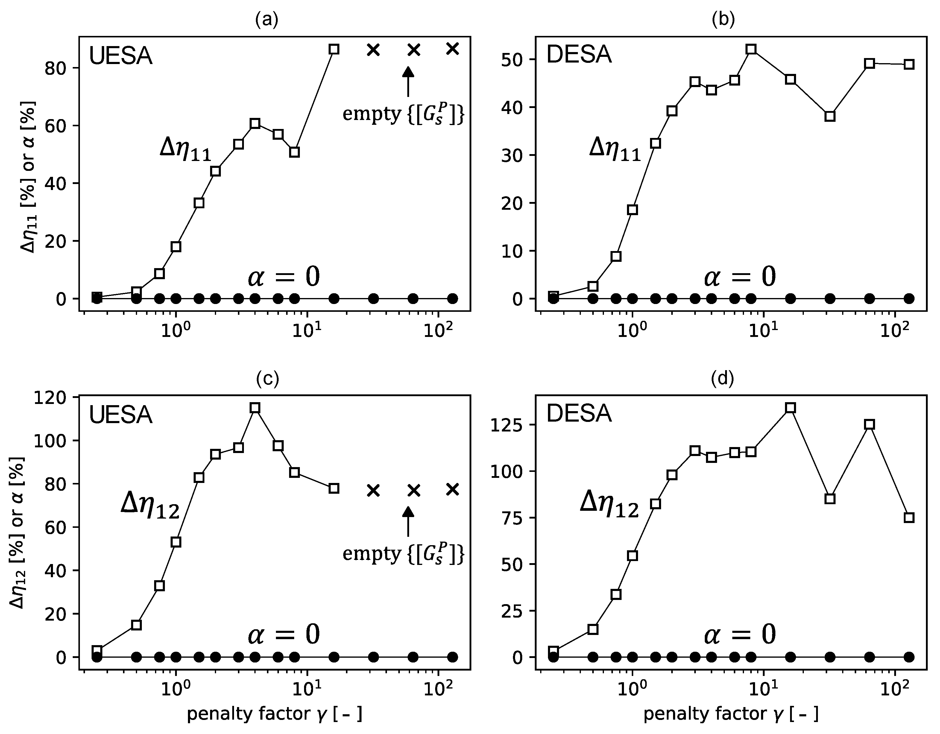
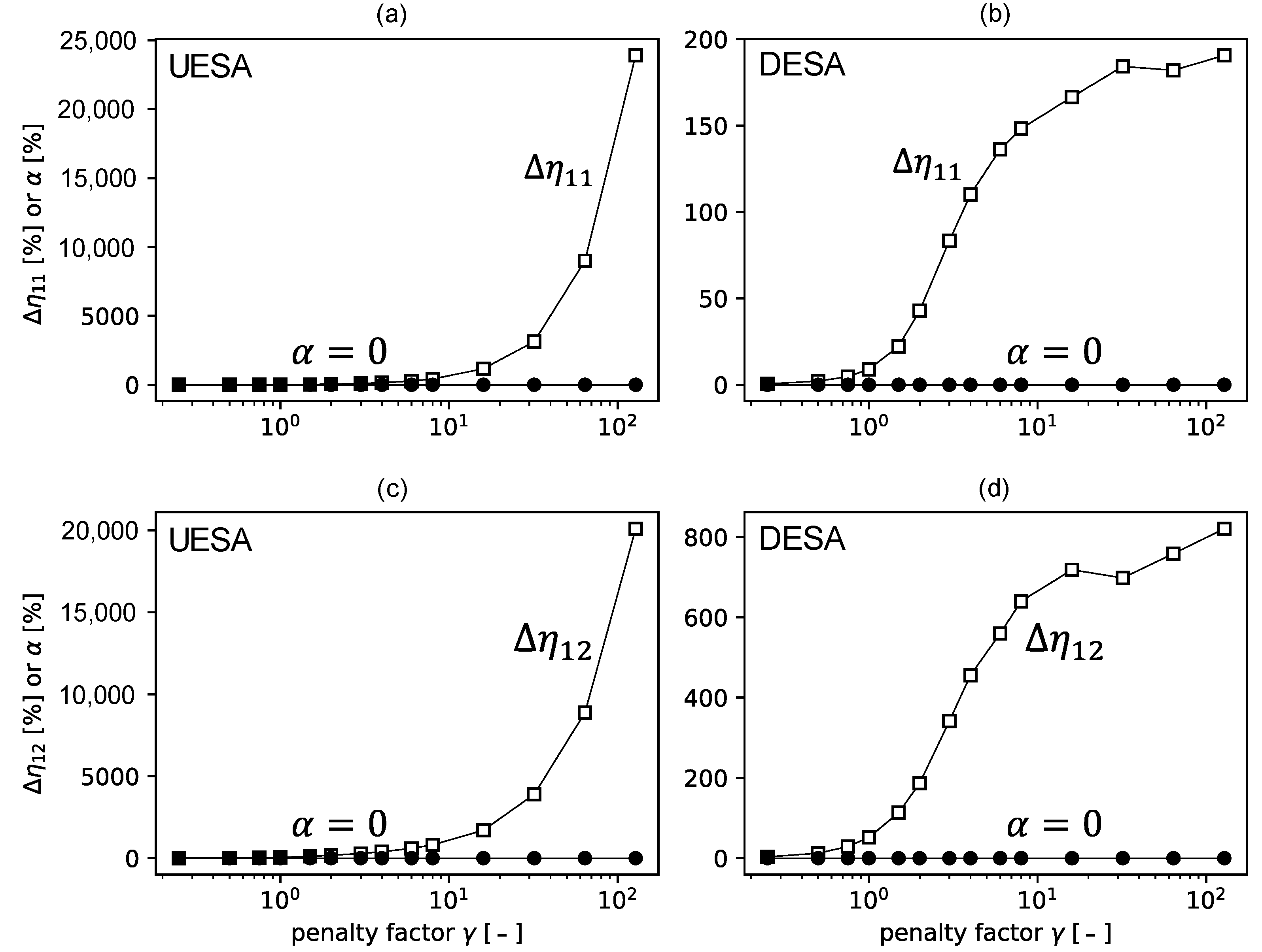
• The present paper proposes a modification of the MCF method. The modification is called DESA (Diagonal Expansion of the Search Area), which is the main contribution to the experimental SEA field. DESA consists of applying a correction during the MCF, which causes a non-uniform expansion of the search area (Section 2.1). This novel approach expands the range of vibroacoustic systems that can be properly identified by MCF. It can be applied in the frequency bands for which correct results could not be obtained using the MCF method in the basic version (using a homogeneous expansion of the search area for the population $\left\{\left[G_s\right]\right\}$ with a normal distribution), as will be demonstrated by the example presented in Section 3.
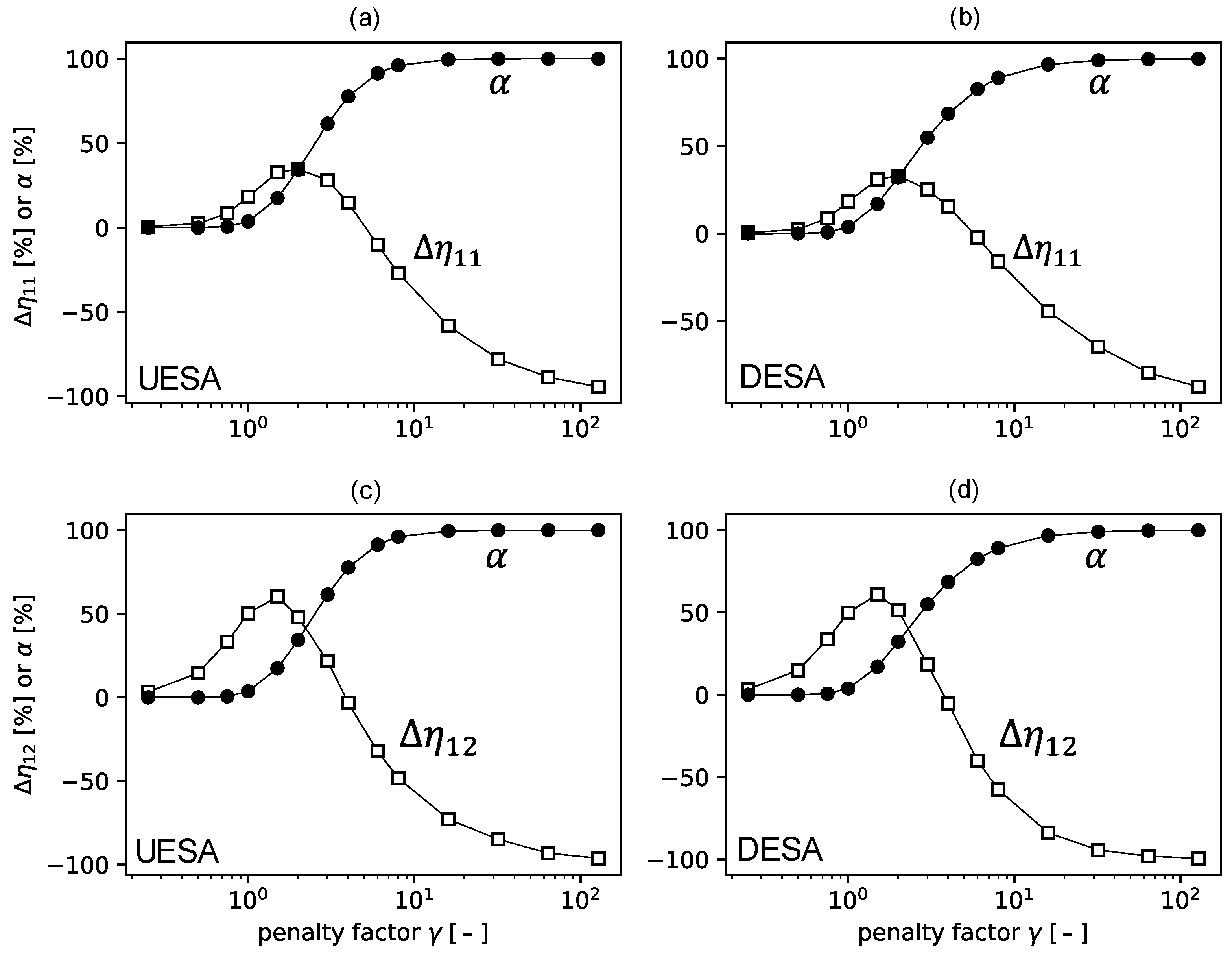
• The effect of the expansion of the search area (parameter $\gamma$) on the errors introduced into the loss factors was investigated. The so-called shift error was observed and related to the asymmetry present in the generated population of the energy matrices. We pointed out that the asymmetry of the population increases with an increase in $\gamma$.
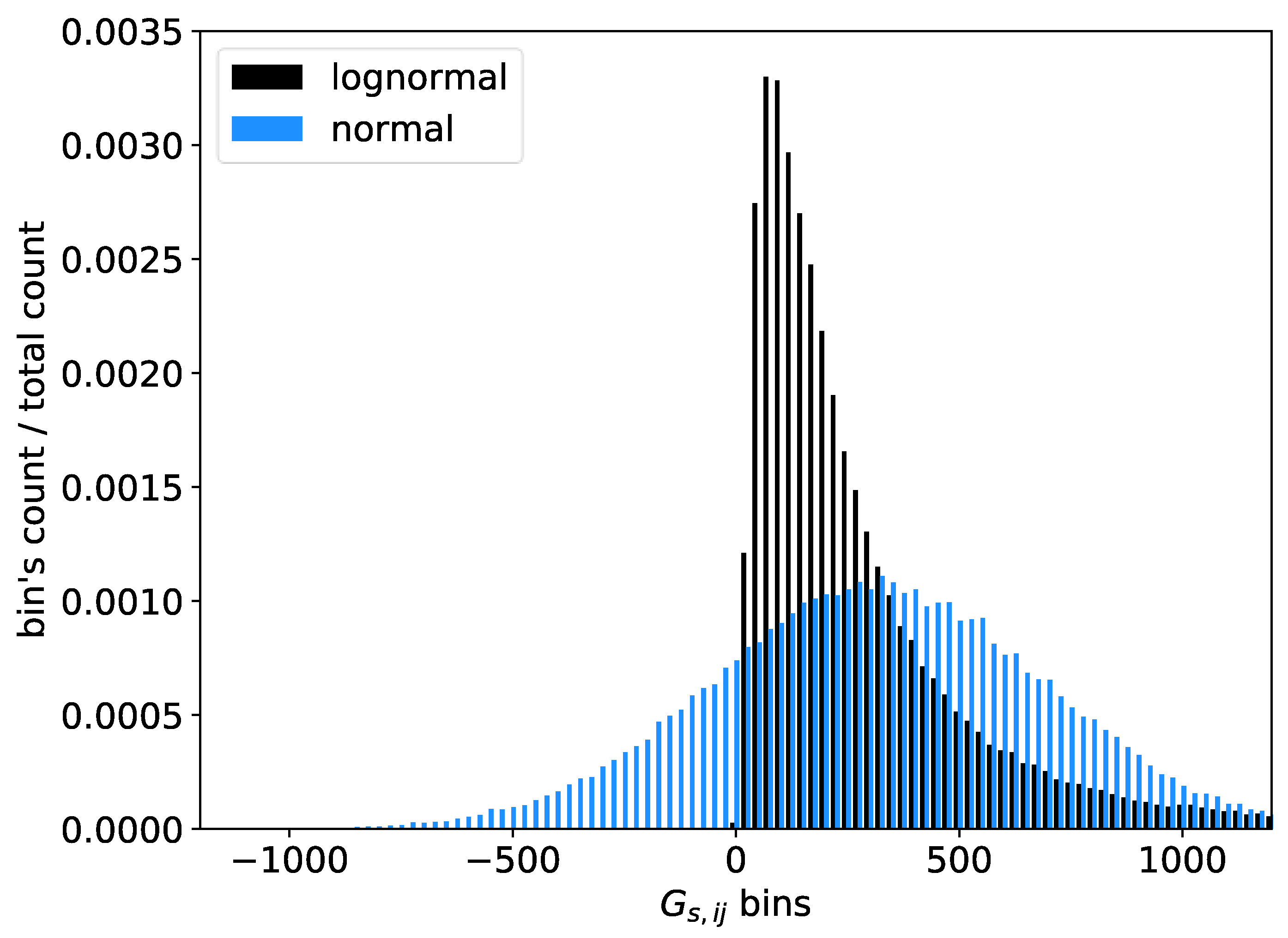
• We introduced a new parameter describing the degree of asymmetry of the energy matrix population, the asymmetry index $\alpha$, and proposed two methods (A and B) for eliminating the shift error. Method A involves detecting matrices that introduce asymmetry and rejecting them from the calculation, while method B involves using a log-normal distribution when generating the energy matrix population. A common feature of both methods is the need to perform $\gamma$ minimization.

2. Materials and Methods

This section presents the main contributions of the current paper in the E-SEA field: formulation of the DESA method (Section 2.1), and the introduction of Methods A and B, which can compensate for errors associated with ESA (Section 2.2).

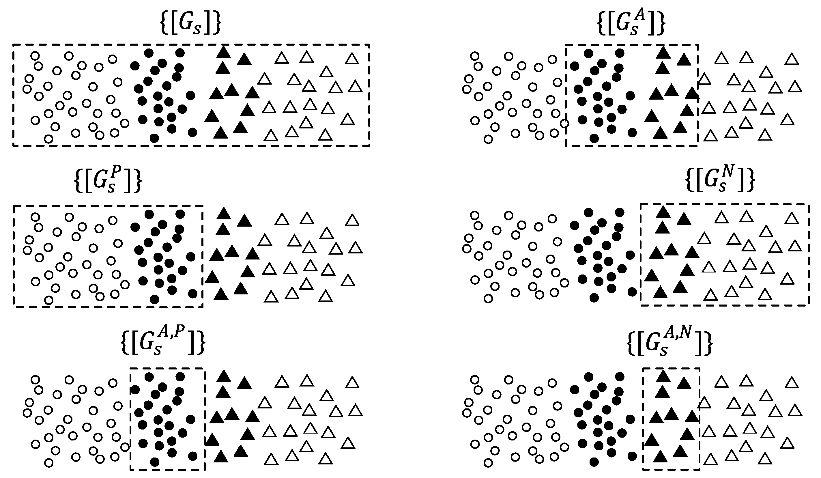
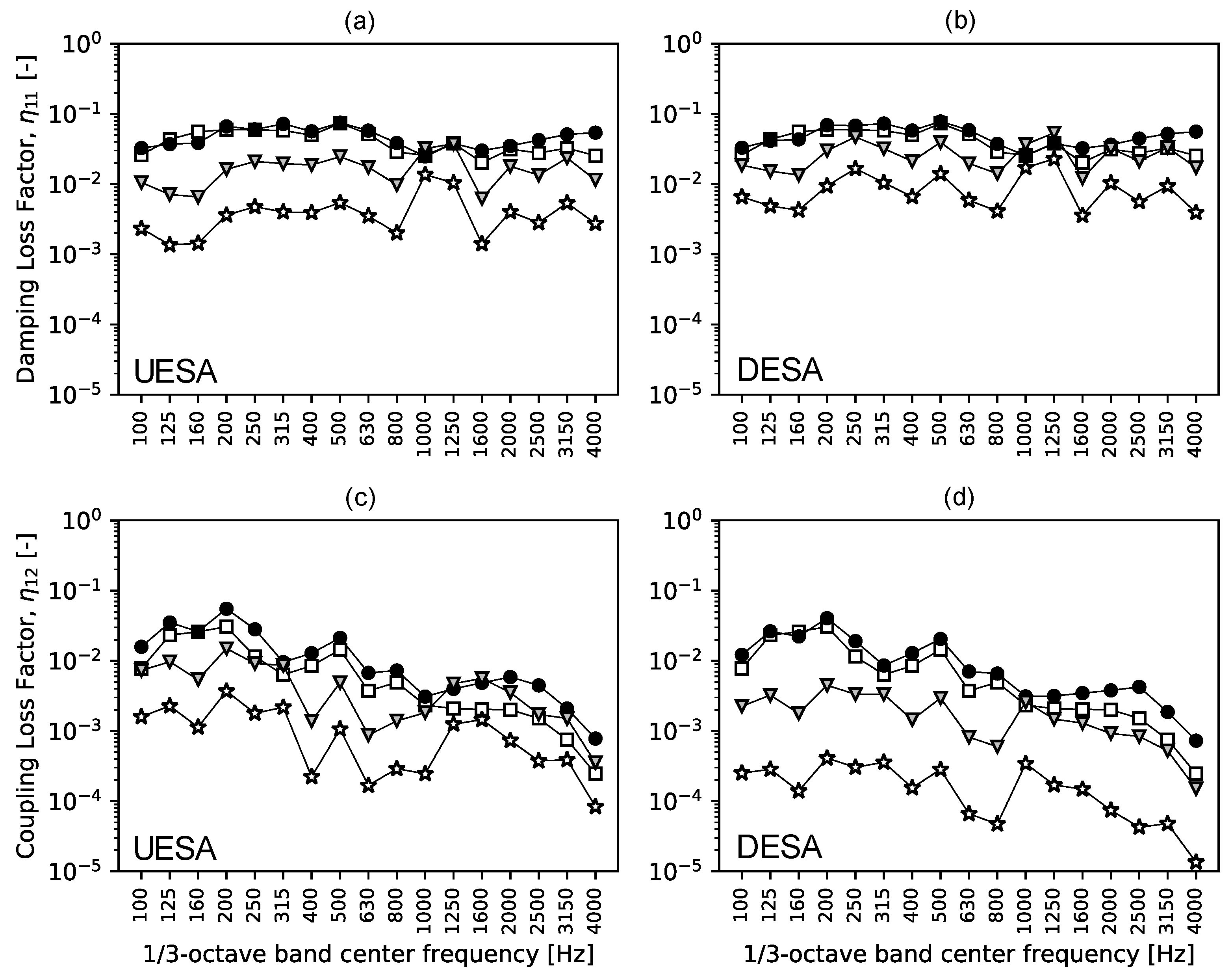
2.1. Expansion of the Search Area (UESA and DESA)

There may be cases where the standard deviations ${\sigma }_{ij}$ used in $\left[\mathsf{\Delta }G\right]$ are too small to find the correct energy matrix $\left[G_s\right]$, meaning that the set $\left\{\left[G_s^P\right]\right\}$ is empty. In order to increase the success probability of filling $\left\{\left[G_s^P\right]\right\}$, it is reasonable to use additional scaling factors ${\gamma }_{ij}>1$ gathered into the matrix $\left[\gamma \right]$. We will call the use of [γ] during the determination of the $\left[\mathsf{\Delta }G\right]$ matrix an expansion of the search area (ESA).

$$\left[\mathsf{\Delta }{G}_{ESA}\right]=\left[a\right] \circ \left[\sigma \right] \circ \left[\gamma \right]$$

(9)

However, no guidelines are given in the literature about the selection of these scaling factors, and no analysis has been formed of the effect of expanding the search area on errors in the final results.

The most intuitive way to select scaling factors seems to be to take a common scaling factor ${\gamma }_U$ for all expressions of the matrix $\left[\gamma \right]$, which in this work will be referred to as the uniform expansion of the search area (UESA). UESA can be thought of as the use of expanded measurement uncertainty, rather than standard uncertainty, when generating the population. Then, the formula for $\left[\mathsf{\Delta }{G}_{UESA}\right]$ simplifies to

$$\left[\mathsf{\Delta }{G}_{UESA}\right]=\left[a\right]\circ {\gamma }_U\left[\sigma \right]$$

(10)

Usually, after performing MCF, it is possible to obtain a non-empty set $\left\{\left[G_s^P\right]\right\}$ due to random and independent changes in the elements of the matrix. However, introducing random changes uniformly for all elements (i.e., using $\left[\mathsf{\Delta }{G}_{UESA}\right]$ increments) may not be sufficient when the elements off the main diagonal are too large. In this paper, a non-uniform expansion of the search area is proposed, namely, the introduction of a scaling factor for just the elements that are located on the main diagonal of the matrix $\left[\mathsf{\Delta }G\right]$. The method is called DESA (Diagonal Expansion of the Search Area) and takes its name from this operation. Let us assign the scaling factor acting on the main diagonal symbol ${\gamma }_D$ and call it DPF (Diagonal Penalty Factor). The matrix of energy increments then takes the form

$$\left[\mathsf{\Delta }{G}_{DESA}\right]=\left[a\right] \circ \left[\sigma \right] \circ \left[{\gamma }_D\right]$$

(11)

where the elements of the matrix $\left[{\gamma }_D\right]$ are defined as follows

$${\gamma }_D^{i,j}=\left\{\begin{array}{c} 1,\hspace{1em}\hspace{1em}if i\ne j\\ {\gamma }_D,\hspace{1em}\hspace{1em}if i=j\end{array}\right.$$

(12)

In Section 3, an example of the system for which the problem described above occurred for several frequency bands is presented. The identification of this system appeared to be impossible using MCF and MCF combined with UESA (regardless of the scaling factor adopted) for a normal population distribution. The introduction of DESA made it possible to obtain a non-empty set $\left\{\left[G_s^P\right]\right\}$ and to correct the negative LF coefficients.

2.2. Errors Associated with ESA

2.2.1. Population Asymmetry and Shift Error

In this subsection, $\left[\mathsf{\Delta }G\right],$ where it will not lead to ambiguity, will refer simultaneously to $\left[\mathsf{\Delta }G\right]$, $\left[\mathsf{\Delta }{G}_{UESA}\right]$, and $\left[\mathsf{\Delta }{G}_{DESA}\right]$.

Since the matrices $\left[G\right]$ and $\left[G\right]+\left[\mathsf{\Delta }G\right]$ are different from each other, one should also expect differences between their inverses. This leads to the conclusion that the result of an MCF simulation is always subject to some error. A different set of LF coefficients is associated with each $\left[L_s^P\right]$ matrix. The average value of the LF coefficients determined from the set $\left\{\left[L_s^P\right]\right\}$ is considered a good approximation of the true quantities. In this article, we will relate this assumption to the preservation of symmetry in the generated population of the energy matrix.

The $\left[\mathsf{\Delta }G\right]$ increments can take both positive and negative values, since they are defined with random variables $\left[a\right]$, which randomly determine their signs. When the values of the $\left[\mathsf{\Delta }G\right]$ elements are small compared to the $\left[G\right]$ elements, there is a symmetric population of matrices. In such a symmetric population, there are, with equal probability, matrices $\left[G_s\right]$ with smaller element values than the corresponding elements in $\left[G\right],$ and also matrices $\left[G_s\right]$ with larger values than in $\left[G\right]$. This results in the determination of slightly smaller, as well as slightly larger, LF coefficients, with the average value from the population being close to the CLF coefficients determined directly from $\left[G\right]$.

Note that the energy matrix $\left[G_s\right]$ cannot contain negative elements since they have no physical interpretation and always lead to incorrect loss matrices. An isolated example of a matrix with negative elements that can be wrongly classified as correct is a diagonally dominant matrix with all negative elements, for example

$$\left[G_s\right]=\left(\begin{array}{cc}-3& -20\\ -20& -3\end{array}\right)$$

To guard against drawing such samples, it is recommended to discard all matrices $\left[G_s\right]$ that have at least one negative element.

A consequence of the fact that all drawn matrices $\left[G_s\right]$ with negative elements are invalid is the possibility of producing an asymmetric population when the value of any element $\mathsf{\Delta }{G}_{ij}$ is not in the interval $\left(-G_{ij};G_{ij }\right)$. This situation can occur if there is a considerable measurement uncertainty or if an excessive scaling factor is adopted. If $\mathsf{\Delta }{G}_{ij}>G_{ij}$, the matrix $\left[G\right]+\left[\mathsf{\Delta }G\right]$ can be both correct and incorrect, but the possible “balancing” matrix $\left[G\right]-\left[\mathsf{\Delta }G\right]$ that could be drawn in subsequent iterations will always be an incorrect matrix due to the negative energy value that occurs in it. Similarly, if $\mathsf{\Delta }{G}_{ij}<-G_{ij}$, the $\left[G\right]-\left[\mathsf{\Delta }G\right]$ matrix can be both correct and incorrect, but $\left[G\right]+\left[\mathsf{\Delta }G\right]$ will always be incorrect.

The described process leads to a population that is dominated by $\left[G_s\right]$ matrices with elements larger than the original $\left[G\right]$ matrix. This imbalance after matrix inversion results in the underestimation of LF coefficients. Let us call this effect a shift error, which is an error that occurs due to operating on an asymmetric population of the energy matrices. Based on the above description, we propose the following definition of matrices that introduce asymmetry $\left[G_s^A\right]$.

Definition 1.

If the test matrix$\left[G_{s,test}\right]$corresponding to the generated matrix$\left[G_s\right]$contains at least one negative element, then$\left[G_s\right]$is a$\left[G_s^A\right]$matrix. For each$\left[G_s\right]= \left[G\right]+\left[\mathsf{\Delta }G\right]$, the test matrix can be determined from the relation$\left[G_{s,test}\right]=\left[G\right]-\left[\mathsf{\Delta }G\right]$.

Let us note that the moment of classifying a given matrix as $\left[G_s^A\right]$ occurs before its inversion, and therefore both the $\left[G_s^P\right]$ and $\left[G_s^N\right]$ matrices can be considered to be symmetry-disruptive. For the purpose of further consideration, let us mark this fact by writing the set $\left\{\left[G_s^A\right]\right\}$ as

$$\left\{\left[G_s^A\right]\right\}=\left\{\left[G_s^{A,N}\right]\right\}\cup \left\{[G_s^{A,P}]\right\}$$

(13)

The distinguished disjoint subsets of the set $\left\{\left[G_s^A\right]\right\}$ have the following interpretation. The subset $\left\{\left[G_s^{A,N}\right]\right\}=\left\{\left[G_s^A\right]\right\}\backslash \left\{[G_s^P]\right\}$ is the set of incorrect matrices that introduce asymmetry, while the complement $\left\{\left[G_s^{A,P}\right]\right\}=\left\{\left[G_s^A\right]\right\}\backslash \left\{[G_s^N]\right\}$ is the set of correct matrices that introduce asymmetry. The relations between the described sets are shown in Figure 1.

The shift error increases as the cardinality of the set $\left\{\left[G_s^{A,P}\right]\right\}$ increases relative to the cardinality of $\left\{\left[G_s^P\right]\right\}$. Let us introduce the naturally resulting definition of the population asymmetry measure from this relationship as

$$\alpha =\frac{\mathrm{card}\left(\left\{\left[G_s^{A,P}\right]\right\}\right)}{\mathrm{card}\left(\left\{[G_s^P]\right\}\right)}$$

(14)

where card (…) denotes the cardinality of the set. The asymmetry index $\alpha$ can be directly controlled by changing the values of $\left[\mathsf{\Delta }{G}_{ESA}\right]$. In turn, $\left[\mathsf{\Delta }{G}_{ESA}\right]$, according to Equation (9), depends on the scaling factor $\gamma$. Figure 2 shows the effect of changing $\gamma$ in UESA and DESA on shift errors when identifying an example system. Figure 2 was formed by sequentially recalculating Equations (10) and (11) with different values of $\left[{\gamma }_U\right]$ and $[{\gamma }_D]$ to obtain energy increments $\left[\mathsf{\Delta }{G}_s\right]$ associated with different values of $\gamma$ (2.5, 20 and 100). Then, from Equation (6) the sample energy matrix $\left[G_s\right]$ was obtained for each $\gamma$. This process was repeated 1 × 10⁵ times to obtain the populations $\left\{\left[G_s\right]\right\}$. Each energy matrix was then inverted using Equation (5) to obtain the resulting $\left\{\left[L_s\right]\right\}$ population. Next, the MCF procedure was performed, as described in “Introduction”, to obtain the set of correct matrices $\left\{\left[L_s^P\right]\right\}$. Elements of $\left\{\left[L_s^P\right]\right\}$ were averaged arithmetically to obtain $\left[L_{mean}\right]$. Then, based on Equation (2), the mean loss factors shown in the figure were extracted from $\left[L_{mean}\right]$ as follows. Coupling loss factor ${\eta }_{ij}$ is off-diagonal term $L_{ji}$ multiplied by −1, and damping loss factor ${\eta }_{ii}$ is obtained by summing the elements of column $i$.

From Figure 2, it can be seen that an increase in $\gamma$ is associated with an increase in the shift error. It can also be seen that the shift error (i.e., underestimation of LF) is most significant for large scaling factors. When the scaling factors are smaller, LF can also be observed to be larger in relation to the original values. To trace this relationship more closely, let us focus on one of the frequency bands, e.g., 800 Hz. Figure 3 shows how the relative error in determining the loss factors $\mathsf{\Delta }\eta$ (both CLF and DLF) and the population asymmetry index α change as a function of $\gamma$. For $\alpha >50\%$, the effects associated with population asymmetry begin to dominate, and an increasing shift error is observed ($\mathsf{\Delta }\eta <0$). For $\alpha <50\%$, $\mathsf{\Delta }\eta$ is positive. It is worth noting that due to $\mathsf{\Delta }\eta$ reaching a maximum for a certain ${\gamma }_{max}$, there is such a ${\gamma }_{opt }>{\gamma }_{max}$ for which $\mathsf{\Delta }\eta =0$.

2.2.2. Scaling Factor Minimization

It follows from the considerations in Section 2.2.1 that small values of $\gamma$ lead to a minimization of the shift error. A zero $\mathsf{\Delta }\eta$ error can also be achieved by using the ${\gamma }_{opt}$ value for ESA (${\gamma }_{opt}>{\gamma }_{max}>0$), but finding ${\gamma }_{opt}$ in practice is problematic or even impossible (a small error in the estimation of ${\gamma }_{opt}$ results in a large change in $\mathsf{\Delta }\eta$). A more practical solution seems to be to perform $\gamma$ minimization.

To minimize $\gamma$, one can use an algorithm of choice, such as a simple search, the principles of which are reflected in Figure 4. As can be seen, a starting value of ${\gamma }_0=1$ proved to be insufficient to determine the correct loss matrix. In step No. 1, the value of ${\gamma }_1=2{\gamma }_0$ also had no effect. The correct matrix was obtained in iteration No. 2 for ${\gamma }_2=2{\gamma }_1$. In step No. 3, one went back to the value of ${\gamma }_3=\left({\gamma }_1+{\gamma }_2\right)/2,$ and again the wrong matrix was determined. In step No. 4, the value of $\gamma$ was increased to ${\gamma }_4=\left({\gamma }_3+{\gamma }_2\right)/2$, and as a result, the correct matrix was obtained and the stop condition was satisfied (the sought optimum value of ${\gamma }_5$ was approached).

The optimization process is stochastic (each matrix contains a random element in it), and therefore each execution of the process may indicate a slightly different optimal value. The solution to the problem may be to run the optimization multiple times, and then to determine the average value or to choose the minimum value from all the processes. The presented example illustrates that the proposed method can be time-consuming and should therefore only be used for problematic frequency bands.

2.2.3. Enforcing Symmetry of the Population

Performing $\gamma$ minimization (Section 2.2.2) is necessary to generate correct matrices lying in the closest vicinity of the original matrix. The minimization of $\gamma$, however, does not completely eliminate the shift error, but only minimizes it (the matrices inducing the shift error may still be present in the set $\left\{\left[G_s^P\right]\right\}$). In this section, we propose two methods to eliminate the shift error, which involve forcing the symmetry of the population of energy matrices (SFM, Symmetry Forcing Methods):

• Method A, which involves discarding from the calculation matrices that fall into the tail of the normal distribution.
• Method B, which involves generating a population with a log-normal distribution.
• The use of one of the presented SFM methods in combination with $\gamma$-minimization allows us to:
  • Correct negative loss factors and replace them with factors that are free of offset error.
  • Obtain results close to the original results in bands that do not require correction, which can be good in terms of the quality control of the applied methods.

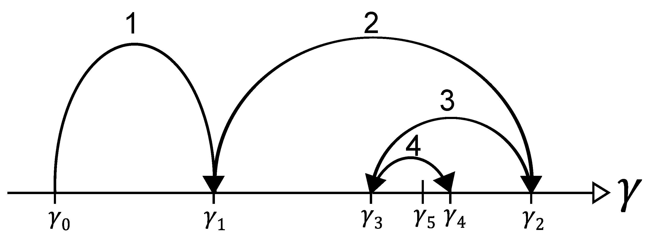
Method A makes it possible to enforce the symmetry of the population by excluding the set $\left\{\left[G_s^A\right]\right\}$ from the calculation, where $\left\{\left[G_s^A\right]\right\}$ can be detected based on the definitions presented in Section 2.2.1. Let us follow this process for a selected frequency (3150 Hz) and an element (I = 1, j = 2) of the $\left\{\left[G_s\right]\right\}$ from Section 3. Figure 5 shows the histogram of the analyzed element (1 × 10⁵ samples). As expected, the population generated from Formulas (6) and (8) has a normal distribution. Method A is based on the rejection of elements introducing asymmetry, as seen in Figure 5.

It can be seen from the figure that it is necessary to detect the correct value between 0 and $2G_{ ij}$, where $G_{ ij}$ is an element from the original measurement matrix $\left[G\right]$. The fulfillment of this condition in the context of the matrix population depends on the relationship between the cardinality of the set $\left\{\left[G_s^P\right]\right\}$ and $\left\{\left[G_s^{A,P}\right]\right\}$. There are two possible identification results with A:

• When $\mathrm{card}\left(\left\{\left[G_s^P\right]\right\}\right)>\mathrm{card}\left(\left\{\left[G_s^{A,P}\right]\right\}\right)$, or equivalently $\alpha <1$, the result obtained will be free of both shift error and negative LF. Then, the identification result obtained by Method A can be considered correct, and $\alpha = 0$ occurs for the resulting population.
• When $\mathrm{card}\left(\left\{\left[G_s^P\right]\right\}\right)= \mathrm{card}\left(\left\{\left[G_s^{A,P}\right]\right\}\right)$, or equivalently $\alpha = 1$ (which also means that $\left\{\left[G_s^P\right]\right\}=\left\{\left[G_s^{A,P}\right]\right\}$), all correct matrices will be discarded and the correction of negative LF coefficients will not take place. Method A is then ineffective. However, it is possible to take the LF coefficients determined for an asymmetric population of matrices as the final result. In such a situation, the result obtained will be affected by a shift error. However, this error will be minimized by using ${\gamma }_{min}$ during the calculation (the distance between the matrices $\left[G_s^A\right]$ and the original matrix $\left[G\right]$ will be relatively small).

Figure 6 shows how $\Delta \eta$ and $\alpha$ change as a function of $\gamma$ when Method A is applied. Of course, due to the rejection of all samples from $\left\{\left[G_s^{A,P}\right]\right\}$, we have $\mathrm{card}\left(\left\{\left[G_s^{A,P}\right]\right\}\right)=0\to \alpha =0$. Note that Method A eliminates from the population only those matrices that introduce error due to asymmetry. Forcing symmetry cannot cancel the errors caused by the presence of matrices $\left[G_s^P\right]$ in the population that are significantly distant from the original $\left[G\right]$ (large values of $\mathsf{\Delta }\eta$ for large $\gamma$ in Figure 6). When a given population is formed on the basis of a huge scaling factor, Method A will provide the result associated with the broadest possible increase in $\mathsf{\Delta }G$, which does not introduce asymmetry (the area of stabilization of $\mathsf{\Delta }\eta$ in Figure 6, well seen especially in Figure 6b,d) Figure 6a,c also shows the case when the population before symmetry forcing was characterized by $\alpha = 1$ for a sufficiently large $\gamma$. Then, all $\left[G_s^P\right]$ were in the discarded region, and determining the loss factors was impossible.

For the reasons mentioned above, it is strongly discouraged to take arbitrarily large values of $\gamma$ during ESA operations and to omit the minimization of $\gamma$ based on the erroneous assumption that Method A can correct the result automatically. For example, Figure 7a,c shows the effect of Method A on an asymmetric population generated with $\gamma =100$ (DESA). It can be seen that the shift error (underestimation of the result) has been removed, but the final result is overestimated. Figure 7b,d, on the other hand, concerns the asymmetric population generated with $\gamma =1.5$. In this case, the search area was narrower, and more matrices closer to the original one were included in the population. For this reason, the LF coefficients in Figure 7b,d are closer to the result of the experiment without using MCF. Therefore, the problem described above should be of little importance when the γ-minimization procedure is carried out before proceeding with SFM.

Since the case $\alpha =1$ may occur, where Method A is unreliable, we propose an alternative approach that enforces population symmetry—Method B. So far, our considerations have been carried out assuming a normal distribution of the population of generated energy matrices based on Equation (6). Note that by changing this approach and assuming a log-normal distribution, we naturally exclude all matrix elements with negative values from the procedure (Figure 8). In turn, the dominants of the individual elements are smaller than the corresponding values of the elements in $\left[G\right]$. For a population with a log-normal distribution, asymmetry does not arise ($\alpha =0$ always occurs, and shift error does not occur).

The parameters $\mu$ and ${\sigma }^2$ of the log-normal distribution can be determined from the relationship [26].

$$\mu =ln\left(\frac{{\mu }_X^2}{\sqrt{{\mu }_X^2+{\sigma }_x^2}}\right)$$

(15)

$${\sigma }^2=ln\left(1+\frac{{\sigma }_x^2}{{\mu }_X^2}\right)$$

(16)

which allows the obtaining of the mean ${\mu }_X$ and the variance ${\sigma }_x^2$ of the log-normal distribution to be equal to that of the normal distribution from Method A.

Figure 9 shows an example of the dependence of $\alpha$ and $\mathsf{\Delta }\eta$ on $\gamma$ when a log-normal distribution is assumed. As in Method A, the error in determining the loss factor $\mathsf{\Delta }\eta$ increases with an increasing $\gamma$. However, the error in $\mathsf{\Delta }\eta$ does not stabilize for some sufficiently large $\gamma$, but increases unlimitedly. Particularly large values can be seen in Figure 9a,c. This is because in Method B, there is no need to exclude from the calculation values the falling into the tail of the distribution. The error $\mathsf{\Delta }\eta$ converges to zero for a small $\gamma$, as in Method A. Thus, the minimization of $\gamma$ is also necessary in Method B.

3. Results

Power injection method (PIM) measurements were carried out using MCF on a structure composed of two steel beams connected to each other at right angles. The mechanical and geometric parameters of the subsystems are given in

Table 1. Mechanical and geometric parameters of the subsystems.

Geometry
Thickness	20 mm
Length	80 mm
Width	500 mm
Mechanical Parameters
Material	Steel
Density	7827 kg/m3
Young’s modulus	205 GPa
Poisson number	0.3

.

Both flexural and longitudinal waves were considered in the SEA model. This resulted in the system being divided into four subsystems: the flexural wave field of beam 1, the longitudinal wave field of beam 1, the flexural wave field of beam 2, and the longitudinal wave field of beam 2. The loss matrix and energy matrix were therefore 4 × 4 in size.

Figure 10 shows the values of the CLF (${\eta }_{12}$) that describe the energy flow between the flexural wave field of beams 1 and 2 as a function of frequency. In turn, Figure 11 shows the values of two selected elements of the energy matrix for all the Monte Carlo iterations carried out for the selected frequency of 250 Hz. The elements $G_{s,22}$ were on the main diagonal, while the elements $G_{s,23 }$ were off the main diagonal. The red dots on the graphs indicate the iterations where the correct matrices $\left[G_s^P\right]$ were detected.

4. Discussion

Figure 10 shows that the application of the MCF method in its basic version (i.e., without expanding the search area in a population with a normal distribution) failed to determine positive loss factors in the 1/3-octave bands of 250 Hz, 315 Hz, and 3150 Hz. For 250 Hz, this situation corresponds to Figure 11a. The energy matrix has no possibility of becoming a diagonally dominant matrix (the energy of a subsystem is higher when it is a source subsystem, and lower when it is a receiving subsystem) due to the fact that $G_{s,22}<G_{s,23}$ occurs in almost every iteration. However, there is a non-zero probability of $G_{s,22}>G_{s,23}$ occurring. Based on the tracking of a single pair of elements, one cannot draw any conclusion about the entire energy matrix. The condition $G_{s,22}>G_{s,23}$ is, of course, necessary, but is not sufficient for the matrix $\left[G_s\right]$ to be a diagonally dominant matrix. A sufficient condition is the fulfillment of the set of conditions $G_{s,jj}>G_{s,ji},i\ne j$ for each row $j$. In the case of the 4 × 4 matrix in question, the probability of simultaneously satisfying each condition turned out to be unacceptably small. The number of iterations in Figure 11a is equal to 1 × 10⁵, but trials continued (unsuccessfully) until the number of iterations reached 2 × 10⁷.

Figure 11b shows that the use of UESA with $\gamma =20$ only resulted in an even shift in the values of the two elements of the matrix and did not improve the efficiency of the applied method.

The calculations in Figure 11c used DESA with a minimized DPF value of $\gamma =6$, resulting in a non-empty set $\left\{\left[G_s^P\right]\right\}$. Figure 10 shows that the CLF spectrum obtained in this way is subject to shift error. For the case under consideration, $\alpha =1$ also occurred. Indeed, after forcing the symmetry of the population using Method A (Figure 11d), the set $\left\{\left[G_s^P\right]\right\}$ again became empty since all the correct matrices were in the tail of the normal distribution.

Using a log-normal distribution of the population according to Method B (Figure 11e for DESA and 11f for UESA) proved to be effective. Positive loss factors with no shift error were obtained, as can be seen in Figure 10. It was noted that by using $\gamma$ minimization for a log-normal distribution, much smaller optimal values of $\gamma$ can be obtained when compared to a population with a normal distribution (in the case in question, $\gamma =1.5$). This made it possible to obtain loss factor values close to the original values in the uncorrected bands.

The above analysis clearly shows the advantage of the proposed method compared to the previously known approaches. The standard method (MCF procedure with UESA) was insufficient to correct negative loss factors in the considered case because energy terms could not match requirements in any Monte Carlo iteration. On the other hand, the proposed method DESA and standard UESA combined with new error correction methods A and B were successful. In other words, the proposed approach’s novelty results from extending the range of potential vibroacoustic systems that can be properly identified in E-SEA (with minimized error and without negative loss factors). Therefore, this case study confirms the paper’s main contributions indicated in the Section 1.

5. Conclusions

The paper proposes a modification of the MCF method. The modification is called DESA and involves the use of a non-uniform expansion of the search area (using scaling factor $\gamma$, DPF) during Monte Carlo population generation and also makes it possible to correct negative loss factors in frequency bands that are problematic for the MCF method.

The paper analyzed the effect of the degree of search area expansion on the resulting errors introduced into the loss factors. A so-called shift error was observed, which was related to the asymmetry present in the generated population of the energy matrix. It was pointed out that the asymmetry of the population increases with the expansion of the search area and is due to the domination of the population by matrices with elements larger than in the original experimentally determined matrix. The favoritism of matrices with large elements is related to the presence in the population of always incorrect and rejected matrices containing negative elements, which occurs when the values of the applied energy increments are larger than the values of the elements of the original matrix. A new parameter α was proposed to describe the degree of asymmetry of the population of energy matrices, as well as two methods for compensating for the shift error: Method A and Method B.

Method A involves performing DPF minimization and rejecting matrices that introduce asymmetry from the calculation. Method A is applicable when α < 1, and therefore is not including the possible case of α = 1.

Method B proposes an alternative model for matrix population generation using a log-normal distribution and by performing DPF minimization. Method B is free of the limitations of Method A and allows for the correction of negative loss factors with the use of smaller DPF values when compared to Method A, which is based on a normal distribution of matrix elements.

The DESA method was tested on a system consisting of two steel beams, where the SEA model took into account the phenomenon of wave conversion (four subsystems). During the determination of the loss factors of the tested system, the proposed methods for minimizing the shift error were also applied, and the superiority of Method B was demonstrated. Replacing UESA with the DESA method allowed for the correction of the negative loss factors, but Method A did not enable the shift error to be removed. The best results were obtained by using Method B, which made it possible to cancel the shift error and use smaller optimal scaling coefficients.

References

1. Lyon, R.H.; DeJong, R.G.; Heckl, M. Theory and Application of Statistical Energy Analysis. J. Acoust. Soc. Am. 1995, 98, 3021. [Google Scholar] [CrossRef]
2. Hwang, H.J. Prediction and Validation of High Frequency Vibration Responses of NASA Mars Pathfinder Spacecraft due to Acoustic Launch Load Using Statistical Energy Analysis. Technical report, California Institute of Technology, Jet Propulsion Laboratory. 28 April 2002. Available online: https://trs.jpl.nasa.gov/bitstream/handle/2014/11593/02-0107.pdf?sequence=1 (accessed on 12 December 2022).
3. Chen, X.; Wang, D.; Ma, Z. Simulation on a car interior aerodynamic noise control based on statistical energy analysis. Chin. J. Mech. Eng. 2012, 25, 1016–1021. [Google Scholar] [CrossRef]
4. Craik, R. The prediction of sound transmission through buildings using statistical energy analysis. J. Sound Vib. 1982, 82, 505–516. [Google Scholar] [CrossRef]
5. Bies, D.; Hamid, S. In situ determination of loss and coupling loss factors by the power injection method. J. Sound Vib. 1980, 70, 187–204. [Google Scholar] [CrossRef]
6. Iwaniec, M. Damping loss factor estimation in plates. Mol. Quantum Acoust. 2003, 24, 61–68. [Google Scholar]
7. Bloss, B.; Rao, M.D. A Comparison Between Power Injection and Impulse Response Decay Methods for Estimating Frequency Averaged Loss Factors for SEA. SAE Trans. 2003, 1878–1890. [Google Scholar] [CrossRef]
8. Fahy, F.J.; Ruivo, H.M. Determination of statistical energy analysis loss factors by means of an input power modulation technique. J. Sound Vib. 1997, 203, 763–779. [Google Scholar] [CrossRef]
9. Sun, J. Measuring Method of Dissipation and Coupling Loss Factors for Complex Structures. In Chinese Science Abstracts Series A; Elsevier Science: Amsterdam, The Netherlands, 1995; Volume 4, Number 14; p. 24. [Google Scholar]
10. Gu, J.; Sheng, M. Improved energy ratio method to estimate coupling loss factors for series coupled structure. J. Mech. Eng. 2015, 45, 37–40. [Google Scholar] [CrossRef] [Green Version]
11. Cuschieri, J.; Sun, J. Use of Statistical Energy Analysis for Rotating Machinery, Part I: Determination of Dissipation and Coupling Loss Factors Using Energy Ratios. J. Sound Vib. 1994, 170, 181–190. [Google Scholar] [CrossRef]
12. Guasch, O. A direct transmissibility formulation for experimental statistical energy analysis with no input power measurements. J. Sound Vib. 2011, 330, 6223–6236. [Google Scholar] [CrossRef]
13. Fahy, F. An alternative to the SEA coupling loss factor: Rationale and method for experimental determination. J. Sound Vib. 1998, 214, 261–267. [Google Scholar] [CrossRef]
14. Ming, R. An experimental comparison of the sea power injection method and the power coefficient method. J. Sound Vib. 2005, 282, 1009–1023. [Google Scholar] [CrossRef]
15. Ming, R. The measurement of coupling loss factors using the structural intensity technique. J. Acoust. Soc. Am. 1998, 103, 401–407. [Google Scholar] [CrossRef]
16. Cacciolati, C.; Guyader, J.L. Measurement of SEA coupling loss factors using point mobilities. Philosophical Trans-actions of the Royal Society of London. Ser. A Phys. Eng. Sci. 1994, 346, 465–475. [Google Scholar]
17. Hopkins, C. Statistical energy analysis of coupled plate systems with low modal density and low modal overlap. J. Sound Vib. 2002, 251, 193–214. [Google Scholar] [CrossRef]
18. Lalor, N. Practical Consideration for the Measurement of Internal and Coupling Loss Factors on Complex Structures, ISVR Technical Report No. 182. June 1990.
19. de las Heras, M.F.; Manguán, M.C.; Millán, E.R.; de las Heras, L.F.; Hidalgo, F.S. Determination of SEA loss factors by Monte Carlo Filtering. J. Sound Vib. 2020, 479, 115348. [Google Scholar] [CrossRef]
20. Liesen, J.; Rozlozník, M.; Strakos, Z. Least squares residuals and minimal residual methods. SIAM J. Sci. Comput. 2002, 23, 1503–1525. [Google Scholar] [CrossRef] [Green Version]
21. Hodges, C.; Nash, P.; Woodhouse, J. Measurement of coupling loss factors by matrix fitting: An investigation of numerical procedures. Appl. Acoust. 1987, 22, 47–69. [Google Scholar] [CrossRef]
22. Lawson, C.L.; Hanson, R.J. Solving Least Squares Problems; Society for Industrial and Applied Mathematics: Philadelphia, PA, USA, 1995. [Google Scholar]
23. Cimerman, B.; Bharj, T.; Borello, G. Overview of the Experimental Approach to Statistical Energy Analysis. In SAE Conference Proceedings P; Soc Automative Engineers Inc.: Warrendale, PA, USA, 1997; Volume 2, pp. 783–788. [Google Scholar]
24. Bouhaj, M.; von Estorff, O.; Peiffer, A. An approach for the assessment of the statistical aspects of the SEA coupling loss factors and the vibrational energy transmission in complex aircraft structures: Experimental investigation and methods benchmark. J. Sound Vib. 2017, 403, 152–172. [Google Scholar] [CrossRef]
25. Horn, R.A.; Johnson, C.R. Matrix Analysis; Cambridge University Press: Cambridge, UK, 2012. [Google Scholar]
26. Jobe, J.M. Log-Normal Distributions: Theory and Applications; Dekker: New York, NY, USA, 1989. [Google Scholar]
Figure 1. Subsets of the set G s . ○: matrices that are correct and do not disturb symmetry, ●: correct matrices that disturb symmetry, ▲: incorrect matrices that disturb symmetry, △: incorrect matrices that do not disturb symmetry.
Acoustics 04 00063 g001
Figure 2. Effect of the scaling factor on shift errors. □—without MCF, ●: γ = 2.5 , : γ = 20 , ☆: γ = 100 . (a) UESA, DLF; (b) DESA, DLF; (c) UESA, CLF; (d) DESA, CLF. UESA: uniform expansion of the search area, DESA: diagonal expansion of the search area, DLF: damping loss factor, CLF: coupling loss factor.
Acoustics 04 00063 g002
Figure 3. The dependence of the error of loss factors (□) and the population asymmetry index (●) as a function of the scaling factor for a matrix population with a normal distribution. (a) UESA, DLF; (b) DESA, DLF; (c) UESA, CLF; (d) DESA, CLF.
Acoustics 04 00063 g003
Figure 4. Simple search algorithm for selecting the optimal scaling factor.
Acoustics 04 00063 g004
Figure 5. Histogram of the selected item G s , i j (i = 1, j = 2) from a population with a normal distribution.
Acoustics 04 00063 g005
Figure 6. Dependence of the error of loss factors (□) and the population asymmetry index (●) on the scaling factor for a matrix population with a tail-free normal distribution. (a) UESA, DLF; (b) DESA, DLF; (c) UESA, CLF; (d) DESA, CLF.
Acoustics 04 00063 g006
Figure 7. Loss factors after applying Method A with arbitrary scaling factor values (influence of minimization omission). □—the original value, —the value after expanding the search area, ●—the value after forcing the symmetry of the population using Method A. (a) DLF for γ = 100 , (b) DLF for γ = 1.5 , (c) CLF for γ = 100 , (d) CLF for γ = 1.5 .
Acoustics 04 00063 g007
Figure 8. Histogram of the selected item G s , i j (i = 1, j = 2) from a population with a log-normal distribution.
Acoustics 04 00063 g008
Figure 9. Dependence of the error of loss factors (□) and the population asymmetry index (●) on the scaling factor for a matrix population with log-normal distribution. (a) DLF for γ   =   100 , (b) DLF for γ   =   1.5 , (c) CLF for γ   =   100 , (d) CLF for γ   =   1.5 .
Acoustics 04 00063 g009
Figure 10. CLF coefficients between the flexural wave fields of the measured beams. —MCF without ESA; ●—MCF+DESA with minimized γ = 6; □—MCF+UESA with forced population symmetry (Method B), γ = 1.5. Red circles indicate frequency bands where MCF without ESA was not successful.
Acoustics 04 00063 g010
Figure 11. Values of elements G_ (s,22) () and G_ (s,23) (▬) for all the Monte Carlo iterations. Red dots indicate iterations with the correct loss matrix. (a) no ESA; (b) UESA with γ = 20; (c) DESA with γ = 6; (d) DESA with γ = 6 + Method A; (e) DESA with γ = 1.5 + Method B; in this variant only one correct matrix (area indicated by the red circle) was found (f) UESA with γ = 1.5 + Method B.
Acoustics 04 00063 g011