Article

Impact of Damping on Oscillation Patterns on the Plain Piano Soundboard

Institute of Systematic Musicology, University of Hamburg, Neue Rabenstr. 13, 20354 Hamburg, Germany
*
Author to whom correspondence should be addressed.
Acoustics 2022, 4(4), 1013-1027; https://doi.org/10.3390/acoustics4040062
Submission received: 11 October 2022 / Revised: 18 November 2022 / Accepted: 24 November 2022 / Published: 2 December 2022
(This article belongs to the Special Issue Vibration and Noise)

Abstract

:
The influence of internal damping on the vibration of a piano soundboard is investigated using a Finite-Difference Time Domain (FDTD) physical model and experimental measurements. The damping constant of the model is varied according to a range similar to those found with measurements on a real grand piano at different production stages. With strong damping, a clear driving-point dependency of the forced string oscillation on the oscillation pattern of the soundboard is found. When decreasing the damping, this driving-point dependency is decreasing, nevertheless, it is still present. High damping, therefore, decreases soundboard vibration when strings drive the soundboard at the soundboard’s eigenfrequencies. However, such large damping increases soundboard vibrations when strings drive the soundboard at frequencies which are not eigenfrequencies. Therefore, strong damping smooths out the frequency response spectrum of an instrument. Extreme damping without any presence of distinct eigenmodes leads to a radiation of the strings sound spectrum without soundboard filtering. Low damping leads to a strong influence of the soundboard on the string’s radiated sound. Therefore, the amount of soundboard characteristics can be designed to alter internal damping process by choice of materials, including wood or varnish, and geometry. Additionally, damping reduces the presence of ’dead spots’, notes which are considerably lower in volume compared to other notes.

1. Introduction

A vibrational system has basically two types of damping, external damping caused by energy loss due to radiation and internal damping caused by energy loss within the structure. The reasons for the internal energy loss are not yet perfectly clear [1]. There are thermodynamic losses [2] of several kinds, viscoelastic losses due to shearing, atomistic, and quantum mechanical considerations of molecular conformation [3,4], among other approaches to explain this phenomenon. When utilized in industrial applications, simple models are used to explain damping, such as the Maxwell or Voigt model, or combinations of them, as simple mass-spring systems mounted in parallel or serially [5]. Basic damping materials are bitumen, composite materials, or embedded nanotubes. Sandwich constructions, today often preferred by instrument makers, are known to have increased damping [6]. Metamaterials, e.g., periodically stiffened plates, can be designed to show a frequency band-gap damping behavior [7]. Therefore, due to the regular bracing of piano or guitar soundboards, they might behave as metamaterials and show some properties not expected from simple plates.
The complex nature of internal damping is also evident in wood. A review paper [8], reporting data of 450 wood species, finds a close correlation between Young’s modulus and the damping parameter tan δ , the relation between imaginary and real parts of a complex Young’s modulus, an index often used when measuring viscoelasticity. This index is not taking the frequency dependency of damping into consideration. Damping correlates with the Young’s modulus, however, not with wood density [9]. Comparing normal wood and compression wood (with a higher amount of cellulose), it appears that the microfiber angle (MFA), the angle the cellulose fibers lay inside the second cell wall, correlates with both Young’s modulus and damping [10].
Internal damping of wood for soundboards of musical instruments has only slightly been investigated. Obataya et al. investigate the influence of viscoelasticity on the vibration of reeds [11]. The application of varnish considerably increases the damping. Schleske [12] finds the damping increased by up to 75% depending on the kind and thickness of the varnish. Schelleng reports a considerable increase in the logarithmic decrement, from 0.4 up to 0.8, when adding varnish to a violin. Both find a slight decrease in radiation strength around 1–3 dB, which is nearly not audible, and a slight decrease in eigenfrequencies, as expected.
Another way to dampen soundboards is to adjust their boundary conditions. From the perspective of an instrument maker, a plate with a thin boundary region may be called a diaphragmatic or ’membrane-like’ plate. When measuring all available Torres guitars, Romanillos [13] found that a common feature is a decrease in the top-plate thickness towards the boundaries. He reports that the center of the guitar top plates have an average thickness of 2.5 mm, while the boundaries are only 1.4 mm thick on average. Using his famous paper mache guitar consisting of a regular top plate but having paper mache ribs and back, Torres tried to show that the sound of his guitar is solely radiated from the top plate. This guitar still has bracings and rims on the backplate to make it statically stable. Its top plate boundary thickness is decreased down to 0.4 mm. Still, this may be caused by later repairs. When knocking on Torres guitars, Romanillos finds the sound to be “short and muffled” (p. 120) and more membrane-like than as a plate.
A similar approach in piano making has been reported by Hansing [14], as well as Bilhuber [15,16], namely thinning the soundboard of pianos towards the boundaries. This approach is called a “diaphragmatic plate”, where the plate is supposed to act as a membrane rather than a plate due to its boundary conditions. The resulting sound is described by Bilhuber as bright and full and desirable for instrument makers.
However, strictly speaking, this membrane behavior can only hold for the boundary region of the plate, where it has a thickness h 2 mm. Such a small thickness cannot appear over the whole size of the plate, since then it would not be able to statically withstand the down-force resulting from the strings. Therefore, in its center section the plate will vibrate like a plate, with a bending stiffness as its cause, and only at the boundary regions show membrane-like behavior.
Another approach to understanding the idea of Torres and diaphragmatic plates is discussed within the Acoustic Black Hole (ABH) theory in search of lightweight and effective damping plates [17]. There it was found that plates with a thickness slowly decreasing to zero show no reflection at the boundaries because of a slowly decreasing wave speed, which becomes theoretically zero at the plate boundary of zero thickness. Then no waves are reflected, leading to a total dissipation.
Another point discussed is the pre-stress of piano soundboards. Piano makers can adjust the amount of down-force acting on the soundboard by changing the angle of the strings crossing the bridge, as well as through crowning, the convex bending of the soundboard [18,19]. Using the string rods to hold the strings on the bridge points, the adjustment of the string tension onto the soundboard can be modified to such an extent that nearly no tension is acting on the soundboard. Such experiments were performed towards the end of the 19th century, but were not prolonged as builders had the impression that the sound of the piano was losing brightness or ’bite’ [14,20].
To estimate the influence of internal damping on the vibration of a piano soundboard, in this study, using a physical model, the damping is varied in steps, and the soundboard is driven at different bridge positions. Additionally, two driving mechanisms are used, a sinusoidal and an impulse driving, both methods often used when investigating soundboards experimentally.
When playing piano, the vibration of the soundboard is not that of eigenvalues but of a forced oscillation, where the string forces the soundboard to vibrate in the strings frequencies. Since the string has almost no sound radiation and the sound is almost only radiated from the soundboard, this is a necessary prerequisite in order to hear the string frequencies and thus the keys played on the piano and not the natural modes of the piano soundboard.
A Finite-Difference Time Domain (FDTD) method is applied to a model of a raw piano soundboard, comparing it to measurements on a real raw soundboard with the same dimensions. The reason for taking a raw soundboard without ribs and bridges, not yet being glued to a piano frame, is that it assures the observed findings only to depend on the internal damping and not on a complex geometry. Still, measurements from a finished soundboard are included and used to find the range of internal damping for piano soundboards at different production stages. Discussing details of the extensive measurements on the soundboard is beyond the scope of this paper and is to be published in the future.

2. Methods

2.1. Finite-Difference Model

The differential equation of the plate used is
2 E ( x , y ) h ( x , y ) 3 3 ( 1 ν 2 ) ϱ ( x , y ) 4 u ( x , y , t ) x 4 + 2 4 u ( x , y , t ) x 2 y 2 + 4 u ( x , y , t ) y 4 = 2 u ( x , y , t ) t 2 + D u ( x , y , t ) t ,
with Young’s modulus E, plate thickness h, Poisson’s constant ν , density ϱ , and damping constant D, all functions of the two-dimensional plane. The Young’s modulus is not only a function of x and y but, in the anisotropic case, does also depend, e.g., on the grain direction of wood, and, therefore, is different for the derivatives with respect to x and y, respectively.
Its Finite-Difference Time Domain version used is an explicit scheme, which at first calculates the acceleration a as
a = 2 E i , j h i , j 3 3 ( 1 ν 2 ) ϱ i , j ( 6 u i , j 4 u i 1 , j 4 u i + 1 , j + u i 2 , j + u i + 2 , j Δ x 4 + 2 S 0 + S 1 + S 1 Δ y 2 + 2 R 0 + R 1 + R 1 Δ x 2 + 6 u i , j 4 u i , j 1 4 u i , j + 1 + u i , j 2 + u i , j + 2 Δ y 4 ) ,
where S and R are the second-order differences with respect to x- and y-direction, respectively, like
S l = 2 u i , j + l + u i + 1 , j + l + u i 1 , j + l Δ x 2 R l = 2 u i + l , j + u i + l , j + 1 + u i + l , j 1 Δ y 2
where l = −1, 0, 1 indicate derivatives above, at, and below, as well as left, at, and to the right of the reference point i , j .
The plate is now discrete with displacements u i , j , where i , j = 1,2,3…, and grid constants Δ x and Δ y in x- and y-direction, respectively.
From this weighted acceleration the velocities
v i j = ( v ˜ i j + a Δ t ) Δ d
are calculated by adding the velocity v ˜ i j of the previous time step to the integrating of the acceleration over the sampling time constant
Δ t = 1 96,000 s ,
used for all simulations. We are interested in the precise shapes of the eigenmodes of the model. Additionally, the model is also expected to produce sounds, both when knocking on the plate, as well as when applying a string. Therefore, a spatial and temporal discretization is needed to arrive at frequencies up to 20 kHz. This is not needed for the results of the present study though. Additionally, the explicit Finite-Difference scheme needs a sample frequency higher than, e.g., 48 kHz to be numerically stable.
The driving force F D is added at the respective driving point to the acceleration a as a mass-weighted force as
a = a + F D .
This is straightforward, as we strictly enforce Newtons laws of mechanics, where all interactions are sums of forces.
Damping in this model is introduced as a logarithmic increment Δ d 1 . For Δ d = 1 in Equation (2) the term in the bracket is unchanged. However, for Δ d < 1 , at each time-step, energy is reduced in the system by reducing its velocity. As this energy reduction appears at each time-step relative to a present energy, such increment leads to a logarithmic energy reduction in the system. This corresponds to an exponentially decaying wave and corresponds, therefore, to the solution of the damping term in Equation (1) with damping constant D.
Damping is used in FDTD methods as a standard method adding different kinds of derivatives to the governing differential equations [21,22,23]. Viscoelasticity was also implemented, allowing for a frequency-dependent filter damping approach [24]. As the damping constants used are taken from measurements, the method does not differentiate between internal and external damping but adjusts the damping of the plate, such that it matches experimental findings.
The damping is added using a damping constant Δ d . This damping constant leads to an exponential decay of the sound with respect to both time and frequency. It is varied in the following to show the impact of damping on the vibration of the soundboard. As we only investigate low frequencies, this approach is sufficient. Higher frequencies would need more sophisticated methods of frequency-dependent viscoelastic damping models [24].
The boundary conditions are those used in the measurements, where the plate lays on a boundary but is not yet glued to it. Therefore, at the boundaries, the displacements are always zero, such as
u ( x b , y b , t ) = 0 ,
for all t but may have any slope
u ( x b , y b , t ) n ,
with n the normal vector of the boundary and x b , y b the boundary points of the geometry.

2.2. Parameter Space

The soundboard was discretized with a grid of 168 × 138 points and it was inserted at a 45° angle into the grid to allow an inclusion of anisotropy of Young’s modules for Sitka spruce. The maximum length of the soundboard is 2132 mm, and its maximum width is 1500 mm. The thickness of this raw soundboard is chosen to be h = 5 mm throughout. The grid constants of the discrete model are Δ x = Δ y = 14.5336 mm. The Young’s modules are E x = 13.85   G P a and E y = 2.31 GPa. The density is assumed to be ϱ = 425 Kg/m 3 .
Figure 1 shows the discrete soundboard with the impact points at 14 string termination points as they are later present when the bridge is glued to the soundboard. The numbers are the corresponding piano keys. The positions of the points are according to Table 1.
The damping constant Δ d was varied in the following steps:
Δ d = { 0.9955 , 0.998 , 0.998833 , 0.99925 , 0.9995 , 0.999667 , 0.999786 , 0.999875 , 0.99944 } .
These values were chosen such that the decay time (T60) values were in a reasonable range for piano soundboard damping as discussed below.

2.3. Driving Mechanisms

The driving of the soundboard was performed in two ways, by applying a sinusoidal force and by applying as single delta Dirac impulses at the very first time point of the simulation. The first case acts as a constant application of force, as done by a string acting on the soundboard. Still, a real string shows a more complex spectrum than a single sinusoidal wave. The application of force from the string to the soundboard with strings is that of a periodic force, a short Gauss-shaped impulse at the very beginning of one periodicity of the fundamental frequency of the string, followed by a longer time-period, where practically no transversal force is applied. Therefore, the situation is more like a short knocking applied periodically to the soundboard with a periodicity of the strings fundamental frequency.
To account for the knocking behavior, the simulation is also performed with a single delta Dirac impulse acting only at the very beginning of the simulation. This discrete impulse contains all frequencies in a continuous spectrum and, therefore, can be used to analyze the behavior of all frequencies on the soundboard. This is a common way to measure the frequency dependent behavior of any vibrating body.
As the strings force the soundboard into their frequencies, the vibrations of the soundboard are forced oscillations rather than eigenmodes. Since one goal of the study is to investigate the difference of sound plate vibrations in these two cases, the eigenmodes, and the forced oscillations, it is necessary to use these two driving mechanisms to compare these two forms of vibration. The sinusoidal force is, therefore, serving as a forced oscillation, where the Dirac Delta function serves as driving the eigenmodes of the soundboard.
Considering what was discussed in the introduction in relation to damping, it could be that the soundboard vibrations are different immediately after knocking than at a later time when the energy is dissipated in the soundboard and eigenmodes are expected. Right at the time point of the knocking impact, the situation might very well be similar to that of a room acoustic simulation. Here, the early reflections from walls appear within the first 50–80 ms and the acoustical vibrations are not complex enough to behave in a statistical manner. Then, single reflections are traveling through the room, making the initial transient phase more complex.
This might very well be the case with musical instruments too. When applying an impulse, the waves need to be reflected at the boundaries first to built-up standing waves on the geometry. The reflecting wave behavior of musical instruments is, therefore, very similar to that of acoustic waves in a reverberating room. This might also be the reason why musical instruments are often perceived as having an intrinsic spatial character.
To avoid disturbances by the initial transient phase of the knocking sound, in this case, two analyses were performed, one taking the whole sound of production under consideration and one skipping the first 50 ms of the sound while leaving all the rest.

2.4. Spatial Analysis

Two driving mechanisms were performed on 14 impact points on the piano soundboard with nine different damping constants Δ d . The first one is a sinusoidal driving force to arrive at a forced-oscillation state. The second one is a knocking force, achieving the eigenvalue state. After applying the knocking in the eigenfrequency spectrum, a very low peak at 26 Hz was detected, and additional discrete overtones at 60 Hz, 86 Hz, and several others, including one at 180 Hz. From these, the frequencies 26 Hz, 86 Hz, and 180 Hz were chosen to also be driven by the sinusoidal. The frequency of 26 Hz was chosen as the lowest on the soundboard above hearing threshold at about 20 Hz, close to the measured 24 Hz for the real soundboard geometry. The frequency 86 Hz was chosen since the peak was strong and sharp. The frequency 180 Hz was chosen to also include a higher frequency, still in the bass region, where the development towards higher frequencies can be seen. At even higher frequencies, the patterns became so complex that it did not make sense to include them in the analysis.
Each case of soundboard driving was performed for 0.5 s with a sample rate of 96 kHz, and the time series of each single node point was stored. From each of these time series, a Fourier transform was performed and the three frequencies, 26 Hz, 86 Hz, and 180 Hz were picked as complex amplitudes F i j at each grid point:
F i j ( Δ d , impact , f i ) = t e ı 2 π f i t / Δ t u i , j , t ( Δ d , impact , f i , t ) ,
with f i = {26 Hz, 86 Hz, 180 Hz}.
From these amplitudes, the vibrations were plotted.
Starting from these vibrational patterns, the maximum amplitude values were detected as positions on the soundboard. This is used as an indicator of the impact of the driving point, as well as the damping of the soundboard. Eigenmodes are not expected to change their overall shape when the driving point is changed, they should only change in their overall amplitude. Therefore, the maximum amplitude position of the vibrational pattern is expected to be at the same position on the soundboard, no matter where it is driven and no matter which damping value is applied.
Throughout this study, a simulation sampling rate of 96 kHz is used. The FDTD model is implemented on an NVIDIA GeForce GTX 1070 Graphics Processing Unit (GPU) used for accelerating the time expensive calculations. The model is also implemented on a Field-Programmable Gate Array (FPGA), which allows real-time solutions. At the projects beginning, the viscoelastic damping model [24] was included, which is beyond the memory scope of FPGAs yet, and, therefore, a GPU was used instead, although it is not real-time. As in this investigation, only low frequencies are considered when the viscoelastic model is turned off.
In parallel to the calculating GPU, a second GPU is calculating the Fourier Transform for each nodal point on the soundboard for the bass frequencies. This allows a considerable speed-up of analysis time. The alternative to this approach might be to store all 23,184 time-series at 96 kHz for one second, which takes about 9 gigabytes on a hard drive, reload them and apply a Fourier analysis, which is very time-consuming. The GPU solution, on the other hand, is performing the task in parallel to the first GPU piano soundboard calculation, where one second of sound takes about 20 s to synthesize and analyze.

2.5. Damping Estimations

2.5.1. Simulation

With the formulation shown above, damping is exponential in terms of both time and frequency. It is, therefore, reasonable to measure it using the established algorithm of reverberation time T60 known in room acoustics. After applying an acoustic energy impulse into a room, the average energy decays in the room according to an exponential function. Therefore, the slope of the decay measured in a logarithmic scale, mainly in dB, is steady. This steadiness might not be present at the very beginning of the sound where early reflections (ER) are present and, therefore, the statistical nature of the process can not be assumed. After a decay of 5 dB, the amount of reflections in the room is so large that statistics hold, and the sound decays exponentially. It is agreed that the reverberation is no longer audible when the initial energy has decayed by 60 dB. Still, in reality, this decay is usually not directly measurable because of an insufficient signal to noise ratio. Therefore, in room acoustics, it is common to calculate T60 by taking the starting point of decay 5 dB below the initial energy and again taking the time point the energy has decayed by 25 dB. This 20 dB difference normally has a very constant slope and, therefore, is interpolated to 60 dB by assuming this decay is continuing steadily. Then the T60 can be calculated:
T 60 = 3 × ( E 25 d B E 5 d B ) ,
which is performed using the Schroeder-backward integration method [25], starting way behind the decayed sound and integrating backward in time:
E ( t ) = τ = T τ = t p 2 ( τ ) d τ .

2.5.2. Measurements

Measurements are performed on a grand piano soundboard in two stages of production: first, on a blank soundboard plate, which only consists of glue-laminated strips of Sitka spruce. The plate is already tapered to a light diaphragmatic shape but not yet covered with varnish. Secondly, similar measurements are performed on the soundboard after the application of ribs, bridge, varnish on the lower surface, and after the soundboard is glued to the frame. Thereby, boundary conditions, geometry, and, to a certain extent, material properties (due to varnishing) have changed between measurements. Since, similarly to the simulations, the soundboard lays on a boundary (a frame of foam), for the first production stage, the boundary conditions can be considered as simply supported (See Section 2.1). When glued to the frame, the boundary conditions change to clamped.
The soundboard is excited using an acoustic vibrator (B&K model 4809) at 14 positions corresponding to string termination points on the bridge in direction normal to the soundboard (See Table 1).
A non-invasive microphone array method is utilized to record the plate responses. The array consists of 105 microphones (IsemCon model EMM-07D146) successively placed parallel to the soundboard (distance from microphones to plate: 40 mm), resulting in a total number of 1289 microphones covering the entire surface with a spatial resolution of 40 × 40 mm.
Exponential sine sweeps of 25 s length are recorded with 48 kHz sample rate and 16-bit resolution. All measurements are performed in an anechoic chamber. To obtain the impulse responses (IR) from the recorded signals, a sine sweep technique proposed by Farina [26] is utilized. Thereby, it is possible to deconvolve the linear IR of the system separated from IRs for each harmonic distortion order.
The obtained linear IRs are used for the subsequent damping analysis. Exponential decay slopes are calculated using the Schroeder-backward integration algorithm and extrapolated to T60 times for each microphone recording and averaged per input position (See Figure 2).
The different production stages show a considerable change in terms of wave speed [27]. At the first stage of the raw soundboard, the wave speed is according to the anisotropy of the plate where the in-grain speed is much higher than the cross-grain. An impulse applied leads to an oval-shaped wave on the soundboard, leaving the impact point. This changes when attaching ribs, bridge, etc. and the finished soundboard shows a nearly perfectly round circle wave (for low frequencies) leaving the impact point, indicating that the attached parts counterbalance the anisotropy. Additionally, the input impedance of the plate changes [28], where more elaborated production stages greatly increase the impedance.

3. Results

3.1. Damping of Piano Soundboards

Figure 2 shows the measured T60 of a piano soundboard at two production stages. At the left, the very first stage is shown where only the shape of the soundboard with no ribs or bridge is present, and the soundboard is simply supported on a frame. On the right, the soundboard is finished with ribs and bridge and glued into the rim. In both cases, 14 driving positions have been used (see the Methods section above). The plots show the mean and the standard deviation over all microphone recordings per input position. The measurements were taken for five production stages in total, still, only two are shown here, and a more detailed description of the measurement is beyond the scope of this paper and is to be published later.
The glued soundboard has a much increased T60 overall compared to the raw soundboard. The range of T60 seems to be between 0.3 and 0.6 s. This is taken as a basis for the implementation of the simulation shown in Figure 3. The plot shows T60 when using different Δ d damping values in the simulation for 14 driving points. These values were used to cover the range from T60 = 0.1 s to T60 = 0.6 s, where T60 = 0.1 was included to show how enlarged damping leads a plate to behave. As discussed above, with varnish, the damping values can change considerably between different soundboards. Therefore, very low values below a T60 = 0.3 might be present with some instruments. Additionally, an instrument maker might choose to use such strong damping to achieve a certain sound. This might very well be the case with musical instruments, e.g., with the Myanmar saun gauk, a harp where the soundboard is made of leather thickly covered with lacquer [29,30].
In the following, these Δ d are used in the simulation when calculating the eigenmodes and forced oscillation patterns of the soundboard.

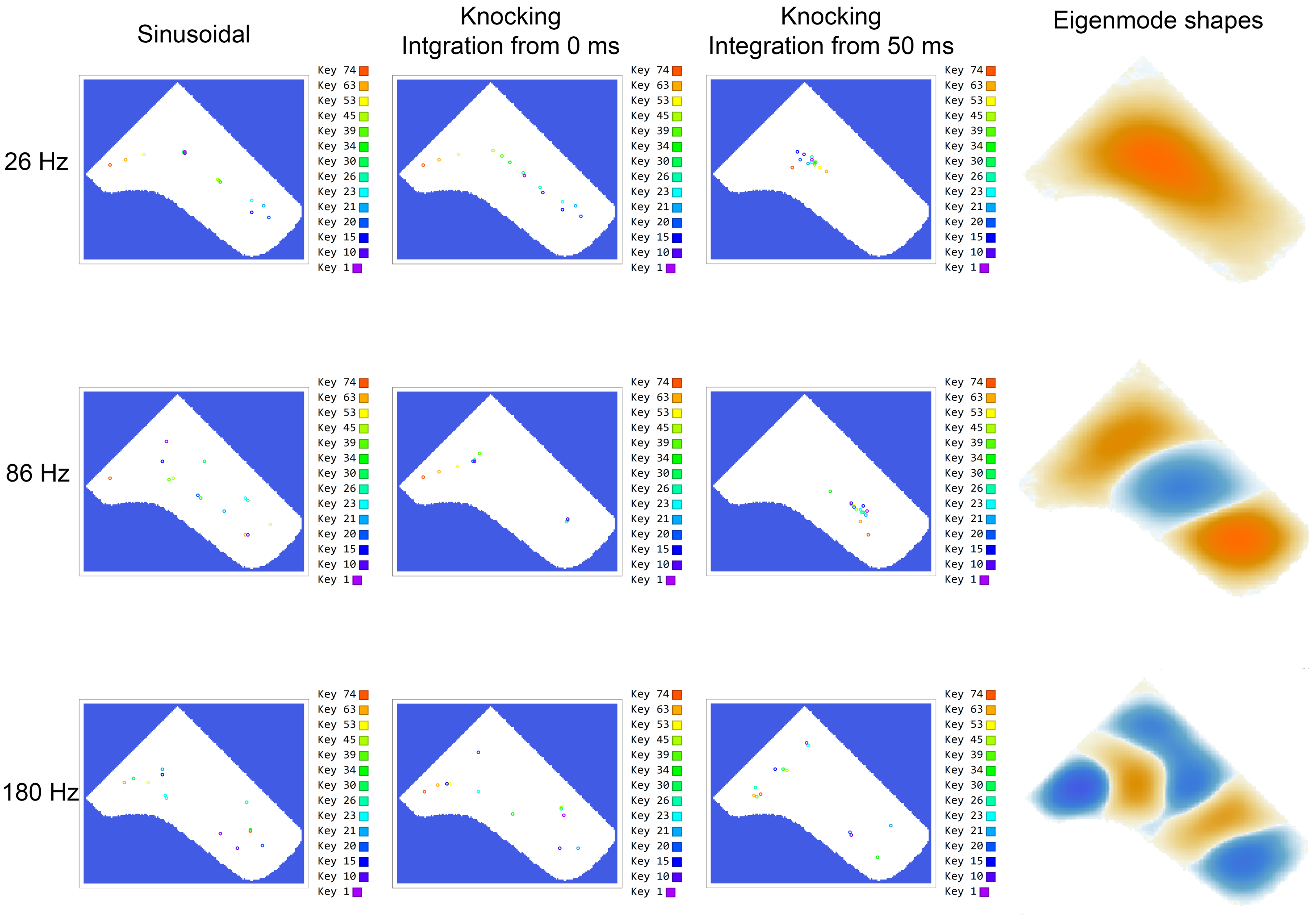
3.2. Forced Oscillation Patterns vs. Eigenmodes

Figure 4 shows the real part of the displacements of the forced oscillations of the simulated soundboard for the different dampings Δ d , and the 14 driving points at 26 Hz sinusoidal driving frequency. As discussed above, three frequencies 26 Hz, 86 Hz, and 180 Hz were chosen, all have three plots, a real-valued, an imaginary-valued, and an absolute amplitude valued plot. Additionally, the driving was sinusoidal and with an impulse, and the analysis of the impact is two-fold, once over one second of sound and once over only the decaying part of the sound 50 ms after the sound onset. Therefore, all together, 27 figures, such as those displayed in Figure 4, are used for the analysis. Due to lack of space, as an example, the lowest frequency driven sinusoidally is shown in its real-valued part. It covers most of the behavior also found with the other plots, which becomes clear in Figure 5 discussed later, which is a summary of all 27 cases.
The rows in Figure 4 show changes of the forced pattern due to increased damping from right to left, where the very right case has a T60 ~ 0.6 s and the very left case a T60 ~ 0.1 s. As indicated in the legend, positive displacements are red, negative are blue, and white indicates zero displacements. Examining, also, the absolute displacements, as well as the phases, not shown here, all patterns are standing waves with nodal lines at the turning points from red to blue and vice versa. All plots are normalized to one.
With all driving points, i.e., in all rows, the driving point has a stronger amplitude and can much more clearly be seen when damping is higher, while with lower damping, the driving point is not so prominent. This is in accordance with the increased damping, as already nicely discussed in [31] Section II. With large damping, the waves leaving the driving point are damped considerably and are, therefore, weaker on all other parts of the plate. This increases the localization of sounds, leaving the soundboard, depending on the piano key played.
When examining only the most left column with highest damping, no eigenmodes are observable. When examining the very right column with low damping, they are much more clearly present. Additionally, the lowest damping values used here show a driving point dependency. At low keys up to about key 34, a relatively stable mode can be observed. At key 34, the driving point is on a nodal line, and, therefore, the pattern is blurred. With higher keys, the pattern changes considerably, depending on the driving point.
In the piano literature, it is usually assumed that the soundboard vibrates in eigenmodes, and when knowing these eigenmodes, all forced oscillations can be calculated by summing the eigenmodes with amplitudes depending on their strength at the driving point [18,32,33,34]. A driving point dependency has been found with harpsichords [35] or guitars [36]. This dependency also holds when driving the soundboards at their eigenfrequencies, displaying considerably different vibration shapes depending on the driving point. One reason for this finding could be damping, as the driving-point dependency can still be calculated analytically for a one-dimensional simple string [37].
Another effect of increasing the damping can be observed at key 34. With low damping, its vibration is low, as a nodal point is used for driving. As eigenmodes seem to disappear with higher damping, this nodal point does no longer play any role. In this case, the vibration is stronger and within the range of all other driving points. Therefore, increasing the damping decreases so-called dead spots on a soundboard, notes which are low in volume.
This is a general and important finding studied before [31,38]. When damping is increased, the eigenmodes disappear. Eigenmodes mean that only those frequencies survive on the soundboard, which are eigenfrequencies of the soundboard. The soundboard is a passive filter that only filters frequencies out and lowers their amplitudes. Filtering happens as the waves caused by a driving frequency that is not an eigenfrequency of the soundboard travel over the soundboard, are reflected at the soundboards’ boundaries, and cancel out due to destructive interference. Still, if the damping of the soundboard is high, or if the boundaries are acoustic black holes with practically no reflections, nearly no such cancellations appear, and no destructive interference of waves happens. Of course, on the other hand, increased damping means a reduction in energy due to the damping. So, when increasing damping, there is a trade-off in energy on the soundboard between increased wave energy due to reduced eigenmodes and decreased wave energy due to internal damping. The former mechanism increases wave amplitudes, the latter reduces them. Now, in cases where the reduced eigenmode filter system has a stronger impact on wave energy than the internal damping, the wave energy on the soundboard increases when increasing the damping. Then, by increasing damping, the radiated sound is louder compared to reduced damping. This seems paradoxical at first that increased internal soundboard damping leads to an increased vibration power. This is an important mechanism when driving the soundboard with frequencies that are not eigenfrequencies of this soundboard, which is considerably the case with lower frequencies. Models so far of an aluminum plate predict up to 8 dB [31], that of a layered plate up to 15 dB sound radiation increase [38]. Heavily damped vibrating systems, such as wood, therefore, are still able to radiate low frequencies that are not eigenfrequencies of the system loud and strong.
Additionally, what is enhanced with increased damping is a homogeneity of sound radiation due to the lack of dead spots and an increased localization due to a strengthening of the amplitudes at the driving points.
The dependency of these findings on the kind of driving the soundboard, as well as for higher frequencies, is shown in Figure 5. Each row represents an eigenfrequency, the top row is 26 Hz, the middle is 86 Hz, and the bottom is 180 Hz. On the very right side, the eigenmodes of these frequencies are shown. As already shown above, eigenmodes depend on damping strength and driving points and may no longer be present at all. Therefore, the shown cases are idle, they are built from the simulations when knocking on the soundboard, cutting off the first 50 ms of the sound, and taking the impact point at a maximum amplitude of the eigenmode. All three frequencies clearly appear as spectral peaks, and, therefore, were used throughout (see Methods section above).
The pictures on the left three columns depict the points of maximum amplitude of the vibrating shape, here coloring represents the impact points. The columns represent different driving mechanisms. The very left column is for sinusoidal driving, the middle and right ones show results when knocking on the plate, the second left column is when integrating the sound over its whole length, the right column is when integrating the sound over its length leaving out the first 50 ms.
All cases are those of minimum damping to show that the effect is still present when damping is at its lowest possible range. All following results sharpen even more when increasing the damping.
The differences are considerable. Examining the 26 Hz case in the highest row, only when knocking and integrating the sound leaving out the initial transient of 50 ms results in an eigenmode shape with maximum amplitudes around the same place on the soundboard. Still, when taking the first 50 ms into consideration of the knocking sound (second plot from left), the driving point in most cases is already the maximum of vibration. This also holds when using a forced sinusoidal oscillation.
This pattern continues when using higher frequencies at 86 Hz (middle row) and 180 Hz (lowest row). As the eigenmode shown on the very right is no longer a monopole, the maximum amplitude of the mode may change in the 180 Hz case. In these cases of 86 Hz and 180 Hz, the driving point dependency is clearly present when knocking and integrating over the whole sound (second column from left), as well as when driving with a sinusoidal force (very left column).
It is striking to see that the mode even for the 26 Hz eigenfrequency of the soundboard changes from a monopole to a dipole when knocking on the soundboard or when driving it with a sinusoidal force, respectively. This can be observed when comparing the eigenmode in Figure 5 (top right plot) to the forced oscillation patterns at 26 Hz in the very right column in Figure 4. This again is an effect of the damping, as can be observed with different driving positions in Figure 4. At higher keys the nodal lines increase from one to two and even to three.
We call these forced oscillation patterns as they are considerably different from eigenmodes and caused by forced oscillations. For a one-dimensional string, the altered mode shapes of the string driven by forced oscillations can still be found analytically [37]. These shapes are very different from the strings’ eigenmodes. However, they also differ from traveling waves, such that there still are nodal points and anti-nodes present. The same reasoning is applied to the piano soundboard to distinguish the soundboard vibration from the eigenmodes, calling these vibrations forced oscillation patterns.
The nodal lines found in forced oscillation patterns present with strong damping need to be at different positions compared to the nodal lines of respective eigenmodes appearing with low damping due to the difference in amplitudes of superposing outgoing and returning waves. A nodal line is a destructive interference of waves at any time. When returning waves are lowered in amplitude, compared to an undamped case, nodal lines will be moved from their position they have in the eigenmode case. The piano soundboard is a very complex geometry, where many reflection points are present. The wave speeds change according to manufacturing stage and boundary conditions [39]. When, e.g., adding a curved bridge, vibration energy is strongly conserved in the bridge bent. The complexity of a piano soundboard is also reflected in the lack of an analytical solution of the bending wave equation with boundary conditions fitting a piano soundboard geometry and the need to calculate this case numerically. Therefore, the striking increase in nodal lines for 26 Hz with increased damping can then be understood as an outcome of complex reflection points together with the considerable amplitude difference between outgoing and returning waves.

4. Conclusions

Several conclusions can be drawn which are expected to hold not only for piano soundboards but for other stringed instruments too.
Increasing the damping tremendously decreases the existence of eigenmode patterns and mainly only leaves the forced oscillation patterns on the soundboard. In the extreme case of no boundary reflections, the soundboard can be considered an infinite plate with no eigenvalues. Such a plate has a flat spectrum, meaning the soundboard does no longer filter the sound of the string acting on it. In such cases, the soundboard does not shape the string sounds any longer but only acts as a radiator of the strings.
On the other extreme, when the soundboard has no damping at all, it is a reverberating plate as known from recording studios with very sharp eigenvalues and eigenmodes and a long reverberating sound. The construction of such a piano soundboard is reported (although without details) to have been tested and not found appropriate as a musical instrument.
Most often, musical instrument soundboards are in between these extremes, shaping the strings sound to some extent while acting as a forced-oscillator on the other. The forced oscillator behavior reduces dead spots on the instrument. It also increases the radiation energy and, therefore, the loudness of the instrument at not-eigenfrequencies of the soundboard, as the filtering of the string’s sound is reduced.
Additionally, it can be expected that the initial transient of a sound is shorter with a heavily damped soundboard. This makes the sound perceptually faster, and the instrument often easier to play.
In terms of the character of the instrument aimed for by instrument makers, as a rule of thumb, one might state that the stronger the internal damping, the more ‘bite’ the instrument has, and the less influence the soundboard has on the instrument sound. The less the internal damping, the longer the sound attack, and the more filtering of the strings appear, leading to more characteristically sounding instruments. The internal damping is, therefore, a design tool for instrument makers, where the choice is up to taste.
Although not investigated in the present paper, this effect could also be enhanced by making the boundaries of the soundboard low in reflection, according to the idea of an acoustic black hole [17].
When following the above findings, one might guess how important the choice of a certain type or quality of wood is for instrument making. Indeed more often than expected, the choice of wood is more driven by a visually beautiful appeal rather than by acoustic testing. Therefore, it might be the case that using different kinds of wood might be counterbalanced by a certain amount of internal damping, achievable by adding varnish or changing the boundaries of sound plates.

Author Contributions

Writing—original draft preparation, R.B. and N.P.; writing—review and editing, R.B. and N.P. All authors have read and agreed to the published version of the manuscript.

Funding

The presented work has been funded by the Deutsche Forschungsgemeinschaft (DFG).

Data Availability Statement

Not applicable.

Acknowledgments

The authors thank Florian Pfeifle and Christian Koehn for helping with the measurements.

Conflicts of Interest

The authors declare no conflict of interest.

References

  1. Pierce, A. Intrinsic damping, relaxation processes, and internal friction in vibrating systems. POMA 2010, 9, 1–16. [Google Scholar]
  2. Norris, A.N.; Photiadis, D.M. Thermoelastic Relaxation in Elastic Structures, with Applications to Thin Plates. arXiv 2004, arXiv:cond-mat/0405323v2. [Google Scholar]
  3. French, A.D.; Johnson, G.P. Advanced conformational energy surfaces for cellobiose. Cellulose 2004, 11, 449–462. [Google Scholar] [CrossRef]
  4. Tramer, A.; Jungen, C.; Lahmani, F. Energy Dissipation in Molecular Systems; Springer: Heidelberg, Germany, 2005. [Google Scholar]
  5. Zhou, X.Q.; Yu, D.Y.; Shao, X.Y.; Zhang, S.Q.; Wang, S. Research and applications of viscoelastic vibration damping materials: A review. Compos. Struct. 2016, 135, 460–480. [Google Scholar] [CrossRef]
  6. Zhou, X.Y.; Yu, D.Y.; Shao, X.Y.; Wang, S.; Tian, Y.H. Asymptotic analysis on flexural dynamic characteristics for a sandwich plate with periodically perforated viscoelastic damping material core. Compos. Struct. 2015, 119, 487–504. [Google Scholar] [CrossRef]
  7. Zhou, X.Q.; Yu, D.Y.; Shao, X.; Wang, S.; Tian, Y.H. Band gap characteristics of periodically stiffened-thin-plate based on center-finite-difference-method. Thin-Walled Struct. 2014, 82, 115–123. [Google Scholar] [CrossRef]
  8. Brémaud, I. What do we know on “resonance wood” properties? Selective review and ongoing research. In Proceedings of the Acoustics 2012 Nantes Conference, Nantes, France, 23–27 April 2012. [Google Scholar]
  9. Brémaud, I.; Gril, J.; Thibaut, B. Anisotropy of wood vibrational properties: Dependence on grain angle and review of literature data. Wood Sci. Technol. 2011, 45, 735–754. [Google Scholar] [CrossRef]
  10. Brémaud, I.; Ruelle, J.; Thibaut, A.; Thibaut, B. Changes in viscoelastic vibrational properties between compression and normal wood: Roles of microbril angle and of lignin. Holzforschung 2013, 67, 75–85. [Google Scholar] [CrossRef] [Green Version]
  11. Obataya, E.; Umezawa, T.; Nakatsubo, F.; Norimoto, M. The effects of water soluble extractives on the acoustics properties of reed (Arundo donax L.). Holzforschung 1999, 53, 63–67. [Google Scholar] [CrossRef]
  12. Schleske, M. On the Acoustical Properties of Violin Varnish. CAS 1998, 3, 27–43. [Google Scholar]
  13. Romanillos, J.L. Antonio De Torres: Guitar Maker-His Life and Work; Yehudi Menuhin music guides; Bold Strummer Ltd.: Westport, CT, USA, 1997. [Google Scholar]
  14. Hansing, S. Das Pianoforte und seine akustischen Anlagen [The Pianoforte and Its Acoustical Properties]; Im Selbstverlage des Verfassers: Schwerin, Germany, 1910. [Google Scholar]
  15. Bilhuber, P.H. Diaphragm Unit and Method of Fabricating Same. U.S. Patent No. 2,529,862, 14 November 1950. [Google Scholar]
  16. Bilhuber, P.H.; Johnson, C.A. The Influence of the Soundboard on Piano Tone Quality. J. Acoust. Soc. Am. 1940, 11, 311–320. [Google Scholar] [CrossRef]
  17. Conlona, S.C.; Fahnline, J.B. Numerical analysis of the vibroacoustic properties of plates with embedded grids of acoustic black holes. J. Acoust. Soc. Am. 2015, 137, 447–457. [Google Scholar] [CrossRef] [PubMed]
  18. Adrien Mamou-Mani, J.F.; Besnainou, C. Numerical simulation of a piano soundboard under downbearing. J. Acoust. Soc. Am. 2008, 123, 2401–2406. [Google Scholar] [CrossRef] [PubMed]
  19. Mamou-Mani, A.; Moyne, S.L.; Ollivier, F.; Besnainou, C.; Frelat, J. Prestress effects on the eigenfrequencies of the soundboards: Experimental results on a simplified string instrument. J. Acoust. Soc. Am. 2012, 131, 872–877. [Google Scholar] [CrossRef] [PubMed]
  20. Petersen, S. Craftsmen- Turned- Scientists? The Circulation of Explicit and Working Knowledge in Musical- Instrument Making, 1880–1960. OSIRIS 2013, 28, 212–231. [Google Scholar] [CrossRef]
  21. Chaigne, A.; Lambourg, C. Time-domain simulation of damped impacted plates. I. Theory and experiments. J. Acoust. Soc. Am. 2001, 109, 1422–1432. [Google Scholar] [CrossRef]
  22. Lambourg, C.; Chaigne, A.; Matignon, D. Time-domain simulation of damped impacted plates. II. Numerical model and results. J. Acoust. Soc. Am. 2001, 109, 1433–1447. [Google Scholar] [CrossRef] [Green Version]
  23. Bader, R. Computational Mechanics of the Classical Guitar; Springer: Berlin/Heidelberg, Germany, 2005. [Google Scholar]
  24. Bader, R. Finite-Difference model of mode shape changes of the Myanmar pat wain drum circle using tuning paste. Proc. Mtgt. Acoust. 2016, 29, 035004. [Google Scholar]
  25. Schroeder, M.R. New Method of Measuring Reverberation Time. J. Acoust. Soc. Am. 1965, 37, 409. [Google Scholar] [CrossRef]
  26. Farina, A. Simultaneous measurement of impulse response and distortion with a swept-sine technique. In Proceedings of the Audio Engineering Society Convention 108, Paris, France, 19–22 February 2000; pp. 1–24. [Google Scholar]
  27. Plath, N.; Pfeifle, F.; Koehn, C.; Bader, R. Radiation Characteristics of Grand Piano Soundboards in Different Stages of Production. In Proceedings of the 2017 International Symposium on Musical Acoustics, Montreal, QC, Canada, 18–22 June 2017. [Google Scholar]
  28. Plath, N.; Pfeifle, F.; Koehn, C.; Bader, R. Driving Point Mobilities of a Concert Grand Piano Soundboard in Different Stages of Production. In Proceedings of the 3rd Annual COST FP1302 WoodMusICK Conference, Barcelona, Spain, 7–9 September 2016; pp. 117–123. [Google Scholar]
  29. Lawergren, B. Acoustics and Evoluation of Arched Harps. Galpin Soc. J. 1981, 34, 110–129. [Google Scholar] [CrossRef]
  30. Williamson, M. The Burmese Harp: Its Classical Music, Tunings, & Modes; Northern Illinois Monograph Series of Southeast Asia; Northern Illinois University: DeKalb, IL, USA, 2000; Volume 1. [Google Scholar]
  31. Koe, Y.; Liu, B.; Tian, J. Radiation efficiency of damped plates. J. Acoust. Soc. Am. 2015, 137, 1032–1035. [Google Scholar] [CrossRef] [PubMed]
  32. Giordano, N. Simple model of a piano soundboard. J. Acoust. Soc. Am. 1997, 102, 1159–1168. [Google Scholar] [CrossRef]
  33. Moore, T.R.; Zietlow, S.A. Interferometric studies of a piano soundboard. JASA 2006, 119, 1783–1793. [Google Scholar] [CrossRef] [PubMed] [Green Version]
  34. Mokdat, F. Fully Parameterized Finite Element Model of a Grand Piano Soundboard for Sensitivity Analysis of the Dynamic Behavior. Ph.D. Thesis, University of Arizona, Tucson, AZ, USA, 2013. [Google Scholar]
  35. Beurmann, A.; Bader, R.; Schneider, A. An acoustical study of a Kirkman harpsichord from 1766. Galpin Soc. J. 2010, 63, 61–72. [Google Scholar]
  36. Bader, R. Nonlinearities and Synchronization in Musical Acoustics and Music Psychology; Current Research in Systematic Musicology; Springer: Berlin/Heidelberg, 2013; Volume 2, pp. 157–284. [Google Scholar]
  37. Fahy, F. Sound and Structural Vibration: Radiation, Transmission and Response, 2nd ed.; Elsevier: Amsterdam, The Netherlands, 2007. [Google Scholar]
  38. Loredo, A.; Plessy, A.; Hafidi, A.E.; Hamzaoui, N. Numerical vibroacoustic analysis of plates with constrained-layer damping patches. J. Acoust. Soc. Am. 2011, 129, 1905–1918. [Google Scholar] [CrossRef]
  39. Plath, N. From Workshop to Concert Hall: Acoustic Observations on a Gran Piano under Construction. Ph.D. Thesis, University of Hamburg, Hamburg, Germany, 2019. [Google Scholar]
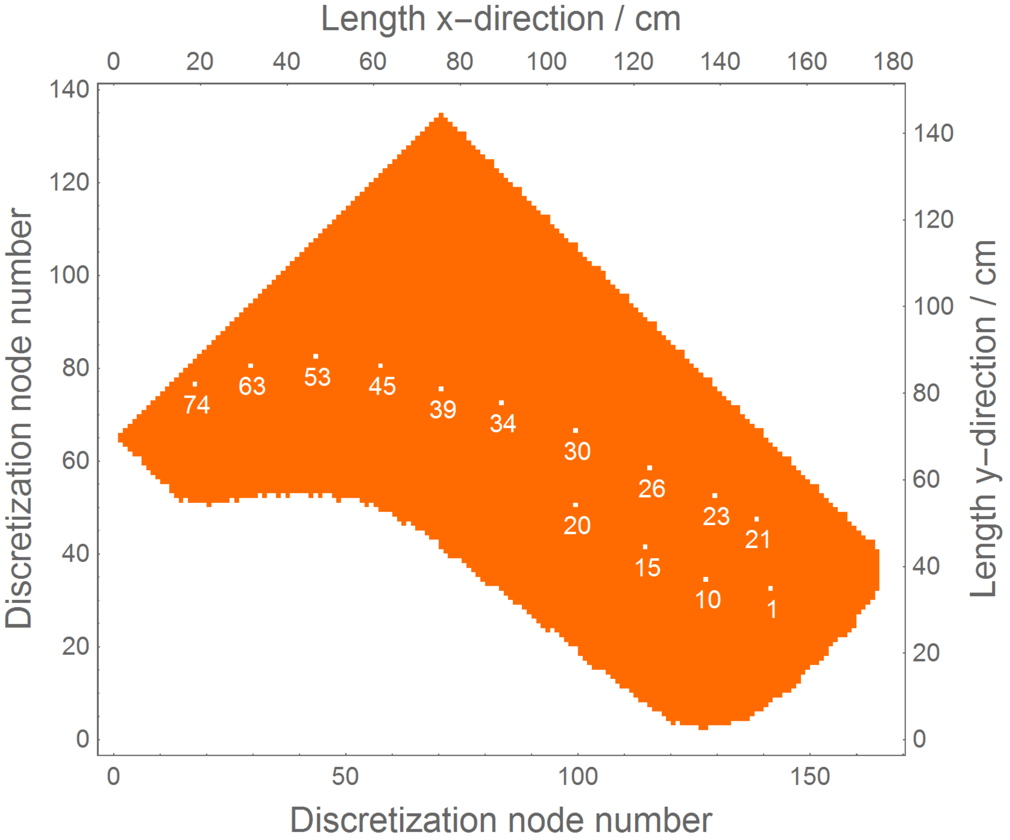
Figure 1. Discrete soundboard geometry of a grand piano showing the amount of grid points used in the discrete FDTD model. The points on the geometry indicate the driving points corresponding to the key numbers of the strings acting on the soundboard.
Acoustics 04 00062 g001
Figure 2. Measured T60 decay times for a piano soundboard in two production stages at 14 string/bridge impact points. Circles indicate mean values over all microphone recordings, triangles represent (mean ± standard deviation). (Left) the raw soundboard, (right) the finished soundboard. At the very first stage of production (left) T60 ~ 0.3, while after gluing the soundboard to the piano rim (right) T60 raises up to T60 ~ 0.6 s.
Acoustics 04 00062 g002
Figure 3. T60 of knocking sounds on 14 impact positions at the piano bridge for nine damping strength as used in the simulation, with decreasing strength from left to right. The measured T60 of the raw piano soundboard is around T60 ~ 0.3 s, the T60 for the finished soundboard are around T60 ~ 0.6 s. Therefore, the displayed range is up to the maximum damping of regular piano soundboards. The minimum damping is decreased to below T60 ~ 0.1 s to show the impact of damping on soundboards.
Acoustics 04 00062 g003
Figure 4. Real valued amplitudes of the FDM raw soundboard simulation, driven sinusoidally with 26 Hz at 14 impact points at bridge positions and simulating with nine damping strength values with decreasing damping from right to left. The very left column, therefore, represents the forced oscillation patterns for maximum damping used. The maximum amplitudes of the patterns follow the impact point of driving the soundboard. Leaving the respective impact points leads to a decrease in amplitude of a traveling wave. Each row of the plot shows the change of this pattern when decreasing the damping. With decreased damping, modal patterns appear gradually more and more. Still, even with minimum damping at the very right of the plot, the modal patterns of different impact points are considerably different. Therefore, a certain damping leads to a mixture of the eigenmode with a pattern emphasizing the impact point.
Acoustics 04 00062 g004
Figure 5. Positions of maximum absolute amplitudes on a raw piano soundboard (first three columns) for 14 driving points (colors) for three different frequencies, top row: 26 Hz, middle row: 86 Hz, bottom row: 180 Hz, with respective modal shapes displayed in the very right column. The left three columns show the maximum amplitude positions for three different conditions: sinusoidal driving (left column), knocking with integration of sound from the very start (second left column), and knocking with integration of sound starting 50 ms after knocking onset. In all cases, the simulation case with minimal damping is displayed. With all three frequencies the very left column shows maximum amplitude positions following the impact positions, where the lowest frequency of 26 Hz follows most clearly. When knocking on the top plate with integration of sound from the very start (second left column), a similar behavior can be seen. Still, when knocking and integrating only after 50 ms after knocking (second right column), the maximum points follow eigenmode patterns, again most clear with 26 Hz and less with higher frequencies. Therefore, eigenmode patterns do appear with piano soundboards, still, when driven with forced oscillations, the vibrational patterns also follow the impact point.
Acoustics 04 00062 g005
Table 1. Positions of impact points on the raw piano soundboard with respective keys.
Key110152021232630343945536374
x-positon/mm39553059064527032040048559168078089510551220
y-position/mm17301570137511301560140012009657355603752259515
Publisher’s Note: MDPI stays neutral with regard to jurisdictional claims in published maps and institutional affiliations.

