
On the Robustness and Efficiency of the Plane-Wave-Enriched FEM with Variable q-Approach on the 2D Room Acoustics Problem


Abstract
:1. Introduction
1.1. Background
1.2. Study Purpose
2. Theory
2.1. Discretization of the Closed Sound Field Using Plane-Wave-Enriched FEM
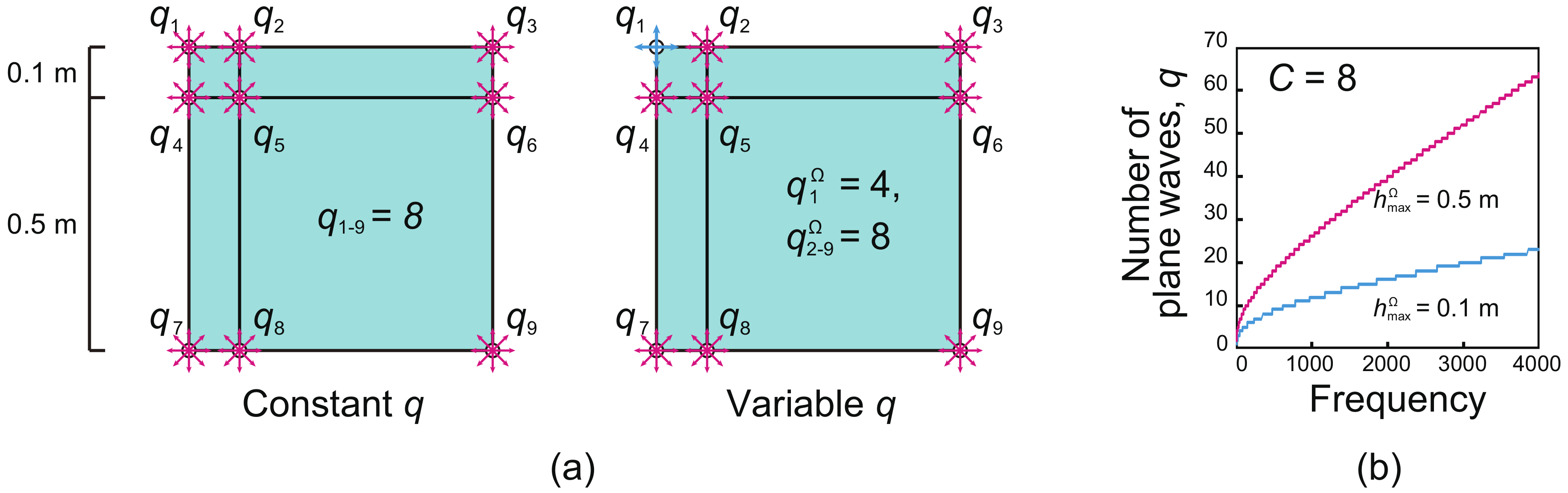
2.2. Setup of the Plane-Wave Number for q-Refinement
3. Numerical Experiments
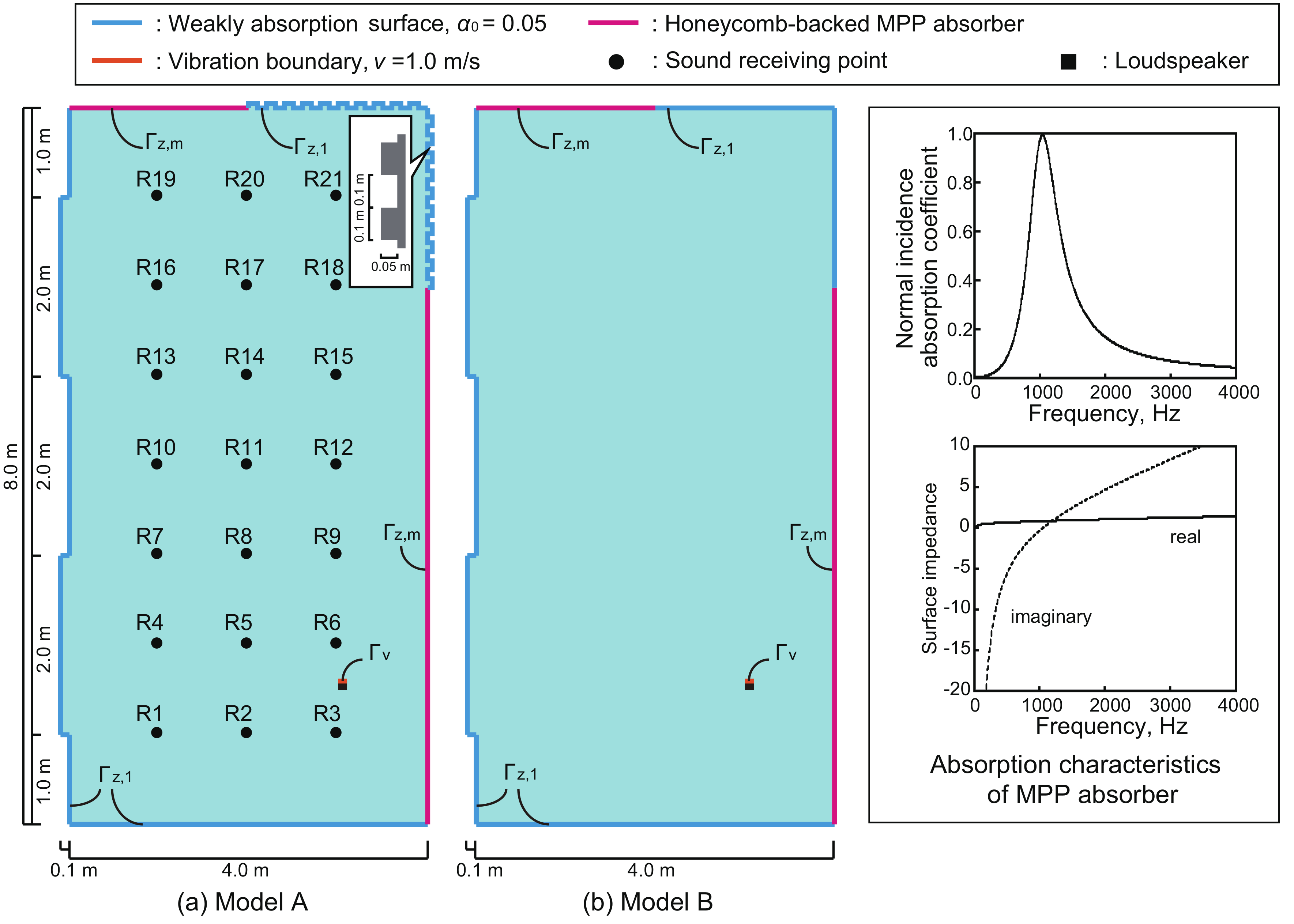
3.1. Problem Description and Numerical Setup
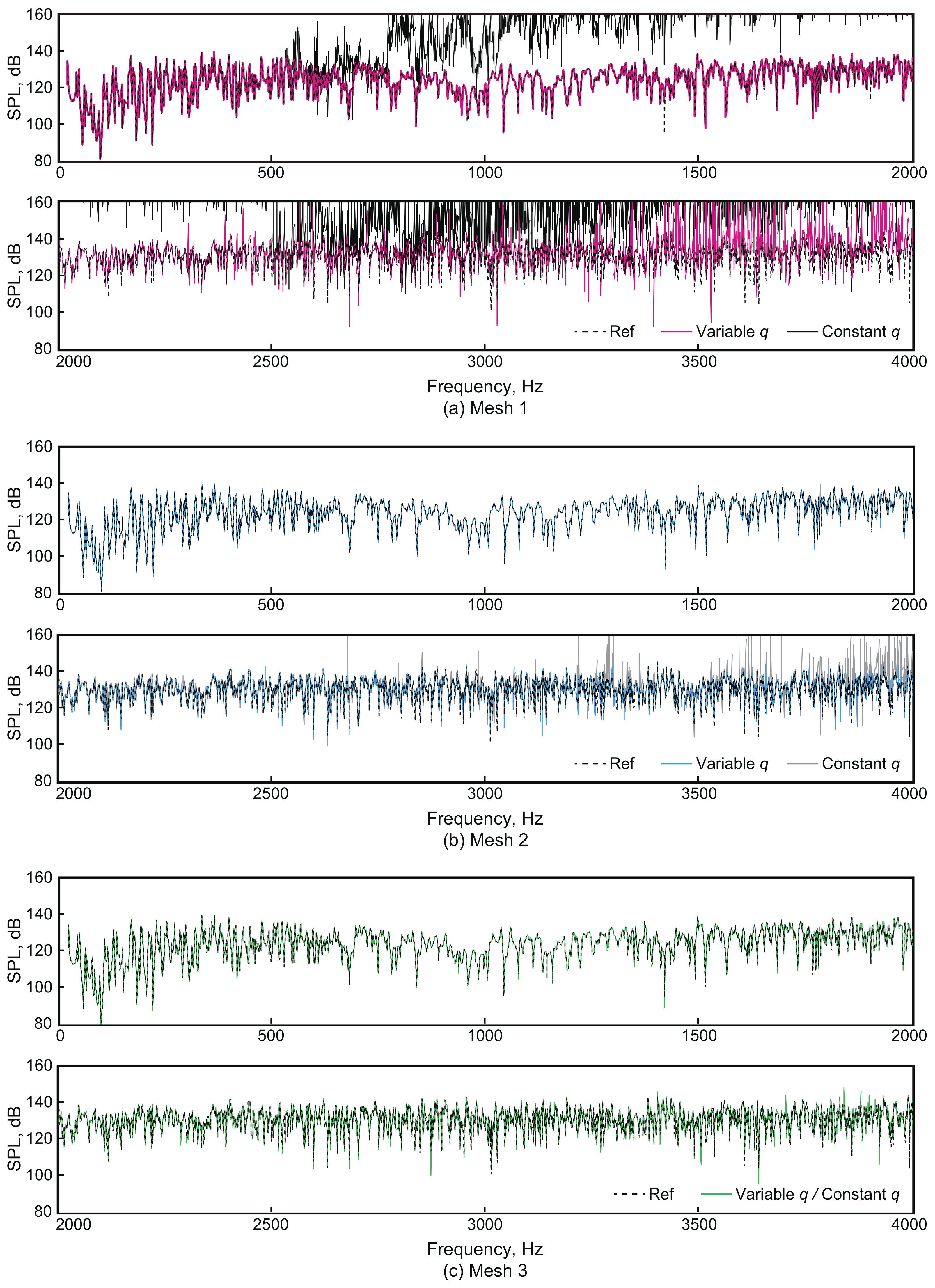
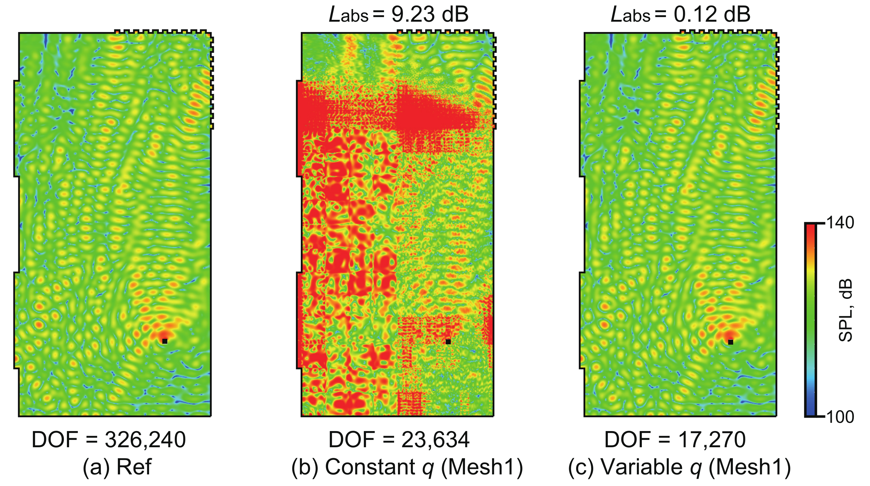
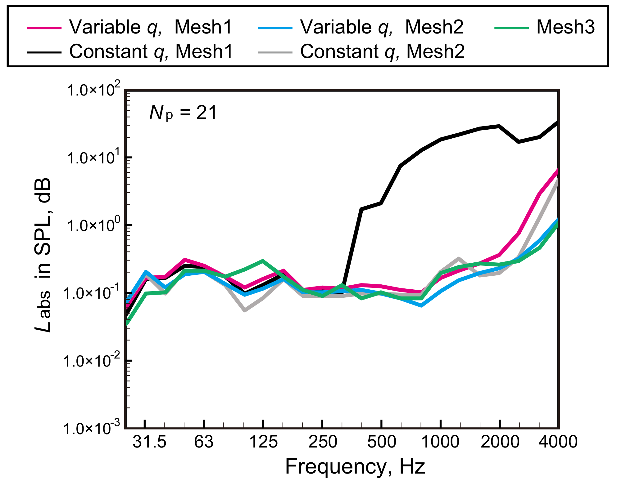
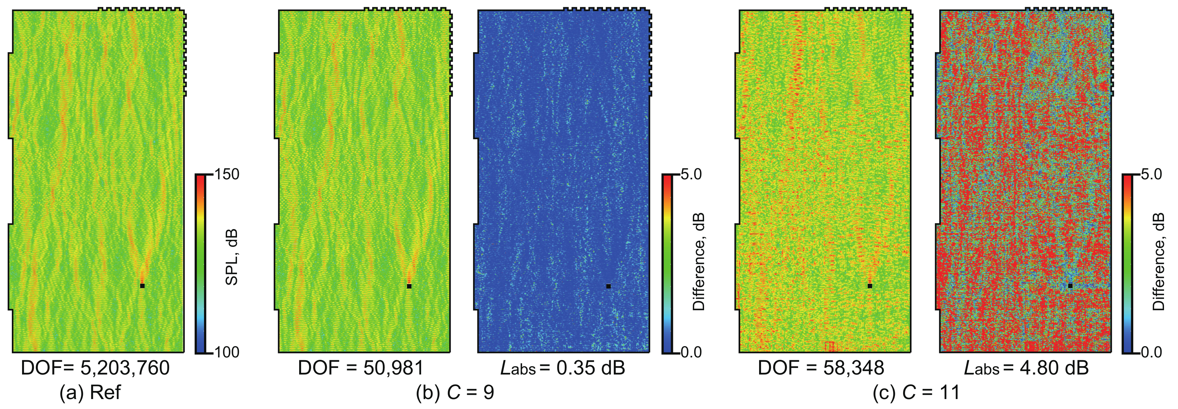
3.2. Effectiveness of the Variable q-Approach against the Constant q-Approach
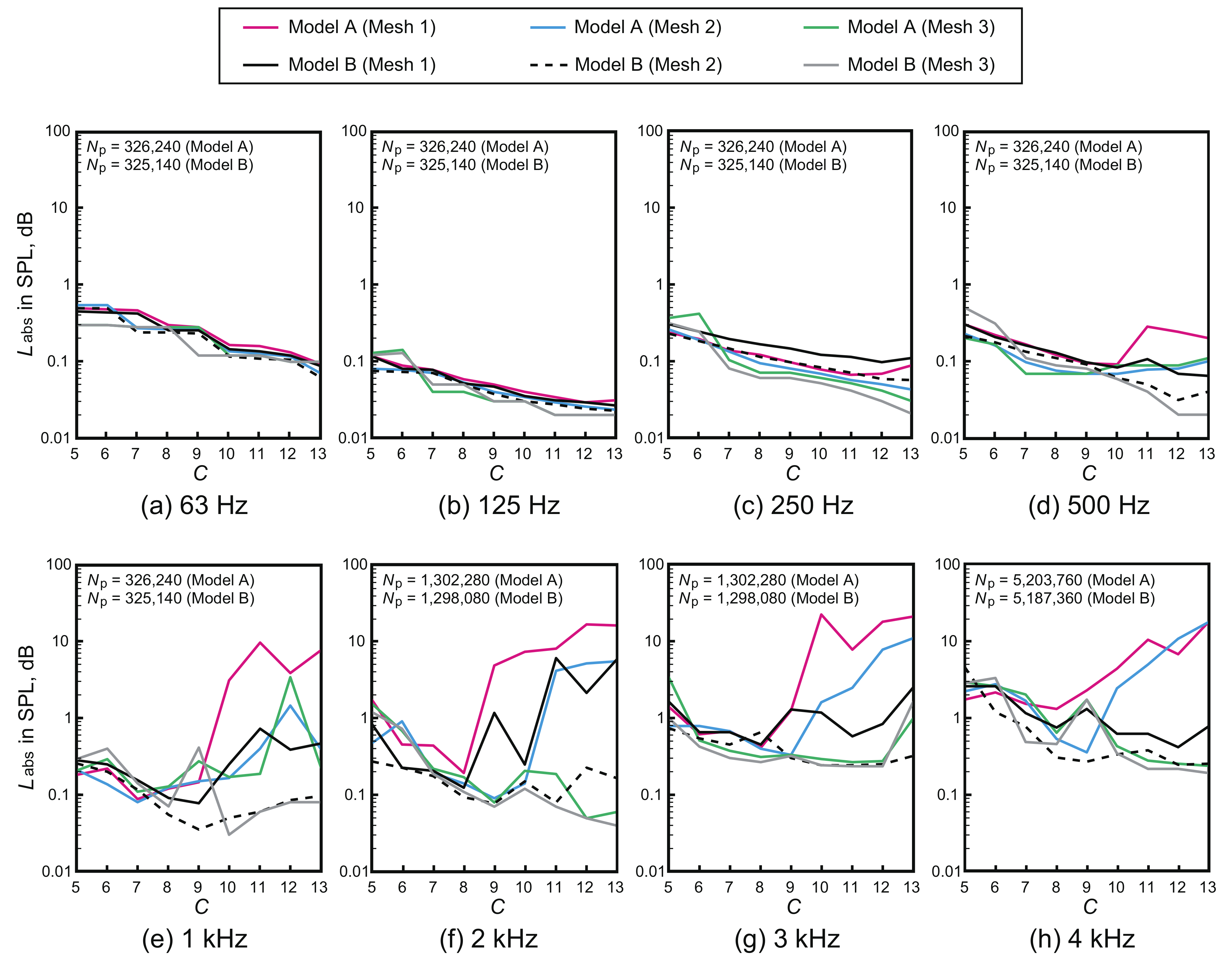
3.3. Mesh and Room Geometry Effects on the Robustness of the PW-FEM Using the Variable q-Approach
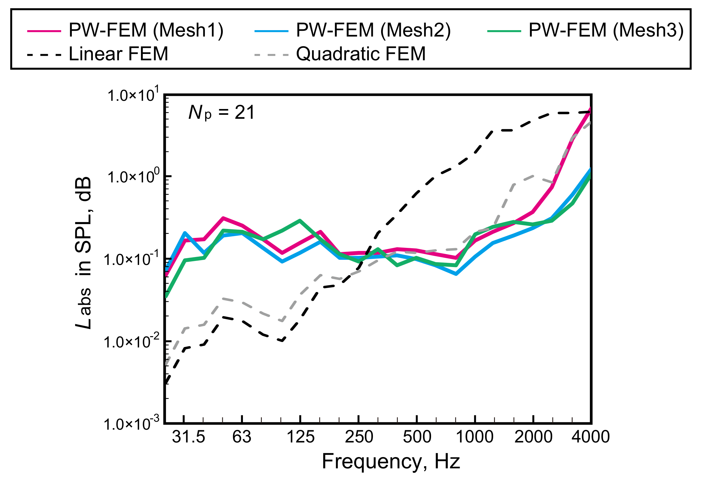
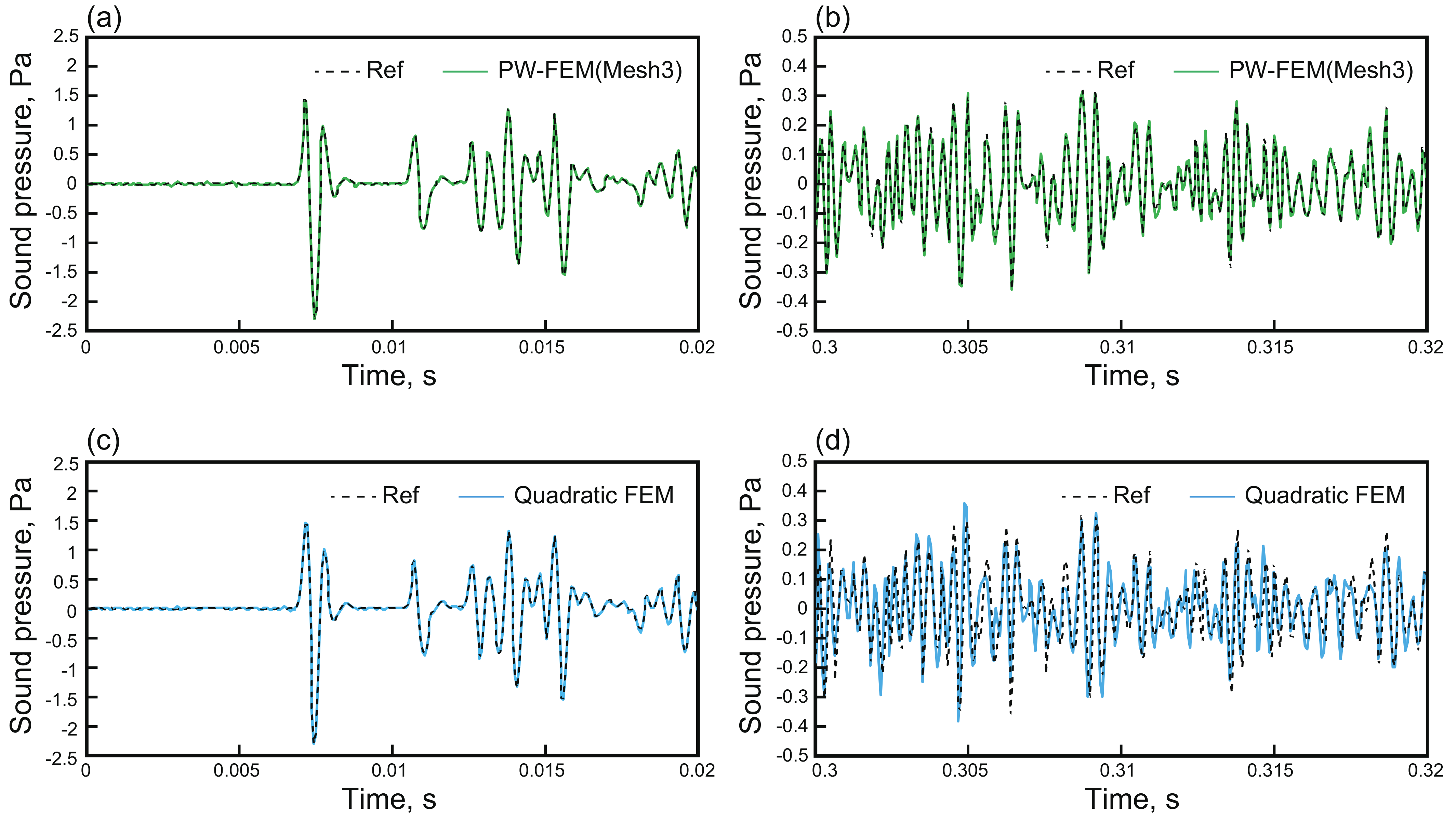
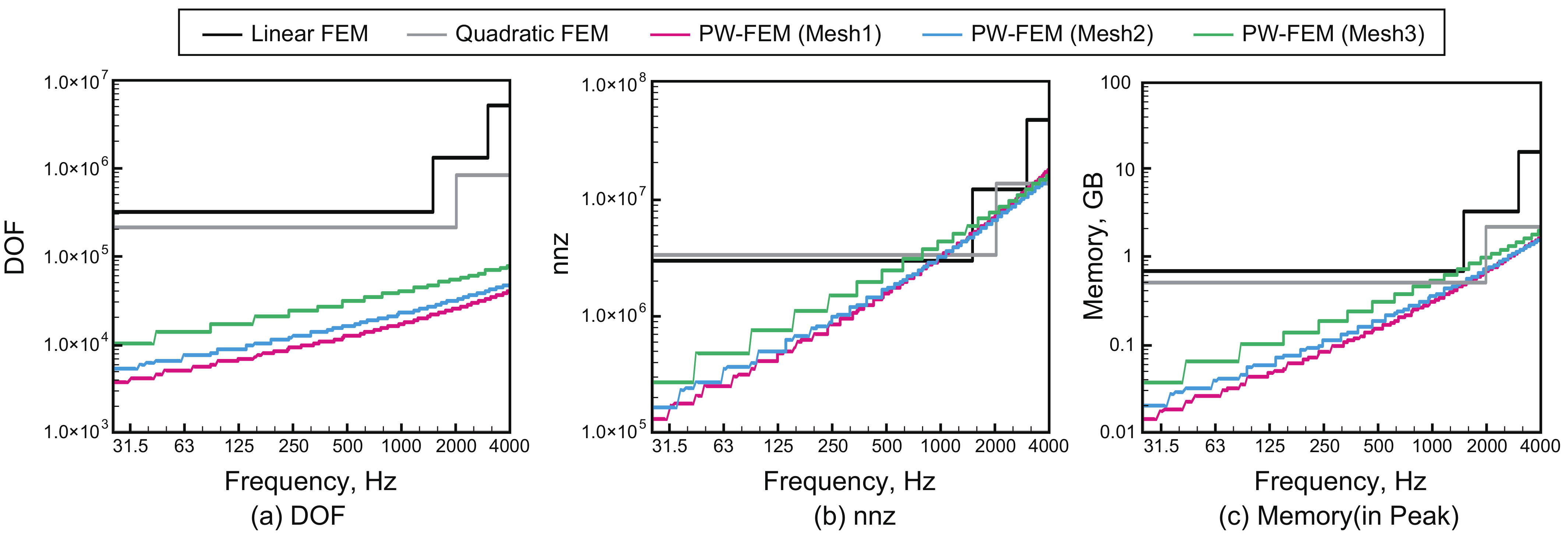
3.4. Performance Comparison with Classical Linear and Quadratic FEMs
4. Conclusions
Author Contributions
Funding
Institutional Review Board Statement
Informed Consent Statement
Data Availability Statement
Acknowledgments
Conflicts of Interest
References
- Savioja, L.; Svensson, U.P. Overview of geometrical room acoustic modeling techniques. J. Acous. Soc. Am. 2015, 138, 708–730. [Google Scholar] [CrossRef] [Green Version]
- Sakuma, T.; Sakamoto, S.; Otsuru, T. (Eds.) Computational Simulation in Architectural and Environmental Acoustics—Methods and Applications of Wave-Based Computation; Springer: Tokyo, Japan, 2014. [Google Scholar]
- Okuzono, T.; Otsuru, T.; Tomiku, R.; Okamoto, N. A finite element method using dispersion reduced spline elements for room acoustics simulation. Appl. Acoust. 2014, 79, 1–8. [Google Scholar] [CrossRef] [Green Version]
- Botteldooren, D. Finite-difference time-domain simulation of low-frequency room acoustics problems. J. Acoust. Soc. Am. 1995, 98, 3302–3308. [Google Scholar] [CrossRef]
- Otsuru, T.; Okamoto, N.; Okuzono, T.; Sueyoshi, T. Applications of large-scale finite element sound field analysis onto room acoustics. In Proceedings of the 19th International Congress on Acoustics, Madrid, Spain, 2–7 September 2007. [Google Scholar]
- Okamoto, N.; Tomiku, R.; Otsuru, T.; Yasuda, Y. Numerical analysis of large-scale sound fields using iterative methods part II: Application of Krylov subspace methods to finite element analysis. J. Comput. Acoust. 2007, 15, 473–493. [Google Scholar] [CrossRef]
- Aretz, M.; Vorländer, M. Combined wave and ray based room acoustic simulations of audio systems in car passenger compartments, Part II: Comparison of simulations and measurements. Appl. Acoust. 2014, 76, 52–65. [Google Scholar] [CrossRef]
- Okuzono, T.; Sakagami, K. A frequency domain finite element solver for acoustic simulations of 3D rooms with microperforated panel absorbers. Appl. Acoust. 2018, 129, 1–12. [Google Scholar] [CrossRef] [Green Version]
- Hoshi, K.; Hanyu, T.; Okuozno, T.; Sakagami, K.; Yairi, M.; Harada, S.; Takahashi, S.; Ueda, Y. Implementation experiment of a honeycomb-backed MPP sound absorber in a meeting room. Appl. Acoust. 2020, 157, 107000. [Google Scholar] [CrossRef]
- Yasuda, Y.; Ueno, S.; Kadota, M.; Sekine, H. Applicability of locally reacting boundary conditions to porous material layer backed by rigid wall: Wave-based numerical study in non-diffuse sound field with unevenly distributed sound absorbing surfaces. Appl. Acoust. 2016, 113, 45–57. [Google Scholar] [CrossRef]
- Yasuda, Y.; Saito, K.; Sekine, H. Effects of the convergence tolerance of iterative methods used in the boundary element method on the calculation results of sound fields in rooms. Appl. Acoust. 2020, 157, 106997. [Google Scholar] [CrossRef]
- Sakamoto, S. Phase-error analysis of high-order finite-difference time-domain scheme and its influence on calculation results of impulse response in closed sound field. Acoust. Sci. Technol. 2007, 28, 295–309. [Google Scholar] [CrossRef] [Green Version]
- Kowalczyk, K.; Walstijn, M. Formulation of locally reacting surfaces in FDTD/K-DWM modelling of acoustic spaces. Acta Acust. United Acust. 2008, 94, 891–906. [Google Scholar] [CrossRef] [Green Version]
- Kowalczyk, K.; Van Walstijn, M. Room Acoustics Simulation Using 3-D Compact Explicit FDTD Schemes. IEEE Trans. Audio Speech Lang. Process. 2010, 19, 4–46. [Google Scholar] [CrossRef] [Green Version]
- Sakamoto, S.; Nagatomo, H.; Ushiyama, A.; Tachibana, H. Calculation of impulse responses and acoustic parameters in a hall by the finite-difference time-domain method. Acoust. Sci. Technol. 2008, 29, 256–265. [Google Scholar] [CrossRef] [Green Version]
- Hamilton, B.; Bilbao, S. FDTD methods for 3-D room acoustics simulation with high-order accuracy in space and time. IEEE Trans. Audio Speech Lang. Process. 2017, 25, 2112–2124. [Google Scholar] [CrossRef]
- Okuzono, T.; Otsuru, T.; Tomiku, R.; Okamoto, N. Fundamental accuracy of time domain finite element method for sound field analysis of rooms. Appl. Acoust. 2010, 71, 940–946. [Google Scholar] [CrossRef] [Green Version]
- Okuzono, T.; Yoshida, T.; Sakagami, K.; Otsuru, T. An explicit time-domain finite element method for room acoustics simulations: Comparison of the performance with implicit methods. Appl. Acoust. 2015, 104, 76–84. [Google Scholar] [CrossRef]
- Okuzono, T.; Shimizu, N.; Sakagami, K. Predicting absorption characteristics of single-leaf permeable membrane absorbers using finite element method in a time domain. Appl. Acoust. 2019, 151, 172–182. [Google Scholar] [CrossRef]
- Bilbao, S. Modeling of Complex Geometries and Boundary Conditions in Finite Difference/Finite Volume Time Domain Room Acoustics Simulation. IEEE Trans. Audio Speech Lang. Process. 2013, 21, 1524–1533. [Google Scholar] [CrossRef] [Green Version]
- Bilbao, S.; Hamilton, B.; Botts, J.; Savioja, L. Finite volume time domain room acoustics simulation under general impedance boundary conditions. IEEE Trans. Audio Speech Lang. Process. 2016, 24, 161–173. [Google Scholar] [CrossRef] [Green Version]
- Hornikx, M.; Hak, C.; Wenmaekers, R. Acoustic modelling of sports halls, two case studies. J. Build. Perform. Simul. 2015, 8, 26–38. [Google Scholar] [CrossRef] [Green Version]
- Hornikx, M.; Krijnen, T.; van Harten, L. openPTSD: The open source pseudo-spectral time-domain method for acoustic propagation. Comput. Phys. Commun. 2016, 203, 298–308. [Google Scholar] [CrossRef]
- Simonaho, S.P.; Lähivaara, T.; Huttunen, T. Modeling of acoustic wave propagation in time-domain using the discontinuous Galerkin method—A comparison with measurements. Appl. Acoust. 2012, 73, 173–183. [Google Scholar] [CrossRef]
- Wang, H.; Sihar, I.; Pagán, Muńoz, R.; Hornikx, M. Room acoustics modelling in the time-domain with the nodal discontinuous Galerkin method. Acoust. Soc. Am. 2019, 145, 2650–2663. [Google Scholar] [CrossRef] [PubMed] [Green Version]
- Wang, H.; Hornikx, M. Time-domain impedance boundary condition modeling with the discontinuous Galerkin method for room acoustics simulations. J. Acoust. Soc. Am. 2020, 147, 2534–2546. [Google Scholar] [CrossRef] [PubMed]
- Pind, F.; Jeong, C.H.; Hesthaven, J.S.; Engsig-Karup, A.P.; Strømann-Andersen, J. A phenomenological extended-reaction boundary model for time-domain wave-based acoustic simulations under sparse reflection conditions using a wave splitting method. Appl. Acoust. 2021, 172, 107596. [Google Scholar] [CrossRef]
- Mehra, R.; Raghuvanshi, N.; Savioja, L.; Lin, M.C.; Manocha, D. An efficient GPU-based time domain solver for the acoustic wave equation. Appl. Acoust. 2012, 73, 83–94. [Google Scholar] [CrossRef] [Green Version]
- Rabisse, K.; Ducourneau, J.; Faiz, A.; Trompette, N. Numerical modelling of sound propagation in rooms bounded by walls with rectangular irregularities and frequency-dependent impedance. J. Sound Vib. 2019, 440, 291–314. [Google Scholar] [CrossRef]
- Melenk, J.M.; Babuška, I. Partition of unity finite element method: Basic theory and applications. Comput. Methods Appl. Mech. Eng. 1996, 139, 289–314. [Google Scholar] [CrossRef] [Green Version]
- Babuška, I.; Melenk, J.M. The partition of unity method. Int. J. Numer. Meth. Eng. 1997, 40, 727–758. [Google Scholar] [CrossRef]
- Laghrouche, O.; Mohamed, M.S. Locally enriched finite elements for the Helmholtz equation in two dimensions. Comput. Struct. 2010, 88, 469–1473. [Google Scholar] [CrossRef]
- Mohamed, M.S.; Laghrouche, O.; El-Kacimi, A. Some numerical aspects of the PUFEM for efficient solution of 2D Helmholtz problems. Comput. Struct. 2010, 88, 1484–1491. [Google Scholar] [CrossRef]
- Mohamed, M.S. Numerical Aspects of the PUFEM for Efficient Solution of Helmholtz Problems. Ph.D. Thesis, Heriot–Watt University, Edinburgh, UK, 2010. [Google Scholar]
- Dinachandra, M.; Raju, S. Plane wave enriched Partition of Unity Isogeometric Analysis (PUIGA) for 2D-Helmholtz problems. Comput. Methods Appl. Mech. Eng. 2018, 335, 380–402. [Google Scholar] [CrossRef]
- Diwan, G.C.; Mohamed, M.S. Pollution studies for high order isogeometric analysis and finite element for acoustic problems. Comput. Methods Appl. Mech. Eng. 2019, 350, 701–718. [Google Scholar] [CrossRef]
- Okuzono, T.; Mohamed, M.S.; Sakagami, K. Potential of room acoustic solver with plane-wave-enriched finite element method. Appl. Sci. 2020, 10, 1969. [Google Scholar] [CrossRef] [Green Version]
- Chazot, J.D.; Nennig, B.; Perrey-Debain, E. Performances of the partition of unity finite element method for the analysis of two-dimensional interior sound fields with absorbing materials. J. Sound Vib. 2013, 332, 1918–1929. [Google Scholar] [CrossRef]
- Chazot, J.D.; Perrey-Debain, E. The partition of unity finite element method for the simulation of waves in air and poroelastic media. J. Acoust. Soc. Am. 2014, 135, 724–733. [Google Scholar] [CrossRef] [Green Version]
- Tamaru, K.; Okuzono, T.; Mukae, S.; Sakagami, K. Exploration of efficient numerical integration rule for wide-band room-acoustics simulations by plane-wave-enriched finite-element method. Acoust. Sci. Technol. 2020, 42, 231–240. [Google Scholar] [CrossRef]
- Hiptmair, R.; Moiola, A.; Perugia, I. Survey of Trefftz methods for the Helmholtz equation. In Building Bridges: Connections and Challenges in Modern Approaches to Numerical Partial Differential Equations; Springer: Cham, Switzerland, 2016; pp. 237–278. [Google Scholar]
- Mukae, S.; Okuzono, T.; Tamaru, K.; Sakagami, K. Modeling microperforated panels and permeable membranes for a room acoustic solver with plane-wave-enriched FEM. Appl. Acoust. 2022, 185, 108383. [Google Scholar] [CrossRef]
- Maa, D.Y. Microperforated-panel wideband absorbers. Noise Control Eng. J. 1987, 29, 77–84. [Google Scholar] [CrossRef]
- Sakagami, K.; Funahashi, K.; Somatomo, Y.; Okuzono, T.; Nishikawa, C.; Toyoda, M. An experimental study on the absorption characteristics of a three-dimensional permeable membrane space sound absorber. Noise Control Eng. J. 2015, 63, 300–307. [Google Scholar] [CrossRef] [Green Version]
- Craggs, A. A finite element model for rigid porous absorbing materials. J. Sound Vib. 1978, 61, 101–111. [Google Scholar] [CrossRef]
- Craggs, A. Coupling of finite element acoustic absorption models. J. Sound Vib. 1979, 66, 605–613. [Google Scholar] [CrossRef]
- Easwaran, V.; Munjal, M.L. Finite element analysis of wedges used in anechoic chambers. J. Sound Vib. 1993, 160, 333–350. [Google Scholar] [CrossRef]
- Allard, J.F.; Atalla, N. Sound propagation in porous materials having a rigid frame. In Propagation of Sound in Porous Media: Modeling Sound Absorbing Materials, 2nd ed.; John Wiley & Sons, Ltd.: Chichester, UK, 2009; pp. 73–109. [Google Scholar]
- Allard, J.F.; Atalla, N. Finite element modeling of poroelastic materials. In Propagation of Sound in Porous Media: Modeling Sound Absorbing Materials, 2nd ed.; John Wiley & Sons, Ltd.: Chichester, UK, 2009; pp. 309–349. [Google Scholar]
- Bettess, P.; Shirron, J.; Laghrouche, O.; Peseux, B.; Sugimoto, R.; Trevelyan, J. A numerical integration scheme for special finite elements for the Helmholtz equation. Int. J. Numer. Meth. Eng. 2003, 56, 531–552. [Google Scholar] [CrossRef] [Green Version]
- Banerjee, S.; Sukumar, N. Exact integration scheme for planewave-enriched partition of unity finite element method to solve the Helmholtz problem. Comput. Methods Appl. Mech. Eng. 2017, 317, 619–648. [Google Scholar] [CrossRef] [Green Version]
- Guddati, M.N.; Yue, B. Modified integration rules for reducing dispersion error in finite element methods. Comput. Methods Appl. Mech. Eng. 2004, 193, 275–287. [Google Scholar] [CrossRef]


| Model A | Model B | |||||
|---|---|---|---|---|---|---|
| 20 Hz–1.5 kHz | 1.5–3 kHz | 3–4 kHz | 20 Hz–1.5 kHz | 1.5–3 kHz | 3–4 kHz | |
| 324,900 | 1,299,600 | 5,198,400 | 323,900 | 1,295,600 | 5,182,400 | |
| 326,240 | 1,302,280 | 5,203,760 | 325,140 | 1,298,080 | 5,187,360 | |
| h | 0.01 m | 0.005 m | 0.0025 m | 0.01 m | 0.005 m | 0.0025 m |
| 0.0006–0.044 | 0.022–0.044 | 0.022–0.029 | 0.0006–0.044 | 0.022–0.044 | 0.022–0.029 | |
| Model A | Model B | |||||
|---|---|---|---|---|---|---|
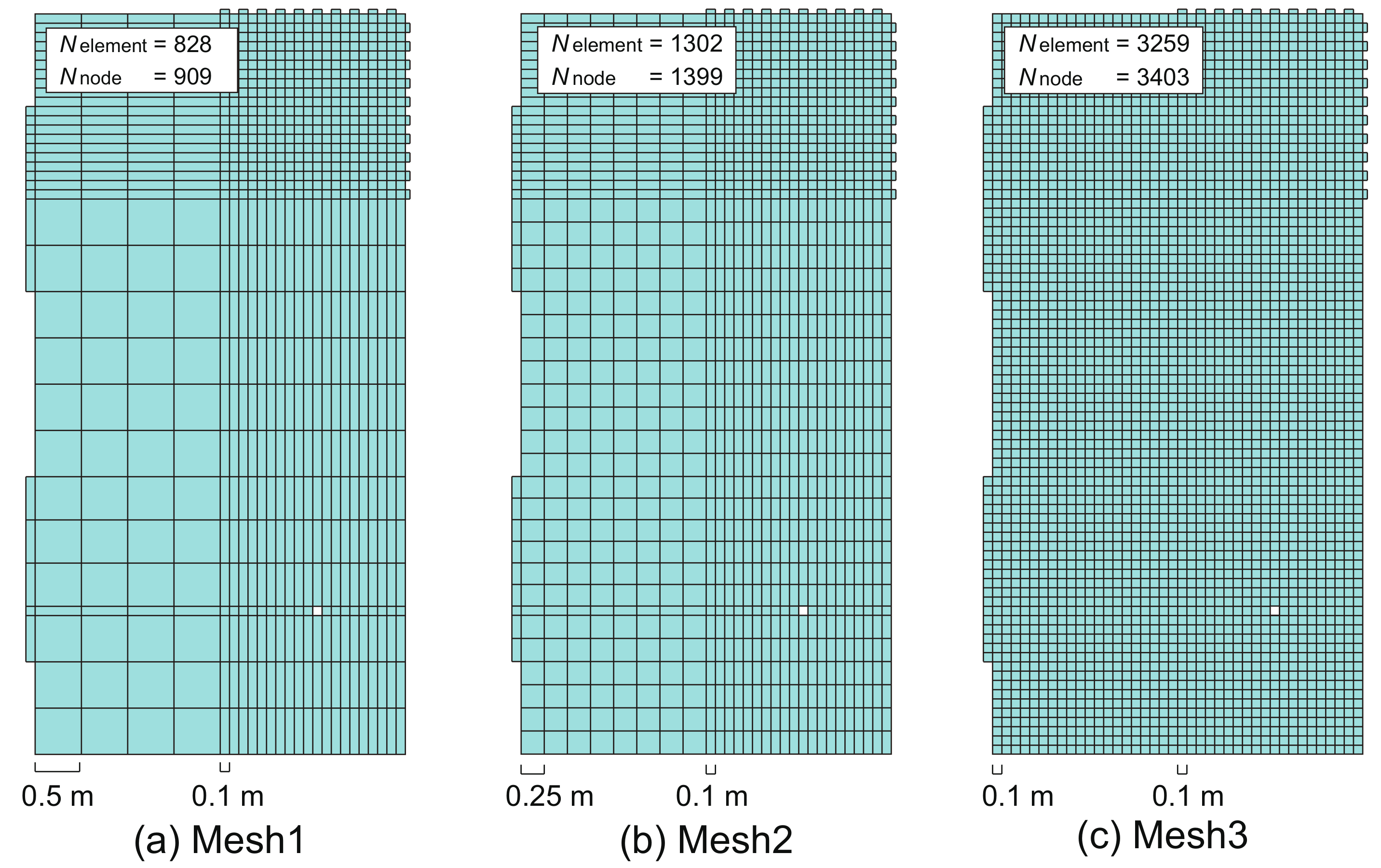
| Mesh 1 | Mesh 2 | Mesh 3 | Mesh 1 | Mesh 2 | Mesh 3 | |
| 828 | 1302 | 3259 | 808 | 1282 | 3239 | |
| 909 | 1399 | 3403 | 869 | 1359 | 3363 | |
| 0.1–0.5 m | 0.1–0.25 m | 0.1 m | 0.1–0.5 m | 0.1–0.25 m | 0.1 m | |
| 0.006–5.88 | 0.006–2.94 | 0.006–1.18 | 0.006–5.88 | 0.006–2.94 | 0.006–1.18 | |
| Model A | ||
|---|---|---|
| 20 Hz–2 kHz | 2–4 kHz | |
| 51,984 | 207,936 | |
| 209,008 | 833,888 | |
| h | 0.025 m | 0.0125 m |
| 0.001–0.15 | 0.074–0.15 | |
Publisher’s Note: MDPI stays neutral with regard to jurisdictional claims in published maps and institutional affiliations. |
© 2022 by the authors. Licensee MDPI, Basel, Switzerland. This article is an open access article distributed under the terms and conditions of the Creative Commons Attribution (CC BY) license (https://creativecommons.org/licenses/by/4.0/).
Share and Cite
Mukae, S.; Okuzono, T.; Sakagami, K. On the Robustness and Efficiency of the Plane-Wave-Enriched FEM with Variable q-Approach on the 2D Room Acoustics Problem. Acoustics 2022, 4, 53-73. https://doi.org/10.3390/acoustics4010004
Mukae S, Okuzono T, Sakagami K. On the Robustness and Efficiency of the Plane-Wave-Enriched FEM with Variable q-Approach on the 2D Room Acoustics Problem. Acoustics. 2022; 4(1):53-73. https://doi.org/10.3390/acoustics4010004
Chicago/Turabian StyleMukae, Shunichi, Takeshi Okuzono, and Kimihiro Sakagami. 2022. "On the Robustness and Efficiency of the Plane-Wave-Enriched FEM with Variable q-Approach on the 2D Room Acoustics Problem" Acoustics 4, no. 1: 53-73. https://doi.org/10.3390/acoustics4010004
APA StyleMukae, S., Okuzono, T., & Sakagami, K. (2022). On the Robustness and Efficiency of the Plane-Wave-Enriched FEM with Variable q-Approach on the 2D Room Acoustics Problem. Acoustics, 4(1), 53-73. https://doi.org/10.3390/acoustics4010004