Linear Iterative Procedure to Solve a Rayleigh–Plesset Equation

Abstract

A nonlinear Rayleigh–Plesset equation for describing the behavior of a gas bubble in an acoustic field written in terms of bubble-volume variation is solved through a linear iterative procedure. The model is validated, and its accuracy and fast convergence are shown through the analysis of several examples of different physical meanings. The simplicity and usefulness of the presented method here in relation to the direct resolution of the whole nonlinear system, which is also discussed, make the method very attractive to solving a problem. This iterative method allows us to solve only linear systems instead of the nonlinear differential problem. Moreover, the implementation of the iterative algorithm includes a tolerance-dependent stopping criterion that is also tested.

1. Introduction

Rayleigh–Plesset (RP) equations model the behavior of gas bubbles impinged by an acoustic wave under the consideration of some physical approximations [1,2]. Two frameworks exist in this context. On the one hand, the radius model uses time-dependent bubble radius $R\left(t\right)$ in the derivation of an ordinary differential equation. On the other hand, the volume model uses bubble volume variation $v\left(t\right)$ as a time-dependent variable for deriving an ordinary differential equation (RPv). In this work, we consider the latest. Such nonlinear differential model is of second-order. Two initial conditions on primary variable v and its first time derivative $v^{\prime }$ are required at the onset of the physical phenomenon ($t=0$). This model equation was derived in 1973 by Zabolotskaya et al. [3]. It was used in conjunction with the wave equation to analyze effects caused by a population of gas bubbles in a liquid, which parameter of nonlinearity increases by several orders of magnitude, on an ultrasonic field through the development of second-order perturbation methods [3,4] and numerical models [5,6,7,8].

The iterative procedure applied in this work to solve the RPv equation follows the iterative method developed for solving problems defined by nonlinear second-order ordinary differential equations [9]. This method relies on an iterative procedure that considers the differential equation at each iteration by assuming its nonlinear terms as known from the previous iteration, which leads to the expression of a modified reformulated linear problem at each iteration, so that only linear differential equations must be solved throughout the entire process (no nonlinear ordinary differential equations have to be explicitly solved). This latter point is an advantage regarding other techniques that need to solve nonlinear systems at each iteration step. When integrals at each iteration step can be analytically evaluated or by means of symbolic computations, it allows for the solution to be expressed in polynomial form. When these integrals cannot be analytically or symbolically solved (such as in this work, see Section 2), an alternative method consists of numerically calculating the integrals.

In this paper, we develop an iterative procedure to solve the initial-value Rayleigh–Plesset problem defined by the RPv equation to track in time the oscillations of a single bubble in an ultrasonic field. Section 2 describes the application of the technique. To this end, the system obtained at each iteration is numerically solved. Analysis of several physical examples and a comparison to the reference data are presented in Section 3, thus showing its fast convergence and accuracy. The simplicity and usefulness of the method are also discussed through these examples. A stopping criterion is also developed in the implemented algorithm. Lastly, Section 4 concludes this work.

2. Materials and Methods

We consider a tiny air bubble placed in liquid and impinged by an ultrasonic field. To describe the response of the bubble to the acoustic field, we work within the Rayleigh–Plesset framework. In this context, some approximations are applied to model the behavior of bubble oscillations, and several physical assumptions are made:

• bubble content is gas without vapor;
• the bubble is spherical (spherically symmetric pulsation);
• the gas contained in the bubble has adiabatic behavior;
• surface tension at the gas–liquid boundary is neglected;
• a quadratic Taylor expansion of the adiabatic gas law limits bubble oscillations to moderate values;
• the bubble does not itself radiate sound.

Moreover, in this work, we neglect buoyancy, Bjerknes, and viscous drag forces. The evolution with time t of the volume variation of the bubble $v\left(t\right)=V_b\left(t\right)-V_{b0}$, a smooth real-value function of t, where $V_b$ and $V_{b0}=4\pi R_{b0}^3/3$ are the current and initial volumes of the bubble, respectively, and $R_{b0}$ is the initial radius, is modeled by the Rayleigh–Plesset equation (RPv) [3,4],

$$v^{″}+\delta {\omega }_b{v}^{\prime }+{\omega }_b^{2}v-a{v}^2-b(2v{v}^{″}+{v^{\prime }}^2)=-\eta p,0<t<T,$$

(1)

in which $v^{\prime }$ and $v^{″}$ are the first- and second-order derivatives of $v\left(t\right)$, ${\omega }_b=\sqrt{3\gamma p_b/{\rho }_l{R}_{b0}^2}$ is the resonance frequency of the bubble, where ${\rho }_l$ is the density of the liquid at the equilibrium state, $\gamma$ is the specific heat ratio of the gas, $p_b={\rho }_b{c}_b^2/\gamma$ is its atmospheric pressure, ${\rho }_b$ and $c_b$ are the density and sound speed at the equilibrium state of the gas, and $\delta =4{\nu }_l/{\omega }_b{R}_{b0}^2$ is the viscous damping coefficient, for which ${\nu }_l$ is the kinematic viscosity of the liquid. $a=(\gamma +1){\omega }_b^2/2V_{b0}$ is the second-order nonlinear parameter due to the adiabatic law used to model the gas pressure inside the bubble. $b=1/6V_{b0}$ is the nonlinear coefficient associated to the bubble dynamics. The parameter $\eta =4\pi R_{b0}/{\rho }_l$ is a constant that affects the source term $p\left(t\right)$, which is the time-dependent acoustic pressure perturbation that impinges the bubble (a known source function). Several source functions are considered in Section 3. $t=T$ is the upper limit of the time interval. The derivation of this ordinary differential equation, Equation (1), can be found in [3,4].

The differential system is closed by imposing initial conditions expressing the rest of the bubble at the onset of the study (nonperturbation of the bubble at the start of the experiment),

$$v\left(0\right)=0,v^{\prime }\left(0\right)=0.$$

(2)

The iterative procedure relies on the resolution of several successive systems $D{S}_n$, which include the linear terms in the ordinary differential equation (linear operator L), the terms in the ordinary differential equation that do not depend on the dependent variable v (function g), and the initial conditions of the differential system (auxiliary operator A), through an $n-$ iterative process that starts at $n=0$ without considering nonlinear terms in the ordinary differential equation (nonlinear operator N), giving the solution $v_0\left(t\right)$, and follows for $n=1,\dots ,N$ by taking into account the nonlinear operator N evaluated at the preceding iteration, giving the solution $v_n\left(t\right)$:

$D{S}_0(n=0)$;

$$L\left(v_0\left(t\right)\right)+g\left(t\right)=0,A(v_0,v_0^{\prime })=[v_0\left(0\right)=0;v_0^{\prime }\left(0\right)=0],$$

(3)

$D{S}_n(n=1,\dots ,N)$;

$$L\left(v_n\left(t\right)\right)+g\left(t\right)+N\left(v_{n-1}\left(t\right)\right)=0,A(v_n,v_n^{\prime })=[v_n\left(0\right)=0;v_n^{\prime }\left(0\right)=0].$$

(4)

Its application to Equations (1) and (2) requires the definition of linear operator L (linear terms of the differential equation), nonlinear operator N (nonlinear terms), known function g (independent terms on v), and auxiliary operator A (initial conditions), respectively:

$$L\left(v\left(t\right)\right)=v^{″}+\delta {\omega }_b{v}^{\prime }+{\omega }_b^{2}v,$$

(5)

$$N\left(v\left(t\right)\right)=-a{v}^2-b(2v{v}^{″}+{v^{\prime }}^2),$$

(6)

$$g\left(t\right)=\eta p\left(t\right),$$

(7)

$$A(v,v^{\prime })=[v\left(0\right)=0;v^{\prime }\left(0\right)=0],$$

(8)

In this case, successive iterations are, for $D{S}_0$,

$$\left\{\begin{array}{l}L\left(v_0\left(t\right)\right)+g\left(t\right)=v_0^{″}+\delta {\omega }_b{v}_0^{\prime }+{\omega }_b^2{v}_0+\eta p=0,\\ A(v_0,v_0^{\prime })=[v_0\left(0\right)=0;v_0^{\prime }\left(0\right)=0],\end{array}\right.$$

(9)

and for $D{S}_n$,

$$\left\{\begin{array}{ll}L\left(v_n\left(t\right)\right)+g\left(t\right)+N\left(v_{n-1}\left(t\right)\right)& =v_n^{″}+\delta {\omega }_b{v}_n^{\prime }+{\omega }_b^2{v}_n+\eta p\\ & -a{v}_{n-1}^2-b(2v_{n-1}{v}_{n-1}^{″}+{v\prime }_{n-1}^2)=0,\\ A(v_n,v_n^{\prime })=[v_n\left(0\right)=0;v_n^{\prime }\left(0\right)& =0].\end{array}\right.$$

(10)

Each differential system obtained at each iteration n, Equations (9) and (10), is defined by a linear (in terms of $v_0$ and $v_n$, respectively) inhomogeneous second-order ordinary differential equation of time-dependent variable $v_0$ and $v_n$, respectively, and Cauchy conditions. Finding the analytical solution of Equation (10) is not straightforward. Symbolic calculus was used to obtain this solution at each iteration of the progression, but it failed in giving $v_n$ from $n=2$ due to the complexity of the second-hand side of Equation (10).

Thus, we chose to apply a numerical scheme at each iteration n, namely, the second-order explicit vector Euler approximation method [10], which is more efficient than solving the whole problem directly, Equations (1) and (2), numerically. A fourth-order vector Runge–Kutta algorithm was also developed, but the obtained results in the following section were not affected by the choice of numerical method. To this purpose, we reduce $D{S}_0$ and $D{S}_n$ to a nonlinear first-order system of two coupled ordinary differential equations by setting the new variable $v^{\prime }\left(t\right)=V\left(t\right)$, which yields

$$\left\{\begin{array}{cc}\hfill v_0^{\prime }\left(t\right)& =V_0\left(t\right)=f_{v0}(t,v_0,V_0),\hfill \\ \hfill v_0\left(0\right)& =0,\hfill \\ \hfill V_0^{\prime }\left(t\right)& =-\delta {\omega }_b{V}_0\left(t\right)-{\omega }_b^2{v}_0\left(t\right)-\eta p\left(t\right)=f_{V0}(t,v_0,V_0),\hfill \\ \hfill V_0\left(0\right)& =0,\hfill \end{array}\right.$$

(11)

$$\left\{\begin{array}{cc}\hfill v_n^{\prime }\left(t\right)& =V_n\left(t\right)=f_{vn}(t,v_n,V_n),\hfill \\ \hfill v_n\left(0\right)& =0,\hfill \\ \hfill V_n^{\prime }\left(t\right)& =-\delta {\omega }_b{V}_n\left(t\right)-{\omega }_b^2{v}_n\left(t\right)-\eta p\left(t\right)\hfill \\ \hfill & +a{v}_{n-1}^2\left(t\right)+b(2v_{n-1}\left(t\right)V_{n-1}^{\prime }\left(t\right)+V_{n-1}^2\left(t\right))=f_{Vn}(t,v_n,V_n),\hfill \\ \hfill V_n\left(0\right)& =0.\hfill \end{array}\right.$$

(12)

These differential systems are written in the following vector form, after defining ${\mathit{V}}_n\left(t\right)={(v_n\left(t\right),V_n\left(t\right))}^t$, ${\mathit{F}}_n(t,{\mathit{V}}_n)={(f_{vn}(t,v_n,V_n),f_{Vn}(t,v_n,V_n))}^t$, $\mathbf{0}={(0,0)}^t$,

$$\left\{\begin{array}{cc}\hfill {\mathit{V}}_0^{\prime }\left(t\right)& ={\mathit{F}}_0(t,{\mathit{V}}_0),\hfill \\ \hfill {\mathit{V}}_0\left(0\right)& =\mathbf{0},\hfill \end{array}\right.$$

(13)

$$\left\{\begin{array}{cc}\hfill {\mathit{V}}_n^{\prime }\left(t\right)& ={\mathit{F}}_n(t,{\mathit{V}}_n),\hfill \\ \hfill {\mathit{V}}_n\left(0\right)& =\mathbf{0}.\hfill \end{array}\right.$$

(14)

The application of the above-mentioned numerical algorithm to Equations (13) and (14) requires the discretization of the continuous time domain by means of the time discretization step h, giving the set $\left\{t_i\right.{\}}_{i=1}^I$, where $I=(T-0)/h+1$. The approximate solution of Systems (13) and (14) is sought at all points $t_i$ of that set (subindex i indicates the approximate value of the corresponding variable at point $t_i$). This process leads to the following formulation:

$$\left\{\begin{array}{cc}\hfill {\mathit{V}}_{0,i+1}& ={\mathit{V}}_{0,i}+h{\mathit{F}}_0(t_i,{\mathit{V}}_{0,i}),1\le i\le I-1,\hfill \\ \hfill {\mathit{V}}_{0,1}& =\mathbf{0},\hfill \end{array}\right.$$

(15)

$$\left\{\begin{array}{cc}\hfill {\mathit{V}}_{n,i+1}& ={\mathit{V}}_{n,i}+h{\mathit{F}}_n(t_i,{\mathit{V}}_{n,i}),1\le i\le I-1,\hfill \\ \hfill {\mathit{V}}_{n,1}& =\mathbf{0}.\hfill \end{array}\right.$$

(16)

The derivative $V_{n-1,i}^{\prime }$ in Equation (16), $V_{0,i}^{\prime }$ when $n=1$, is evaluated at each point $t_i$ through a first-order finite-difference formula [10].

Since no exact solution of our differential problem is known, we evaluate the error produced during the iterative process through the discrete $L_2$-norm of the difference between two consecutive approximate solutions, ${\mathit{V}}_n(i,1)$ and ${\mathit{V}}_{n-1}(i,1)$ on the one hand, i.e., $v_{n,i}$ and $v_{n-1,i}$, and between ${\mathit{V}}_n(i,2)$ and ${\mathit{V}}_{n-1}(i,2)$ on the other hand, i.e., $v_{n,i}^{\prime }$ and $v_{n-1,i}^{\prime }$, at each point i of the discretization set $t_i$ for $i=1,\dots ,I$, and for all values $n=1,\dots ,N$, which is the ${\mathit{E}}_{{\mathit{V}}_n}^{L_2}$-vector of components:

$$\begin{array}{c}\hfill E_{v_n}^{L_2}=\sqrt{\sum _{i=1}^I{(v_{n,i}-v_{n-1,i})}^2},\\ \hfill E_{v_n^{\prime }}^{L_2}=\sqrt{\sum _{i=1}^I{(v_{n,i}^{\prime }-v_{n-1,i}^{\prime })}^2}.\end{array}$$

(17)

The objective of this paper is to propose a very useful tool for solving the problem described above. In this context, a stopping criterion is set from the value of the tolerance, $ϵ$, as follows. Iterations stop as soon as both inequalities stand:

$$\begin{array}{c}\hfill E_{v_n}^{L_2}\le ϵ,E_{v_n^{\prime }}^{L_2}\le ϵ,\end{array}$$

(18)

for which tolerance could be defined as, for instance, $ϵ=v_{b0}\times {10}^{-10}$. An example of using the stopping criterion is given in Section 3.

The ad hoc implementation of the scheme is performed in a MATLAB${}^{\circledR }$ R2017a environment. The schematic workflow for the successive steps of the entire algorithm is represented in Figure 1. CPU times required to obtain the solution of the bubble problems from the resolution process, indicated by $t_{cpu}$ in the following paragraphs, are obtained by running the code on a 128 GB RAM computer with a 64 bit Windows 10 operative system working with an Intel${}^{\circledR }$ Core™ i7-6800 K CPU @ 3.40 GHz.

3. Results and Discussion

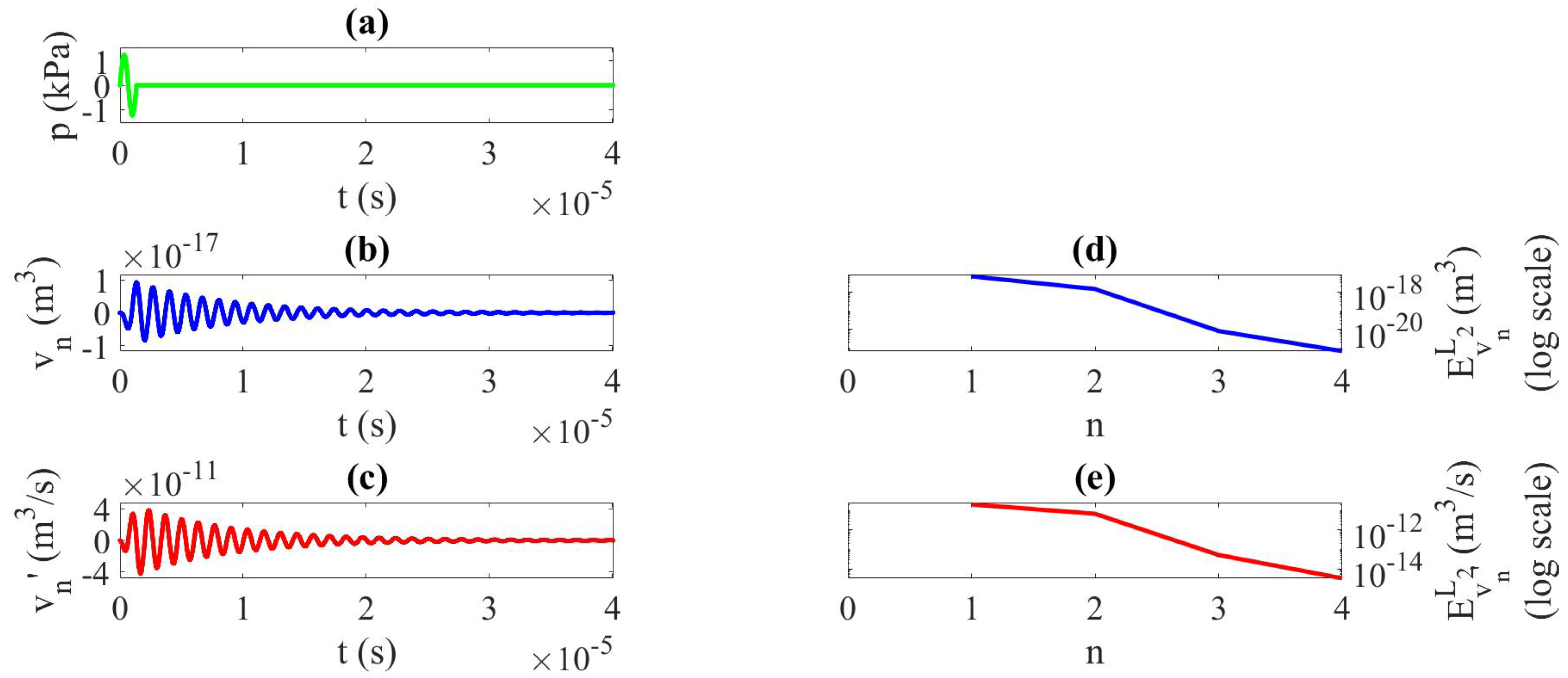
In this section, the method developed in Section 2 is applied to solve the following physical problem: in water (${\rho }_l=1000$ kg/m${}^3$, ${\nu }_l=1.43\times {10}^{-6}$ m${}^2$/s), an air bubble of initial radius $R_{b0}=4.5\mathsf{\mu }$m (${\rho }_b=1.29$ kg/m${}^3$, $c_b=340$ m/s, $\gamma =1.4$, $p_b=0.11$ MPa, ${\omega }_b=4.7$ MHz) is impinged by a continuous (monochromatic) sine ultrasonic wave, $p\left(t\right)=p_{0}sin\left(\omega t\right)$, of frequency $f=\omega /2\pi =f_b={\omega }_b/2\pi =748.07$ kHz and high finite amplitude $p_0=1.25$ kPa, studied during $T=30/f$ (see Figure 2a), and for the number of iterations $N=14$, Case 1. $\delta =0.06$, $\eta =5.66\times {10}^{-8}$ m${}^4$/kg, and time step $h=1\times {10}^{-9}$ s are used in the entire section. $t_{cpu}=406$ s in Case 1. Figure 2 represents (a) the pressure source signal; the solution at the last iteration $n=N$, i.e., (b) the bubble volume variation $v_N$ and (c) the speed of bubble volume variation $v_N^{\prime }$. The $L_2$-norm error at each iteration of the calculation is shown in Figure 2d,e, respectively, for $v_n$ and $v_n^{\prime }$. The convergence of the method is fast (Figure 2d,e). Figure 3 displays the comparison of the obtained results here to the obtained data by a simulation carried out with the Snow-Bl code considering one single bubble with the same parameters [5]. This code relies on the approximation of the solution of Equation (1), coupled to the linear wave equation, by finite-difference approximations. It can track both pressure and bubble oscillation fields in time. The concordance of both bubble-volume variation results validates the method developed in this paper. The CPU time needed by the Snow-Bl code is 4893 s, which is 12 times the time required here.

Figure 4 shows the corresponding results for the infinitesimal source amplitude $p_0=1\times {10}^{-3}$ Pa, Case $1^{\prime }$, which implies a linear behavior of the bubble response since the nonlinear parameters a and b are multiplied by very small values. Convergence is thus immediate, after one iteration. Figure 5 shows the corresponding results for the same finite source amplitude as that in Case 1, $p_0=1.25$ kPa, but after setting nonlinear parameters a and b to zero, Case $1^{″}$. This imposition implies a linear response of the bubble even at this high source amplitude since ordinary differential Equation (1) is linear. The solution is reached at the first calculation for $v_0$ and $v_0^{\prime }$, and no iterations are needed. The comparison of the solution, especially v, for Cases $1^{\prime }$ and $1^{″}$ reveals that both curves are identical (proportionally to their amplitude) in Figure 4 and Figure 5, i.e., the result is similar in both cases. However, in Figure 2 for Case 1, the nonlinearity due to finite amplitude and nonlinear parameters a and b affects the system and modifies the solution iteration by iteration, which leads to a different signal, showing distortion and a slight nonsymmetrical response between positive and negative volume variations around axis $v=0$.

To illustrate the possibilities and usefulness of the method implemented in this paper, we consider two other forcing terms in Equation (1): a one-cycle burst ultrasonic signal of frequency $f=200$ kHz and high finite amplitude $p_0=1.25$ kPa, studied during $T=30/f$ (see Figure 6a), and for the number of iterations $N=4$, Case 2; an ultrasonic pulse of frequency $f=200$ kHz and finite amplitude $p_0=1$ Pa, studied during $T=100/f$ (see Figure 7a), and for a number of iterations $N=4$, Case 3. $t_{cpu}=40$ s for Case 2, and $t_{cpu}=542$ s for Case 3. For each case, we represent the response of the system by displaying (a) the pressure source signal, (b) the bubble-volume variation $v_N$, (c) the speed of bubble-volume variation $v_N^{\prime }$ at the last iteration $n=N$, and the $L_2$-norm at each iteration of the calculation in Figure 6d,e and Figure 7d,e respectively, for $v_n$ and $v_n^{\prime }$. These diagrams correspond to Figure 6 for Case 2 and Figure 7 for Case 3, respectively. The physically coherent response of the system (Figure 6b,c and Figure 7b,c) is obtained after very few iterations (Figure 6d,e and Figure 7d,e), which illustrates the good behavior of the method developed in this work.

For Case 1, we test the stopping criterion given by (18) with $ϵ=v_{b0}\times {10}^{-1}$, $ϵ=v_{b0}\times {10}^{-10}$, and $ϵ=v_{b0}\times {10}^{-20}$. Results are shown in Figure 8. $N=7$ with $t_{cpu}=105$ s, $N=26$ with $t_{cpu}=1424$ s, and $N=63$ with $t_{cpu}=8450$ s are respectively required for satisfying the tolerance. Figure 8c shows an extremely exigent case since it takes many iterations to slightly decrease error and improve results $v_n$ and $v_n^{\prime }$.

In the three cases presented in this section, even though the parameters of the problem set two very high nonlinear coefficients, $a=6.95\times {10}^{+28}$ Hz${}^2$/m${}^3$ and $b=4.37\times {10}^{+14}$/m${}^3$, the convergence of the presented method is fast, indicating the good behavior of the method. Regarding the benefits obtained here to solve the RPv in relation to other potential or existing resolution methods, the following arguments are given. (i) First, the direct treatment of the complete nonlinear differential system by reducing its order to 1 would end up requiring a numerical resolution (vector Newton–Raphson or similar algorithm) of a nonlinear coupled system of two discretized equations (for which the nonlinear operator N would depend on the unknown variable $N\left(v_n\right)$ instead of the known solution at the previous iteration $N\left(v_{n-1}\right)$ in Equation (10) of the current procedure) at each step of the numerical process (vector Runge–Kutta or vector explicit Euler method), of which the time cost is elevated, and accuracy depends on the choice of the required vector estimation to start the system resolution. A clear advantage of the presented model is that it does not need such intermediate solution to nonlinear systems since the nonlinear terms used are known from the previous iteration. (ii) On the other hand, the direct treatment of the complete nonlinear differential system of second order, Equations (1) and (2), is much likely to be more delicate and time-consuming. The direct substitution of derivatives by finite-difference formulas in Equations (1) and (2) would lead to an implicit scheme requiring the resolution of a nonlinear system of equations at each time step of the process, which is usually highly time-consuming. The treatment of differential system Equations (1) and (2) by finite-volume time approximations would end up to a quite similar resolution of nonlinear systems of equations at the time steps. The use of finite-element approximations through the application of a variational formulation to obtain a weighted-integral form equivalent to Equations (1) and (2) would also require the solution of a nonlinear system of equations at each step of the time discretization process (finite differences). Thus, the simplicity of the procedure presented in this paper makes it very useful and attractive.

4. Conclusions

A nonlinear Rayleigh–Plesset equation written in the bubble variation volume framework was solved through a linear iterative procedure. The presented results showed fast convergence and accuracy of the technique developed in this paper. The simplicity and usefulness of the method presented here in relation to the direct resolution of the whole nonlinear system was also discussed. This iterative method allowed us to solve only linear systems instead of a nonlinear differential problem. Moreover, the implementation of the iterative algorithm includes a tolerance-dependent stopping criterion that was also tested.