Article

Experimental and Analytical Investigation of the Tonal Trailing-Edge Noise Radiated by Low Reynolds Number Aerofoils

1
Laboratoire de Mécanique des Fluides et d’Acoustique, Université de Lyon, École Centrale de Lyon, F-69134 Écully, France
2
Département de génie mécanique, Université de Sherbrooke, Sherbrooke, QC J1K2R1, Canada
3
Aerospace Engineering Department, Embry-Riddle Aeronautical University, Daytona Beach, FL 32114-3900, USA
*
Author to whom correspondence should be addressed.
These authors contributed equally to this work.
Acoustics 2020, 2(2), 293-329; https://doi.org/10.3390/acoustics2020018
Submission received: 18 March 2020 / Revised: 1 May 2020 / Accepted: 8 May 2020 / Published: 14 May 2020

Abstract

:
An experimental and analytical study of the tonal trailing-edge noise of a symmetric NACA-0012 aerofoil and of a cambered SD7003 aerofoil has been achieved. It provides a complete experimental database for both aerofoils and improves the understanding of the underlying mechanisms. The analysis stresses the high sensitivity of the tonal noise phenomenon to the flow velocity and the angle of attack. Several regimes of the noise emission are observed depending on the aforementioned parameters. The contributions of the pressure and the suction sides are found to vary with the flow parameters too. A special attention has been paid to the role of the separation bubble in the tonal noise generation. Hot-wire measurements and flow visualization prove that the separation bubble is a necessary condition for the tonal noise production. Moreover, the bubble must be located close enough to the trailing edge. Several tests with small-scale upstream turbulence confirm the existence of the feedback loop. Analytical predictions with a classical trailing-edge noise model show a good agreement with the experimental data; they confirm the cause-to-effect relationship between the wall-pressure fluctuations and the radiated sound. Finally, previously reported works on fans and propellers are shortly re-addressed to show that the tonal noise associated with laminar-boundary-layer instabilities can take place in rotating blade technology.

1. Introduction

Tonal trailing-edge noise refers to the loud, annoying whistling sometimes produced lifting surfaces at low Reynolds numbers and moderate angles of attack in a clean flow. It is heard not only in laboratory experiments involving aerofoils in controlled flow conditions, but also in rotating-blade engineering applications. Most often, true tones are identified in the first case, and a narrow-band spectral peak is emitted in the second case. This suggests that a well-defined tonal character a priori requires spanwise-homogeneous conditions such as those ensured by the wind-tunnel mounting of rectangular aerofoils. Typically, glider wings emit tonal trailing-edge noise during some operations because the incident flow normal to the wing span is close to these conditions. In contrast, rotating-blade technologies make a more or less broadband or narrow-band signature instead of discrete frequencies because the flow conditions vary along the blade span. In fact, different acoustic signatures can be produced depending on blade design and on the portion of span actually involved in the generation of noise. For instance, a peak at much higher frequencies than the rotational noise has been reported for a low-speed fan by Longhouse [1], whereas a signature very similar to those of rectangular isolated aerofoils with multiple tones has been observed during the wind-tunnel testing of model propellers by Grosche and Stiewitt [2]. Both examples are discussed later on in the paper. Yet, for simplicity the wording ‘tonal noise’ is used in all cases throughout the paper.
The common necessary feature for the generation of tonal noise is the existence of an unstable, laminar/transitional boundary layer all over the aerofoil, or at least on one side. Indeed, forcing the transition to turbulence before the trailing edge by appropriate tripping suppresses the tones and produces low-level broadband trailing-edge noise. In that sense, tonal noise is characteristic of low Reynolds numbers. Instabilities in the boundary layers are a key factor for the emission of the sound by interaction with the trailing edge. For this reason the mechanism is referred to as Laminar-Boundary-Layer (LBL) wave radiation in this work, to be related to the LBL vortex-shedding noise according to the classification by Brooks et al. [3]. The same mechanism is called vortex shedding by Longhouse [1]. It has been thoroughly investigated over the last 50 years but some details of the underlying physics still remain points of controversy. Apart from its fundamental interest LBL-wave radiation is a matter of concern for all aerofoils and blades used in unmanned air vehicles (UAV) and micro air vehicles (MAV) that operate at low Reynolds numbers and that are promised to an intensive use in the near future.
After Fink [4] and other works reviewed for instance by Longhouse [1], Paterson et al. [
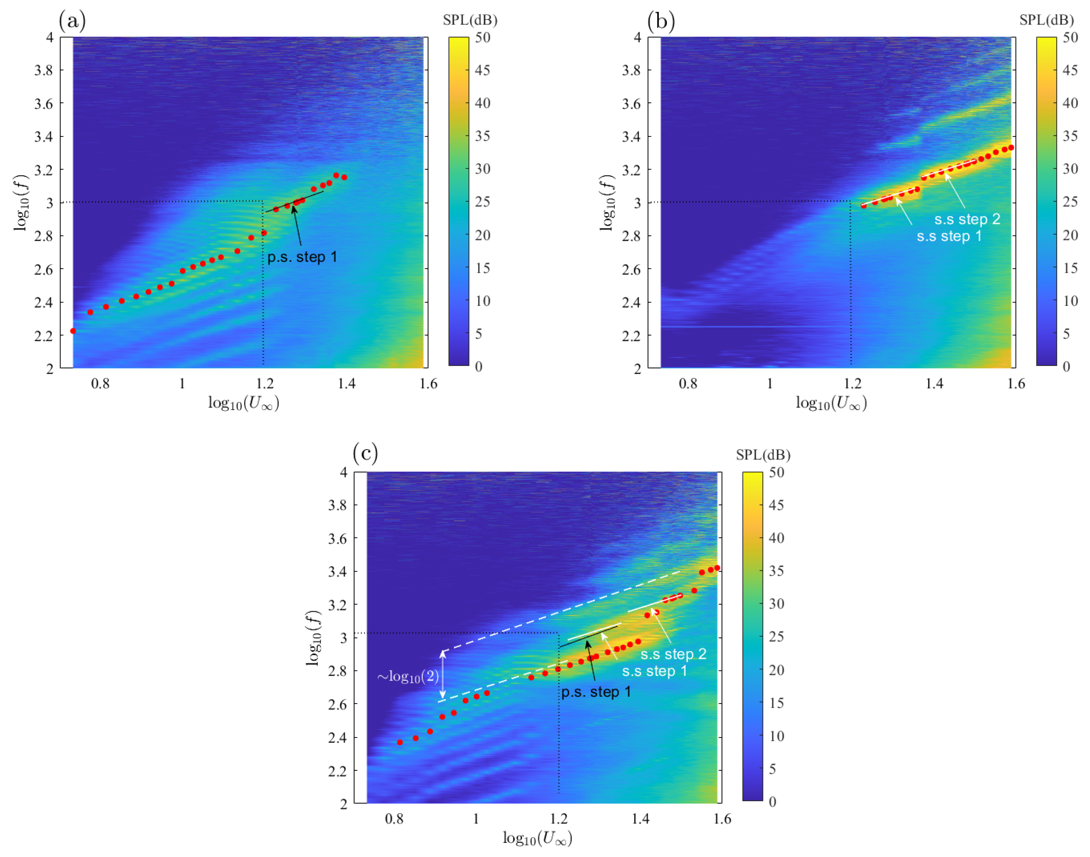
5] published a detailed study of the far-field tonal noise of the NACA-0012 aerofoil in an open-jet wind tunnel. A so-called ladder-type structure was observed when the frequency of the dominant tone was plotted as an increasing function of flow velocity. The global slope was found to approximately correspond to the law f U 1.5 , where f was the frequency and U the incident flow speed, whereas the steps followed parallel lines scaling with a law close to f U 0.8 . Tam [6] conjectured that an acoustic feedback loop took place between some source point in the wake and the trailing edge to explain the ladder-type structure. Longhouse later argued that the feedback rather took place between the trailing edge and an upstream point [1]. He suggested that Tollmien–Schlichting (TS) waves generated at some initial point in the suction-side boundary layer of a cambered aerofoil were convected downstream toward the trailing edge where they scattered as sound. The acoustic waves propagating upstream were able to amplify the instabilities at some frequencies for which a favourable phase condition was fulfilled, yielding the emergence of discrete tones in the sound spectrum. The same interpretation was refined by Arbey and Bataille [7] who stressed that the noise combined two components, namely a hump-like signature associated with the natural frequency range of the boundary-layer instabilities and discrete tones reinforced by the acoustic feedback loop identified by Longhouse. When simulating the NACA-0012 aerofoil at non-zero angle of attack, Desquesnes et al. pointed out that a primary feedback loop was set on the pressure side [8]. They also assumed the existence of a second feedback loop on the suction side. The double feedback mechanism on a NACA-0012 aerofoil at non-zero angle of attack was also been assumed by Arcondoulis [9] to explain multiple observed tones with high intensity.
Yet, this feature is not essential because only one laminar boundary layer, the opposite one being turbulent, is enough to ensure the emission of tones. It can therefore be guessed that several regimes of feedback take place depending on the flow conditions [10]. Chong and Joseph [11] inspected the relationships between the tones and confirmed that the lag between the frequency of maximum amplification for the instabilities and the multiple discrete tones caused the jumps of the dominant tonal frequency.
Some apparent contradiction was raised as the ladder-type structure was not found during measurements performed in a closed-section wind tunnel by Nash et al. [12,13]. The authors only observed a regular, monotonic frequency increase with flow speed. They suspected that previous studies in which the ladder-type structure was found were influenced by installation effects. Tests repeated in various open-jet installations including setups with narrow supports indicate that this should not be the case [14]. Later, Tam and Ju [15] showed on the basis of two-dimensional Direct Numerical Simulations (DNS) that only one tone was produced by the aerofoil and confirmed the assumption of Nash et al. [12]. Yet, in the considered range of transitional Reynolds number based on the chord length R e c between 2 and 5 × 10 5 , the 2D simulation might not yield a realistic turbulent flow. Some contributors also tried to bring out necessary and sufficient conditions for the effective emission of tones. Lowson et al. [16] concluded that coherent instabilities in a laminar boundary layer, on the one hand, and the formation of a separation bubble, on the other hand, are not sufficient conditions [12] if not associated. Other studies [17,18] evidenced that separation bubbles are involved in high-level tonal noise generation. Moreover, the location of the separation bubble strongly depends on the Reynolds number and on the angle of attack. Typically, this allows for suction-side dominated and pressure-side dominated regimes of tonal noise emission for the NACA-0012 aerofoil at low Reynolds numbers and at high Reynolds numbers, respectively. Acoustic measurements and particle image velocimetry (PIV) reported by Pröbsting et al. [18,19] indicate that the separation areas act as an amplifier for the instability waves. The authors also confirmed a ladder-type structure compatible with the aforementioned power laws identified by Paterson et al. [5]. Furthermore, a time-resolved analysis showed that the tone frequencies were associated with vortical patterns at the trailing edge. Gerakopulos and Yarusevych [20] used time-resolved wall-pressure measurements and hot-wire anemometry to investigate the separation bubbles on a NACA-0018 aerofoil. They observed a strong correlation between velocity fluctuations in the separated shear layer and wall-pressure fluctuations, and deduced values of the convection speed of the instabilities from measurements on pairs of wall microphones. A similar investigation will be detailed later on.
Except for the rotating-blade applications, most aforementioned isolated-aerofoil studies focused on the NACA-0012 aerofoil, which provides a reference configuration for comparing works by various teams. Padois et al. [10,21] also investigated another aerofoil geometry of engineering interest, namely a Controlled-Diffusion (CD) aerofoil used for low-speed fans and turboengine-compressor blades. They observed the same tonal-noise mechanisms with similar characteristics. In their anechoic wind tunnel with low turbulence intensity (less than 4%), they also detected both stationary tones and intermittent ones depending on the Reynolds number R e c and the angle of attack. A Lattice-Boltzmann (LBM) DNS of the CD aerofoil by Sanjosé et al. [22] for an observed intermittent noise regime ( 5 geometric angle of attack) led to the identification of two states of quiet and intense events yielding the intermittent tone. The state switched in time depending on whether or not the laminar separation bubble was shedding weak or strong vortices. The vortices were formed from strong Kelvin–Helmholtz instabilities, which broke down near the trailing edge and induced transition to turbulence. This has been later confirmed by tomographic particle image velocimetry [23]. The synthesis of aforementioned observations makes the conjunction of a separation bubble and of large coherent structures a necessary condition to produce a significant tonal trailing-edge noise.
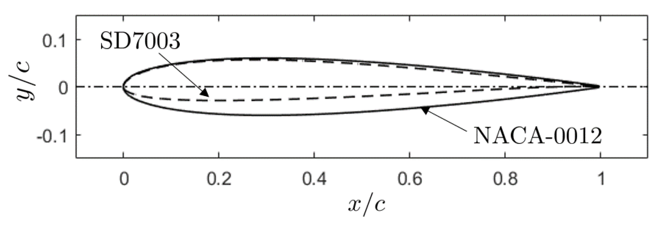
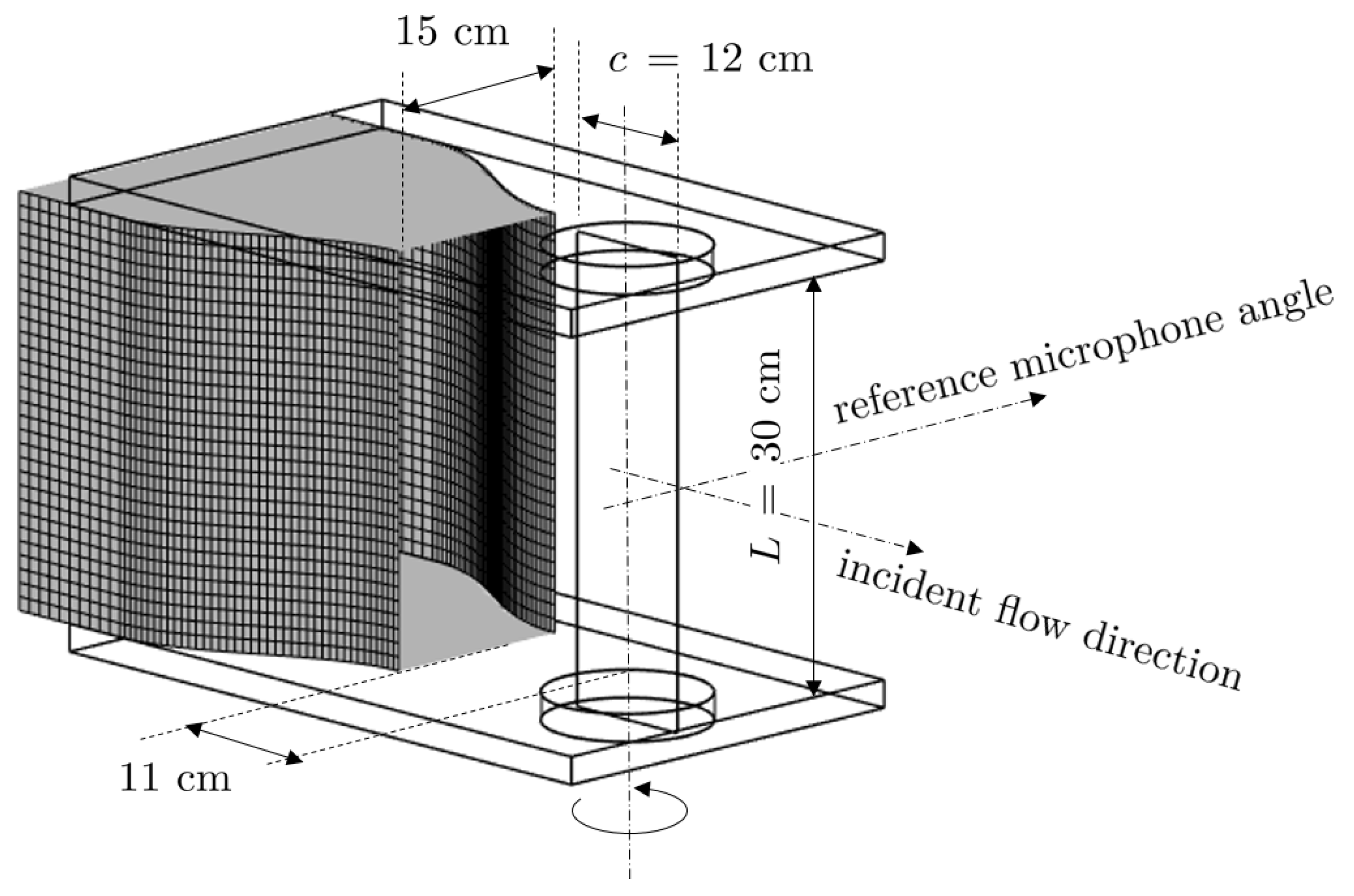
The present contribution is part of a collaborative research between Embry-Riddle Aeronautical University (ERAU) and Ecole Centrale de Lyon (ECL). It is aimed at completing the knowledge about tonal trailing-edge noise with experimental, analytical, and numerical investigations. The experimental study and the analytical modeling have been carried out at ECL [24,25] and the numerical simulations performed at ERAU [26,27,28]. Two aerofoils have been selected, namely the symmetric NACA-0012 aerofoil and a slightly cambered SD7003 aerofoil. The former is again taken as a well documented reference aerofoil, which allows comparing with previously reported studies. The latter is widely used in MAV and UAV and is also considered as a way of addressing the effect of aerofoil design on the noise emission.
The article presents key results of the extended experimental work achieved during the project, not exhaustively detailed for the sake of conciseness. Analytical predictions of some aspects of the mechanism are also used to discuss cause-to-effect relationships. The experiment is mainly aimed at confirming or refuting controversial points, such as:
  • the possible reason of discrepancies in experimental and numerical studies,
  • the role of the separation bubble in tonal noise generation,
  • the experimental setup issues,
and at providing a complete database for the validation of the numerical simulations by ERAU. The database includes the measurements of both aerodynamic and acoustic quantities, such as far-field acoustic pressure, wall-pressure statistics, mean-pressure coefficient, mean and fluctuating velocities and flow visualization. The time-frequency and bicoherence analyses have also been used as in [10]. Bicoherence is not discussed here because it could not help interpreting the mechanism, apart from confirming that the amplification of tones involves a significant nonlinearity. The experimental setup, aerofoil instrumentation and methodology are first described in Section 2. The main results and their interpretation are presented in Section 3. The noise emission regimes and the role of the separation bubble are highlighted during the discussion. The detailed analysis of the wall-pressure measurements with cross-spectral coherence and phase is presented to distinguish the aerodynamic and acoustic nature of recorded signals. The additional Section 4 is dedicated to the analysis of several experiments performed on low-speed fans and propellers. It proves that the laminar-boundary-layer instabilities are also observed in rotating machines. Finally Section 5 is dedicated to the analytical modeling of both near-field and far-field pressures associated with amplified tones.

2. Experimental Set-Up and Instrumentation

2.1. Aerofoil Installation

A symmetric NACA-0012 aerofoil and a cambered SD7003 aerofoil, the cross-sections of which are shown in Figure 1, have been selected for the present study. Both are made of aluminum, and have the same chord and wetted span of 12 and 30 cm, respectively. The measurements have been performed in an anechoic open-jet wind tunnel at ECL. A sketch of the experimental setup is shown in Figure 2. The nozzle outlet section has a height of 30 cm and a width of 15 cm. It delivers a uniform flow with a residual turbulence intensity below 0.8 % . The effect of this parameter will be discussed in Section 3.5.
The leading edge of the tested aerofoil is located 11 cm downstream of the nozzle exit, so that the aerofoil is embedded in the potential core of the jet. The flow velocity U ranges from 5 to 40 m/s. The associated chord-based Reynolds number and Mach number range from R e = 0.4 × 10 5 to 3.2 × 10 5 and from M = 0.015 to 0.12 , respectively. The aerofoil is mounted vertically, its ends fixed between two disks inserted in horizontal end-plates, which allows varying the geometrical angle of attack α between the aerofoil chord line and the direction of the incident flow. For the present investigation this angle has been typically varied from 15 to 15 with an uncertainty of ± 0.5 . The extreme angles are not considered.
The flow width to chord-length ratio is only 1.25, therefore the nozzle jet is substantially deviated by the equivalent lateral momentum injection at non-zero angle of attack. This reduces the effective loading with respect to what would be achieved in an infinite fluid. For a relevant investigation of trailing-edge noise sources the actual loading is a key parameter, because it conditions the transition in the boundary layers. Though an aerodynamic balance could be used to characterize it, developing boundary layers and associated trailing-edge noise are more precisely a matter of mean static-pressure distribution. The latter provides more information than the integrated lift. This distribution has been measured with a set of probes described later on. In principle, the mean pressure coefficient must be the same for the geometrical angle of attack on the experimental setup and the effective angle of attack in an infinite stream, so that the measurement can be considered as representative of the reference. When installation effects are moderate and for some aerofoil shapes, the desired effective angle of attack α * can be obtained by adjusting the geometrical angle α with a reasonably representative mean pressure coefficient. In the case of the NACA-0012 aerofoil such a correspondence has been established from Brook’s formula [3] with α / α * = 2.86 . However, for non-symmetric aerofoils and quite small flow-width to chord-length ratios, the reference pressure distribution may be impossible to reproduce in the wind-tunnel experiment, as pointed out by Moreau et al. [29] for a CD (Controlled-Diffusion) aerofoil. Nevertheless as long as the mean pressure coefficient is at least reasonably reproduced in the aft part of the aerofoil, the trailing-edge noise sources are comparable. For these reasons, the mean measured pressure coefficient for the SD7003 aerofoil has been compared with that predicted by two-dimensional Reynolds-Averaged Navier–Stokes (RANS) numerical simulations [25], following the methodology proposed in [29]. In particular the computational domain includes the nozzle.
The RANS simulations, not detailed here, showed that the geometrical angles α = 2 , 5 , 7 of the SD7003 aerofoil correspond to the effective angles α * = 0 , 1 , 2 , respectively.
The far-field pressure was measured by a Bruel and Kjaer 1 / 2 type 2671 microphone at the distance of 1.5 m for the NACA-0012 aerofoil and at 2.2 m for the SD7003 aerofoil at 90 with respect to the oncoming flow direction.
Another issue with the limited width of the nozzle jet is the possible contamination of the local flow over the aerofoil by the oscillations of the developing free shear-layers of the jet, especially at low frequencies. A preliminary test has thus been performed with and without a thin additional splitter-plate of 3 cm chord and 30 cm span placed parallel to the aerofoil at the border of the shear layer, close to the streamwise location of the aerofoil leading edge. The power spectral densities (PSD) of the far-field sound pressure measured at 90 are reported in Figure 3a,b for two flow speeds. Without the splitter-plate, the spectrum exhibits the hump and tones attributed to the typical trailing-edge noise of transitional aerofoils. As the splitter-plate is added, this signature is not significantly modified, except for a different amplitude of some of the tones, and an additional broad hump is evidenced at substantially lower frequencies. As an additional source of turbulence-impingement broadband noise, the splitter-plate gives information on the frequency content of the shear-layer oscillations. This test indicates that the frequency ranges of aerofoil and splitter-plate contributions are well separate. It also confirms that the oscillations of the wind-tunnel jet do not disturb directly the developing laminar instabilities of interest. It is also worth noting that the background noise, defined as the noise measured when suppressed the aerofoil, has been removed by simple subtraction of spectra [30,31]. Moreover, the frequency range below 100-200 Hz is contaminated by installation effects such as jet noise that make the true sources of background noise differ with and without the aerofoil installed. This is not a limitation in view of the much higher frequency range of the investigated tonal noise.
Complementary tests not reported in this paper have been performed with very narrow symmetric end-plates in order to minimize the possible confinement of acoustic waves (see also Golubev et al. [14]). This did not produce significant changes in the measured sound spectra and proved that, as long as the microphone is placed in the far field and in the mid-span plane, the measurements are free of spurious sound scattering by the end-plates. This is consistent with the scattering study performed by Moreau et al. [32].
Investigations reported in the literature stress the importance of the laminar and transitional character of the boundary layers on trailing-edge noise. Therefore, several configurations with tripping devices added on one side or the other, as well as on both sides, have been tested. The tripping device is a strip of medical adhesive plaster of 2.5 cm width located around the expected area of maximum local velocity. Typically, it was centred at a distance of 3 cm from the leading edge for the NACA-0012 aerofoil. The tripping forces transition of the laminar boundary layer to turbulence and deactivates the generation of tonal noise. The influence of a fine-scale homogeneous upstream turbulence has also been studied by inserting a turbulence grid before the nozzle contraction (see Figure 2). The grid has a square mesh with a side of 1 cm made of metal wires of 1.5 mm diameter and the contraction ratio is 2-to-1 in only the horizontal direction.

2.2. Aerofoil Instrumentation and Methodology

2.2.1. Remote-Microphone Probes

For wall-pressure measurements, each mock-up is instrumented with Remote Microphone Probes (RMPs) distributed on the pressure and suction sides in both the chordwise and spanwise directions as shown in Figure 4 and Figure 5. The NACA-0012 aerofoil has a different probe distribution on each side. In view of its symmetry, this allows increasing the actual number of measuring points, keeping in mind that only a limited number of probes can be installed on one side because of the small size of the mock-ups. For clarity, the sides of the NACA-0012 aerofoil are labelled ‘left-bank’ and ‘right-bank’ by reference to the mounting on the setup of Figure 2. The RMPs are made of capillary tubes of 1 mm diameter partly spanwise-aligned in grooves that are refilled after installation. They connect small-size perforations (0.5 mm) at the wall to Bruel and Kjaer type 4935, 1/4 microphones located outside the wetted part of the mock-up. This allows measuring wall-pressure fluctuations even in quite thin aerofoil parts provided that a careful calibration is made. The reader can find details on the various technologies and calibration procedures in previously reported works by the authors and other investigators [33,34,35]. The calibration of the RMPs was done with an acoustic calibrator designed at ECL [35]. It has been verified that the wall-pressure signals can be measured down to a narrow-band PSD level of −3 dB with the acoustic reference 2 × 10 5 Pa once the electronic background noise has been removed. This threshold is well below the present fluctuating levels.
The far-field and wall-pressure signals were recorded during 30 s with a sampling frequency of 25,600 Hz. Averaged spectra over 30 blocks of 1 s are produced with a frequency resolution of 1 Hz in the range 0–12.6 kHz. As a result that the tonal noise signature is not stable in some configurations, complementary acquisitions have also been made with an increased duration of 60 s dedicated to time-frequency analyses.

2.2.2. Cross-Spectral Analysis of Wall-Pressure Data

The main difficulty of the wall-pressure data analysis is that the fluctuating pressure can be of acoustic and/or hydrodynamic nature. For example, beneath a stable and laminar boundary layer, acoustic waves transmitted from outside are unambiguously measured by a probe. In contrast, beneath a developed turbulent boundary layer the random hydrodynamic disturbances cause wall-pressure fluctuations that are a trace of the turbulence. Essentially this hydrodynamic pressure is much stronger than that of the acoustic waves resulting from the trailing-edge scattering. Therefore, the same probe can be seen as either an acoustic or a hydrodynamic measuring device depending on the local flow conditions. The case of LBL-wave radiation is made more complicated by the fact that the emission of tones is associated with a thin separation bubble, as evidenced in Section 3. In such a case, the oscillations of the separated shear layer are recognized as Kelvin–Helmholtz instabilities. Their accompanying pressure fluctuations are localized in the very vicinity of the shear layer and attenuate away from it, thus somewhat reducing the pressure trace on the wall compared to what would result from attached fluctuating motion. Furthermore, acoustic waves emitted at the trailing edge penetrate the separation bubble and are more efficiently measured by a wall-pressure probe beneath the bubble. This property is precisely used in the technology of recessed wall-pressure microphones to reduce the pseudo-sound contamination of acoustic signals beneath turbulent boundary layers [36]. It probably leads to reconsider the amplitude imbalance between hydrodynamic and acoustic pressures. Finally, very close to the trailing edge, both types of fluctuations have significant contributions to the wall pressure because the acoustic waves are nearly at their origin; this makes the cause-to-effect relationship of trailing-edge noise from the standpoint of wall-pressure measurements quite misleading [37]. Facing this duality, the cross-spectral analysis of pairs of signals from wall-pressure probes provides a key information. Yet, its interpretation is to be made with care.
The spectral coherence γ 2 used in the present work is defined as
γ 2 ( f ) = | G X Y ( f ) | 2 G X X ( f ) G Y Y ( f ) ,
where | G X Y ( f ) | is the magnitude of the cross-spectral density between the signals X ( t ) and Y ( t ) and G X X ( f ) and G Y Y ( f ) are the autospectral densities of X and Y, respectively. As a measure of the degree of linear relationship between signals, the coherence can be interpreted in different ways. For instance:
-
Two signals of pure acoustic nature for any set of two probes or microphones are perfectly correlated and as such lead to a coherence of about 1.
-
Two wall-pressure probes close to each other in the chordwise/streamwise direction usually provide significant coherence levels under most convected hydrodynamic excitations, as expected from the almost frozen character of boundary-layer turbulence over short distances. The coherence decreases with increasing probe separation. In contrast, the wall-pressure field of laminar instabilities is probably as coherent along the aerofoil chord as the one of acoustic waves.
-
The coherence between signals from wall-pressure probes aligned in the spanwise direction close to the trailing edge beneath a turbulent boundary layer gives access to the spanwise correlation length involved in most statistical trailing-edge noise models [38]. Its use in the present study will be discussed in Section 5.
Apart from the coherence, the phase of the complex cross-spectral density G X Y ( f ) carries important information. Referring to streamwise pairs of wall-pressure probes it gives access to the phase speed of an either propagating or convected pressure field. Assuming frozen disturbances at some convection speed U c and performing Fourier analysis, a single hydrodynamic wavelength 2 π U c / ω triggers wall-pressure signals at streamwise locations x 1 and x 2 = x 1 + x that are phase-shifted. With the convention e i ω t for monochromatic waves the ratio of signals measured at x 2 and x 1 exhibits a phase difference (some details can be found in [30]). A linear phase variation ϕ leads to the estimated phase speed
U c = x ω ϕ
where x is the probe separation. Referring to spanwise pairs of probes and in the case of very coherent motion such as for instabilities amplified by acoustic feedback, the cross-spectral phase is related to the skewness angles of the instability waves. Various aspects will be addressed in the following sections.

2.2.3. Time-Frequency Analysis

In some configurations of angle of attack and flow velocity the sound obviously exhibits transient features such as intermittency or bifurcations from one of alternate states to the other. Firstly, this could explain discrepancies between measurements and numerical simulations because the simulated signals are generally very short, except in the recent LBM DNS [39,40]. Secondly, the usual Fourier transform could be misleading because of its inherent averaging procedure. For these reasons, time-frequency analysis was performed in order to extract the stationary parts of the signals and/or to identify various regimes. A classical short-term Fourier transform with 50% overlapping samples has been implemented to this end.

2.2.4. Hot-Wire Anemometry and Flow Visualization

Classical hot-wire anemometry (HWA) and oil-visualization of the flow were used to identify the thin separation bubbles involved in the tonal noise mechanism. A single small-size Dantec Dynamics probe type 55 P01 with a wire resistance of 3.15 ohms was used for the HWA. More advanced means such as a cross-wire probe would have been too intrusive in view of the very small thickness of the tracked bubbles, around 1 mm, and would have not allowed for measurements very close to the walls. During the experiment, the probe was moved automatically in the direction normal to the aerofoil surface by a motorized support by steps of 0.1 to 0.5 mm along a path of 2 to 4 mm depending on the chordwise location. The measurements were carried out at locations from 40% of chord to the near wake at about 1–2 mm beyond the trailing edge. The anemometer was calibrated twice a day to cope with the sensitivity to temperature variations. It has been verified that operating the probe and its support had no influence on the acoustic signature. The measurements have been conducted for both sides of the aerofoils even for the symmetric NACA-0012 aerofoil at 0 . The main drawback of the single-probe HWA is its inability to discriminate direct and reversed flows. This is why additional surface-flow visualization tests were made to complement the velocity measurements. During these tests the aerofoil-and-nozzle system was mounted horizontally. A mixture of carbon soot, benzol, and white spirit was used and applied with a brush on the surface of the aerofoil prior to turn on the flow. Videos were recorded and analyzed to determine the bounds of the separation bubbles. The bounds were compared with those deduced from the HWA, detecting the separation by the corresponding inflection point in the boundary-layer velocity profile [41]. The uncertainty on the locations and sizes of the separation bubbles is estimated to be ±5 mm. Indeed, putting the mixture on the wall possibly causes minor modification of the boundary-layer flow. Therefore, the flow visualization is considered a complementary, qualitative information to be compared with HWA and/or with numerical simulations. It is worth noting that the measurements of the pressure coefficient have been conducted and presented by Yakhina et al. [24].

3. Results and Discussion

This section is devoted to the analysis of main results. Measurements of different kinds are discussed in separate sections, at the light of theoretical arguments if any. Each kind brings elements of understanding about the conditions of occurrence of the tonal noise.

3.1. Far-Field Measurements

3.1.1. Radiation Maps

For an easier overview of a configuration, the far-field sound measurements are presented in the form of a color-level map in the plane having frequency and flow speed as coordinates in logarithmic scales. The results are plotted in Figure 6 for the NACA-0012 aerofoil at α = 0 and for the SD7003 aerofoil at the 2 geometrical angle of attack that corresponds to the zero effective angle. On each map, the acoustic signature is a main oblique area of significant sound level with superimposed scores. The former is marked by the dashed white line and scales according to f U 1.5 . It is understood as the primary sound that would be radiated by the boundary-layer instabilities free of acoustic feedback. The exponent is expected from the linear stability theory of parallel shear-flows, as pointed out by Arbey and Bataille [7]. The latter correspond to multiple tones and approximately follow the scaling law f U 0.8 , so the exponent is close to the value 0.85 observed in previous studies. They are attributed to frequencies amplified by the feedback loop. The dominant tones at each measured flow speed are marked by thick symbols. They feature the ladder-type structure discussed by previous investigators, amongst others [5,7,11,42], for both aerofoils. Vertical cuts in the map in Figure 6a provide sound spectra as plotted in Figure 3. Examples are shown later in Figure 7.
The often proposed explanation for the amplification of tones is supported by a simple feedback formula [7]. Assuming that the time for an instability wave to travel from some receptivity point A to the trailing edge plus the time for an acoustic wave to propagate upstream against the flow from the trailing edge to point A must be a multiple of the period of oscillations leads to the formula
f n L U = ( n + 1 2 ) a + M 1 + M 1 .
L is the distance between point A and the trailing edge, a = U / U c with U c some averaged convection speed of the instability, n any integer numbering the amplified frequency, and M the Mach number of the flow. The term 1 / 2 accounts for a phase delay of half a period as the instability wave is converted into sound at the trailing edge [7]. Though simplistic, this formula carries the basic physics of the mechanism, and can help to confirm some aspects of the scenario when associated with complementary observations. Implementing it leads to the multiple, almost straight, white-dotted lines in Figure 6, one for each value of n. Therefore, the observed ladder-type structure can be inferred from Equation (3), the scaling law U 0.8 of the steps just resulting from an approximation of it. The emergence of tones is only possible in the limited range of naturally unstable frequencies because it results from additional amplification. The determination of the convection speed from the experiment is quite questionable, as pointed out later on. It can be deduced from the accompanying numerical simulations and reasonably taken as U c 0.4 U [43]. More accurate feedback formulae based on the linear stability theory have been proposed in the literature assuming a spatially varying convection speed, for instance by Kingan [44]. This would not fundamentally change the interpretation. The presently considered constant convection speed is understood as an average over the length of the feedback loop.
Equation (3) can also be approximated as
f n L U c ( n + 1 2 )
in view of the very low Mach numbers of interest. This states that the frequency jump between adjacent multiple tones is proportional to the inverse length L and nearly proportional to the convection speed (thus the flow speed if a is assumed constant). As an example, inspection of Figure 3 for the NACA-0012 aerofoil at zero angle of attack reveals steps f of 83 Hz and about 179 Hz for the flow speeds 16 m/s and 25 m/s, respectively, between adjacent multiple tones. This makes the length of the feedback loop expected as L = 7.6 cm at 16 m/s and L = 5.4 cm at 25 m/s. L tends to decrease with increasing flow speed. The values will be discussed and compared to the lengths of the separation bubbles in Section 3.2. Anyway, Equation (3) is questionable if used assuming a constant feedback length L. Dimensional considerations based on the physics of ideal boundary layers and on the linear-stability background can be used to discuss the relevance of the exponent 0.8 or 0.85 used in the ladder-type model. As pointed out by Arbey [45]
U c U Re δ 1 q , δ 1 ν x U 1 / 2
where Re δ 1 is the Reynolds number built on δ 1 displacement thickness, ν the kinematic viscosity, and x some streamwise coordinate along the boundary layer. The second formula results from Blasius’ solution for a laminar boundary layer. The exponent q depends on the Hartree parameter β H . As a result,
f n C ( n + 1 2 ) U Re δ 1 q L
C being a constant. Assuming the value β H = 0.14 [45,46] as representative of the aft part of the boundary layer on the NACA-0012 aerofoil, Re δ 1 q is found proportional to U 0.285 , which leads to
f n C ( n + 1 2 ) U 0.72 L
The value 0.72 is substantially lower than 0.85 but if the feedback length is assumed to decrease with increasing flow speed the global exponent of f n is expected larger. These simple arguments show that both varying convection speed and feedback length are involved in the ladder-type structure.
The same overall behavior is observed for both aerofoils despite their different cross-section shapes (Figure 6). However, the NACA-0012 aerofoil at 0 angle of attack has a much wider area extending to lower flow speeds. Furthermore, it exhibits a harmonic trace in the middle flow-speed range. Similar maps of various sizes have been obtained for other angles of attack, with tripping on one side or the other.
Sound spectra for the SD7003 aerofoil extracted from the map in Figure 6b at some indicative flow speeds are shown in Figure 7. No tone is seen at the lowest speed of 8 m/s (left part of the map). Multiple tones are seen at other speeds up to the highest value of 33 m/s, with only a single tone at 33 m/s. Approximate values of the frequency step between adjacent tones are also indicated on the plots when multiple tones are pointed out by dashed vertical segments. The emergence of the tones is generally of 10 to 20 dB above the level of the main hump. At the highest tested flow speed of 37 m/s, the hump tends to broaden and to approach the broadband spectrum, with many tones of moderate levels, indicating that LBL-wave radiation progressively attenuates and turns to a fully turbulent behavior.

3.1.2. Spectrograms

The non-stationary properties of the acoustic signals have been observed for both aerofoils. They are described in this section based of a short-term FFT performed on sub-signals of 6 s extracted from longer acquisitions of 60 s (see Figure 8). In Figure 8a, tests for the SD7003 at low flow velocities (up to 16 m/s) reveal a switching regime characterized by two non simultaneous tones of similar amplitudes and nearly symmetrical locations with respect to the central frequency of the hump. This regime is probably associated with the transition or jump (see Figure 6) between two frequencies due to the increase of flow velocity. The occurrence of this case is a possible explanation of the discrepancies between experimental and numerical results [26,27,28] due to short simulation time. Indeed, Sanjose et al. had to simulate over 50 flow-through times to capture the switching transitional regimes [40]. To highlight this effect, either one tone or another tone can be filtered out, as illustrated in Figure 8a by separating time intervals of similar signature in the spectrogram. The same spectral shape with two simultaneous tones is shown in Figure 8b for the SD7003 aerofoil. Moreover, one tone in this case is closer to the central frequency than the other. At intermediate velocities (up to 21 m/s), a regime with one dominant tone, which nearly coincides with the central frequency of the hump is observed for the NACA-0012 aerofoil (Figure 8c). It is worth noting that regimes with one or two simultaneous tones can be observed on the NACA aerofoil or on the SD7003 aerofoil or vice versa depending on the flow parameters. This suggests that similar regimes take place on any transitional aerofoil but at different flow speeds and angles of attack. At higher flow velocities a multiple-tone regime or intermittency regime with several simultaneous tonal frequencies (Figure 8d) can be identified. According to the feedback-loop model the broader hump at high flow velocities allows selecting more frequencies for further amplification. Similar regimes were observed for the CD aerofoil by Padois et al. [10,21]. However, the switching regime for the CD aerofoil took place at 20 m/s and the single-tone regime at 16 m/s at a zero geometrical angle of attack.

3.2. Roles of Pressure-Side and Suction-Side Boundary Layers in the Tonal Noise Generation

Tripping only one side of an aerofoil to force transition to turbulence in a non-symmetric configuration is a simple way of checking which boundary layer is involved in the emission of tones. For instance, noise radiation maps for the NACA-0012 aerofoil at the geometrical angle of attack α = 5 are presented in Figure 9 with tripping on the pressure side (a), with tripping on the suction side (b), and in clean configuration (c). The contribution of each side obviously depends on flow velocity. As the pressure side is tripped, the suction-side boundary layer is responsible for the multiple steps in the low flow-speed range below log 10 ( U ) = 1.2 (Figure 9a) and no sound is produced at high speeds beyond log 10 ( U ) = 1.4 . In contrast, as the suction side is tripped, the pressure-side boundary layer produces high-level tones at high velocities and no sound is generated below log 10 ( U ) = 1.2 (Figure 9b). This strong emission is accompanied with up to three harmonic oblique traces. In both configurations, the ladder-type structure with several steps is observed. The arrows and segments highlight the ladder steps in Figure 9a,b. When reported in Figure 9c, they are close to each other but do not coincide. This stresses that the steps do not correspond to the same mode orders of the feedback formula in both configurations or that the size of the involved separation bubble has been changed. A striking feature is that both pressure-side and suction-side signatures seem to combine to produce the complete signature of the clean aerofoil as shown in Figure 9c, suggesting that both sides contribute to the tonal noise with different parameters. Yet, both traces are not simply superimposed. Indeed, the lower-frequency oblique trace finds no corresponding features in the maps in Figure 9a,b, as confirmed when reproducing the aforementioned white/black arrows and segments on the map. The laminar or turbulent character of a boundary layer could result in different pressure distributions over the entire aerofoil, possibly explaining such variations. However, more probably as both boundary layers generate their own different sets of tones, a tone originating from the pressure side also has a feedback on the instabilities of the suction side and vice versa, leading to some significant coupling. Harmonic oblique traces are still observed as indicated by the two oblique dashed lines in Figure 9c, the distance of which corresponds to a factor 2.
Similar observations for the NACA-0012 aerofoil are reported by other investigators [17,18]. The main identified reason for the different acoustic signatures is a change of the location and size of the separation bubbles associated with the effective emission of tones.

3.3. Characterization of Separation Bubbles

The hot-wire anemometry and flow visualization allow investigating the separation bubbles in more details. As an example, the results for the SD7003 aerofoil at 19 m/s and of geometrical angle of attack 2 are shown in Figure 10. The separation area is clearly visible on the suction side in the flow visualization by accumulation of the black mixture (Figure 10a). The inflection in velocity profiles (Figure 10b) also indicates a flow separation between 46 % and 92 % of the chord length from the leading edge. The results provided by both flow visualization and hot-wire anemometry are summarized in Table 2 and Table 3 for both sides. For some cases, a clear reversed flow at the trailing edge was observed. There are two values provided by hot-wire anemometry for the NACA-0012 aerofoil at 0 corresponding to some asymmetry of the flow despite the symmetry of the aerofoil configuration.
Intervals of the dimensionless chordwise coordinate x / c over which separation was seen in the visualizations are shown as horizontal bars in Figure 11 for the geometrical angles of attack α = 0 and 5 , and the flow speeds 19 m/s, 25 m/s, and 33 m/s. Partial results at α = 10 and 33 m/s are also reported. Most data are produced by oil visualization but additional ones deduced from hot-wire anemometry are available at 19 m/s. Both techniques lead to uncertainties and different bounds for the separated areas but the qualitative behavior of the flow is the same. In the symmetric configuration α = 0 (Figure 11a), at low speed, flow separation occurs over an extended aft part of the aerofoil and the oil mixture follows a clear reversed flow in the upstream direction close to the wall. As the flow speed increases the separation bubble gets smaller with some reattachment before the trailing edge. As long as the reattachment point is close enough to the edge, tonal noise is still emitted but a too large distance causes tonal noise extinction, as shown by the results at the higher flow speed of 33 m/s. At 5 geometrical angle of attack (Figure 11b), the pressure-side separation bubble migrates towards the trailing edge and the suction-side bubble migrates towards the leading edge with a reduced extent. Tonal noise is emitted at all flow speeds because the pressure-side separation does not reattach upstream of the trailing edge but the suction-side separation does not produce sound at α = 5 and α = 10 , as confirmed by tripping tests. The bounds determined from numerical simulations at the slightly different effective angle of attack α * = 2 [27] are added as dotted black segments for indicative comparison. The separation bubbles are smaller and shifted downstream when compared to the experimental observations. Even if the angle of attack is not exactly the same, separation seems to be delayed in the simulations, which could be an effect of experimental conditions.
Similar tests for the SD7003 aerofoil are shown in Figure 12 for the same three flow speeds and the geometrical angles of attack α = 2 , 0 , 2 , and 5 . Separation always takes place on the suction side for this aerofoil and the pressure-side boundary layer remains laminar-stable and attached. For α = 2 , 0 the flow does not reattach before the trailing edge, which corresponds to a strong emission of tones. Reattachment moderately upstream around 92% of chord is observed at α = 2 , with still significant tonal noise. In contrast, the flow reattaches far away upstream around 62% of chord at α = 5 and no tone is heard. All results confirm that the emission of tones is related to the formation of a separation bubble that either reattaches close enough to the trailing edge or does not show a clear reattachment at all. The latter case is equivalent to a reattachment exactly at the trailing edge in view of the very small thickness of the bubbles. Indeed, near-wake measurements performed with a traversing total-pressure probe 1 mm downstream of the edge, not reported here, were shown to exhibit the same characteristic deficit as for an attached flow, which means that the separation does not extend in the wake. It can be guessed that a reattachment too far away upstream leads to a possibly earlier transition to turbulence before the trailing edge, therefore deactivating the coherent feedback mechanism. It must be noted that for the SD7003 aerofoil an attached boundary layer was evidenced by flow visualization on the pressure side whereas the hot-wire anemometry made separation suspected close to the trailing edge. No explanation was found for these contradictory results but it was proved by using the tripping device that only the suction side of the SD7003 aerofoil emits tonal noise.
An overview of the bounds of the observed separation bubbles and associated flow behaviors is given in Table 2 and Table 3.
Noise emission areas in the α - R e plane, where α is the geometrical angle of attack and R e the Reynolds number based on the chord length, are shown in Figure 13 for both aerofoils and for the NACA-0012 aerofoil according to various reported studies. The charts elucidate the roles of the suction and pressure sides. The geometrical angle of attack is used for clarity because the emission area for the SD7003 aerofoil is narrow in terms of the effective angle of attack. In Figure 13a, the filled circles for the NACA-0012 aerofoil stress the limits of the tonal-noise regime, whereas the empty circles indicate the onset of the low-amplitude noise obviously corresponding to some primary emission free of acoustic feedback. Such limits have been defined by continuously varying the geometrical angle of attack in the experiment and inspecting the acoustic signature. They stress the fact that the NACA-0012 sometimes radiates noise similar to the low-level turbulence case described later on in the paper, without tones. As reported by Pröbsting [18] the emission area for the NACA-0012 aerofoil features two sub-regions: at low Reynolds number or velocity, tones are produced by the suction-side boundary layer whereas at higher flow velocity they are produced by the pressure-side boundary layer. This is also illustrated in the figure. As a result of the symmetry of the NACA-0012 aerofoil only positive angles of attack are considered. The emission area for the SD7003 aerofoil is much narrower. Furthermore, only the suction side is responsible for the tonal noise in this case. Similar observations were published for the CD aerofoil [10]. Interestingly, extinction areas in which no sound is produced are found around the zero geometrical angle of attack; this occurs beyond R e = 2.6 × 10 5 for the NACA-0012 aerofoil and below R e = 0.87 × 10 5 for the SD7003 aerofoil.
The areas of the NACA-0012 aerofoil recalculated for the effective angle of attack are reported in Figure 13b where they are compared with the data of previous investigations [16,18,47]. The sub-regions observed by Pröbsting are presented as shaded areas for the pressure and suction sides, partly in accordance with the present results. The experiment of Arcondoulis et al. [47] is also reported in the figure; it confirms the extinction of the tonal noise at high Reynolds numbers at angles of attack around zero. The tonal-noise limit as calculated by Lowson et al. [16], again in terms of the effective angle of attack, is finally added on the plot.

3.4. Cross-Inspection of Velocity and Pressure Spectra

In order to relate the spectral contents of signals of various kinds, velocity spectra post-processed from the HWA, wall-pressure spectra measured by some suction-side RMPs and the corresponding sound spectrum in the acoustic far field are superimposed on the same plots in Figure 14. The test refers to the SD7003 aerofoil at geometrical angle of attack 0 and 19 m/s. Three hot-wire probe locations are selected, namely 40 mm, 20 mm, and 5 mm upstream of the trailing edge, which corresponds to percentages of chord 67 % , 83 % , and 96 % from the leading edge, respectively, on the suction side as well as on the pressure side. The velocity spectra are grouped in the lower part of the plot in terms of negative decibels referenced to 1 m/s. The wall-pressure spectra are grouped in the upper part in terms of equivalent acoustic dB and the far-field sound spectrum is reported for comparison. It is worth noting that the hot-wire probe captures only the fluctuations in the direction of the mean flow, on the one hand, and that it is arbitrarily positioned as close as possible to the wall, on the other hand. It is therefore inside the unstable boundary layer if the local flow is attached and away from the oscillating shear-layer if the local flow is separated. Furthermore, the hot-wire signals acquired close enough to the trailing edge include all acoustic waves originating from the edge. As a result of both points, the spectra must be interpreted with care. In the same way, wall-pressure spectra combine the hydrodynamic pressure associated with the instabilities and the acoustic pressure associated with their sound. Finally, the far-field sound spectrum exhibits dips and humps that are explained by the frequency content of the source but also by the directivity of trailing-edge noise and interferences caused by chordwise non-compactness. Typically, the HWA peak seen on the pressure side around 2200 Hz (Figure 14a, k c 4.85 ) corresponds to a two-lobed directivity pattern (see [48]) with a relative extinction in the direction of the far-field microphone at 90 . This is why a dip instead of a peak is observed in the sound spectrum (see arrows in Figure 14a), though both velocity and sound-pressure spectra are traces of the same acoustic field. This also explains some of the differences in spectral shape when comparing the far-field sound and the wall-pressure signals.
The overall velocity fluctuations are much higher on the suction side as expected, with a high broadband contribution close to the trailing edge masking the tonal contribution. Yet, the multiple discrete frequencies corresponding to the tones of the far-field spectrum are clearly identified 40 mm away from the trailing edge.
The tone at 770 Hz is selected in Figure 14 for the discussion. Velocity levels for this tone in terms of decibels referred to 1 m/s are indicated by the horizontal dashed lines. In view of the laminar and stable boundary layer developing on the pressure side the levels in Figure 14a a priori correspond to acoustic motion, which explains the much lower pressure-side value of –59.2 dB compared with the suction-side value –35.37 dB for the probe at 40 mm. An estimate of the corresponding pressure levels including the near-field behavior is easily obtained from the two-dimensional Green’s function for the Helmholtz equation assuming an equivalent monopole at the trailing edge. The effect of the flow can be neglected for such an estimate in view of the present very low Mach number. The expression of the Green’s function G 0 = i H 0 ( 1 ) ( k r ) / 4 can be taken as that of the acoustic potential φ for the monopole, from which expressions are derived for the acoustic pressure p = ρ 0 φ / t and radial velocity v r = φ / r . This leads to the ratio
| p | | v r | = Z 0 H 0 ( 1 ) ( k r ) H 1 ( 1 ) ( k r )
where Z 0 is the air acoustic impedance; H n ( 1 ) is the Hankel function of the first kind and of order n, and r the distance to the source. The actual trailing-edge source is not a monopole in the sense that the expected radiation pattern approaches a cardioid at high frequencies but the wavefronts close to the wall upstream of the edge are similar to those of a monopole. Furthermore, the actual sound generation involves a finite area around the edge instead of a perfect point. This makes the estimate partly questionable in the very vicinity of the edge and acceptable farther away.
The positioning of the hot-wire probe close to the wall ensures that it measures the acoustic velocity along the pressure side where a stable and attached boundary layer develops. In contrast, it a priori measures both the sound waves and the instability waves on the suction side. Equation (8) predicts SPL of about 117, 113, and 84 dB on the pressure side and of 112, 112, and 108 dB on the suction side, for the probe locations 5, 20, and 40 mm, respectively. These values are only orders of magnitude since they are peak values whereas what appears as tones can spread differently over a couple of adjacent frequency bands on both sides of the aerofoil. Yet, the saturation around 112 dB is not compatible with an assumed acoustic motion and might be related to that of the instability waves (see Section 5). Note also that the high level of 108 dB at 40 mm indicates that the fluctuations are obviously of hydrodynamic nature on the suction side. In contrast, the value of 84 dB on the pressure side is a typical acoustic value in view of the analytical arguments discussed later on (Section 5).

3.5. Influence of the Upstream Turbulence

The acoustic feedback loop is considered to be one of the necessary conditions for the tonal noise generation [1,7]. In principle, it requires that a perfect coherence is maintained between the hydrodynamic oscillations in the boundary layer and the external acoustic waves. Therefore, adding turbulence in the external flow is expected to suppress the mechanism by breaking the coherence of the acoustic motion. However, a too high turbulent intensity would both force transition to turbulence in the boundary layers and generate turbulence-impingement or leading-edge noise, which is not the desired configuration. In the present experiment a small-scale, low intensity turbulence has been generated by putting a fine grid inside the nozzle (see Section 2). The single hot-wire probe was used to characterize the residual turbulence in the wind-tunnel jet without the grid as well as the turbulence generated with the grid. Measurements were made at the location of the aerofoil leading edge after removing it. The PSD of the streamwise velocity fluctuations are plotted in Figure 15.
The residual turbulence is at a very low level and carries energy only in the low-frequency range. In contrast, the grid-generated turbulence has a classical spectral distribution of homogeneous and isotropic turbulence that has been convincingly fitted with a von Kármán model spectrum. The latter has been completed by a Gaussian damping in the very-high frequency range to force the drop to the Kolmogorov scale. The equivalent root-mean-square of turbulent velocity as produced by the fit is found as u r m s = 0.2 m/s at 25 m/s, corresponding to 0.8% turbulent intensity, and the integral length scale as Λ = 3.5 mm. The PSD is plotted in equivalent decibels referenced to 1 m/s in the figure. For comparison, the amplitudes of acoustic velocity fluctuations for sound pressure levels of 74 and 94 dB are pointed out as the horizontal dashed lines based on the fact that acoustic pressure and velocity fluctuations are related to each other by the characteristic impedance of air. Both lie between the residual turbulence and grid-generated turbulence spectra for frequencies ranging from 400 Hz to 1.5 kHz. This means that acoustic waves within this amplitude range are not significantly disturbed by the residual turbulence, which corresponds to an acceptable clean-flow condition. In contrast, the same waves will lose their coherence when propagating through the grid-generated turbulence.
The frequency-versus-flow speed map measured with the NACA-0012 aerofoil at zero angle of attack in grid turbulence is plotted in Figure 16a. Neither ladder-type structure nor tonal noise is observed in this case but the map exhibits a broadband oblique trace similar to the one underlying the ladder-type structure seen in Figure 6a, with the same overall scaling law U 1.5 . This confirms that the boundary layers remain laminar and unstable in spite of the external turbulence. Instabilities develop without external forcing and radiate trailing-edge noise. This refers to what could be considered as the primary radiation. The radiated sound waves are unable to the instabilities because of the loss of coherence during propagation. A more quantitative illustration of the effect of turbulence is given in Figure 16b where the sound spectra at 8 m/s and 25 m/s (selected speeds Nr. 1 and 6 in Table 1) are compared in clean-flow and grid-turbulence conditions. The hump associated with the primary radiation coincides with the hump of the tonal-noise configuration but has a significantly lower level. Furthermore, the tones are suppressed. This test proves that at least two components are involved in the tonal noise generation: laminar boundary layer instabilities and acoustic feedback. It is also probable that in the presence of turbulence some damping or decorrelation of the instabilities occurs, partially explaining why, apart from the suppression of tones, the humps are less pronounced.
To confirm the validity of the test oil visualizations were repeated after installing the small-scale turbulence grid. The results showed that the turbulence does not change significantly the bounds and occurrence of a separation bubble. It is concluded that the latter is a necessary but not a sufficient condition for the tonal noise generation. A complementary discussion of the role of the separation bubble in the feedback is provided in the accompanying numerical simulation conducted at ERAU [27].

3.6. Cross-Spectrum Analysis of the Wall-Pressure Measurements

3.6.1. Chordwise Cross-Spectrum Analysis

The chordwise cross-spectrum analysis was used to distinguish the acoustical and hydrodynamic nature of the pressure fluctuations. This analysis conducted for 10 pairs of RMPs along the chord line on the suction side of the SD7003 aerofoil at α = 2 and U = 25 m/s is reported in Figure 17. The three columns display the wall-pressure PSD, the coherence and the cross-spectrum phase for each pair of probes starting from the leading edge. The plots of the first two columns have the usual logarithmic frequency scale for broadband noise whereas the linear scale is preferred for the third one to make the slopes of phase diagrams clearly identified. Another configuration with this aerofoil is addressed in Figure 18. All PSD plots in Figure 17 exhibit a dominant tone at 725 Hz and a less visible side-tone at 674 Hz, not discussed. The pair of probes1 and2 at the leading edge has a singular behavior with a PSD difference of about 10 dB, a very large scatter in the phase plot and a coherence close to zero except around the tone (marked by the vertical dashed segment). The fact that the boundary layers start developing in this area with some diffraction of acoustic waves also propagating from the pressure side makes the interpretation ambiguous.
The next three pairs made of probes 2, 3, 4, and 5 form a group that exhibits very similar features and PSD. The coherence level is very high and starts to drop progressively beyond 2–3 kHz. This can be associated with the probable acoustic nature of the signal; indeed this area is upstream of the separation bubble and the LBL waves are not developed (see Figure 12). Yet, the phase plots are stable and close to zero. No dramatic change occurs on the PSD of the following group of probes5,6,7,8, and9 except that the overall fluctuation level increases. A drop of coherence is observed away from the frequency range of the instabilities (broad peak on the PSD), roughly between 350 Hz and 550 Hz. This features a low-frequency hump in the range of the possible effect of wind-tunnel shear layers. Though the phase plot is also quite regular, phase speeds compatible with some upstream acoustic motion are observed at frequencies below 2000 Hz on the pairs 5–6 and 6–7. According to flow visualizations, separation takes place after the RMP7. The pair of probes9 and10 seems to correspond to a change of regime in the sense that the phase combines motions of different speeds in opposite directions between 0 and 2 kHz. The phase plot of the last pair10 and13 now has the characteristic saw-tooth shape at frequencies up to 1500 Hz associated with a non-zero coherence, which clearly indicates a convective motion. The calculated convection speed is 7.4 m/s, quite low compared to that of the external flow. It is worth noting that at the dominant tonal frequency the coherence is systematically 1 for all pairs of probes, showing that all signals are perfectly coherent over the entire suction side. More generally the growth of the suction-side boundary layer and its transition in the presence of acoustic waves involves mechanisms that are possibly nonlinear and make the wall-pressure statistics non-homogeneous in the streamwise direction. The variations of the coherence plot deserves further attention for a future work.
The same analysis for one configuration of the NACA-0012 aerofoil at 30 m/s could be made from the results shown in Figure 18. The same large scatter in the phase diagram for the pair of probes 7–8 closer to the leading-edge is found as in the case of the SD7003 aerofoil, and the associated coherence is only large for the two dominant tones between 1 kHz and 2 kHz. For the successive pairs of probes 10 to 14, the wall-pressure spectra are very similar and the coherence is large over a wide frequency range, being close to 1 between 300 Hz and 4 kHz for the pair 13–14 (range pointed by the double arrows in the figure). Furthermore, the phase diagrams exhibit an extended range of high negative phase speed, with clear evidence of the value −320 m/s for the pair 14–16. This is close to the expected value for acoustic propagation against the flow. Therefore, the information measured in this area is of acoustic nature. In contrast, for the last two pairs of probes in the aft quarter chord of the aerofoil the sawtooth-shape of the diagram denotes a downstream convection speed of clear hydrodynamic nature. The most striking feature is that different convection speeds are found, pointed out by the arrows in the figure, depending on the chordwise location and even on the frequency range, as clearly seen for the last pair 20–23. In this latter case, the averaged convection speeds of 15 m/s and 22 m/s can be calculated from neighboring steps of the sawtooth, which correspond to 50% and 73% of the free-stream velocity, respectively. The overall hump-like shape of the wall-pressure spectrum and of the coherence spectrum, including a harmonic hump, suggests that the range 1–5 kHz corresponds to developing laminar instabilities in the characteristic regime of high frequencies for the present experiment. This variety of convection speeds and the twofold nature of the wall-pressure fluctuations could be the matter for future investigation.

3.6.2. Spanwise Analysis of the Wall-Pressure Field

According to most broadband trailing-edge noise models [38], the PSD of the far-field sound pressure is proportional to the spanwise correlation length l y defined from the coherence γ 2 by the expression
y ( ω ) = 0 γ 2 ( ω , η ) d η ,
η being the spanwise separation. The practical estimation of l y is deduced from a series of measurements of the coherence between a limited number of couples of probes distributed along the span at the same chordwise location, as close as possible to the trailing edge. It requires a model tuned on the measured values so that the integral can be calculated explicitly. For the present investigation of tonal noise radiation, the coherence is used differently as a way of assessing the two-dimensional character of the sound emission in connection with the dedicated analytical modelling of Section 5.
The example of the spanwise set B on the right-bank side of the NACA-0012 aerofoil at zero angle of attack (Figure 4) is taken for illustration in this section. The three-dimensional surface plots of the coherence as a function of RMP separation and frequency in logarithmic scale are plotted in Figure 19 for two configurations, namely the aerofoil in clean flow and the aerofoil in the small-scale grid-generated turbulence, at 16 m/s. In the latter case, laminar boundary-layer instabilities develop and radiate without acoustic feedback.
In clean flow (Figure 19a) the coherence is significant in the frequency range of the laminar instabilities and remains close to 1 at the dominant tone around 700 Hz amplified by the acoustic feedback for all accessible values of the separation η . This suggests either that the fluid motion becomes two-dimensional, because the upstream-propagating acoustic waves tend to trigger the instabilities in phase along the span, or that coherent oblique waves form with well-defined spanwise phase speed. This will be clarified by inspection of the time signals. In contrast, the coherence drops quite fast with increasing separation below and beyond the dominant tone.
The same analysis in the presence of small-scale turbulence in the flow upstream of the aerofoil is reported in Figure 19b. As stated previously the feedback loop is deactivated and no triggering is possible in this case. As a result, the spanwise coherence is negligible for nearly all separations and frequencies in the range of interest. Both plots exhibit a high coherence level below 100 Hz. This range is not related to the development of boundary-layer instabilities. It is attributed to large-scale oscillations of the wind-tunnel jet and must be ignored in the analysis as an installation effect. The very crucial difference of coherence between both cases explains why the feedback makes the LBL waves much noisier.
The coherence measurements have been complemented by the inspection of time signals simultaneously delivered by the RMPs of the spanwise set B. Typical results are shown in Figure 20a for the same flow speed and configuration as in Figure 19a and at the higher flow speed of 30 m/s in Figure 20b. The spanwise extent of the set B is 43 mm. Though much smaller than the acoustic wavelength of nearly 50 cm at the tone frequency of about 700 Hz this is enough to estimate the possible obliqueness of the instability waves interacting with the trailing edge. Based on indicative convection velocities between 10 m/s and 6.4 m/s (0.4 U ), assumed hydrodynamic gust skewness angles of the instabilities of 30 and 60 would correspond to time lags between extreme probes of the set of 0.0025 s and 0.0074 s or 0.0012 s and 0.0039 s, respectively. This is of the same order of magnitude as the period 0.0014 s of the sound. Therefore, the perfectly in-phase signals in Figure 20a confirm the two-dimensionality of the source-and-sound mechanism in the presence of feedback. In other words the incident wall-pressure gusts are parallel to the trailing edge. However, it is not clear whether the wall pressure is dominantly hydrodynamic or acoustic because the sensors are both beneath a separation bubble and close to the sources of the sound.
At the increased flow velocity of 30 m/s (Figure 20b) the dominant frequency is about 1830 Hz but the time signals from the same spanwise probes are no longer in phase and much more modulated. This is attributed to local conditions closer to turbulence. The two-dimensional character is partially lost at this high speed in spite of short times of nearly superimposed signals with different amplitudes, such as in the vertical box at the right part of the plot. The corresponding conditions are those of point Nr. 7 in Table 1, at log 10 ( U ) 1.47 , in the area of the map in Figure 6 where the tonal noise starts to disappear. The fact that effective acoustic feedback causing amplification of tones also triggers two-dimensionality is intuitively understood as follows. At the receptivity point A where instabilities are reinforced by the feedback, the acoustic wavefronts have locally a quite large curvature radius compared with the hydrodynamic wavelength, which tends to make neighbouring spanwise-aligned points nearly in phase.

4. Comparison with Rotating-Blade Configurations

Stating about the possible occurrence of aforementioned observed phenomena in true rotating-blade environments is a matter of practical interest. It is addressed in this section by inspection of previous works by Grosche and Stiewitt [2] and Longhouse [
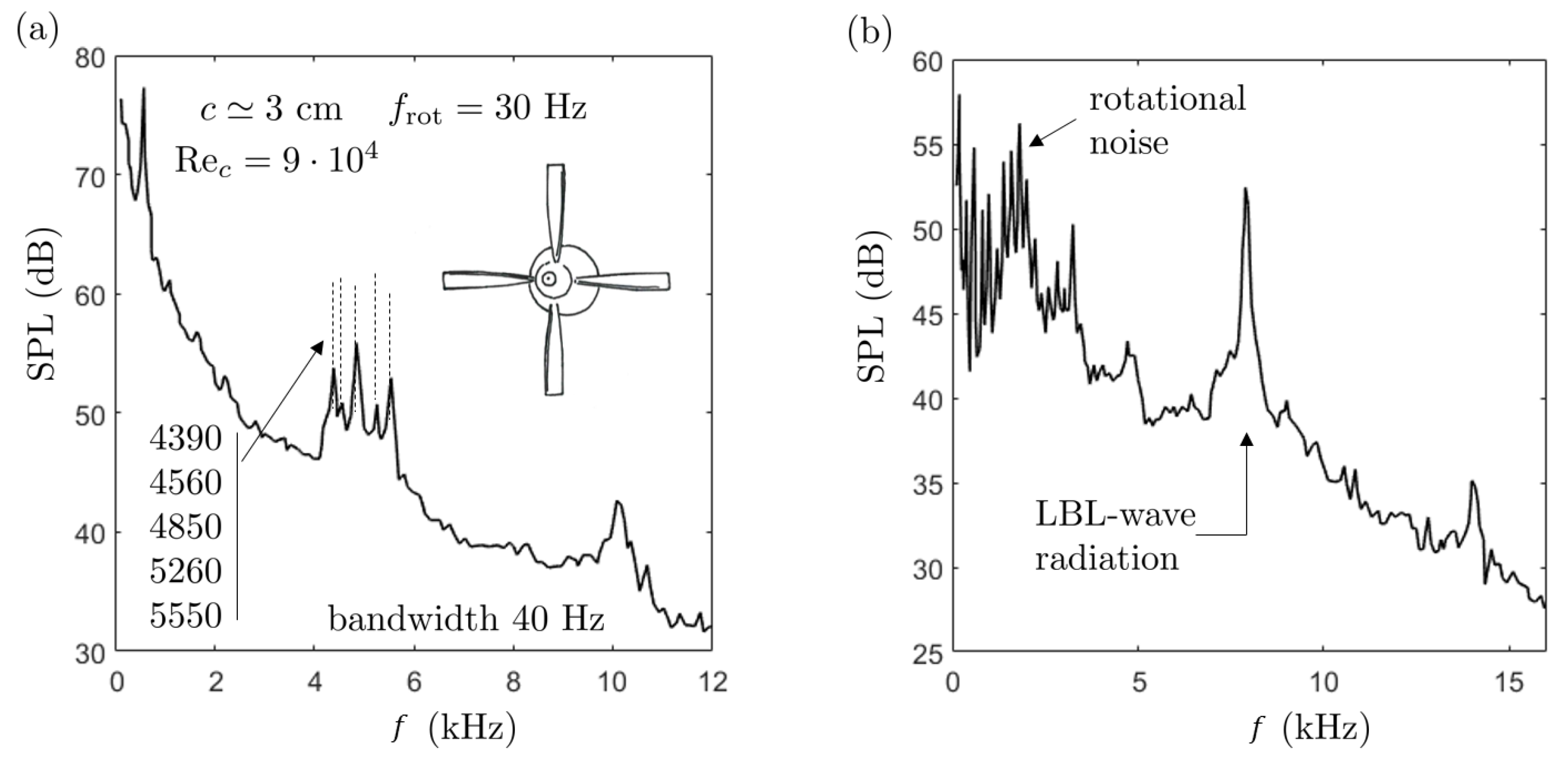
1], on the one hand, and of unpublished results for a small 9-bladed low-speed fan used for cooling electronic racks, on the other hand. Grosche and Stiewitt’s investigation refers to a four-bladed model propeller with a conventional blade design. The blades have a quite large aspect ratio. They are shown with the sound spectrum measured for some intermediate loading conditions of the blades using a mirror microphone in Figure 21, reproduced from the reference. The microphone is in the rotation plane. The spectrum features a clear narrow-band hump with several superimposed tones centered around 5 kHz as well as a harmonic hump around 10 kHz. This behavior is very similar to the signature of both aerofoils investigated in the present work for some speeds. However, the rotating motion causes an additional modulation of the actually emitted frequencies, which must be taken into account.
Longhouse [1] observed LBL-wave radiation in the experimental study of a low-speed four-bladed fan. Tests were performed with tripping to force transition to turbulence in the boundary layers on all blades, except for a small portion of span near the tip of a single blade. This ensured a laminar regime on this portion and highlighted the nearly-tonal signature. The quality of the flow was also checked visually with an acenaphthene mixture. A typical sound spectrum at reduced speed is shown in Figure 21b. It exhibits a single peak frequency but up to three frequencies are reported by Longhouse at higher speeds. The microphone is on axis in this case so that no rotation-induced modulation occurs, as emphasized below. Longhouse’s interpretation is compatible with the assumption of a feedback according to Equation (3) except that the term 1 / 2 is not considered. At the price of some adjustment it led to the orders n = 12, 13, and 14 for the measured tones. The fact that higher orders n only can be identified is confirmed by matching theoretical lines in Figure 6. Now in both aforementioned references there is no proof that the multiple tones are produced simultaneously. If they are, there is no clue of an underlying modulation mechanism other than the effect of rotation.
The aforementioned modulation effect can be assessed in both experiments. To this end, expressions for the Fourier transform of the far-field acoustic pressure for a rotating blade segment as provided in many handbooks, for instance [49], are reliable. If a compact blade segment of mean radius R 0 and coherent emission at the angular frequency ω 0 are assumed, this transform reads
p ( x , ω ) = i k F 0 e i k R 4 π R n = ( i ) n e i n ϕ J n ( k R 0 sin θ )
× cos γ cos θ n sin γ k R 0 δ ( ω [ ω 0 + n Ω ] ) ,
k = ω / c 0 being the acoustic wavenumber at angular frequency ω = 2 π f , Ω the rotational speed, γ the stagger angle of the blades as defined with respect to the rotational plane, F 0 the dipole source strength, and R the distance. The dipole character is strictly valid only at low frequencies but it is retained for simplicity in the present estimates. For an observer in the rotation plane, at 90 from the propeller axis as in Grosche and Stiewitt’s experiment the expression reduces to
p ( x , ω ) = i F 0 e i k R sin γ 4 π R R 0 n = ( i ) n e i n ϕ n J n ( k R 0 ) δ ( ω [ ω 0 + n Ω ] ) ,
which corresponds to the maximum amount of modulation, whereas for an on-axis observer, thus θ = 0 as in Longhouse’s experiment it reduces to
p ( x , ω ) = i k F 0 e i k R 4 π R cos γ δ ( ω ω 0 )
because only the term n = 0 contributes. No modulation occurs in this case. Therefore, the discussion now focuses on Grosche and Stiewitt’s experiment.
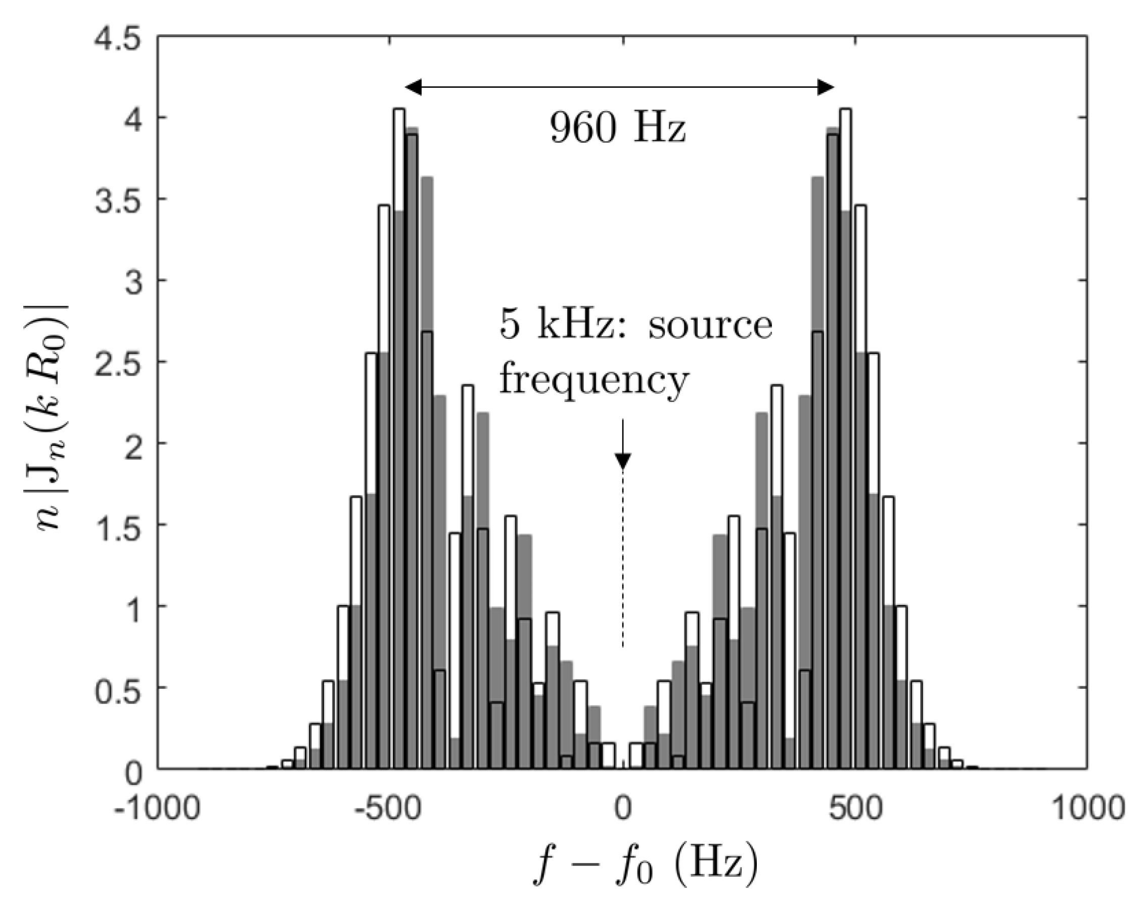
It can be guessed that the LBL waves are not blade-to-blade correlated, so that the main trends of the formula are not questioned if all blades are taken into account. The Dirac comb of angular frequencies ω 0 + n Ω is generated by the modulation but its envelope is determined by the function n J n ( k R 0 ) in Equation (11). This function is plotted in Figure 22 for values of R 0 of 88% and 92% of the tip radius in Grosche and Stiewitt’s experiment and the same parameters as in Figure 21a, in particular a source frequency f 0 = 5000 Hz. Arbitrarily selecting radii close to the blade-tip region is justified by the fact that the latter has low twist and is more likely to allow the onset of tonal noise. As a result that the frequency resolution of 40 Hz is higher than the modulating frequency of 30 Hz, it is expected to generate two peaks in the sound spectrum apart from the actually emitted frequency f 0 . The fact that the source frequency is not theoretically captured is because the term n = 0 is zero in the sum. Probably this is not so in the experiment because the mirror averages sounds emitted also at angles different from 90 ; in this case the more complete form of the expression, Equation (10) should be used. Yet, five tones are observed, the frequencies of which are indicated in Figure 21a. The theoretical peak-to-peak distance is around 960 Hz, which is smaller than the measured span of about 1160 Hz between the extreme tones in the figure. If only the first four or last four tones from the five are considered the value of 960 Hz is recovered. It is therefore concluded that more than just one tone is emitted by the blade segments responsible for the LBL-wave radiation. As a complement to the test illustrated in 
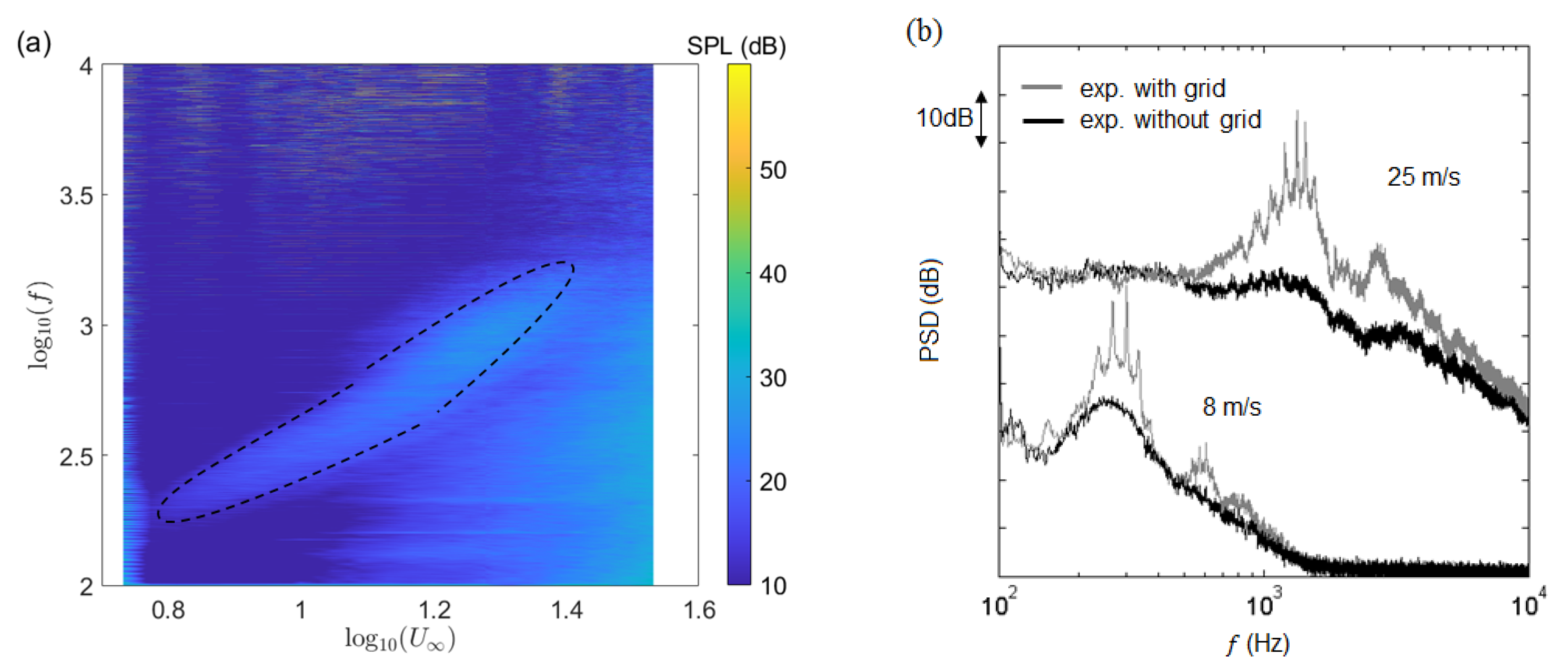
Figure 3, these results confirm that the present observations on isolated aerofoils are representative of true rotating-blade features and not deteriorated by installation effects. The similarity of the results is even surprising in view of the spanwise-variable conditions encountered on the propeller. The design of the blades makes their outer part nearly rectangular with no sweep and moderate twist [2]; therefore, only the tip region very likely experiences the favorable conditions for sustained LBL waves.
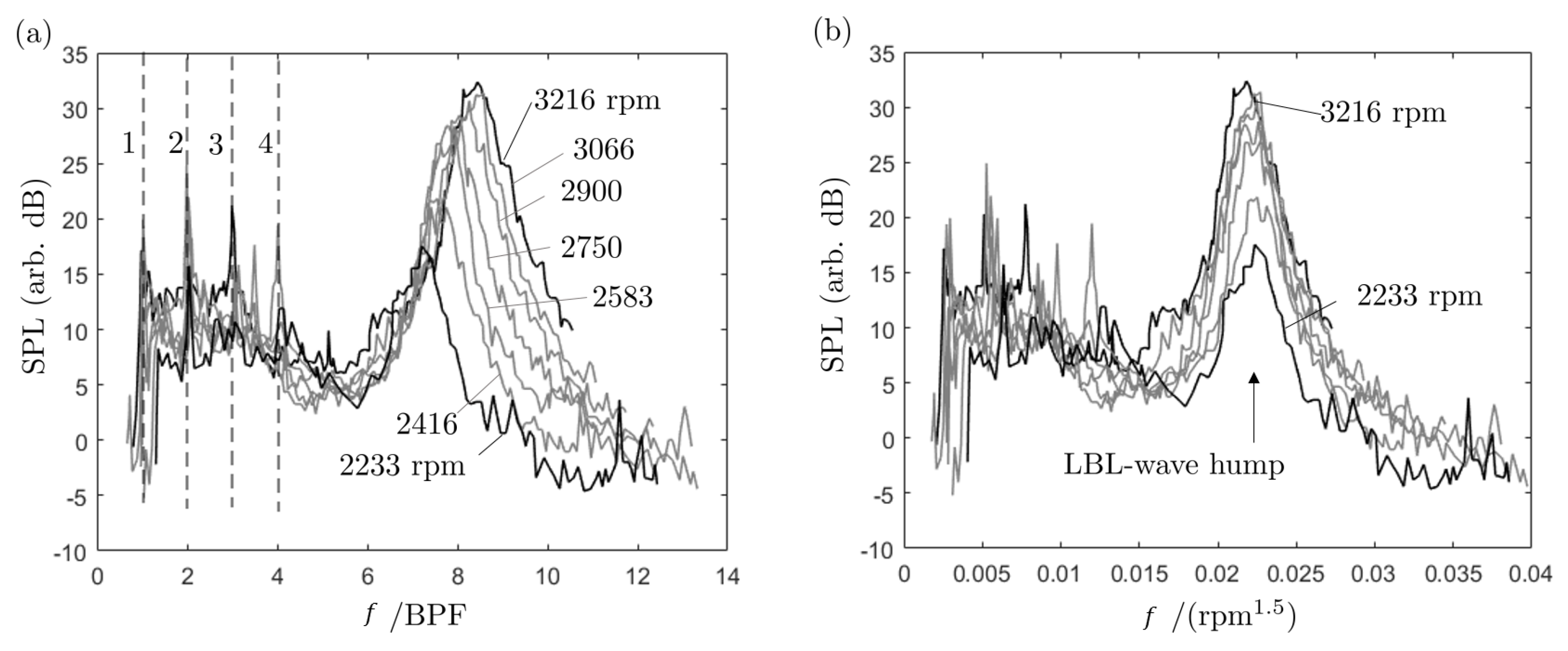
As a useful complement for the discussion, sound spectra of a small-size, axial-flow cooling fan for electronic equipments are reported in Figure 23, after the processing of additional data from Bridelance [50] by the authors. The measurements were made for a series of rotational speeds triggering nearly proportional relative speeds on the blades. The 9-bladed fan was mounted with an inlet bellmouth in a clean environment. It has a diameter of 145 mm and a hub-to-tip ratio of 0.6. In Figure 23a, the frequency is made dimensionless by the blade passing frequency (BPF), which leads to a clear identification of the first four BPF harmonics. The feature of interest is the higher-frequency hump, obviously of higher amplitude and shifted to higher frequencies as the rotational speed increases. If attributed to some von Kármán vortex shedding due to blade thickness at the trailing edge the hump would have a constant center frequency. Now scaling the frequency with the power 1.5 of the rotational speed leads to the plot in Figure 23b, where the hump is found at the same place for all speeds. Moreover, putting small tripping strips close to the suction-side leading edges of the blades has been found to suppress the spectral hump. This suggests that the hump is again produced by LBL-wave radiation. Yet, no tonal noise is observed. Reasons for that could be the non-homogeneous conditions along the quite short span of the blades, on the one hand, and sound scattering by the shroud of the fan and blade-to-blade proximity effects, on the other hand. The very small size of the blades might also be insufficient. The hump can be considered as the primary radiation of the instability waves, free of acoustic feedback, similar to the oblique trace in Figure 16.

5. Analytical Prediction of the Tonal Noise Emission

A two-dimensional analytical model of the trailing-edge scattering with acoustic feedback is justified by the inspection of signals delivered by the RMPs of the spanwise array discussed in Section 3.6.2. In this section, compressible Amiet’s theory is selected for its ability to provide two key results, namely an explicit expression for the acoustic wall-pressure generated by the scattering and another expression for the three-dimensional far-field sound in the mid-span plane. This allows estimating the acoustic forcing of the boundary layers from microphone measurements. Only some outcomes of the theory are presented here and details can be found in [38,48,51].
The accepted interpretation of the aerofoil tonal noise mechanism is that instability waves developing as an incompressible motion are driven by the acoustic waves they generate when interacting with the trailing edge. Now both the incompressible (hydrodynamic) and compressible (acoustic) motions have very different characteristic scales at the present low Mach numbers, typically below 0.12. The acoustic-to-hydrodynamic wavelength ratio is inversely proportional to the Mach number. As a result, the acoustic motion is nearly in phase over quite large portions of the aerofoil chord. Intuitively this is compatible with a feedback between some starting point A and the trailing edge only if the instabilities are receptive to acoustic forcing in the vicinity of A and not elsewhere. This condition is fulfilled as long as the instabilities grow exponentially to reach high amplitudes away from the point A and as the acoustic motion is at a somewhat intermediate level. In order to confirm the scenario, estimates of the orders of magnitude of the various involved motions are needed, resorting to relevant models and/or measured quantities. The instability growth and overall level can be inferred from wall-pressure measurements performed at various chordwise locations but such measurements are also including acoustic pressure. It can also be investigated from numerical simulations. The other measured quantity is the far-field sound at 90 from the streamwise direction in the mid-span plane. LBL-wave radiation is just a declination of trailing-edge noise, therefore any validated model of that noise can be used to quantify the source-to-sound relationship and therefore help to interpret various measurements [48].
Amiet’s solution is in two steps. The first step provides an expression for the unsteady pressure distribution induced along the aerofoil surface by the scattering of a hydrodynamic pressure gust into sound at the trailing edge. This distribution is the trace of the acoustic motion at the wall that is actually forcing the developing hydrodynamic instability waves. In the second step, the far-field pressure is calculated from this wall-pressure distribution by a radiation integral.
The present use of Amiet’s model is to confirm the nature of the measured wall-pressure close to the trailing edge and its cause-to-effect relationship with the far-field sound by calculating the former from the latter. This is attempted only for the tones, the two-dimensionality of the instabilities being a crucial point. Now Amiet’s model is usually used to predict broadband trailing-edge noise within the scope of a statistical analysis in which the spanwise correlation length is smaller than the wetted span, leading to a closed-form expression of the far-field pressure PSD [38]. In the present case of assumed perfect correlation a deterministic formulation is required, associating a single LBL wave at a given frequency to an isolated gust. If the back-scattering by the leading edge is ignored for simplicity, which is justified at high frequencies [38,48], the amplitude of the near-field wall pressure induced on the aft part of the aerofoil by trailing-edge scattering at the angular frequency ω simply reads
| p N F | = P 0 1 ( 1 i ) E B X
for some amplitude P 0 of the incident (hydrodynamic) pressure gust. In this expression B = a K ¯ + ( 1 M ) μ , K ¯ = ω c / ( 2 U ) , M = U / c 0 , μ = K ¯ M / β 2 , β = 1 M 2 , X = x / c being the negative coordinate with origin at the trailing-edge made dimensionless by the half chord and a = U / U c being the ratio of the external flow speed to the convection speed of the hydrodynamic disturbances. E is the Fresnel integral defined as
E ( ξ ) = 0 e i t 2 π t d t .
This first step defines the trace of a cylindrical wave at the wall acting as a forcing term for the developing instability. No transient is considered so that it is assumed that the instability has reached its saturation level.
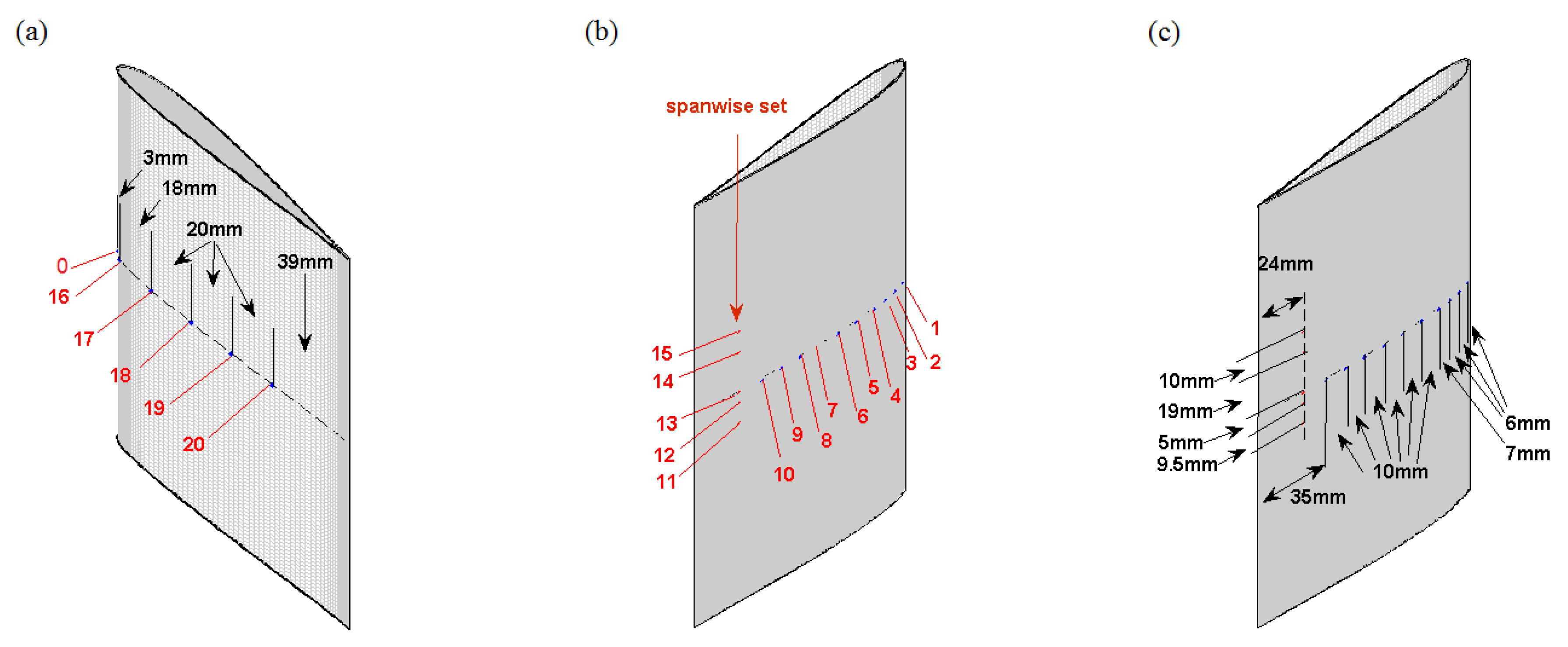
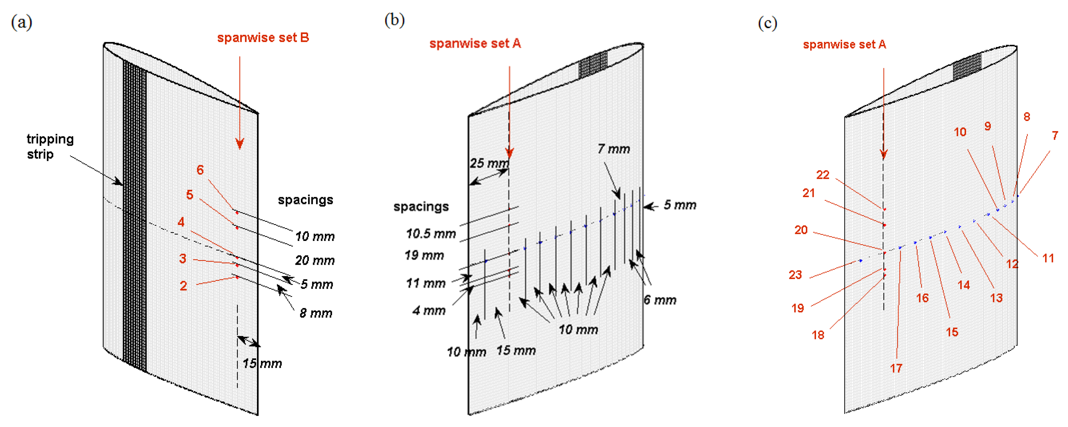
The main concern with the practical application of Equation (13) is that the amplitude P 0 
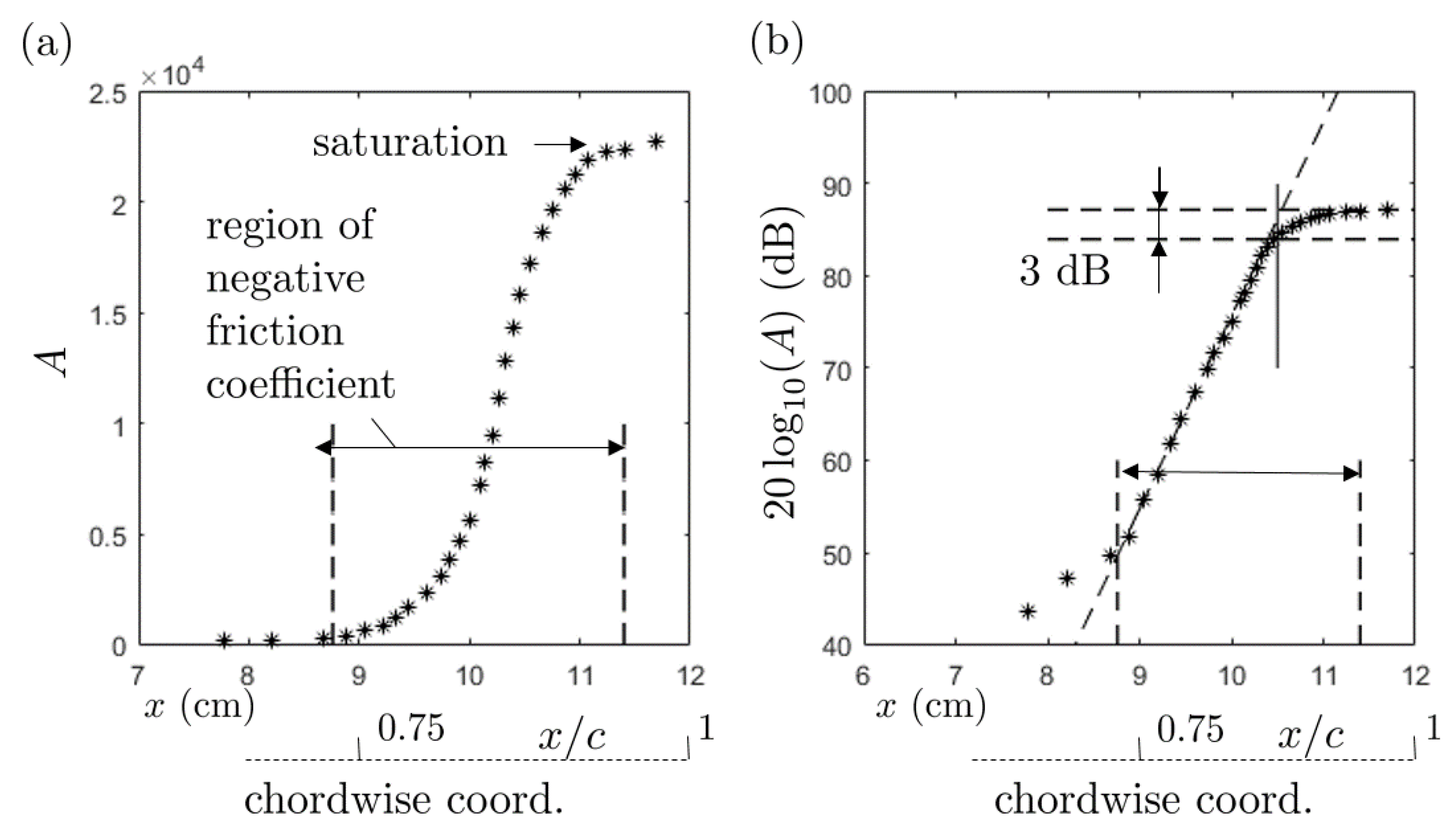
of the pressure gust that acts as an input should be taken just before the trailing edge whereas it is only measured 15 mm away from the trailing edge for the set B on the NACA-0012 aerofoil, thus at 87.5% of chord. The convection speed is also needed; it could be deduced with some approximation from the cross-spectrum phase calculated for the last chordwise RMP pair. Numerical simulations and computations based on the linear stability theory performed at 25 m/s by Nguyen et al. [27] are used in the present work to assess the relevance of the analytical modeling. Key results are reproduced in Figure 24 for the frequency of 1550 Hz corresponding to one of the emitted tones. The amplification of the oscillations as predicted with the linear stability theory is plotted in linear scale in Figure 24a and in logarithmic scale in Figure 24b. The amplitude unit is arbitrary because only relative variations are considered. The rapid growth takes place in the range of negative predicted friction coefficient thus in the separation area and leads to a saturation when approaching the trailing edge. Expressed in equivalent decibels the growth is approximately 21 dB per cm. The location of the last RMP is pointed out by the vertical line at x = 10.5 cm where the saturation starts. The plot indicates that the amplitude measured by the RMP must be increased by 3 dB to get a correct estimate of the gust at the trailing edge where the scattering as sound occurs. This makes sense only if the measurement is of purely hydrodynamic nature so that it can be considered as the relevant input in the analytical model. It is therefore essential to state about the relative levels of the developing instability and of the upstream-propagating sound wave for a clear assessment of the feedback. Furthermore, the same computations lead to convection speeds of about 40% of the external flow speed U to be used in the analytical solution.
The second step of the model leads to an approximation of the far-field pressure amplitude in the mid-span plane as [38]
| p F F | P 0 k H c 4 π C R 1 ( 1 i ) E 2 B + ( 1 i ) B μ e 2 i C E 2 μ
where C = a K ¯ + M 0 μ , H is the span length, R the microphone distance, and k the acoustic wavenumber. Forming the ratio | p N F | / | p F F | and multiplying by the amplitude of the measured far-field sound restores the needed acoustic trace on the wall as a function of the distance to the trailing edge (see 
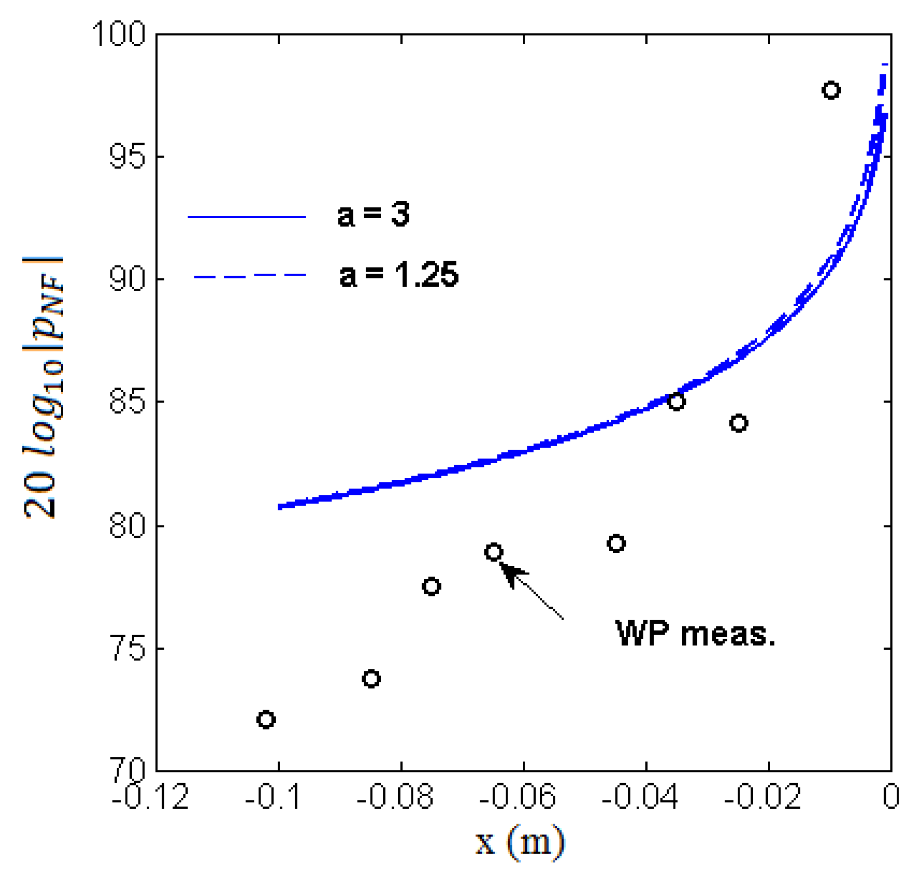
Figure 25). The parameter a strongly determines the amplitude of trailing-edge noise generation but it has a negligible effect on the aforementioned ratio. Indeed, it is given two values here, namely 3 and 1.25, without producing significant changes. The acoustic near-field is expected close to 100 dB directly upstream of the trailing edge, corresponding to the dominant tone. The near-field acoustic pressure is expected slightly above 80 dB around the location of point A according to this prediction. Unexpectedly the measured peak level at the wall is well below this value except in the aft part of the aerofoil whereas the RMP presumably capture the total pressure field, combining acoustic and hydrodynamic pressures.
The estimate must be taken with care because of ignored effects that are expected to occur close to the wall. The mean-velocity gradient in the boundary layer is responsible for refraction of upstream-propagating sound waves away from the wall. This possibly explains the results of Figure 25. Another point is that as the trailing-edge scattered pressure combines with the incident pressure, the phase shift of π presented in Equation (3) tends to produce a cancelling of the total pressure. This could also explain the unexpected misfit. Anyway, in view of the results the growing instabilities are probably not receptive to acoustic forcing in the last 30% of chord. However, they could be forced farther upstream. This makes the hypothesis of a feedback loop physically acceptable.
When addressing quantitative sound predictions from a specified amplitude in the hydrodynamic field, the convection speed must be known with a reasonable accuracy. Facing the difficulty of determining it for tones by the usual examination of the phases of cross-spectra between chordwise distributed sensors, the aforementioned stability calculations performed at ERAU [27,
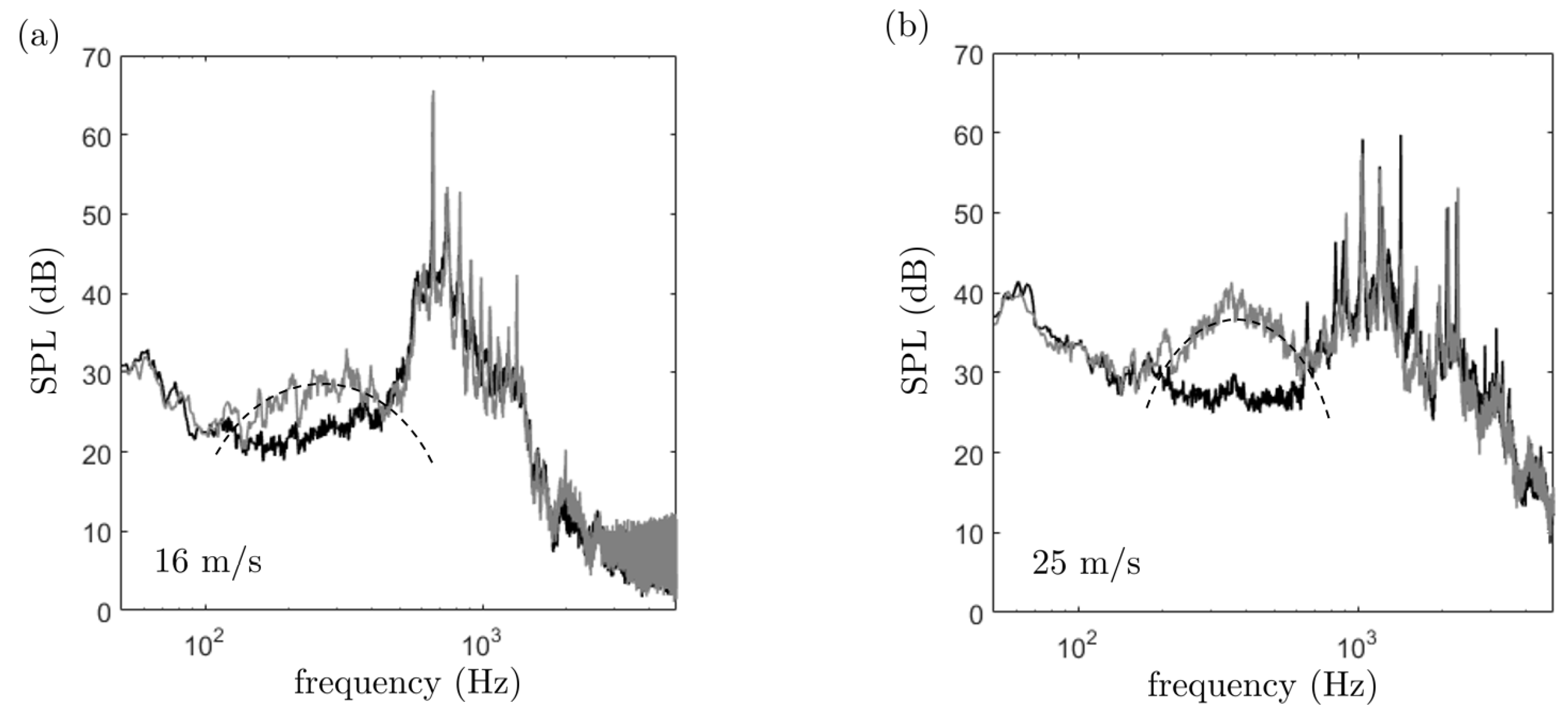
28] have been used instead. The theoretical convection speed is found below 30% of the external flow speed in the trailing-edge area. Higher convection speeds of 50% and 70% more representative of attached turbulent boundary layers have also been tested, leading to a range of values that can be interpreted as an uncertainty in the input data. Moreover, the analytical prediction from the measured wall spectra is made difficult for various reasons. Firstly, both sides of the aerofoil contribute, therefore calculations are to be performed for each; but the way the contributions interfere is not elucidated. Secondly, the wall pressure is measured only at some distance upstream of the trailing edge, whereas the instability waves are continuously amplified (or possibly damped) down to the trailing edge where they are scattered as sound. This makes some underestimate (or overestimate) expected. Finally, the reattachment of the separated layers in the very vicinity of the trailing edge presumably modifies the properties of the noise emission. Despite these questionable points, tone-level prediction have been attempted for the NACA-0012 aerofoil at the two flow speeds of 16 and 25 m/s taking the wall-pressure tone levels measured at RMP 4 (right-bank) and 23 (left-bank) as input data. This provides estimated values of the far-field sound that must be compared to the microphone measurements.
At 16 m/s the results are reported in Table 4. The tone at 556 Hz is only related to the right-bank side probe, as a result of the imbalance between both sides attributed to the installation. The dominant tone at 635 Hz is emitted from both sides with nearly equivalent source levels, though the overall wall-pressure level at probe 4 is lower than that at probe 23. This level difference is also possibly attributed to the larger distance of 15 mm (instead of 10 mm) to the edge at RMP location 4 (see Figure 4). The associated measured sound levels are 49 and 61.5 dB for the lower and the higher frequencies, respectively. Amiet’s model predicts sound levels ranging from 47.2 to 51 dB at 556 Hz for the extreme values of convection speeds 0.29 U and 0.7 U , higher convection speeds leading to higher sound predictions. At 635 Hz, the predictions range from 60.3 to 64 and from 62 to 66 dB depending on either the input data are considered at RMP 4 or RMP 23, respectively. In most cases, a slight over-prediction takes place. It is worth noting that both the developing boundary layers on the end plates and additional plate-aerofoil junction effects reduce the spanwise extent over which the laminar unstable regime takes place. Indeed the laminar instabilities are associated with the separation areas. This can be globally estimated from flow visualizations made with oil mixture as about 2.5 cm of attached flow at both junctions. The effective span length would be 25 cm instead of 30 cm according to this argument, which makes a sound-level reduction of about −16 dB expected. This makes the comparison quite satisfactory.
Surprisingly the same test repeated at 25 m/s (see Table 5) leads to larger overestimates. Indeed, for the frequencies 1200 Hz and 1333 Hz the measured tone levels are 50 and 55.6 dB whereas the predictions produced by both probe inputs range from 55 to 59 dB and from 62 to 69 dB, respectively. As can be seen at this flow velocity the over-prediction is systematic. It is not excluded (though not proved) that between the wall-pressure measurement point and the trailing edge, some reduction of the amplitude of the laminar boundary layer waves operates in this case.

6. Conclusions

The present study was aimed at getting a deeper understanding of the underlying physics of aerofoil tonal trailing-edge noise, as a basis for noise reduction or analytical prediction. A complete experimental database has been built for the NACA-0012 aerofoil and for the cambered SD7003 aerofoil. Though numerical predictions were also included in the collaborative research project, the present paper is mostly focused on the experimental and analytical results.
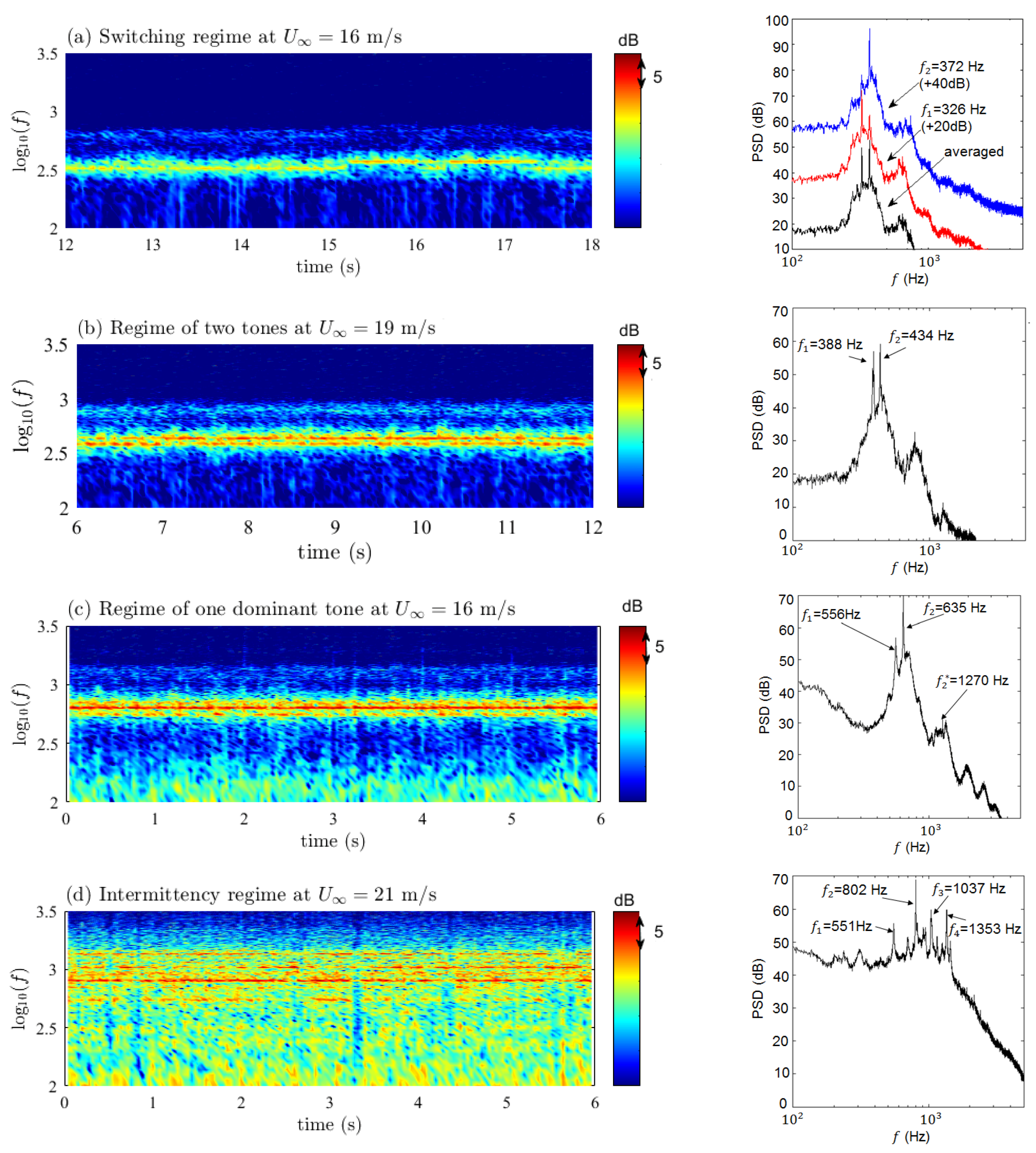
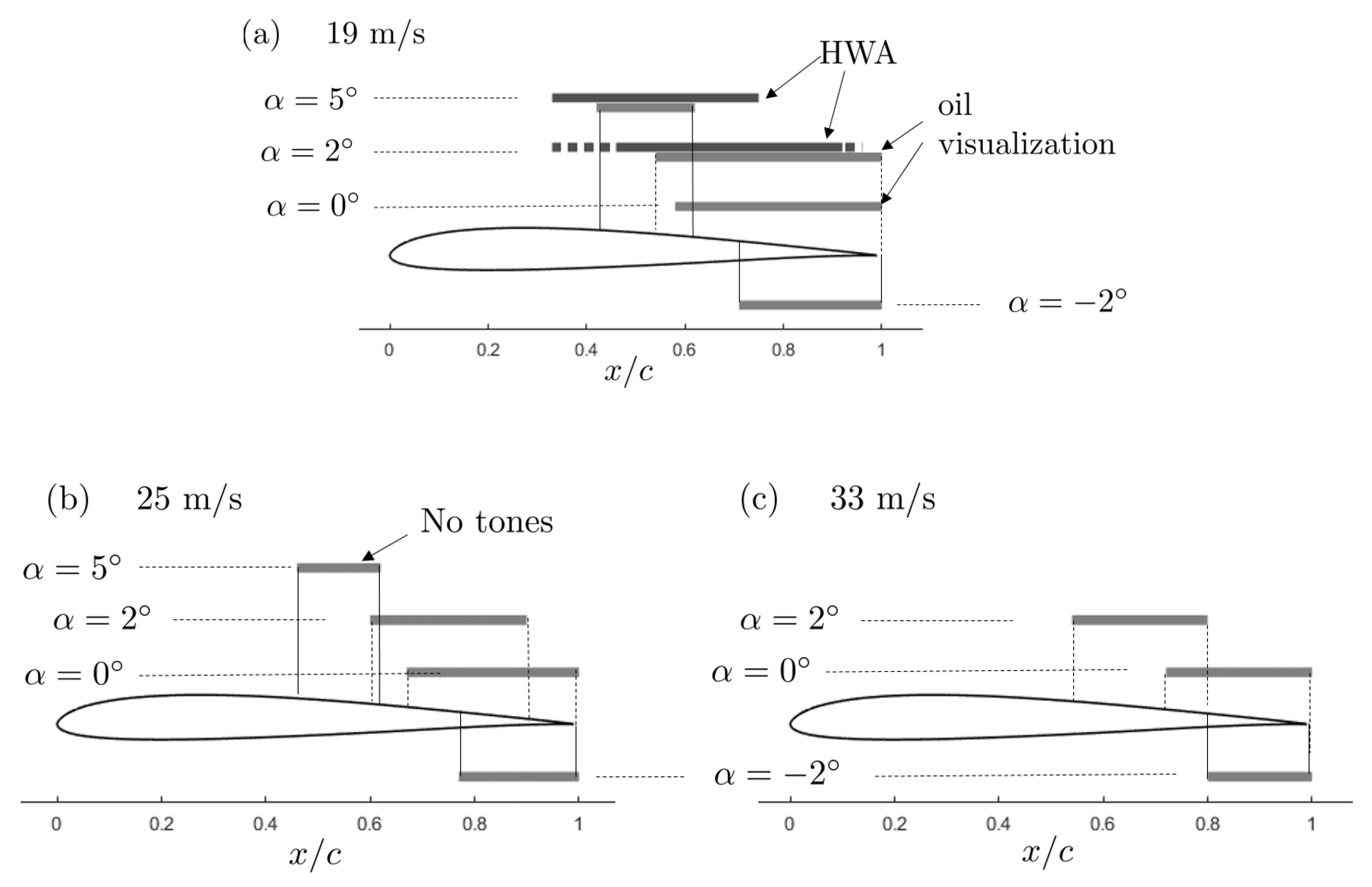
Far-field sound-pressure measurements performed at various flow speeds and geometrical angle of attack allowed pinpointing the limits of the tonal-noise emission area in the angle of attack and Reynolds number plane, showing both similarities and some differences with previously reported studies. This suggests the high sensitivity of the mechanism to experimental conditions. The SD7003 aerofoil is found to have a much narrower emission area than the NACA-0012. The measurements confirmed the “ladder-type” structure featured when plotting the variation of the dominant tone with increasing flow speed, for both aerofoils, explained by an acoustic feedback. Several regimes of tone emission were observed, namely a switching regime between two tones that are not observed simultaneously, a regime with a single tone or two simultaneous tones and a regime of intermittency with multiple unstable tones. Again, these regimes take place for both aerofoils depending on the flow parameters. This multiplicity could be more deeply addressed in the future as a possible explanation for the discrepancies sometimes found between numerical simulations and experiments. Keeping in mind that the former often run over very short times except in the recent LBM direct numerical simulations. Supplementary results obtained for the low-speed fans and propellers confirm that the laminar-boundary-layer instabilities can also be one of the noise sources in such rotating machines.
Special attention was paid to the role of each side of an aerofoil in the tonal noise generation, typically by resorting to one-side boundary-layer tripping. For the NACA-0012 aerofoil, the suction side boundary-layer has been found responsible for the tone generation only at low geometrical angles of attack and velocities, whereas for higher values of these parameters the sound can be attributed to the pressure-side boundary layer. In the case of the SD7003 aerofoil, only the suction-side boundary layer contributes, the pressure-side one remaining laminar and stable. This confirms that a single laminar and unstable boundary layer is sufficient for the onset of tonal noise. In addition, the combination of the unstable boundary-layer with a very thin separation bubble is essential to sustain high-amplitude tone emission. This was verified by both hot-wire anemometry scanning of the boundary-layer profiles and by oil flow visualization. The condition for efficient tonal noise generation is that the separation bubble extends down to the trailing edge or close to it. The separation bubble acts as an amplifier for the boundary layer instabilities. As shown by accompanying numerical simulations not detailed here, the receptivity point for the acoustic feedback is the attached-flow area where Tollmien–Schlichting waves develop just upstream of the separation point. The acoustic feedback and the tone emission have been simply suppressed and replaced by a hump-like primary narrow-band emission of much lower amplitude, by imposing upstream small-scale and small-amplitude turbulence in the incident flow, without changing the nature of the separation bubble. This proves that the separation bubble is a necessary but not sufficient condition for the mechanism. The acoustic feedback loop that amplifies the boundary layer instabilities at some frequencies is also required.
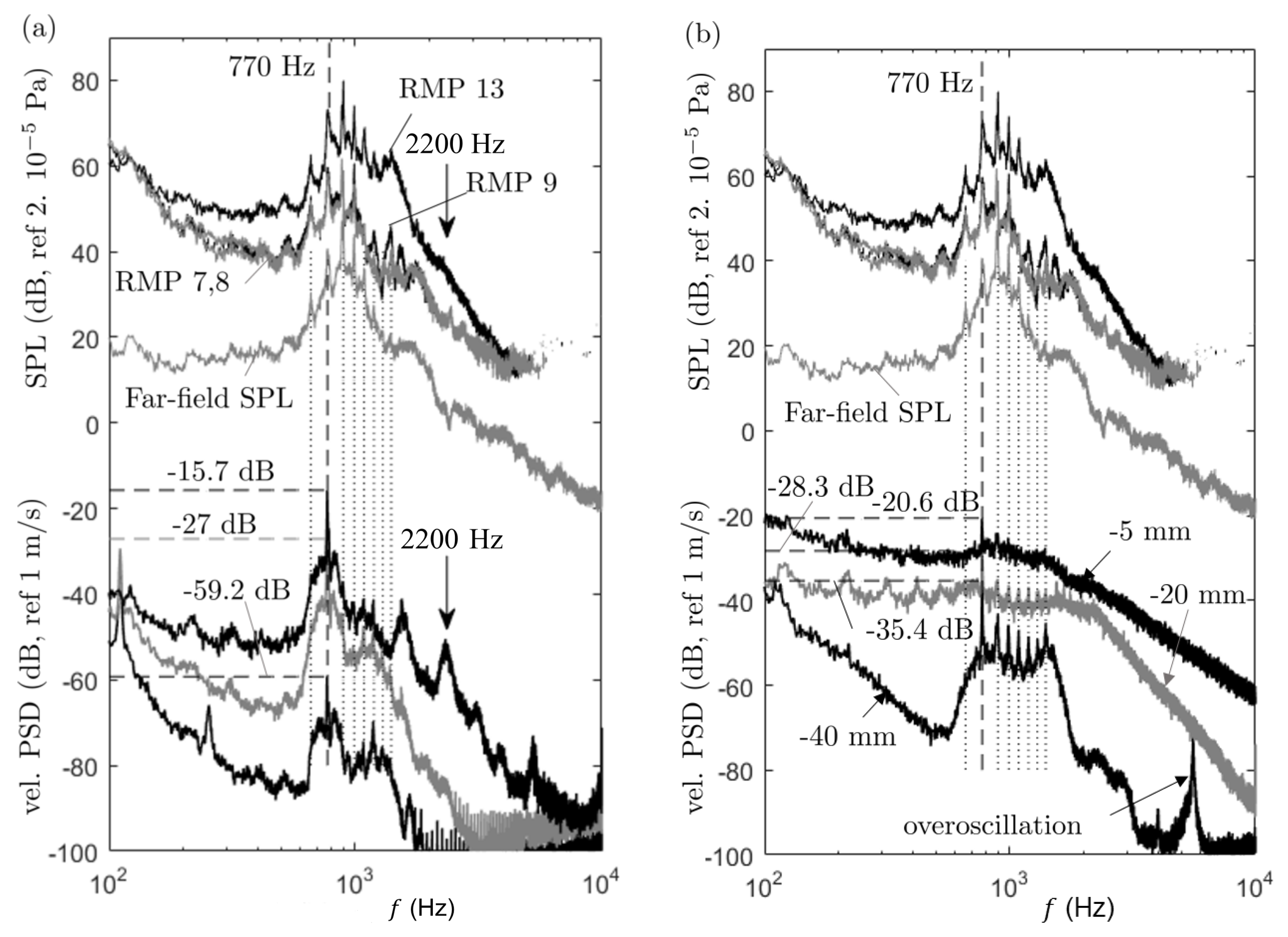
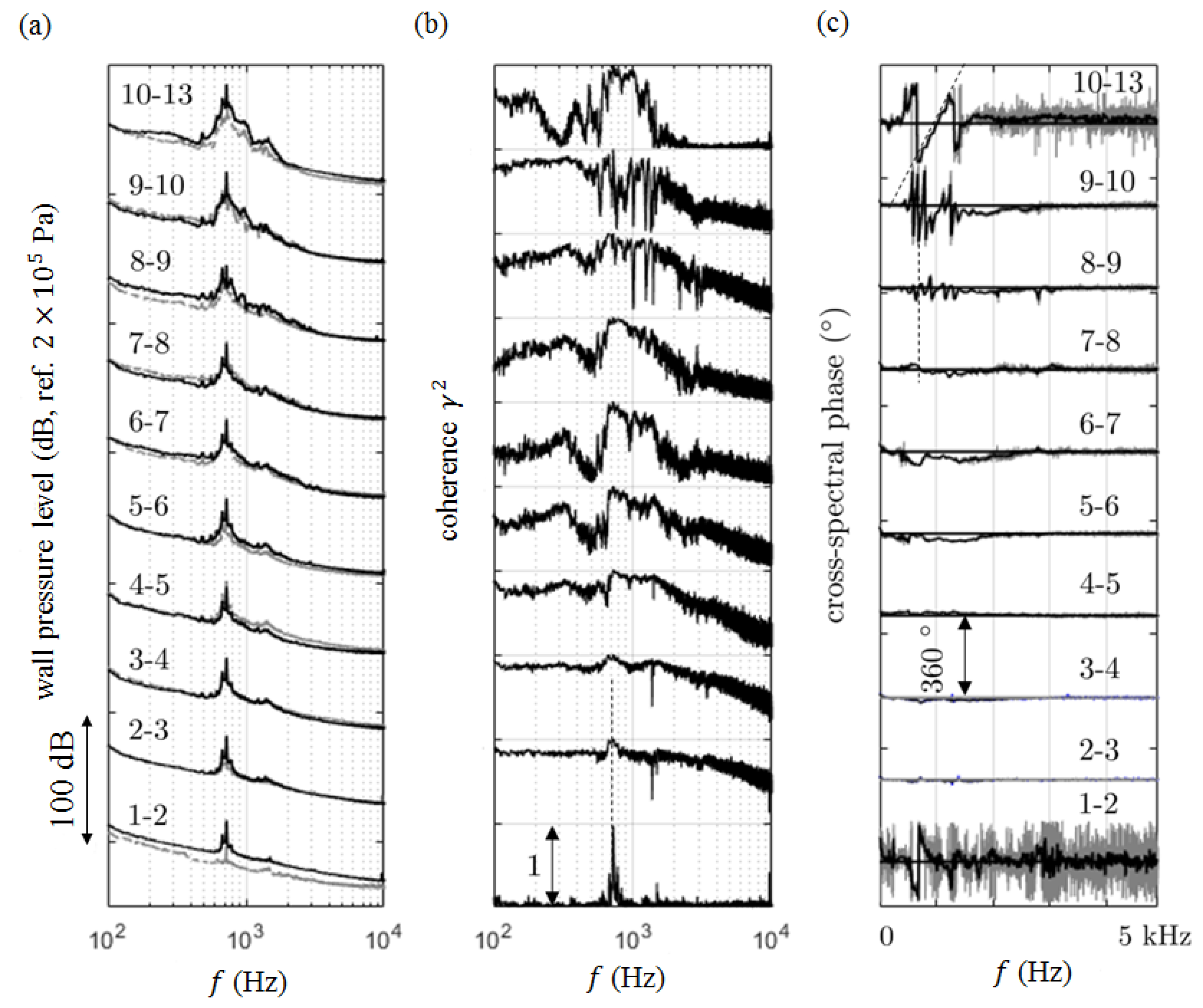
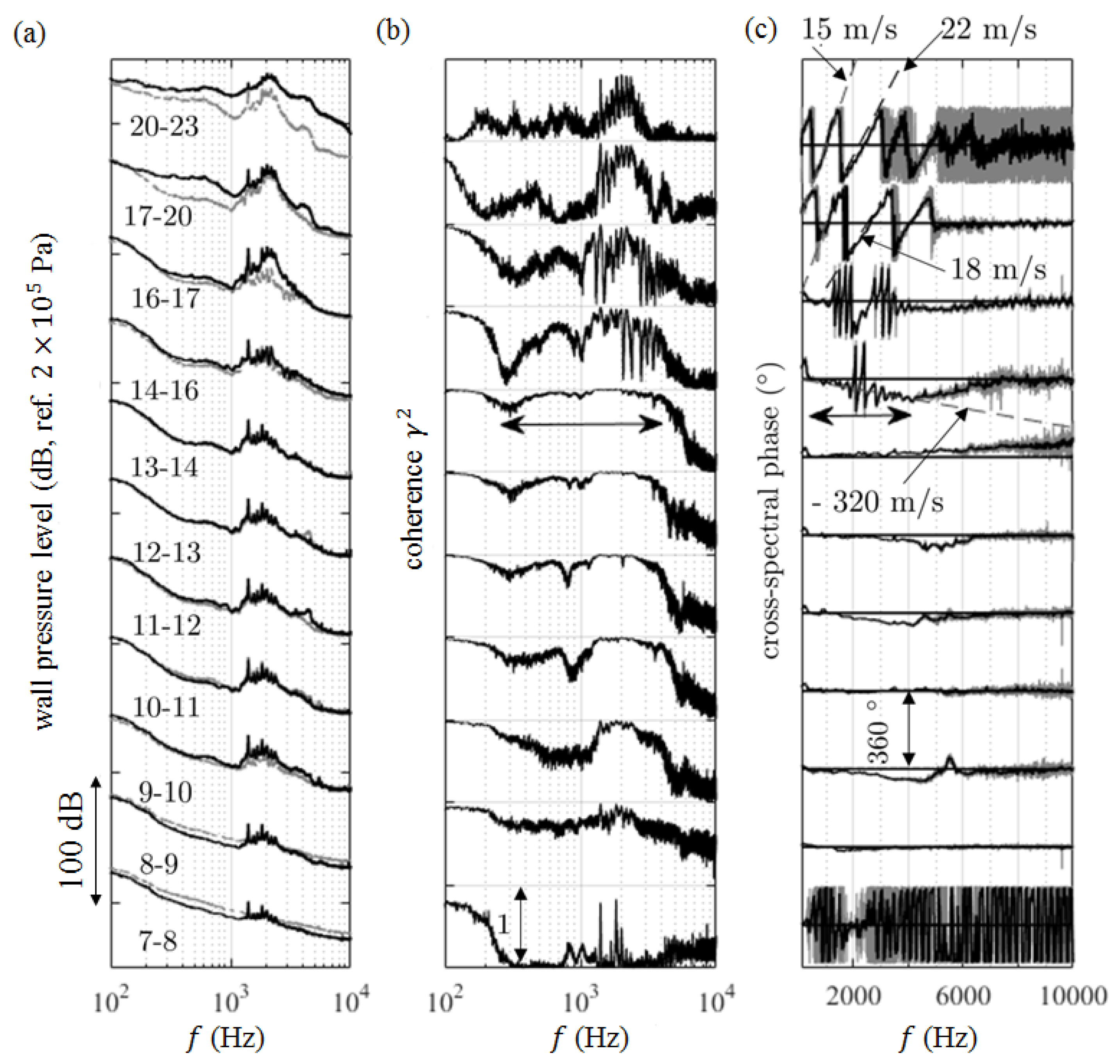
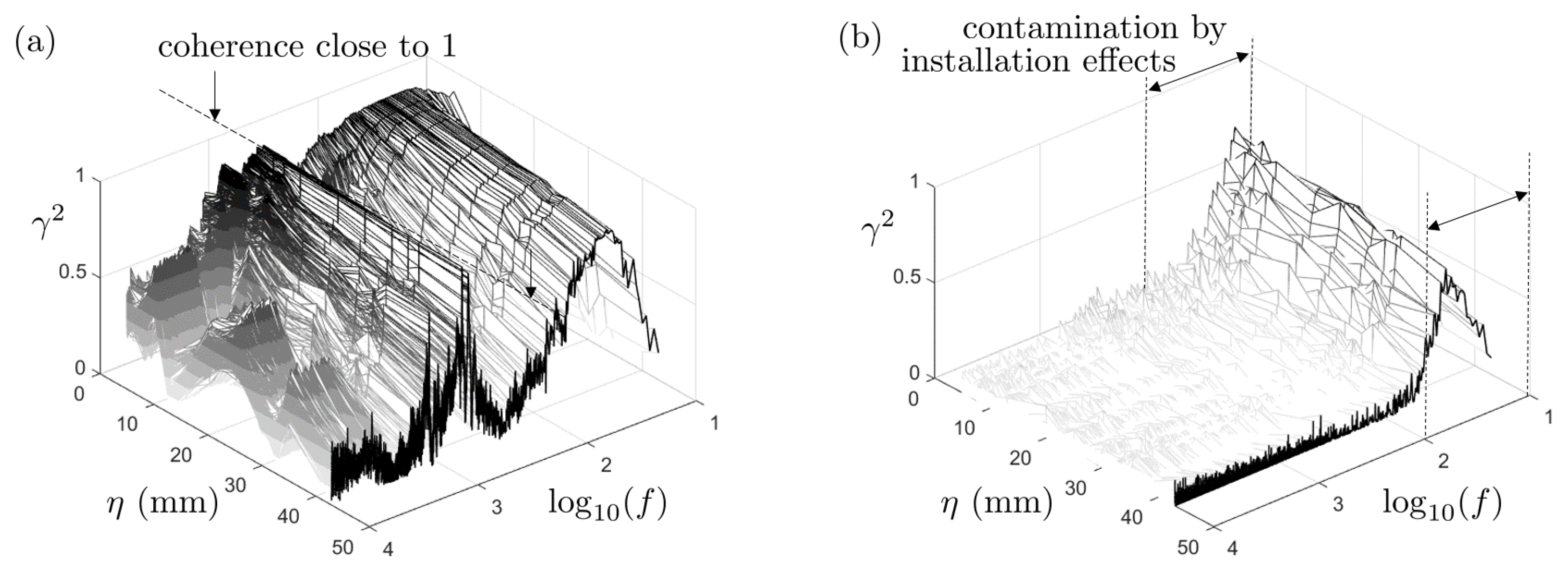
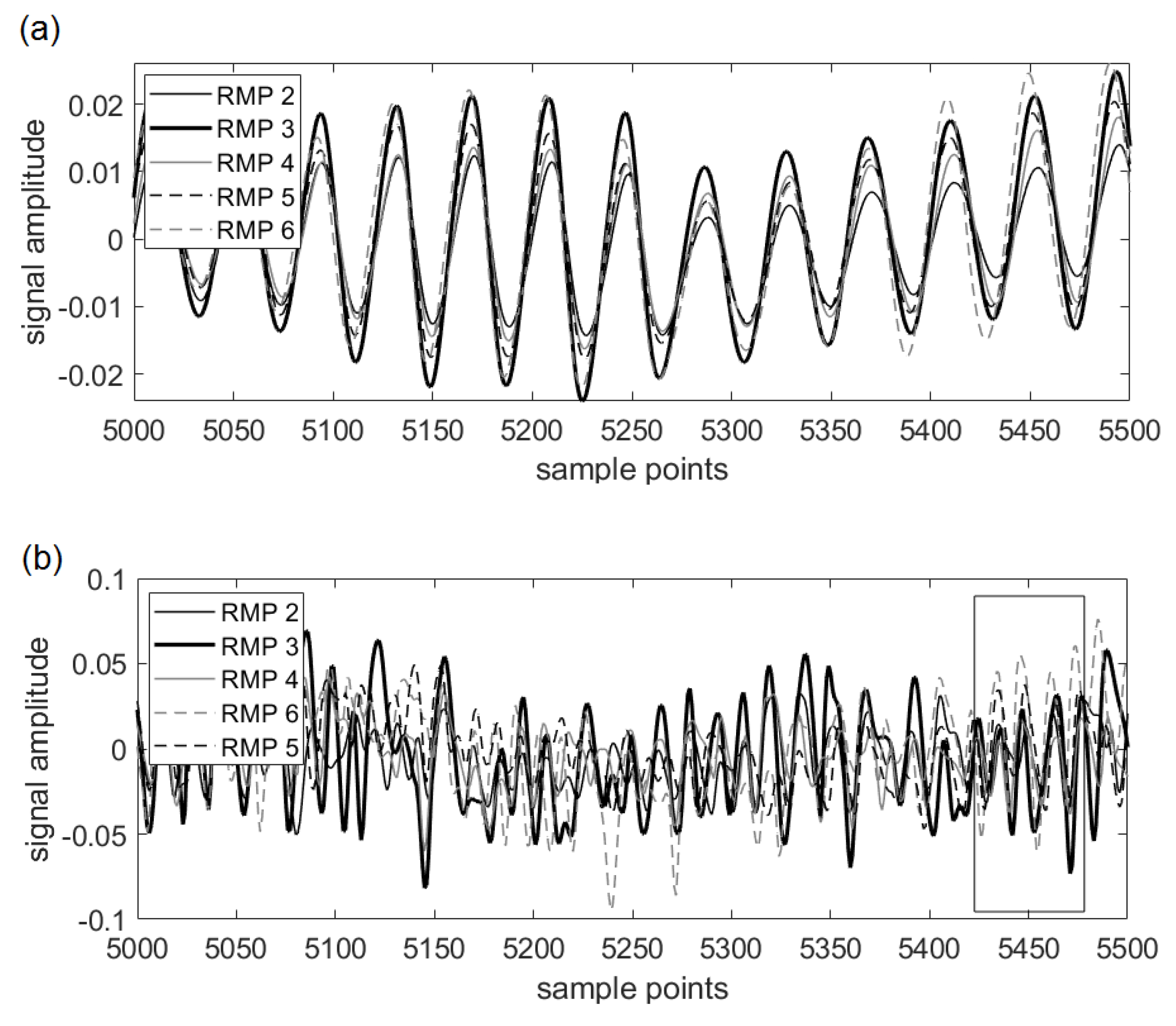
The cross-spectral analysis of chordwise located wall-pressure probes highlighted the highly coherent nature of the fluctuations at the frequencies of the tones. It also gave access to the convection speed of the instability waves used in analytical predictions. Furthermore, the analysis of the spanwise set of probes showed that the tones are associated with two-dimensional unstable motion. This is understood as a consequence of the acoustic feedback.
The analytical prediction of the tonal noise with an adapted Amiet’s model based on the measured surface pressure data acquired in the rear part of the aerofoil surface showed an overall satisfactory agreement with the measured tonal levels. It also confirms the cause-to-effect relationship between the wall pressure and the radiated sound. A possible cause of remaining discrepancies is the minimum distance of the last pressure probe to the trailing edge; indeed the instabilities can still evolve from that point to the trailing edge where they are scattered as sound.
Further analysis of the data base and/or additional investigations are needed to elucidate the physics underlying various emission regimes.

Author Contributions

Formal analysis, L.N.; Investigation, G.Y.; Supervision, M.R. and V.G.; Validation, L.N.; Writing—original draft, G.Y.; Writing—review and editing, M.R. and S.M. All authors have read and agree to the published version of the manuscript.

Funding

This research received no external funding.

Conflicts of Interest

The authors declare no conflict of interest.

References

  1. Longhouse, R.E. Vortex shedding noise of low tip speed, axial flow fans. J. Sound Vib. 1977, 53, 25–46. [Google Scholar] [CrossRef]
  2. Grosche, F.; Stiewitt, H. Investigation of Rotor Noise Source Mechanisms with Forward Speed Simulation. AIAA J. 1978, 16, 1255–1261. [Google Scholar] [CrossRef]
  3. Brooks, T.F.; Pope, D.S.; Marcolini, M.A. Airfoil Self-Noise and Prediction; Technical Report. 1989. Available online: https://ntrs.nasa.gov/archive/nasa/casi.ntrs.nasa.gov/19890016302.pdf (accessed on 20 March 2020).
  4. Fink, M.R. Prediction of airfoil tone frequencies. J. Aircr. 1975, 12, 118–120. [Google Scholar] [CrossRef]
  5. Paterson, R.W.; Vogt, P.G.; Fink, M.R.; Munch, C.L. Vortex noise of isolated airfoils. J. Aircr. 1973, 10, 296–302. [Google Scholar] [CrossRef]
  6. Tam, C.K. Discrete tones of isolated airfoils. J. Acoust. Soc. Am. 1974, 55, 1173–1177. [Google Scholar] [CrossRef]
  7. Arbey, H.; Bataille, J. Noise generated by airfoil profiles placed in a uniform laminar flow. J. Fluid Mech. 1983, 134, 33–47. [Google Scholar] [CrossRef] [Green Version]
  8. Desquesnes, G.; Terracol, M.; Sagaut, P. Numerical Investigation of the Tone Noise Mechanism over Laminar Airfoils. J. Fluid Mech. 2007, 591, 155–182. [Google Scholar] [CrossRef]
  9. Arcondoulis, E.; Doolan, C.J.; Zander, A.C.; Brooks, L.A.; Liu, Y. An investigation of airfoil dual acoustic feedback mechanisms at low-to-moderate Reynolds number. J. Sound Vib. 2019, 460, 114887. [Google Scholar] [CrossRef]
  10. Padois, T.; Laffay, P.; Idier, A.; Moreau, S. Tonal noise of a controlled-diffusion airfoil at low angle of attack and Reynolds number. J. Acoust. Soc. Am. 2016, 140, EL113–EL118. [Google Scholar] [CrossRef] [Green Version]
  11. Chong, T.; Joseph, P.; Kingan, M. An investigation of airfoil tonal noise at different Reynolds numbers and angles of attack. Appl. Acoust. 2013, 74, 38–48. [Google Scholar] [CrossRef]
  12. Nash, E.; Lowson, M.; McAlpine, A. Boundary-layer instability noise on aerofoils. J. Fluid Mech. 1999, 382, 27–61. [Google Scholar] [CrossRef]
  13. McAlpine, A.; Nash, E.; Lowson, M. On the generation of discrete frequency tones by the flow around an aerofoil. J. Sound Vib. 1999, 222, 753–779. [Google Scholar] [CrossRef] [Green Version]
  14. Golubev, V.; Nguyen, L.; Roger, M.; Visbal, M. On Interaction of Airfoil Leading and Trailing Edge Noise Sources in Turbulent Flow. In Proceedings of the 17th AIAA/CEAS Aeroacoustics Conference, Portland, OR, USA, 5–8 June 2011. [Google Scholar]
  15. Tam, C.K.; Ju, H. Aerofoil tones at moderate Reynolds number. J. Fluid Mech. 2012, 690, 536–570. [Google Scholar] [CrossRef]
  16. Lowson, M.; Fiddes, S.; Nash, E. Laminar Boundary Layer Aeroacoustic Instabilities. In Proceedings of the 32nd Aerospace Sciences Meeting and Exhibit, Reno, NV, USA, 10–13 January 1994. [Google Scholar]
  17. Inasawa, A.; Kamijo, T.; Asai, M. Generation mechanism of trailing-edge noise of airfoil at low Reynolds numbers. In Proceedings of the 13th Asian Congres of Fluid Mechanics, Dhaka, Bangladesh, 17–21 December 2010. [Google Scholar]
  18. Pröbsting, S.; Scarano, F.; Morris, S. Regimes of tonal noise on an airfoil at moderate Reynolds number. J. Fluid Mech. 2015, 780, 407–438. [Google Scholar] [CrossRef]
  19. Pröbsting, S.; Serpieri, J.; Scarano, F. Experimental investigation of aerofoil tonal noise generation. J. Fluid Mech. 2014, 747, 656–687. [Google Scholar] [CrossRef] [Green Version]
  20. Gerakopulos, R.; Yarusevych, S. Novel time-resolved pressure measurements on an airfoil at a low Reynolds number. AIAA J. 2012, 50, 1189–1200. [Google Scholar] [CrossRef]
  21. Padois, T.; Laffay, P.; Idier, A.; Moreau, S. Detailed Experimental Investigation of the Aeroacoustic Field around a Controlled-Diffusion Airfoil. In Proceedings of the 21st AIAA/CEAS Aeroacoustics Conference, Dallas, TX, USA, 22–26 June 2015. [Google Scholar]
  22. Sanjosé, M.; Jaiswal, P.; Arroyo, C.P.; Moreau, S.; Towne, A.; Lele, S.K.; Mann, A. Direct numerical simulation of laminar boundary layer instability noise. In Proceedings of the 23rd AIAA/CEAS Aeroacoustics Conference, Denver, CO, USA, 5–9 June 2017. [Google Scholar]
  23. Jaiswal, P.; Pasco, Y.; Moreau, S. Experimental investigation of airfoil tones on a CD airfoil. In Proceedings of the 27th CANCAM, Sherbrooke, QC, USA, 27–30 May 2019. [Google Scholar]
  24. Yakhina, G.; Roger, M.; Jondeau, E.; Golubev, V.; Nguyen, L. Parametric Investigations of Tonal Trailing-Edge Noise Generation by Moderate Reynolds Number Airfoils. Part I—Experimental Studies. In Proceedings of the 21st AIAA/CEAS Aeroacoustics Conference, Dallas, TX, USA, 22–26 June 2015. [Google Scholar]
  25. Yakhina, G.; Roger, M.; Kholodov, P.; Nguyen, L.; Golubev, V. An Integrated Study of Laminar Separation Bubble Effect on Tonal Noise Generation inTransitional Airfoils. In Proceedings of the 22nd AIAA/CEAS Aeroacoustics Conference, Lyon, France, 30 May–1 June 2016. [Google Scholar]
  26. Golubev, V.; Nguyen, L.; Hyner, W.; Sansone, M.; Salehian, S.; Mankbadi, R.; Yakhina, G.; Roger, M. Parametric Investigations of Tonal Trailing-Edge Noise Generation by Moderate Reynolds Number Airfoils. Part II—Numerical Studies. In Proceedings of the 21st AIAA/CEAS Aeroacoustics Conference, Dallas, TX, USA, 22–26 June 2015. [Google Scholar]
  27. Nguyen, L.; Golubev, V.; Mankbadi, R.; Yakhina, G.; Roger, M.; Visbal, R.M. A Summary of High-Fidelity Numerical Studies of Flow Acoustic Resonant Interaction in Transitional Airfoils. In Proceedings of the 22nd AIAA/CEAS Aeroacoustics Conference, Lyon, France, 30 May–1 June 2016. [Google Scholar]
  28. Nguyen, L.; Golubev, V.; Mankbadi, R.; Yakhina, G.; Roger, M.; Pasiliao, C.; Visbal, R.M. On Ladder-Type Structure of Acoustic Tones Radiated by Transition Airfoils. In Proceedings of the 23nd AIAA/CEAS Aeroacoustics Conference, Denver, CO, USA, 5–9 June 2017. [Google Scholar]
  29. Moreau, S.; Henner, M.; Iaccarino, G.; Wang, M.; Roger, M. Analysis of Flow Conditions in Freejet Experiments for Stuying Airfoil Self-Noise. AIAA J. 2003, 41, 1895–1905. [Google Scholar] [CrossRef]
  30. Moreau, S.; Roger, M. Effect of airfoil aerodynamic loading on trailing edge noise sources. AIAA J. 2005, 43, 41–52. [Google Scholar] [CrossRef] [Green Version]
  31. Roger, M.; Moreau, S. Broadband self noise from loaded fan blades. AIAA J. 2004, 42, 536–544. [Google Scholar] [CrossRef]
  32. Moreau, S.; Schram, C.; Roger, M. Diffraction Effects on the Trailing Edge Noise Meaasured in an Open-Jet Anechoic Wind Tunnel. In Proceedings of the 13th AIAA/CEAS Aeroacoustics Conference (28th AIAA Aeroacoustics Conference), Rome, Italy, 21–23 May 2007; p. 3706. [Google Scholar]
  33. Perennes, S.; Roger, M. Aerodynamic noise of a two-dimensional wing with high-lift devices. In Proceedings of the 4th AIAA/CEAS Aeroacoustics Conference, Toulouse, France, 2–4 June 1998; pp. 98–2338. [Google Scholar]
  34. Pérennès, S. Caractérisation des Sources de Bruit Aérodynamique à Basses Fréquences de Dispositifs Hypersustentateurs. Ph.D. Thesis, Ecole Centrale de Lyon, Écully, France, 1999. [Google Scholar]
  35. Salze, É.; Bailly, C.; Marsden, O.; Jondeau, E.; Juvé, D. An experimental characterization of wall pressure wavevector-frequency spectra in the presence of pressure gradients. In Proceedings of the 20th AIAA/CEAS Aeroacoustics Conference, Atlanta, GA, USA, 16–20 June 2014. [Google Scholar]
  36. Mueller, T.J. Aeroacoustic Measurements; Springer: New York, NY, USA, 2002. [Google Scholar]
  37. Brooks, T.F.; Hodgson, T.H. Trailing edge noise prediction from measured surface pressures. J. Sound Vib. 1981, 78, 69–117. [Google Scholar] [CrossRef]
  38. Roger, M.; Moreau, S. Back-scattering correction and further extensions of Amiet’s trailing-edge noise model. Part 1: Theory. J. Sound Vib. 2005, 286, 477–506. [Google Scholar] [CrossRef]
  39. Moreau, S.; Sanjosé, M.; Lyu, B.; Ayton, L.J. Analytical, numerical and experimental investigation of trailing-edge noise reduction on a Controlled Diffusion airfoil with serrations. In Proceedings of the 25th AIAA/CEAS Aeroacoustics Conference, Delft, The Netherlands, 20–23 May 2019; p. 2450. [Google Scholar]
  40. Sanjose, M.; Towne, A.; Jaiswal, P.; Moreau, S.; Lele, S.; Mann, A. Modal analysis of the laminar boundary layer instability and tonal noise of an airfoil at Reynolds number 150,000. Int. J. Aeroacoust. 2019, 18, 317–350. [Google Scholar] [CrossRef]
  41. Saric, W.S.; Reed, H.L.; White, E.B. Stability and transition of three-dimensional boundary layers. Annu. Rev. Fluid Mech. 2003, 35, 413–440. [Google Scholar] [CrossRef] [Green Version]
  42. Chong, T.; Joseph, P. Ladder Structure in Tonal Noise Generated Around an Airfoil. JASA 2012, 131, 1–7. [Google Scholar] [CrossRef] [PubMed] [Green Version]
  43. Nguyen, L. Tonal Noise Generation by Moderate Reynolds Number Airfoil. Ph.D. Thesis, Embry Riddle University, Daytona Beach, FL, USA, 2016. [Google Scholar]
  44. Kingan, M.J.; Pearse, J.R. Laminar boundary layer instability noise produced by an aerofoil. J. Sound Vib. 2009, 322, 808–828. [Google Scholar] [CrossRef]
  45. Arbey, H. L’étude des Mécanismes de L’émission Sonore de Profils Aérodynamiques Placés dans Des écoulements Sains ou Perturbés. Ph.D. Thesis, Université Claude Bernard, Lyon, France, 1981. [Google Scholar]
  46. Obremski, H.; Morkovin, M.V.; Landahl, M.; Wazzan, A.; Okamura, T. A Portfolio of Stability Characteristics of Incompressible Boundary Layers; Technical Report; Advisory Group for Aerospace Research and Development: Neuilly-Sur-Seine, France, 1969. [Google Scholar]
  47. Arcondoulis, E.; Doolan, C.; Zander, A. Airfoil noise measurements at various angles of attack and low Reynolds number. In Proceedings of the ACOUSTICS, Adelaide, Australia, 23–25 November 2009; pp. 23–25. [Google Scholar]
  48. Moreau, S.; Roger, M. Back-scattering correction and further extensions of Amiet’s trailing-edge noise model. Part II: Application. J. Sound Vib. 2009, 323, 397–425. [Google Scholar] [CrossRef]
  49. Goldstein, M.E. Aeroacoustics; Mc Graw-Hill: New York, NY, USA, 1976. [Google Scholar]
  50. Bridelance, J. Aeroacoustic Study of axial fans with small diameter: Analysis and suppression of instability noise. In Proceedings of the International Conference on Noise Control Engineering (InterNoise 86), Cambridge, MA, USA, 21–23 July 1986; pp. 141–146. [Google Scholar]
  51. Amiet, R.K. Noise due to Turbulent Flow Past a Trailing-Edge. J. Sound Vib. 1976, 43, 387–393. [Google Scholar] [CrossRef]
Figure 1. Tested aerofoil shapes in chordwise and normal coordinates ( x , y ) . Common chord length c = 12 cm.
Acoustics 02 00018 g001
Figure 2. Sketch of the experimental setup. View from right-bank side.
Acoustics 02 00018 g002
Figure 3. Far-field sound spectra measured normal to the flow direction in the mid-span plane with aerofoil alone (black) and with aerofoil and splitter-plate (grey). NACA-0012 aerofoil at zero angle of attack. (a) 16 m/s, (b) 25 m/s. Jet-splitter noise marked with the dashed arcs.
Acoustics 02 00018 g003
Figure 4. Pin-hole locations and probe labels of the wall-pressure Remote Microphone Probes (RMP) on the NACA-0012 mock-up. (a) Right-bank side; (b,c) left-bank side. Relative position of the tripping device on the right-bank side indicated as the black strip in subplot (a). Numbers of probes in red, spacing between probes in black.
Acoustics 02 00018 g004
Figure 5. Pin-hole locations and probe labels of the wall-pressure RMP on the SD7003 mock-up. (a) Pressure side; (b,c) suction side. Numbers of probes in red, spacing between probes in black.
Acoustics 02 00018 g005
Figure 6. Frequency-flow speed maps of Laminar-Boundary-Layer (LBL)-wave radiation for the NACA-0012 aerofoil at zero angle of attack (a) and for the SD7003 aerofoil at 2 geometrical angle of attack (b). Clean aerofoils. Dominant tone frequencies marked by red circles. 8 values of the flow speed in Table 1 featured by vertical segments. White-dotted lines generated by Equation (3).
Acoustics 02 00018 g006
Figure 7. Sound-pressure spectra extracted from the map in Figure 6b showing multiple tones for the SD7003 aerofoil. Values of the averaged frequency jumps for series of tones indicated on the plots (dashed vertical segments).
Acoustics 02 00018 g007
Figure 8. Time-frequency analysis, (left) spectrograms, (right) averaged far-field spectra; (a,b) for the SD7003 aerofoil and (c,d) for the NACA-0012 aerofoil at α = 0 . Note that for case (a), two averaged spectra are shown for the two states of the switching regime.
Acoustics 02 00018 g008
Figure 9. Frequency-versus-flow speed maps of LBL-wave radiation for the NACA-0012 aerofoil at α = 5 . (a) Tripping on the pressure side; (b) tripping on the suction side; (c) clean configuration. Dominant tone frequencies marked by red circles. Black and white arrows and segments pointing to the steps of the ladder-type structures in subplots (a,b) reproduced for comparison in (c).
Acoustics 02 00018 g009
Figure 10. Flow visualization (a) LE—leading edge, TE—trailing edge. Velocity profiles produced by the HWA (b) for the suction side of the SD7003 aerofoil at α = 2 and 19 m/s for which tonal noise is observed. Upper plots: mean velocity. Lower plots: rms velocity.
Acoustics 02 00018 g010
Figure 11. Separated-flow areas on the NACA-0012 aerofoil at geometrical angles of attack α = 0 (a), α = 5 ( α * = 1.75 ) (b), and α = 10 (c) for various flow speeds. Upper and lower sides as suction and pressure sides in subplots (b) and (c), respectively. HWA (dark bars) and oil-visualization (grey bars) results. Indicative simulation results at α * = 2 as black dotted lines [27].
Acoustics 02 00018 g011
Figure 12. Separated-flow areas on the suction side of the SD7003 aerofoil at geometrical angles of attack α = 2 , 0 , 2 , and 5 at 19 m/s (a), 25 m/s (b), and 33 m/s (c). HWA (dark bars) and oil-visualization (grey bars) results.
Acoustics 02 00018 g012
Figure 13. (a) Geometrical angle of attack versus Reynolds number for the NACA-0012 aerofoil and the SD7003 aerofoil. Filled circles show the limits of the tonal-noise regime; empty circles point to the onset of low-amplitude noise. Green area is the primary emission for the NACA-0012 aerofoil, red and orange areas are tonal noise generated by pressure or suction sides of the NACA-0012, respectively, grey area is tonal noise generated by suction side of the SD7003 aerofoil. (b) Effective angle of attack versus Reynolds number for the NACA-0012 aerofoil compared with previous investigations.
Acoustics 02 00018 g013
Figure 14. Compared velocity spectra from HWA (dB, ref.1 m/s), wall-pressure spectra from some RMPs and far-field acoustic spectrum (both dB, ref. 2 × 10 5 Pa) for the SD7003 aerofoil. Geometrical angle of attack 2 , U = 19 m/s. Pressure side (a) and suction side (b). Emphasis on the tone at 770 Hz.
Acoustics 02 00018 g014
Figure 15. Hot-wire velocity spectra (dB, ref.1 m/s) for the residual wind-tunnel turbulence and the grid-generated turbulence. Reference acoustic velocity levels indicated for sound pressure levels of 74 dB (0.1 Pa) and 94 dB (1 Pa). U = 25 m/s. Model von Kármán spectrum with parameters indicated on the plot.
Acoustics 02 00018 g015
Figure 16. (a) Frequency-flow speed chart for the NACA-0012 aerofoil at zero angle of attack with small-scale turbulence; (b) compared far-field sound spectra of the clean flow (grey) and with upstream turbulence (black). Flow speeds 8 m/s and 25 m/s. Both pairs of spectra are shifted by 20 dB from each other.
Acoustics 02 00018 g016
Figure 17. Signal processing for pairs of chordwise RMPs. (a) wall-pressure PSD in equivalent arbitrary decibels, first probe as grey dashed line, second one as black line. (b) Coherence plots shifted by 1 for clarity between adjacent pairs. (c) Phase of the cross-spectrum in linear frequency scale, with resolutions of 1 Hz (grey) and 8 Hz (black). Suction-side probes of the SD7003 aerofoil at α = 2 and U = 25 m/s.
Acoustics 02 00018 g017
Figure 18. Signal processing for pairs of chordwise RMPs. (a) Wall-pressure PSD in equivalent arbitrary decibels, first probe as grey dashed line, second one as black line. (b) Coherence plots shifted by 1 for clarity between adjacent pairs. (c) Phase of the cross-spectrum in linear frequency scale, with resolutions of 1 Hz (grey) and 8 Hz (black). NACA-0012 aerofoil at α = 0 and U = 30 m/s.
Acoustics 02 00018 g018
Figure 19. Spanwise-coherence surface for LBL-wave radiation with (a) and without (b) acoustic feedback (fine-grid turbulence). NACA-0012 aerofoil at U = 16 m/s and zero angle of attack. Right-bank side probes set B. Dashed line pointing to the dominant tone frequency. Frequency axis pointing from right to left for clarity.
Acoustics 02 00018 g019
Figure 20. Time signals from the spanwise set B of RMPs. NACA-0012 aerofoil at 16 m/s (a) and 30 m/s (b). Zero angle of attack.
Acoustics 02 00018 g020
Figure 21. Evidence of LBL-wave radiation from rotating blades. Grosche and Stiewitt’s [2] experiment (a) on a four-bladed model propeller at 1800 RPM and Longhouse’s [1] experiment (b) on a four-bladed low-speed fan at 4700 RPM.
Acoustics 02 00018 g021
Figure 22. Theoretical modulation spectra corresponding to Grosche and Stiewitt’s experiment [2]. Blade segments of radii 88% (grey bars) and 92% (empty bars) of the tip radius.
Acoustics 02 00018 g022
Figure 23. Evidence of non-tonal LBL-wave radiation from a small-scale low-speed fan at various rotational speeds. A-weighted sound levels. Scaling by the blade-passing frequency (a) and by the power 1.5 of the rotational speed (b).
Acoustics 02 00018 g023
Figure 24. Sample simulated growth of LBL instabilities on the NACA-0012 aerofoil with linear stability theory, from Nguyen et al. [27]. (a) Amplitude of oscillations in arbitrary units, as a function of the chordwise coordinate in the aft part of the aerofoil for 1550 Hz, showing saturation. Trailing edge at x = 12 cm. (b) Same data in logarithmic scale. Last RMP located at x = 10.5 cm (vertical segment). α = 0 , U = 25 m/s.
Acoustics 02 00018 g024
Figure 25. Estimation of the acoustic wall-pressure distribution from the far-field pressure, according to Amiet’s model (Equations (13) and (15)). Tone frequency of 800 Hz; flow velocity of 21 m/s; measured sound of 60 dB; distance of 1.5 m.
Acoustics 02 00018 g025
Table 1. Selected flow speeds and corresponding Reynolds numbers.
Nr.12345678
3 Speed U (m/s)811161921253033
Reynolds number R e ( × 10 5 ) 0.63 0.87 1.26 1.5 1.6 2 2.4 2.6
Table 2. Separation areas. Illustrative table for the NACA-0012 aerofoil. α geometrical angle of attack; U flow velocity; ss and ps suction and pressure sides, respectively; FV flow visualization; HWA hot-wire anemometry. The first value of the percentage points to the beginning of the separation area and the second one to the end.
U Side19 m/s25 m/s33 m/s
α FVHWAFVFV
0 54%, reversed42–92%54–85%57–80%
58–100%No tones
5 ss40–80%33–88%45–62%no measurement
33–79%
ps60–100%67–100%62%, reversedno measurement
10 ssno measurementno measurementno measurement10–17%
ps80%, reversed
Table 3. Separation areas. Illustrative table for the SD-7003 aerofoil. α geometrical angle of attack; U flow velocity; ss and ps suction and pressure sides, respectively; FV flow visualization; HWA hot-wire anemometry. The first value of the percentage points to the beginning of the separation area and the second one to the end.
U Side19 m/s25 m/s33 m/s
α FVHWAFVFV
0 ss58–100% 67–100%72–100%
psattached attachedattached
2 ss54–100%46–92%60–90%54–80%
psattached33–96%attachedattached
5 ,ss42–62%33–75%46–62%no measurement
No tonespsattached33–98%attachedno measurement
2 ss71%, reversedno measurement77%, reversed80%, reversed
psattachedno measurementattachedattached
Table 4. Tone levels as predicted with analytical modeling (AM) and measured in the far-field (FF). NACA-0012 aerofoil at 16 m/s and zero angle of attack. Probe numbers, related source levels (PSD) and convection speed are indicated.
Frequency 556 HzFrequency 635 Hz
PSD, dB U c / U AM, dBFF, dBPSD, dBAM, dBFF, dB
pr 494.40.2947.249107.260.361.5
0.549.662.7
0.75164.2
pr 23 0.29 109.262.3
0.564.7
0.766.2
Table 5. Tone levels as predicted with analytical modeling (AM) and measured in the far-field (FF). NACA-0012 aerofoil at 25 m/s and zero angle of attack. Probe numbers, related source levels (PSD), and convection speed are indicated.
Frequency 1200 HzFrequency 1333 Hz
PSD, dB U c / U AM, dBFF, dBPSD, dBAM, dBFF, dB
pr 499.60.2955.449.9109.565.156.7
0.557.867.5
0.759.369
pr 23 0.29 10762.6
0.565
0.766.5

