Time-Domain Output Data Identification Model for Pipeline Flaw Detection Using Blind Source Separation Technique Complexity Pursuit

Abstract

Vital defect information present in the magnetic field data of oil and gas pipelines can be perceived by developing such non-parametric algorithms that can extract modal features and performs structural assessment directly from the recorded signal data. This paper discusses such output-only modal identification method Complexity Pursuit (CP) based on blind signal separation. An application to the pipeline flaw detection is presented and it is shown that the complexity pursuit algorithm blindly estimates the modal parameters from the measured magnetic field signals. Numerical simulations for multi-degree of freedom systems show that the method can precisely identify the structural parameters. Experiments are performed first in a controlled laboratory environment secondly in real world, on pipeline magnetic field data, recorded using high precision magnetic field sensors. The measured structural responses are given as input to the blind source separation model where the complexity pursuit algorithm blindly extracted the least complex signals from the observed mixtures that were guaranteed to be source signals. The output power spectral densities calculated from the estimated modal responses exhibit rich physical interpretation of the pipeline structures.

1. Introduction

Pipelines are important channels of oil and gas transportation in many developing countries. They are made of ferromagnetic materials which are often vulnerable to corrosion and fatigue damages caused by surrounding environmental effects [1]. Early damage detection of buried steel pipelines is necessary to confirm safety and reliability during service conditions. To achieve such goals, the primary aim of this study is to develop a non-contact geomagnetic probe using basic principles of magnetic gradient tensor [2,3] to detect the geomagnetic field signals. Non-contact geomagnetic detection [4] is a new kind of non-destructive testing (NDT) technique that needs the Earth’s magnetic field as the stimulus source to locate buried ferromagnetic pipelines and achieves structural defect information, i.e., crack, corrosion and dents, etc., without any excavation. However, the magnetic field data recorded for large scale systems like buried pipelines are often contaminated by several factors when in their service environment, such as: the interference of parallel communication lines along the pipeline in heavy traffic areas, unusual disturbance often caused by the underground subway passages and overhead high voltage lines. Considerable attention in developing such non-parametric methods that can perform quick real-time assessment of the 3-axes magnetic field data is required towards safety and integrity of pipelines.

Several signal processing techniques have been considered in the literature for modal identification and flaw detection. They can perform efficient computation and adaptive implementation such as wavelet transform [5,6,7] and empirical mode decomposition (EMD) also named Hilbert–Huang Transform (HHT) [8,9,10,11] to analyze non-stationary and nonlinear signals. Adjustment of algorithm parameters requires expert’s attention for successful applications for example, in wavelet transform careful selection of wavelet basis and the scales is important during processing of data. Similarly, the abilities of empirical mode decomposition method are often influenced by the sifting processes and selection of valid modes. In addition, measurement noise presents a challenge to their effectiveness.

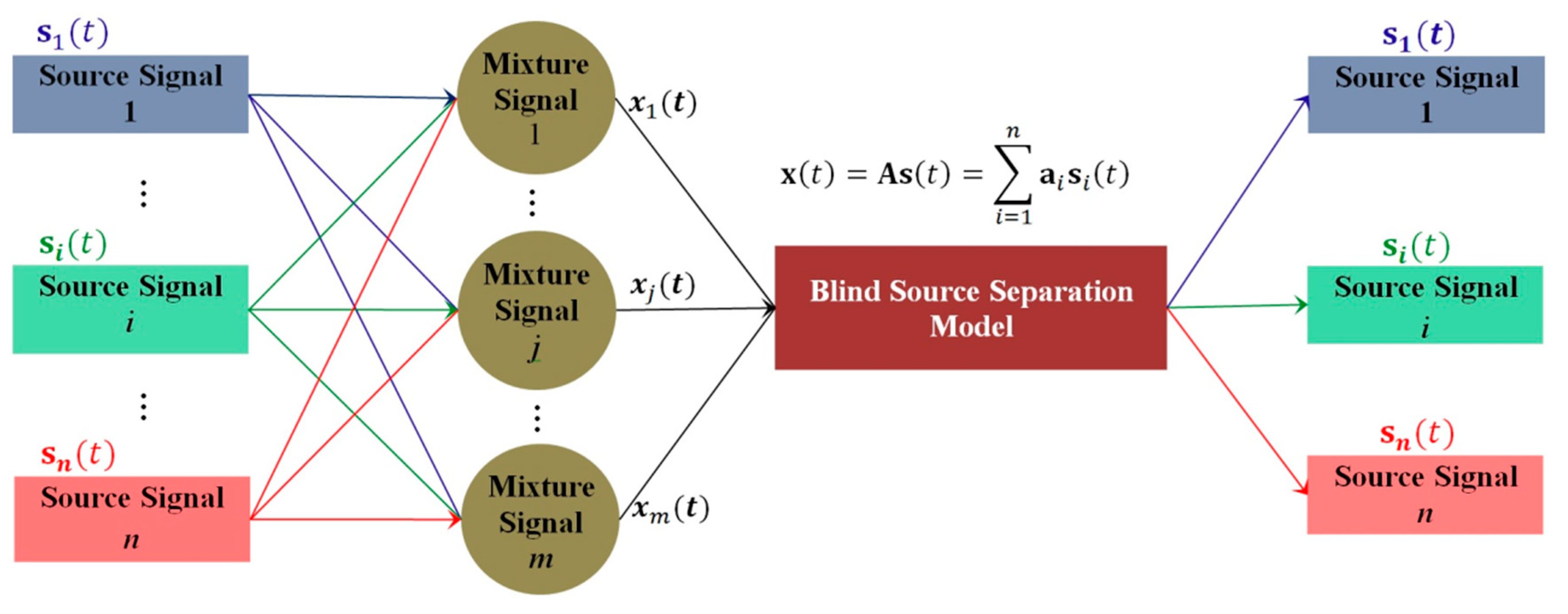
Recently, blind source separation (BSS) techniques have been used as promising signal analysis tools in various fields of science [12,13,14]. BSS based algorithms such as independent component analysis (ICA) [15] and second-order blind identification (SOBI) [16,17] are computational methods used for separating a multivariate signal into their individual subcomponents. These methods were applied in structural dynamics for the first time in Reference [18] to conduct output-only modal identification of structures. Furthermore, comparisons of the BSS based techniques and their limitations for modal analysis have been investigated in References [14,19,20,21]. BSS techniques are non-parametric data-driven algorithms, which extract modal features and perform structural assessment directly from the available data. BSS based methods are computationally efficient compared to the parametric methods that do not need a mathematical model to describe the physical performance of a system. Unlike parametric methods there is no need to adjust any parameter which keeps away the challenges like modal order problem [22]. Advances in blind source separation (BSS) techniques for modal identification and damage detection have offered novel opportunities to develop new data-driven methodologies for efficient and effective sensing and processing of large scale health monitoring data.

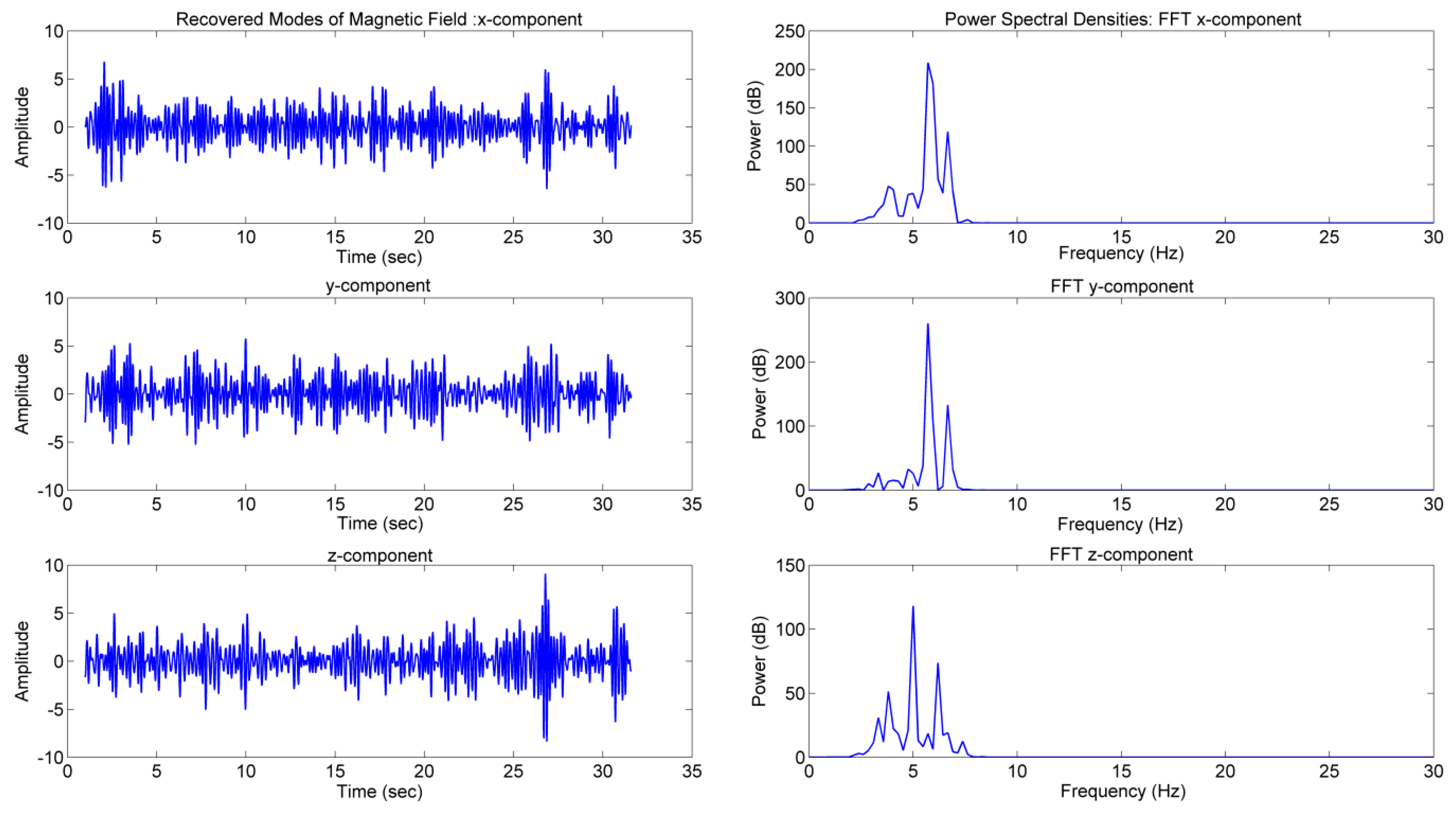
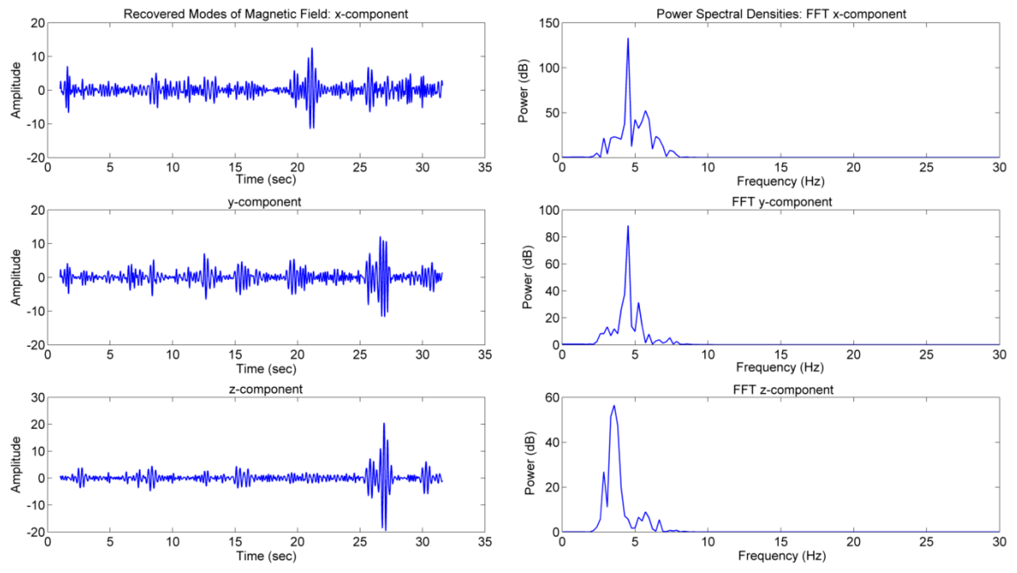
This study presents a time-domain output data identification model for pipeline magnetic field data using the unsupervised blind source separation technique termed complexity pursuit (CP) [23] that was independently formulated in Reference [24]. CP learning algorithms have been successfully applied for system identification and damage detection in References [22,25,26]. The main contribution of this paper is to apply the CP algorithms to the pipelines noisy magnetic field data, towards an accurate time-based modal identification. These non-parametric data driven algorithms has the ability to perform quick even real time, automatic sensing and processing of the large scale pipeline’s magnetic field data sets, that can provide excellent grounds for the inspection of buried ferromagnetic pipelines. The 3-axis magnetic field sensor data are fed as input into the blind source separation model where the complexity pursuit algorithms are applied for an accurate extraction of mode matrix that is then plotted to obtain the time-domain output modal responses. The frequency and damping ratio are computed from the recovered modal responses using Fourier transform and logarithm-decrement technique, respectively. The power spectral densities calculated from the recovered mode matrix show the abrupt variation in frequency due to the defects occurring in the pipeline. A numerical study for multi-degree of freedom systems and detailed indoor and outdoor experimental results show the ability of the non-parametric CP-BSS learning algorithms to accurately extract time-based modal information of the pipeline structures.

2. Blind Source Separation Problem

The process of identifying and extracting the original source signals from a mixture of signals with little information about the properties of the original source signals is termed as blind source separation.

The linear instantaneous blind source separation model is expressed as:

$$x\left(t\right)=As\left(t\right)={\displaystyle \sum }_{i=1}^n{a}_i{s}_i\left(t\right)$$

(1)

where $x\left(t\right)={\left[x_1\left(t\right),\dots ,x_m\left(t\right)\right]}^T$ is the measured signal, containing $m$ mixture signals, and $s\left(t\right)={\left[s_1\left(t\right),\dots ,s_n\left(t\right)\right]}^T$ is the original source vector with $n$ sources; $A\in R^{m\times n}$ is an unknown matrix consisting of n columns with its $i^{\mathrm{th}}$ column $a_i\in R^m$ associated with $s_i\left(t\right).$ Figure 1 shows a graphical interpretation of the blind source separation problem.

3. Stone’s Theorem for Solution of BSS Problem

Stone [23] proposed that under the effect of some physical laws, the moment of mass in a given time produces possible sources in a system. Likewise, the measured system responses also contains least complex sources, each source is created under the influence of certain physical law. Summarizing, the complexity of a mixture of response signals can be found among the simplest and the most composite constituent sources. This theory was proved in Reference [27].

This conclusion laid the foundation that source signals are the least complex signals that can be separated from the measured mixture of signals. Therefore, complexity pursuit algorithms search for source signals with least complexity, such that the “hidden” source component ${\mathit{z}}_i\left(\mathrm{t}\right)$ which is obtained by multiplying the mixture $x\left(\mathrm{t}\right)$ with the demixing row vector $w_i$ which is the least complex signal.

$${\mathit{z}}_i\left(t\right)=w_{i}x\left(t\right)$$

(2)

This approach has been used as a solution towards the BSS problem.

Stone [23] concluded that the complexity of a signal can be measured by maximizing the temporal predictability of a signal; the mathematical equation for temporal predictability is written by Reference [23] as:

$$F({\mathit{z}}_i)=\log \frac{V\left({\mathit{z}}_i\right)}{U\left({\mathit{z}}_i\right)}=\log \frac{{{\displaystyle \sum }}_{t=1}^N{\left(z_L\left(t\right)-{\mathit{z}}_i\left(t\right)\right)}^2}{{{\displaystyle \sum }}_{t=1}^N{\left({\mathit{z}}_S\left(t\right)-{\mathit{z}}_i\left(t\right)\right)}^2}$$

(3)

$F\left({\mathit{z}}_i\right)$ is the temporal predictability operator that contains the statistical and time-based information of the hidden source signal ${\mathit{z}}_i\left(t\right)$, that can be measured by finding the logarithmic ratio of $V\left({\mathit{z}}_i\right)/U\left({\mathit{z}}_i\right)$.

The term $V\left({\mathit{z}}_i\right)$ determines the global statistical information of signal ${\mathit{z}}_i\left(\mathrm{t}\right)$ by computing the ‘overall variability’, estimated by a long-range prediction ${\mathit{z}}_L\left(t\right)$. Similarly, $U\left({\mathit{z}}_i\right)$ determines the local variance that calculates the time-based information [23], using a short-range prediction parameter ${\mathit{z}}_S\left(t\right)$ on the temporal structure of ${\mathit{z}}_i\left(t\right)$. The filtration process is performed by the long range prediction parameter and short-range prediction parameter, mathematically expressed as,

$$\begin{gathered} {\mathrm{z}}_L\left(t\right)={\lambda }_L{z}_L\left(t-1\right)+\left(\left(1-{\mathsf{\lambda }}_L\right){\mathit{z}}_i\left(t-1\right)\right)0\le {\mathsf{\lambda }}_L\le 1 \\ {z}_S\left(t\right)={\mathsf{\lambda }}_S{z}_S\left(t-1\right)+\left(\left(1-{\mathsf{\lambda }}_S\right){\mathit{z}}_i\left(t-1\right)\right)0\le {\mathsf{\lambda }}_S\le 1 \end{gathered}$$

(4)

$\lambda =2^{-1/h}$ where $\mathrm{h}$ is termed as a half-life parameter for $h_S=1$ and $h_L=\mathrm{900,000}$ as long as $h_L\gg h_{\mathrm{S}},$ [23].

The significance of the proposed algorithm is to extract the hidden sources with accurate time-based structure. A careful selection of parameters is essential to predict a component with reduced local variance (smoothness) as compared with its global (long-range) variance, as the increase of the global statistical information $V\left({\mathit{z}}_i\right)$ only will produce a high variance signal, while increasing $U\left({\mathit{z}}_i\right)$ only will produce a smooth DC signal.

4. System Identification by CP

Combining Equation (2) and Equation (3)

$$F({\mathit{z}}_i)=F(w_i,x)=\log \frac{V(w_i,x)}{U(w_i,x)}=\log \frac{w_i\overline{P}{w}_i^T}{w_i\widehat{P}{w}_i^T}$$

(5)

where $\overline{P}$ and $\widehat{P}$ are the $M\mathrm{x}M$ short-range and long-range covariance matrices among the mixtures, respectively. The elements of these matrices are given by

$$\begin{gathered} {\widehat{p}}_{ij}={\displaystyle \sum }_{t=1}^N\left(p_i\left(t\right)-{\widehat{p}}_i\left(t\right)\right)\left(p_j\left(t\right)-{\widehat{p}}_j\left(t\right)\right) \\ {\overline{p}}_{ij}={\displaystyle \sum }_{t=1}^N\left(p_i\left(t\right)-{\overline{p}}_i\left(t\right)\right)\left(p_j\left(t\right)-{\overline{p}}_j\left(t\right)\right) \end{gathered}$$

(6)

The matrices $\overline{P}$ and $\widehat{P}$ are calculated only once and the terms $\left(p_i\left(t\right)-{\widehat{p}}_i\left(t\right)\right)$ and $\left(p_j\left(t\right)-{\overline{p}}_j\left(t\right)\right)$ are calculated by fast convolution operations. For a given mixture of signals $x\left(t\right)$, the complexity pursuit algorithm calculates the de-mixing vector $w_i$ by maximizing the temporal predictability function $F({\mathit{z}}_i)$;

The derivative of $F$ with respect to $w_i$ is given by

$${\nabla }_{w_i}F=\frac{2w_i}{V_i}\overline{P}-\frac{2w_i}{U_i}\widehat{P}$$

(7)

Using the gradient ascent technique a maximum value of $F$ can be obtained by repeatedly updating $w_i;$ such that the extracted component $z_i=w_{i}x$, which is “most predictable” is considered as the least complex signal or the simplest source hidden in the mixtures [23].

Considering the uncertainties of the proposed CP model for extracting only one simplest source can be solved by the deflation scheme [22]. The sources are simultaneously extracted one after another using Gram–Schmidt de-correlation technique. The first step is to separate the most simplest source present in the mixture, after removing the first source the currently simplest source becomes the second one to be separated by the complexity pursuit algorithm and so on. The solution for gradient of $F$ approaches zero such that,

$${\nabla }_{w_i}F=\frac{2w_i}{V_i}\overline{P}-\frac{2w_i}{U_i}\widehat{P}=0$$

(8)

Rearranging Equation (8)

$$w_i\overline{P}=\frac{V_i}{U_i}{w}_i\widehat{P}$$

(9)

Equation (9) has the form of a generalized eigenproblem; $w_i$ can be found as the eigenvectors of matrix ${\widehat{P}}^{-1}\overline{P}$, with corresponding eigenvalue $s {\mathsf{\gamma }}_i=V_i/U_i$, [23]. The de-mixing matrix $A=W^{-1}$ is calculated using a generalized eigenvalue routine. All the source signals can be separated by:

$$s\left(t\right)=\mathit{z}\left(t\right)=Wx\left(t\right)$$

(10)

$s\left(t\right)={[{\mathit{s}}_1\left(t\right),\dots .,{\mathit{s}}_n\left(t\right)]}^T$ is the recovered source matrix with row-wise source signals $s_i\left(t\right)$.

5. Modal Parameters Estimated by CP

The governing equation of motion for a linear time invariant system is given by

$$M\ddot{x}+C\dot{x}\left(t\right)+Kx\left(t\right)=f\left(t\right)$$

(11)

where $M$ is mass, $C$ is damping matrix and $K$ is the stiffness matrix, all real valued and symmetric. $x\left(t\right)$ is the displacement vector, which are actually the measured system responses. $f\left(t\right)$ is the external force acting on the system.

The connection of blind source separation with output modal identification was solved for the first time in Reference [18], as in the BSS model in Equation (1), the modes of a system can be expanded as a linear combination of n number of modal responses: that can be expressed in Equation (12) as:

$$x\left(t\right)=\Phi q\left(t\right)={\displaystyle \sum }_{i=1}^{\mathrm{n}}{\mathit{\phi }}_i{\mathit{q}}_i\left(t\right)$$

(12)

The basic phenomenon of Equation (12) is same as in Equation (1), Φ contains the modal information of a system describing the entire situation of a noise contaminated system. ${\phi }_i\in {ℝ}^n$ being the (mode shape) is related to the ith modal feature column of the mode matrix, and is related with the ith modal response $q_i\left(t\right)$ of the modal response vector $q\left(t\right)$. $q\left(t\right)$ is actually the original source signal that can be obtained by multiplying the inverse of the mode matrix with the $\left(m\mathrm{x}n\right)$ matrix of the measured system responses.

$$q\left(t\right)={\Phi }^{-1}x\left(t\right)$$

(13)

$\Phi \in {ℝ}^{nxn}$ is used to identify the change in the normal condition of a system as an abrupt variation in the modal feature. Therefore, plotting the mode shapes can give important information about the damage occurring in the system under observation.

The idea of “virtual sources” in Reference [18] states that the recovered modal responses of a system should be considered as independent sources, if the power spectral density is not same or the frequencies are not able to be judged clearly. In such cases the mixing matrix matches with the recovered modal matrix, consequently the hidden sources and unidentified mixing matrix can be obtained by putting the measured system responses from the expanded model in Equation (12) as known mixtures into the blind source separation framework in Equation (1); accordingly the desired modal responses and mode matrix can be achieved.

Equation (12) can be used to classify the motion of a system by its mode matrix $\Phi$ as it provides complete information about the linear system. Putting Equation (12) into Equation (11) and multiplying the transpose of the mode matrix ${\Phi }^T$ on both sides,

$${\Phi }^{T}M\Phi \ddot{q}\left(t\right)+{\Phi }^{T}C\Phi \dot{q}\left(t\right)+{\Phi }^{T}K\Phi q\left(t\right)={\Phi }^{T}f\left(t\right)$$

(14)

yields to

$$M^{*}\ddot{q}\left(t\right)+C^{*}\dot{q}\left(t\right)+K^{*}q\left(t\right)=f^{*}\left(t\right)$$

(15)

where $M^{*}$ is the diagonal real-valued modal mass matrix, $C^{*}$ is the damping matrix, and $K^{*}$ is the stiffness matrix. $f^{*}\left(t\right)$ is the modal force vector. A multi-DOF system can be decoupled into n-DOF systems whose motions are given by

$${\mathit{m}}_i^{*}{\ddot{\mathit{q}}}_i\left(t\right)+{\mathit{c}}_i^{*}{\dot{\mathit{q}}}_i\left(t\right)+{\mathit{k}}_i^{*}{\mathit{q}}_i\left(t\right)={\mathit{f}}_i^{*}\left(t\right)$$

(16)

Equation (16) defines the basic idea of the complexity pursuit algorithm by targeting the motion of the decoupled single degree of freedom system on ith modal coordinate ${\mathit{q}}_i\left(t\right)$. The modal parameters of the system i.e. damping ratio is calculated by ${\varsigma }_i={\mathit{c}}_i^{*}/2\sqrt{{\mathit{m}}_i^{*}{\mathit{k}}_i^{*}}$ and resonant frequency of the system is calculated in terms of natural frequency ${\omega }_i$ of the ith mode given by ${\omega }_{di}={\omega }_i\sqrt{1-{\varsigma }_i^2}=\sqrt{\left(1-{\varsigma }_i^2\right){\mathit{k}}_i^{*}/{\mathit{m}}_i^{*}}$.

In free excitation, i.e., $f\left(t\right)=0$, the modal responses behave like exponentially decaying sinusoids. The motion of mass at ith modal coordinate governed by Equation (16) can be written as

$${\mathit{q}}_i\left(t\right)=u_i{e}^{-{\varsigma }_i{\omega }_{i}t}\cos \left({\omega }_{di}t+{\theta }_i\right)$$

(17)

The measured mixtures are linear combinations of these modal responses, written as

$$x\left(t\right)=\Phi q\left(t\right)={\displaystyle \sum }_{i=1}^n{\mathit{\phi }}_i{\mathit{q}}_i\left(t\right)={\displaystyle \sum }_{i=1}^n{\mathit{\phi }}_i{u}_i{e}^{-{\varsigma }_i{\omega }_{i}t}\cos \left({\omega }_{di}t+{\theta }_i\right)$$

(18)

where $u_i$ and ${\theta }_i$ are some constants determined by initial conditions.

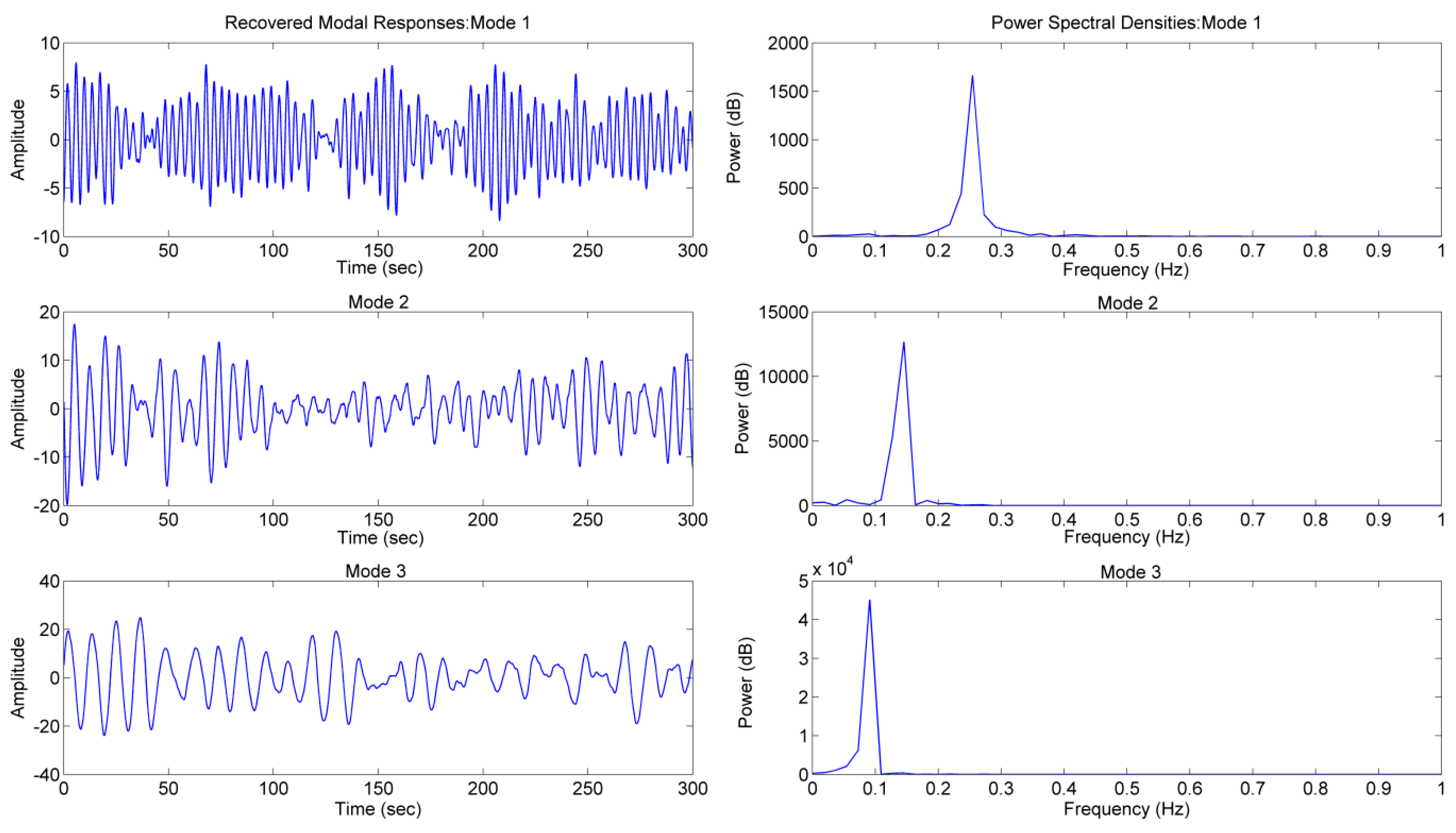
In case of random excitation, the recovered modal responses are dominant over the measured system response, producing randomly modulated exponentially decaying sinusoids with an envelope function $e_i\left(t\right)$ at the ith mode [18],

$${\mathit{q}}_i\left(t\right)\cong e_i\left(t\right)u_i{e}^{-{\varsigma }_i{\omega }_{i}t}\cos \left({\omega }_{di}t+{\theta }_i\right)$$

(19)

Hence, the measured responses are given by

$$x\left(t\right)={\displaystyle \sum }_{\mathrm{i}=1}^{\mathrm{n}}{\mathit{\phi }}_i{q}_i\left(t\right)\cong {\displaystyle \sum }_{\mathrm{i}=1}^{\mathrm{n}}{\mathit{\phi }}_i{e}_i\left(t\right)u_i{e}^{-{\varsigma }_i{\omega }_{i}t}\cos \left({\omega }_{di}t+{\theta }_i\right)$$

(20)

In case of highly damped systems with complex valued mode matrix the complexity pursuit algorithms can separate the system into their respective modes until the intrinsic frequency and damping property of the system does not change. In such case the physical system in Equation (12) can be decoupled into Equation (17) in the state-space by the excitation mode matrix ${\Phi }_c$, as well as the modal responses $q_c\left(t\right)$. Therefore, using Stone’s algorithm the measured mixture $x\left(t\right)$ consisting of time based modal responses $q\left(t\right),$ can be subsequently separated by CP–BSS model,

$$\tilde{q}\left(t\right)=s\left(t\right)=Wx\left(t\right)$$

(21)

and the excitation mode matrix can be estimated by

$$\tilde{\Phi }=W^{-1}$$

(22)

The frequency and damping ratio can be readily computed from the recovered time-domain modal response $\tilde{q}\left(t\right)$ using Fourier transform and logarithm-decrement technique, respectively. Yang and Nagarajaiah [22] solved the modal order problem in complexity pursuit based blind source separation method by arranging the recovered modes ordering the frequency values, i.e., the first mode can be identified by the modal response with smallest frequency and so on.

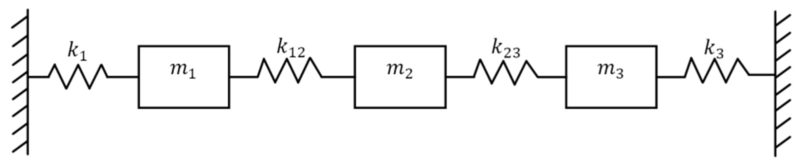
6. Numerical Simulations

Using the CP based BSS algorithm, numerical examples are conducted on a 3-DOF system shown in Figure 2 including different levels of damping.

The system parameters are adjusted to classify different modal identification problems i.e. proportional damping well-separated mode, closely spaced mode and complex mode. Free excitation and random excitation in each case are discussed. Gaussian White Noise (GWN) is used to produce stationary random excitation. Similarly the Gaussian White Noise (GWN) is modulated with a constant exponential decay function to create a non-stationary excitation effect in the system. The time histories of the system responses, i.e., the displacement vector, are calculated by the Newmark-Beta solver. The sampling frequency is set to 10 Hz.

The parameters of complexity pursuit based blind source separation method remains the same throughout the process. The long-range parameter $h_L$ = 900,000 and short-range parameter $h_S$ = 1 are taken same as given by Reference [23]. Fast convolution operations are performed to calculate the long-range and short-range covariance matrices. The demixing matrix which is the eigenvector matrix is calculated by conducting eigenvalue decomposition on the obtained covariance matrices. The excitation mode matrix and the time-domain modal responses are calculated by Equations (21) and (22) respectively. Fourier transform algorithms and logarithm-decrement technique are used to calculate frequency and damping ratio respectively.

A modal assurance criterion is defined in Equation (23) to evaluate the correlation among the recovered mode values ${\tilde{\phi }}_i$ and the theoretical mode values ${\phi }_i,$

$$\mathrm{MAC}\left({\tilde{\phi }}_i,{\phi }_i\right)=\frac{{\left({\tilde{\phi }}_i^T,{\phi }_i\right)}^2}{\left({\tilde{\phi }}_i^T.{\tilde{\phi }}_i\right)\left({\phi }_i^T.{\phi }_i\right)}$$

(23)

Ranging from 0 to 1, where 0 means no correlation and 1 indicates perfect correlation.

6.1. Proportional Damping

The parameters of the system shown in Figure 2 are borrowed from Reference [18]. In case of proportional damping

$$\mathbf{M}=\left[\begin{array}{ccc}2& 0& 0\\ 0& 1& 0\\ 0& 0& 3\end{array}\right]\mathbf{K}=\left[\begin{array}{ccc}2& -1& 0\\ -1& 2& -1\\ 0& -1& 2\end{array}\right]\mathbf{C}=\alpha \mathbf{M}=\alpha \left[\begin{array}{ccc}2& 0& 0\\ 0& 1& 0\\ 0& 0& 3\end{array}\right]$$

$M$ is the mass matrix, $K$ is the stiffness matrix and $C$ is the damping matrix. The value of $\alpha$ corresponds to different damping level, ($\alpha =0.08$ and $0.13$). $\mathrm{f}\left(t\right)=0$ in free excitation with initial condition $\mathrm{x}\left(0\right)={\left[\begin{array}{ccc}0& 1& 0\end{array}\right]}^T$ and $\dot{\mathrm{x}}\left(0\right)={\left[\begin{array}{ccc}0& 0& 1\end{array}\right]}^T$. In case of random excitation the system is excited at the 2nd and 3rd DOFs using stationary and non-stationary Gaussian white noise.

Table 1. Identified modal parameters (proportional damping).

Mode	Comparison	Frequency (Hz)			Damping Ratio (%)
		1	2	3	1	2	3
α = 0.08	Theoretical Value	0.0895	0.1458	0.2522	4.4437	2.7299	1.5775
	CP Identified Value	0.0879	0.1465	0.2539	4.4493	2.8233	1.5248
α = 0.13	Theoretical Value	0.0895	0.1458	0.2522	11.5537	7.0977	4.1015
	CP Identified Value	0.0879	0.1465	0.2539	11.4167	7.3448	3.9240

and

Table 2. Identified Modal Assurance Criteria values (proportional damping).

α	Free Excitation			Stationary GWN			Non-Stationary GWN
Mode	1	2	3	1	2	3	1	2	3
0.08	0.9975	0.9993	0.9990	1.0000	0.9962	0.9998	0.9998	0.9977	0.9981
0.13	0.9929	0.9816	0.9876	0.9990	0.9916	0.9996	0.9996	0.9977	0.9873

show the obtained results by CP algorithms and the modal assurance criterion values respectively.

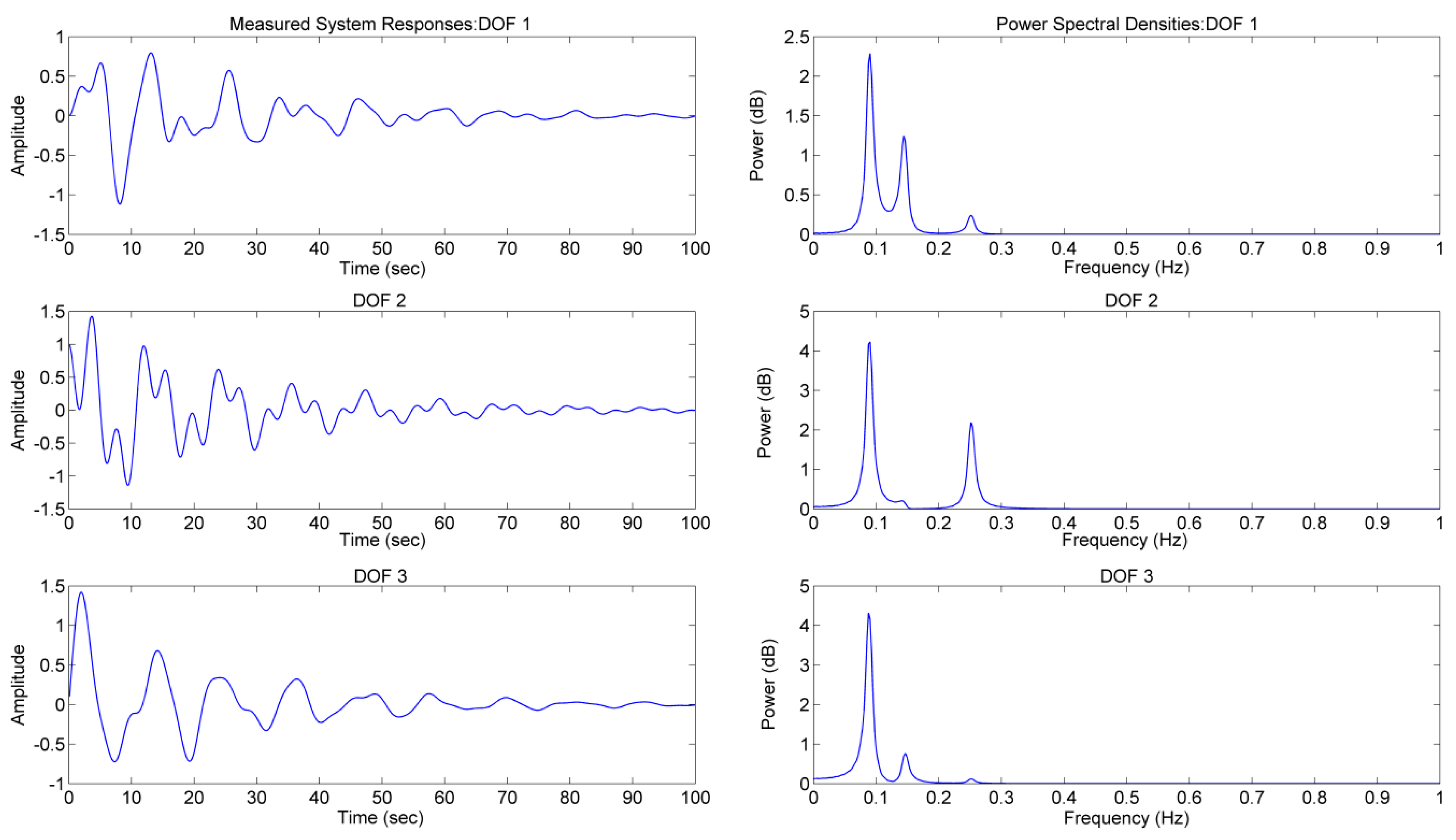
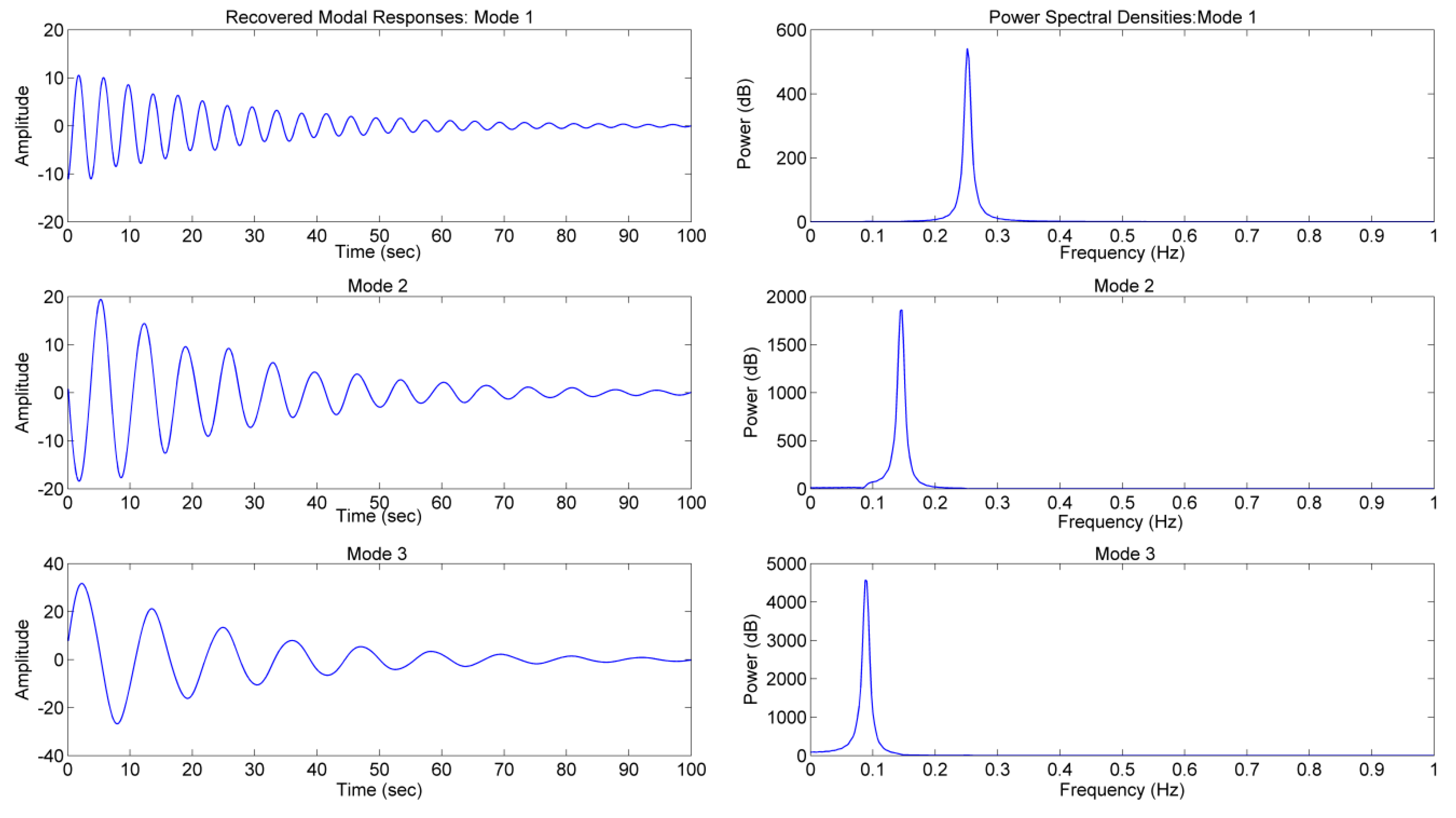
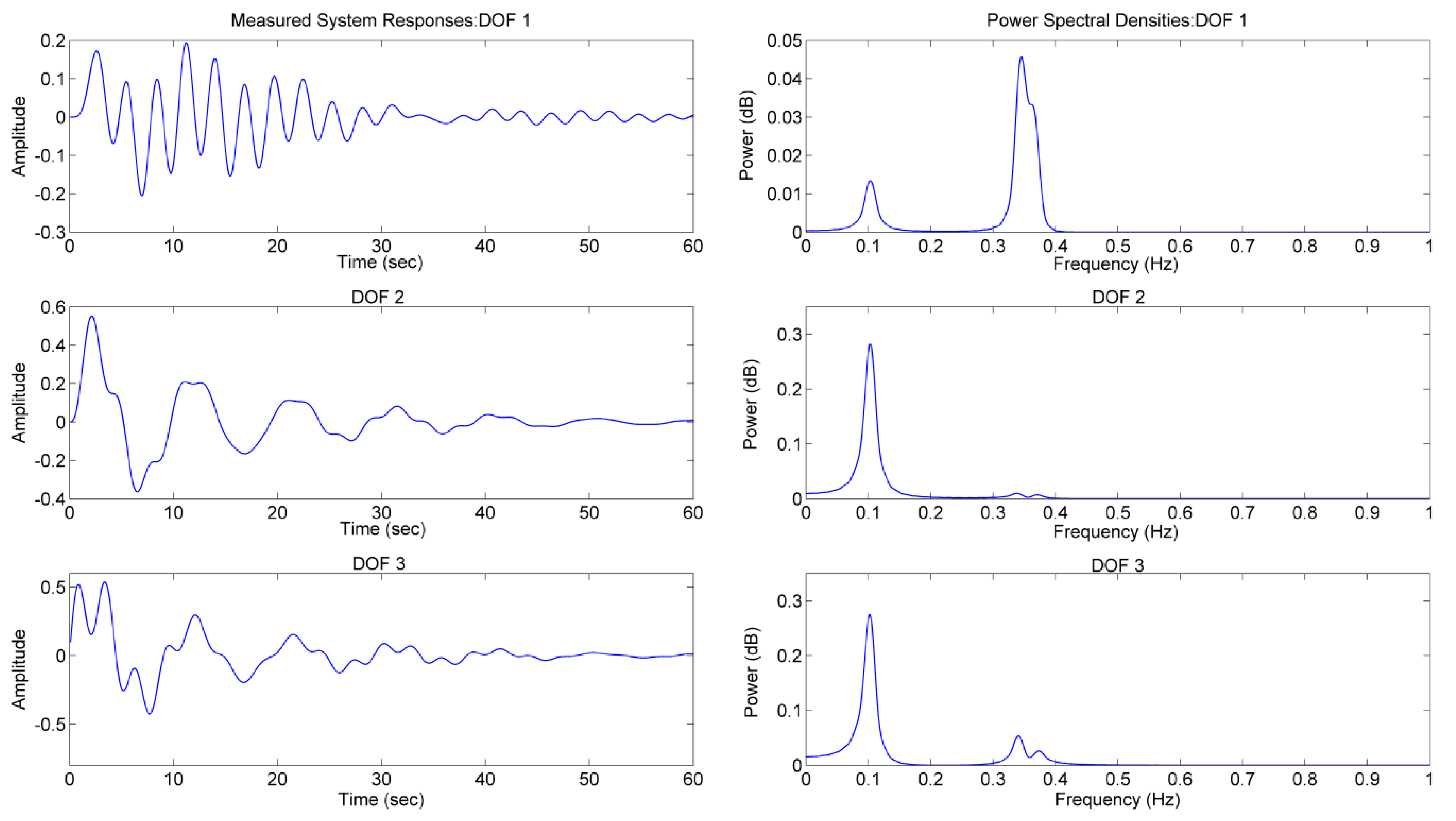
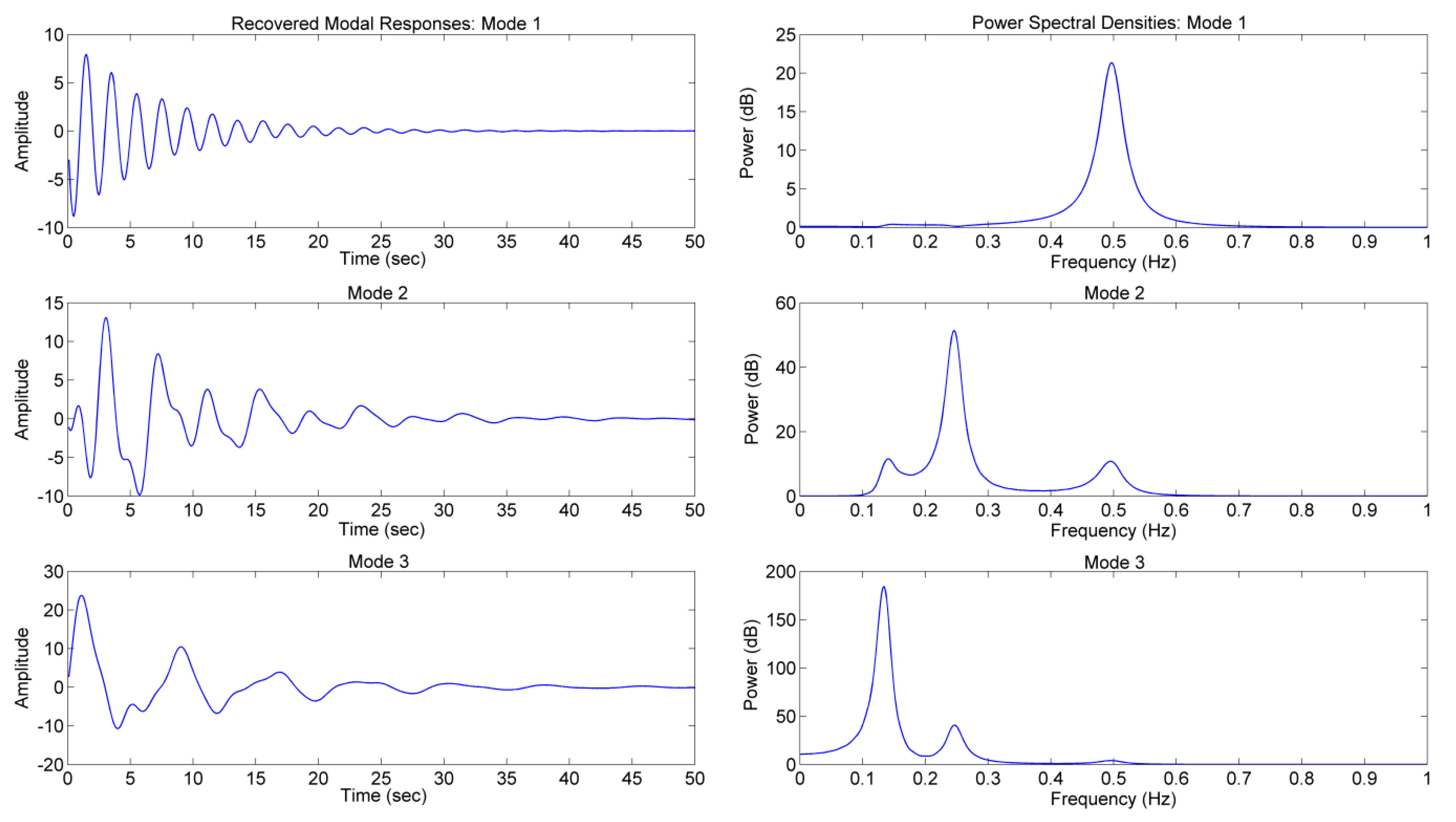
Figure 3 shows the measured responses of a 3DOF linear system for $\mathsf{\alpha }=0.08$ in free excitation proportional damping. After applying CP-BSS the estimated modes in free excitation are given in Figure 4 and Figure 5, respectively. The order of the recovered modal responses in each case is not rearranged to show the original results by CP model; (for example the Mode 1 in Figure 4 simply means the first mode recovered by CP algorithm, not suggesting Mode #1). This is due to modal order problem that can be solved by rearranging the frequency values. Thus it can be observed that the measured responses of the 3DOF system are well-separated into their respective modes. The frequency of the separated modes can be observed from the power spectral densities of the estimated modes.

6.2. Effect of Noise

The calculated signal responses are now contaminated by adding zero-mean Gaussian white noise (with a 10% of the original signal). The results for $\mathsf{\alpha }=0.08$ in free excitation are shown in

Table 3. Identification results by CP in 10% root-mean-square noise ($\mathsf{\alpha }=0.08$).

Mode	Frequency (Hz)		Damping Ratio (%)		MAC Values
	Theoretical Value	CP Identified	Theoretical Value	CP Identified
1	0.0894	0.0885	4.4437	4.2151	0.9989
2	0.1457	0.1459	2.7299	2.7910	0.9617
3	0.2521	0.2529	1.5775	1.5343	0.9979

, addition of noise has no influence on the output of the CP model. The same accuracy has been seen in cases with various damping levels. This means that the CP algorithm provides healthy outputs for noise added signals also.

6.3. Closely Spaced Modes

The complexity pursuit model was implemented on measured system responses of a 3DOF system with closely spaced modes. The mass, stiffness and damping matrix were obtained by modifying the high proportional damping matrix in Reference [21],

$$\mathrm{M}=\left[\begin{array}{ccc}1& 0& 0\\ 0& 2& 0\\ 0& 0& 1\end{array}\right]\mathrm{K}=\left[\begin{array}{ccc}5& -1& 0\\ -1& 4& -3\\ 0& -3& 3.5\end{array}\right]\mathrm{C}=\mathsf{\alpha }\mathrm{M}=\mathsf{\alpha }\left[\begin{array}{ccc}1& 0& 0\\ 0& 2& 0\\ 0& 0& 1\end{array}\right]$$

The initial conditions used in free excitation are changed to $\mathrm{x}\left(0\right)={\left[\begin{array}{ccc}0& 0& 0\end{array}\right]}^T$ and $\dot{\mathrm{x}}\left(0\right)={\left[\begin{array}{ccc}0& 0& 0\end{array}\right]}^T$, the remaining parameters were left the same as used in proportional damping case. Fairly accurate modal identification results are obtained in closely spaced modes shown in

Table 4. Identification results of free excitation in closely spaced modes cases.

Mode	Comparison	Frequency (Hz)			Damping Ratio (%)
		1	2	3	1	2	3
α = 0.08	Theoretical Value	0.1039	0.3425	0.3713	3.8279	1.1618	1.0715
	CP Identified Value	0.1074	0.3418	0.3711	3.8199	1.1434	1.0151
α = 0.13	Theoretical Value	0.1039	0.3425	0.3713	9.9526	3.0208	2.7860
	CP Identified Value	0.1074	0.3418	0.3711	9.9770	2.9906	2.7274

and

Table 5. Modal assurance criterion results in closely space mode cases.

α	Free Excitation			Stationary Gaussian White Noise			Non-Stationary Gaussian White Noise
Mode	1	2	3	1	2	3	1	2	3
0.08	1.0000	0.9971	0.9999	0.9999	1.0000	0.9991	1.0000	0.9973	0.9963
0.13	1.0000	0.9735	0.9759	0.9998	0.9999	1.0000	0.9999	0.9765	0.9914

, respectively.

A highly damped system $\left(\alpha =0.13\right)$ with closely spaced mode in free excitation is shown in Figure 6. The closely spaced 2nd and 3rd modes of the system responses that can be hardly judged in the power spectral densities are clearly decoupled by the CP model as shown in Figure 7.

6.4. Non-Proportional Damping

The parameters of a system under non-proportional damping are given as follows,

$$\mathrm{M}=\left[\begin{array}{ccc}3& 0& 0\\ 0& 2& 0\\ 0& 0& 1\end{array}\right]\mathrm{K}=\left[\begin{array}{ccc}4& -2& 0\\ -2& 4& -2\\ 0& -2& 10\end{array}\right]\mathrm{C}=\left[\begin{array}{ccc}0.3856& 0.2290& -0.9702\\ 0.2290& 0.5080& -0.0297\\ -0.9702& -0.0297& 0.3241\end{array}\right]$$

The model was obtained by slightly changing the damping matrix used in Reference [21] that results in complex modes. McNeil and Zimmerman [21] presented a standard method to transform the complex modes into real ones due to the output of the complexity pursuit model to provide a real value demixing matrix.

Table 6. Identified results of free excitation in non-proportional high damping.

Mode	Frequency (Hz)		Damping Ratio (%)		Modal Assurance Criterion
	Identified	Theoretical	Identified	Theoretical
1	0.1377	0.1353	10.959	10.889	0.9853
2	0.2391	0.2444	6.7317	6.8753	0.9520
3	0.4970	0.5084	4.6748	4.8727	0.9813

and

Table 7. Identified MAC values for non-proportional high damping.

α	Free Excitation			Stationary Gaussian White Noise			Non-Stationary Gaussian White Noise
Mode	1	2	3	1	2	3	1	2	3
0.01	1.0000	0.9999	0.9998	0.9999	1.0000	0.9996	1.0000	1.0000	0.9990
0.05	1.0000	0.9971	0.9999	0.9999	1.0000	0.9991	1.0000	0.9973	0.9963
0.13	1.0000	0.9735	0.9759	0.9998	0.9999	1.0000	0.9999	0.9765	0.9914

show the identification results. Fairly well comparison can be seen among the identified and the theoretical results. Equation (23) can be used to evaluate the accuracy of the identified mode shapes. The system responses and recovered modal responses are shown in Figure 8 and Figure 9, respectively. Little influence on the output of the CP algorithm has been seen in case of non-proportional damping; still it offers better approximation compared to the theoretical values for complex modes.

6.5. Modal Identification of a 12-DOF System

The performance of complexity pursuit algorithms is further extended towards large scale structures, a 12-DOF system is built up such that the values of constant mass matrix $M$ are given by; ${\mathrm{m}}_1=2$, ${\mathrm{m}}_2\dots ,{\mathrm{m}}_{11}=1$, ${\mathrm{m}}_{12}=3,$ and values of stiffness matrix $\mathrm{K}$ are ${\mathrm{k}}_1,{\mathrm{k}}_2,\dots {\mathrm{k}}_{13}=20000$ and damping matrix is calculated by $\mathrm{C}=\mathsf{\alpha }\mathrm{M}$ with $\alpha =3,$ where $\alpha$ is the damping ratio. The first mode has a theoretical damping ratio of 4.46%. The frequencies of the 12 modes are distributed between 5.3505 and 44.5827 Hz; with a sampling frequency set to 1000 Hz. The system is excited at the 12th DOF, and the time histories of the signals with 5000 samples are measured (the length of the signal can be increased and the accuracy holds). Modal assurance criterion (MAC) values for all 12 modes under different conditions are shown in

Table 8. MAC values for 12-DOF System Proportional Damping.

Modes	Free Excitation			Stationary GWN			Non-Stationary GWN
	α = 1	α = 2	α = 3	α = 1	α = 2	α = 3	α = 1	α = 2	α = 3
1	0.9950	0.9972	0.9904	0.9989	0.9946	0.9837	0.9973	0.9975	0.9938
2	0.9974	0.9977	0.9939	0.9989	0.9951	0.9857	0.9970	0.9979	1.0000
3	0.9994	0.9952	0.9922	0.9982	0.9981	0.9937	0.9989	0.9948	0.9921
4	0.9997	0.9977	0.9959	0.9995	0.9982	0.9927	0.9996	0.9974	0.9958
5	0.9999	0.9992	0.9985	0.9999	0.9995	0.9991	0.9998	0.9991	0.9985
6	0.9998	0.9997	0.9995	0.9999	0.9996	0.9996	0.9998	0.9997	0.9995
7	0.9999	0.9998	0.9997	1.0000	0.9998	0.9997	0.9999	0.9998	0.9997
8	1.0000	0.9999	0.9999	1.0000	1.0000	0.9999	1.0000	0.9999	0.9999
9	1.0000	1.0000	1.0000	1.0000	1.0000	1.0000	1.0000	1.0000	1.0000
10	1.0000	1.0000	0.9999	1.0000	1.0000	0.9999	1.0000	1.0000	0.9999
11	1.0000	1.0000	0.9999	1.0000	1.0000	0.9999	1.0000	1.0000	0.9999
12	1.0000	1.0000	0.9999	1.0000	1.0000	0.9999	1.0000	1.0000	0.9999

. A high correlation among the approximated modes can be seen with (MAC) values above 0.99 for all damping levels.

7. Experimental Analysis

7.1. Measurement Probe Designed to Detect the Magnetic Field of a Pipeline Based on the Principles of Magnetic Gradient Tensor

The block diagram of the complete measurement system is shown in Figure 10a. It consists of batteries, magnetic probe, National Instruments data acquisition system, industrial control computers, and a global positioning system. Two rechargeable batteries (24 V and 12 V) are connected as power source to all the measurement system. A global positioning system (GPS) is used to locate the position of a buried pipeline at each point of the measured distance. The measurement array of magnetic probe is composed of five triaxial magnetic field sensors shown in Figure 10b. The sensor to sensor baseline distance $d$ is 0.1 m. The analog signals collected by each sensor are comprised of x, y and z-components of the magnetic field. The measured signals are converted into digital data by the National Data Acquisition System. This digital data is further transferred to an industrial control computer. This part of measurement system is the computer (CPU) and a storage unit that records the real-time data to be used for further processing. A complete measurement system is shown in Figure 10c.

7.2. Indoor Data Recording Procedure

For indoor experiments a two-story robot was designed shown in Figure 11a. The magnetic probe is fixed at the first floor with sensors facing towards the pipeline. The National Instruments data acquisition units have been fixed at the second story above the magnetic probe. The robot is moved along the surface of the pipeline with a measurement length of 10 m. The pipeline test sample is made of Q235 steel with an inner wall to wall diameter of 0.1 m and wall thickness of 0.002 m. The height of the sensor probe from the pipeline is 1 m with a sampling frequency of 1 kHz. The defects on the wall of the pipeline can be seen in Figure 11b, i.e., a groove of depth 0.001 m and a hole of diameter 0.01 m at a distance of 4 m from each other. The measurement system data are arranged in a $m\mathrm{x}n$ matrix, with $m=15$ signals and $n=\mathrm{120,000}$ samples.

7.3. Indoor Experimental Results

The CP-BSS method is then applied on the measured data matrix. The recovered modal responses for x, y and z-components of magnetic field for Sensor 1 and Sensor 3 are given in Figure 12 and Figure 13, respectively. The results clearly indicate that the measured system data are accurately transformed into their respective modal responses. The power spectral densities calculated from the recovered mode matrix clearly shows the abrupt variation in power of the signal at given frequencies, i.e., 25 Hz and 75 Hz in all three power spectral densities which is due to the damage occurring in the pipeline, i.e., groove and hole present in the pipeline test sample.

7.4. Outdoor Data Recording Procedure

An outdoor experiment has been performed on an underground pipeline in Hebei province of China. The measurement setup shown in Figure 10c has been used to record the magnetic field data of the pipeline. A schematic illustration of the measurement procedure is shown in Figure 14. The pipeline is made from Q235 steel with a diameter $D=0.323\mathrm{m}$ and a wall thickness of $\delta =0.005\mathrm{m}$. The distance from the top of the pipeline to the ground is $h_1=0.5\mathrm{m}$, while the distance from the measurement plane to the ground is $h_2=1\mathrm{m}$. The sampling frequency is 100 Hz. $B_x$, $B_y$ and $B_z$ are the x, y and z components of the magnetic field of the pipeline respectively. The length of the pipeline is 16 m, for which the data signal has been recorded with a time history of 35 seconds.

7.5. Outdoor Experimental Results

The recovered modal responses for Sensors 1 and 3, along with their respective power spectral densities, are shown in Figure 15 and Figure 16, respectively. The identified visible modes are shown as the active modes present in the pipelines structural response data. The power spectral densities calculated from the recovered modes clearly reveals an abrupt variation in power of the source signals at given frequencies due to the damage occurring in the pipeline. The results demonstrate that the active modes present in the pipeline magnetic field can be accurately identified using the complexity pursuit based blind identification model.

8. Concluding Remarks

Time-domain output-only modal identification using novel blind source separation technique complexity pursuit was discussed in this paper. An application to the pipeline flaw detection is presented. A Complexity Pursuit algorithm is implemented for the blind identification of structural damage from the measured magnetic field data of a pipeline. Using Fourier transform the power spectral densities are calculated from the approximated modal responses. Numerical simulations for multi-DOF systems are carried out to explain and validate the CP based BSS method for proportional damping (well-separated and closely spaced modes) and non-proportional damping (complex modes) structures. The complexity pursuit based BSS model is implemented on the indoor and outdoor experimental data comprised of 3-axis magnetic field signals; it offers excellent results about the pipeline structural information. The process needs much less user interaction because the parameters of the model remain the same throughout the process of targeting the input data. Similarly the length of measured data does not influence the accuracy of the CP model. The performance of the unsupervised CP-BSS model to identify structural information makes it more suitable for real-time, as well as for off-line, inspection of pipeline structures.