A Semi-Automated Image-Based Method for Interfacial Roughness Measurement Applied to Metal/Oxide Interfaces

Abstract

Measuring interfacial roughness is essential in evaluating the adhesion of coatings and thermally grown oxides. Conventional contact methods are often impractical for such analyses, especially when the interface lies beneath a nonremovable layer. This study proposes a semi-automated method combining an ImageJ macro and an R-language script to assess interfacial roughness from images obtained through scanning electron microscopy (SEM), leveraging chemical contrast between substrate and oxide. The approach preserves user input where interpretation is critical while standardizing measurement to reduce variability. Applied to 21 images from seven experimental conditions, the algorithm successfully reproduced the roughness ranking obtained from manual measurement while also significantly reducing measurement dispersion. Though it underestimates absolute roughness values compared with the user measurements (which should also happen with conventional contact methods), it offers a robust, flexible, and reproducible alternative for interface characterization.

1. Introduction

Surface roughness is an important parameter in the evaluation of potential practical applications for new materials and fabrication processes, affecting tribological behavior, adhesive properties, and stress distribution, for example. Usually, quantitative methods for measuring roughness are based on direct exposure of the surface to the measuring device (contact methods), as is the case with mechanical probe instruments or optical sensors [1]. Some processes, however, require that the surface of the sample be covered with a different material. This can be done purposefully by the researcher, as is the case in the study of protective layers applied over a given substrate [2,3,4,5], or can be a direct consequence of the process, as is the case with oxidation studies of metallic alloys, which end with the growth of an oxide layer over the surface of the sample [6,7]. In both cases, the original surface of the sample is now an interface between its substrate and the film covering it, which renders the straightforward use of conventional roughness measurement techniques impossible.

This interfacial roughness, however, is a very important parameter, which was shown to have an effect on the adhesion between the substrate and protective films [8,9,10], for instance. In oxidation, the surface roughness has a significant effect on the oxide growth and adhesion [11,12,13,14]. These are often related to the initial surface roughness, which can be evaluated with conventional methods, but previous studies have shown that the oxidation process has a significant effect on interface roughness. The increase of the metal–oxide interface roughness during cyclic oxidation of FeMnSiCrNi alloys, for example, increased adhesion between the metallic substrate and the oxide [15,16,17]. While these interfaces can be observed by sectioning samples and subjecting them to analysis in a microscope, this method does not give a quantitative measure of the interfacial roughness. Computational simulations can be a solution in some cases, such as in the evaluation of stress distributions on the interface [15,18,19]. However, those are more fit to cases in which the effect of the interface roughness is unknown, but the roughness itself is known or can be estimated, for example, with mathematical equations [20,21], allowing the interface to be modeled.

Some successful attempts at a qualitative measuring technique via digital analysis of Scanning Electron Microscopy (SEM) images were reported previously [22,23,24,25]. The type of analysis presented by Carim and Sinclair (1987) [22] is not very detailed, as the only information collected concerns maximum and minimum values (such as maximum and minimum layer thickness, in this case), not a complete roughness profile. The other referenced studies [23,25] present more complex methods, involving algorithms capable of extracting the roughness profile from the SEM image and applying the desired calculations to it. Some of those also use filters to mitigate noise in the acquired profiles. These algorithms usually apply a series of mathematical operations during the acquisition of the interface. It could be interesting, however, to preserve and discuss user input during this process, since complex interfaces might require human interpretation to evaluate the selection and manipulate it, if needed.

Even in more recent studies, interfacial roughness is often only qualitatively evaluated [26] or quantitatively estimated through apparently fully automated methods that are not described in detail [27,28,29]. A more well-developed measurement technique was presented in 2023. In this study, the authors developed a roughness analysis technique that is applicable to curved surfaces [30]. However, all of the referenced studies lack an in-depth discussion on the process of acquiring the interface profile, instead using automatic acquisition methods and focusing on the treatment of the signal. To the authors’ knowledge, there is currently no openly available semi-automated method that allows for standardization while preserving interpretative control from user inputs.

In the present study, we evaluated a roughness measuring method based on open-source software. The method uses user input to more accurately select the interface and correct defects as needed. It can be used without any automation, and the results of this type of usage are discussed in this study. An algorithm that semi-automates the process was also developed and evaluated. The algorithm reduces variability, speeds up the process, and opens the possibility of applying filters and other mathematical corrections to the profile, all the while maintaining a degree of human interaction needed to measure roughness in complex interfaces. As we will show in this study, image acquisition through methods such as color thresholding is prone to errors, and human supervision is desirable.

2. Materials and Methods

Images obtained from cyclic oxidation tests in seven samples subjected to different test conditions or having different compositions were used. For each test condition, three images were chosen, for a total of 21 images (images are numbered sequentially according to the test condition, so that images 1, 2, and 3 are from the same sample, for example). The metal–oxide interface was exposed by sectioning the samples and analyzing them with a Scanning Electron Microscope (SEM) equipped with a Backscattered Electrons detector (BSE) (SEM—Hitachi TM 3000, Tokyo, Japan). The BSE detector is sensitive to chemical composition and, therefore, clearly distinguishes the metal from the oxide. Any observation technique that makes such a distinction can be used with the same success. In an optical microscope, for example, the oxide would appear darker, as it reflects less light than the metal, and the measurement process described here would also be applicable.

The measurement process started by selecting an image that clearly showed the interface, with a good contrast between the upper and lower regions (oxide scale and metallic substrate, respectively). The interface should be as horizontally aligned as possible so that the only difference in height between the peaks and valleys is caused by the roughness. However, as already shown in a previous study [25], it is possible to attenuate these background effects with filters that could also be added to the algorithm, if needed. Finally, note that the measurements taken here are limited by pixel size. Even though two decimal places are being used here to reflect the software output, in practice, the user should always consider the imprecision in the measurement due to the size of the pixels (0.33 × 0.33 μm here, for example) when comparing two values (the images used in this study, as well as the ImageJ macro and the R-language script, are included as Supplementary Materials for the reader).

2.1. Manual Method

Although the developed algorithm can be adapted to other roughness measurements, the present study focused on two widely used metrics: Ra and Rz. Ra, or the arithmetic average roughness, represents the average absolute deviation of the surface profile from the mean line over one sampling length. In essence, it measures how far each point along the surface (or interface) deviates from the mean line, which is used as the reference (zero height). For digital implementations, the parameter can be defined by the equation

$$\mathrm{R}\mathrm{a}={\displaystyle \frac{1}{\mathrm{n}}}{\sum }_{\mathrm{i}=1}^{\mathrm{n}}\left|{\mathrm{y}}_{\mathrm{i}}\right|,$$

(1)

in which n is the sampling length and y_i is the distance y from a given point in the interface to the mean line. The sampling length must be such that the evaluated region is representative of the overall roughness profile. Ra is a universally used roughness control parameter owing to its simple definition and ease of application in exposed surfaces [31].

Rz is the mean roughness depth, measuring the average distance between peaks and valleys. The measurement is taken over a number (n, equal to 5 in this study) of sampling lengths, which constitute the evaluation length. At each sampling length n_i, the distance between the highest peak (p_i) and lowest valley (v_i) is calculated, and the average of those distances is equal to Rz. Compared with Ra, Rz is much more sensitive to high peaks or low valleys. The equation is as follows:

$$\mathrm{R}\mathrm{z}={\displaystyle \frac{1}{\mathrm{n}}}({\sum }_{\mathrm{i}=1}^{\mathrm{n}}{\mathrm{p}}_{\mathrm{i}}+{\sum }_{\mathrm{i}=1}^{\mathrm{n}}{\mathrm{v}}_{\mathrm{i}}).$$

(2)

Three different users were instructed to measure the Ra and Rz roughness for each of the 21 images. First, they defined the scale and cropped the image to size. In this study, a cutoff length of 400 µm was used, and each user was instructed to crop the image from right to left, cropping off the leftmost region. After cropping the image, the users measured the Rz roughness by dividing the interface into five squares of 80 µm length and height equal to the distance between the lowest peak and the highest valley present in the region occupied by a given square (Figure 1a). The five values were computed and averaged, resulting in the Rz roughness. The users measured the Ra roughness by assessing the area occupied by the metallic substrate (Figure 1b). This area was divided by the cutoff length, and the resulting value was taken as the mean height of the metallic substrate (Figure 1c). Thus, the areas of metal above the mean line and the areas of oxide below it were measured (Figure 1d), and the Ra value corresponds to the sum of those areas divided by the cutoff length.

The steps taken to obtain the measurement were also registered so that sources of variation between measurements by different users could be tracked. Variation itself was represented by the coefficient of variation (CV), calculated through the equation:

$$\mathrm{C}\mathrm{V}=\mathrm{s}/\mathrm{\mu }$$

(3)

in which s is the standard deviation and μ is the average of the three measurements. With this value, it was possible to determine how large the variation in measurements was compared with the measurements themselves. To facilitate analysis, the values were given in percentages (multiplied by 100). This strategy was adopted because a standard deviation of 5 units represents a large error if the roughness itself is 5 units, for example, but is less significant if the measurement is 500 units. Therefore, the value is a function of both the roughness of a given image and the variation between measurements. Images in which the coefficient of variation was large were selected and analyzed separately to determine the causes of such behavior.

2.2. Semi-Automated Method (Algorithm)

The automated method combines a macro developed in version 1.54p of ImageJ (an open-source image analysis software) with a script written in R, a programming language. To accommodate different types of interfaces, the algorithm is designed to balance user input with automation. This allows for the analysis of complex interfaces that are distinguishable by contrast but still require human interpretation to be accurately outlined. The process begins with the user selecting the scale bar in the image and adjusting the threshold so that only the scale is highlighted. Once the appropriate threshold is set, the macro prompts the user to input the actual length of the scale bar (Figure 2) and calibrates the image accordingly. Next, the user specifies the desired cutoff length, and the macro crops the image from right to left, matching this value. This “scaling definition and cropping” step is optional, and the user may bypass it and proceed directly to the next stages of analysis if the image is already scaled and cropped.

With the image properly cropped (Figure 3a), the user activates the second tool and selects a region of the substrate that they consider representative of its overall color. They then adjust the threshold to include the entire substrate area, which is highlighted with a yellow outline (Figure 3b). This threshold selection is the most critical point of user input, as it outlines the interface. While clear in some cases (e.g., Figure 3), smoother interfaces may introduce ambiguity, as discussed in the results section. Once the user confirms the selection, the macro generates a masked image (Figure 3c), assigning a gray value of 0 (black) to regions above the interface and 200 (gray) to regions below the interface. The image is also cropped vertically to an arbitrary default height of 200 µm, measured from the highest point of the interface. In this study, a 1:1 relationship between gray value and height (1 gray unit = 1 µm) was used for simplicity. However, this can be adjusted for samples with larger interface variations, requiring only slight modifications in the R script. In summary, the masking process consists of the user selecting the area under the interface of interest through the difference in color between the areas, as well as their interpretation concerning the location of the interface. Once the area is selected, the gray value of the regions above and below the interface is standardized to allow for the extraction of the profile.

Finally, the macro generates a gray value profile by averaging the grayscale intensity across each column of pixels (Figure 3d). Although this method simplifies the profile, some fine details are inevitably lost, as will be discussed later. The resulting data are saved in a plain-text profile file. To calculate roughness values, the user collects all generated files into a single folder and runs the accompanying R script, which reads each file and computes the Ra and Rz values. Users can modify the script to calculate alternative roughness parameters or perform further profile analyses by incorporating their own equations.

The values obtained from the script were compared with those from manual measurement. Specifically, each algorithm-derived value was checked against the limits of a 99% confidence interval calculated from the mean roughness values measured by the three users. This conservative confidence level was selected to emphasize the variability inherent in manual measurements, particularly for images with significant inter-user discrepancies, which should lead to broader intervals. The internal variance in algorithm measurements was also evaluated through its sensitivity to threshold values. Since the studied materials were all evaluated under the same microscope setting and are visually similar, a threshold value (20) was chosen as the standard one, as it was able to satisfactorily outline the interface in all images. The values obtained with this threshold were then compared with the values obtained from thresholds 10, 25, and 50% higher or lower. Because the choice in threshold is projected to be the main source of variability between different users, this analysis provides a realistic estimate of the measurements that different users might obtain and the effect of errors in threshold selections on those measurements.

Note that there is a distinction between the coefficient of variation (CV) and the confidence interval (CI), as they serve different analytical purposes in this study. The CV was used to assess the relative variability of measurements for each image, indicating how large the standard deviation was in relation to the mean roughness value. This metric was especially useful for penalizing high dispersions in samples with low absolute roughness values. The CI, on the other hand, was used to evaluate whether the algorithm-generated values fell within the expected range of manual results, thus serving as a basis for direct comparison. For this purpose, it was important to penalize and highlight large variations regardless of the absolute roughness.

Although the method is implemented here using an ImageJ macro and an R script, its underlying principle can be applied in any image analysis software that supports area selection via color thresholding. The general process is illustrated in Figure 4. As shown, the method treats the regions above and below the interface as columns of pixels assigned uniform gray values. Since actual grayscale values vary across the image, a masking step is necessary to simplify the image into two discrete levels. While some detail is inevitably lost during masking, user oversight during threshold selection mitigates this effect.

In its current implementation, the macro calculates the average gray value for each image column. This average corresponds to the height of the metallic substrate within that column. By assigning a single y-value to each column, the method introduces a “stacking effect” that smoothens some features of the interface, as shown in Figure 4b. From these averaged values, roughness parameters are computed following the same principles shown in Figure 1c–d, evaluating deviations from the mean line for Ra (Figure 4c) and measuring peak-to-valley distances for Rz (Figure 4d).

As also illustrated in Figure 4, the accuracy of this process is ultimately limited by image resolution. Higher resolution increases both the number of columns and the number of pixels in each column, enabling more precise interface detection and reducing thresholding errors. A higher number of columns is clearly related to a better representation of the interface features. As for the number of pixels in each column, consider the smallest height difference in Figure 4d (H2). In a low-resolution image, this difference might span less than one pixel and remain undetectable. With slightly higher resolution (e.g., H2 spans two pixels), the difference becomes visible, but small thresholding errors (e.g., misattributing a single pixel to the oxide or to the substrate) can still result in significant relative errors (one pixel is 50% of H2). Only at sufficiently high resolutions can such fine features be consistently and accurately resolved. If H2 is represented by 100 pixels, the misattribution of one pixel represents only 1% of the target value.

The relationship between resolution and measurement can also be expressed mathematically through an analysis of Equations (1) and (2). In Equation (1), used to calculate Ra, the number of samples (n) corresponds to the number of pixel columns spanning the evaluation length (the number of discrete vertical profiles considered over the interface, as seen in Figure 4a). Additionally, the precision of each y_i value is limited by the number of pixels spanning the vertical distance from the mean line to the interface at that column. The same is true for the difference between peak (p_i) and valley (v_i) heights in Equation (2), used to calculate Rz. Although n in Equation (2) is not as closely related to the number of pixels, the algorithm’s ability to accurately identify the true peak and valley within each segment still depends on the number of pixel columns available. Therefore, increasing image resolution improves the measurement process in two ways: by supplying more data points (columns) across the interface and by increasing the precision of each height value measured at a given position.

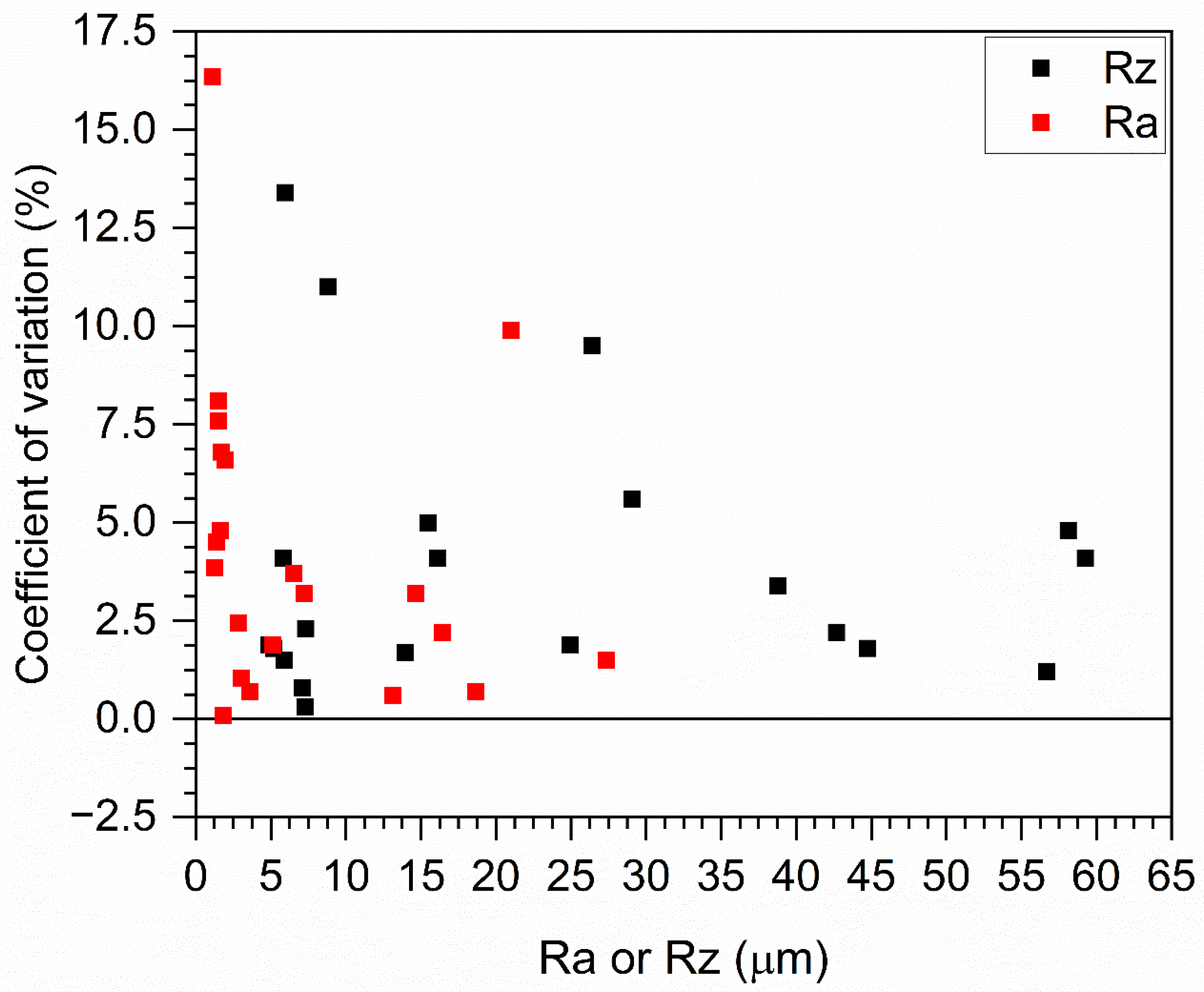
3. Results and Discussion

3.1. Roughness Measurements

Table 1. Average user-measured Ra and Rz values with associated standard deviation, as well as a comparison between standard deviation and average value. Deviations over 5% marked in bold.

	User-Measured Values
	Rz (μm)			Ra (μm)
Image	Average	Standard Deviation (s)	100 × CV	Average	Standard Deviation (s)	100 × CV
1	26.42	2.5095	9.5	5.102	0.0974	1.9
2	29.04	1.6308	5.6	7.201	0.2306	3.2
3	24.95	0.4812	1.9	6.536	0.2429	3.7
4	44.73	0.807	1.8	13.106	0.0773	0.6
5	42.68	0.951	2.2	18.63	0.135	0.7
6	38.78	1.311	3.4	14.63	0.465	3.2
7	7.29	0.023	0.3	1.95	0.129	6.6
8	7.11	0.055	0.8	1.61	0.078	4.8
9	5.89	0.090	1.5	1.48	0.121	8.1
10	56.67	0.703	1.2	16.44	0.359	2.2
11	59.26	2.458	4.1	27.37	0.413	1.5
12	58.11	2.812	4.8	21.00	2.084	9.9
13	4.87	0.095	1.9	1.40	0.064	4.5
14	5.20	0.096	1.8	1.81	0.003	0.1
15	5.97	0.803	13.4	1.67	0.114	6.8
16	7.32	0.168	2.3	1.24	0.048	3.85
17	5.81	0.237	4.1	1.10	0.179	16.35
18	8.82	0.970	11.0	1.52	0.116	7.6
19	15.49	0.777	5.0	3.05	0.032	1.05
20	16.08	0.659	4.1	3.50	0.026	0.7
21	13.97	0.240	1.7	2.81	0.068	2.45

shows the average Rz and Ra values measured by the users for each image and the associated standard deviation. Each column, therefore, represents the average roughness measured by the three users for a single image. The coefficient of variation (CV) is lower than 5% for Ra and Rz in most cases, independently of the roughness. For Rz, the coefficient is over 5% in only 4 of the 21 images, and for Ra, in 6 of the 21 images. For Rz, the first two images are examples of larger errors caused by differences in how each user applied the method, as will be discussed later. Notable exceptions for Ra are image 12, due to differences in how the users interpreted the metal/oxide interface, and image 17, which had the lowest Ra value and was, therefore, harder for the users to analyze (higher resolution images would be needed). A visualization of the CV as a function of Ra or Rz can be seen in Figure 5. It is clear that the higher coefficients of variation tend to be associated with samples with lower Ra or Rz.

Table 2. Ra and Rz values measured by the algorithm, as well as a 99% confidence interval corresponding to user measurements. Algorithm values outside the confidence interval are in bold.

	Algorithm		99% Confidence Interval (User Measurements) (Min; Max)
Image	Rz (μm)	Ra (μm)	Rz (μm)	Ra (μm)
1	20.93	4.81	(12.04; 40.79)	(4.54; 5.66)
2	24.11	5.84	(19.70; 38.39)	(5.88; 8.52)
3	22.32	6.39	(22.19; 27.70)	(5.15; 7.93)
4	41.06	11.99	(40.10; 49.35)	(12.66; 13.55)
5	44.30	18.45	(37.23; 48.13)	(17.86; 19.41)
6	36.62	14.00	(31.27; 46.29)	(11.97; 17.29)
7	6.49	1.55	(7.15; 7.42)	(1.21; 2.69)
8	6.29	1.32	(6.80; 7.43)	(1.17; 2.06)
9	5.70	1.07	(5.38; 6.41)	(0.79; 2.18)
10	49.27	15.99	(52.65; 60.70)	(14.38; 18.50)
11	50.46	27.31	(45.17; 73.34)	(25.00; 29.73)
12	45.56	17.58	(41.99; 74.22)	(9.06; 32.94)
13	4.37	1.24	(3.94; 5.64)	(1.03; 1.76)
14	5.10	1.61	(3.11; 6.92)	(1.80; 1.83)
15	5.63	1.35	(2.32; 9.35)	(1.02; 2.32)
16	6.42	1.02	(6.35; 8.28)	(0.96; 1.51)
17	5.23	0.81	(4.45; 7.17)	(0.07; 2.12)
18	7.68	1.33	(3.27; 14.38)	(0.86; 2.19)
19	14.24	2.73	(11.04; 19.95)	(2.86; 3.23)
20	12.19	3.27	(12.30; 19.86)	(3.44; 3.74)
21	12.19	2.53	(12.60; 15.35)	(2.42; 3.20)

shows the algorithm-measured values and the confidence interval for the user-measured Ra and Rz values for comparison. The values that are outside their respective confidence interval are marked in bold; 5 of the 21 values for Rz and Ra are marked (23.8%). Only in image 20 are Rz and Ra simultaneously marked. The significant difference between user and algorithm values is related to the fact that the algorithm tends to smooth large peaks and valleys, as will be discussed later. Note, however, that a similar effect would be present if conventional contact measurement techniques were used, as these techniques are limited by the radius of the probe tip and the need for the probe to be able to make contact with the surface. This is a characteristic that was shown to cause significant differences between contact and image analysis techniques for roughness measurement [25].

Figure 6 summarizes the previously discussed Rz (a) and Ra (b) values, comparing the user measurements, with their associated confidence intervals, to the algorithm-derived values. Notably, all algorithm values that fell outside the confidence intervals were on the lower end, and even those within the interval tended to lie close to the lower bound or at least below the user-measured average. This trend indicates that the algorithm generally produces lower roughness values compared with manual measurements.

Another observation from Figure 6 is the considerable width of the confidence intervals in several cases (Images 11 and 12, for example). This can be attributed to the limited number of users (three), the variability in manual measurements, and the use of a conservative 99% confidence level. Overall, the relatively large dispersion in user measurements reinforces that while manual methods can capture fine interfacial details, they are also subject to a high degree of user interpretation and variability.

Despite the systematic underestimation, values measured by the algorithm closely follow the trend observed in the manual measurements. At no point did the discrepancies due to algorithm smoothing or variability among users compromise the comparative interpretation of roughness across samples. For example, both methods clearly indicate that sample 4 (images 10–12) is rougher than sample 1 (images 1–3). As previously established, each group of three images corresponds to a single experimental condition. Thus, in

Table 3. Average Ra and Rz measurements for each of the seven samples. The value taken for the users is the average of all user measurements. Samples are ranked from highest to lowest roughness. Cases in which the ranking order is different for the User and Algorithm measurements are marked in bold.

	Rz (μm)				Ra (μm)
	User		Algorithm		User		Algorithm
Sample	Average	Ranking	Average	Ranking	Average	Ranking	Average	Ranking
1 (1–3)	26.80	3	22.45	3	6.28	3	5.68	3
2 (4–6)	42.06	2	40.66	2	15.46	2	14.81	2
3 (7–9)	6.76	6	6.16	6	1.68	5	1.31	6
4 (10–12)	58.01	1	48.43	1	21.60	1	20.29	1
5 (13–15)	5.34	7	5.03	7	1.63	6	1.40	5
6 (16–18)	7.32	5	6.44	5	1.29	7	1.05	7
7 (19–21)	15.18	4	12.87	4	3.15	4	2.84	4

, the final average roughness values for each sample are ranked from highest to lowest according to both the users (manually) and the algorithm. Although the absolute values differ, the rankings are consistent. The sole exceptions are samples 3 (images 7 to 9) and 5 (13 to 15), which are swapped in the Ra rankings between the two methods. However, the difference in Ra between samples is minimal (0.05 μm according to the users and 0.09 μm by the algorithm), which is close to the resolution limit of the images used in this study. This discrepancy is therefore negligible and does not indicate a relevant disagreement between the two methods.

3.2. Influence of Threshold Value on Algorithm Measurements

The percentual difference between the value measured with a threshold of 20 and values measured with thresholds representing 10, 25, and 50% variation in both directions (18 and 22, 15 and 25, and 10 and 30, respectively) are shown in Figure 7 for Rz (a) and Ra (b). A threshold of 20 was chosen as the standard value because, for the images studied here, it always gave acceptable results. It appears that the variation only reaches significant values with extreme skewing of the threshold (10 and 30). For non-extreme values, the variation is usually below 10%, indicating that the algorithm is mostly robust to the threshold choice. The exceptions are the Rz measurement of image 15 for a threshold of 15 and the Rz measurement for a threshold of 15 of image 21. The errors are related to the smooth surface of the first and the significant variation in gray value on the substrate of the second. Both phenomena will be discussed in detail.

In conclusion, a single threshold value (20) was successfully applied across all images, demonstrating the consistency of the method. Small deviations (e.g., 18 or 22) generally had a negligible impact on the roughness measurements, and when they did introduce significant changes, such as in sample 21, the error was clear to the user during the selection process, as the selected “interface” clearly did not correspond to the actual interface. These findings confirm that the algorithm effectively reduces user-induced variability to near zero by standardizing the interface selection process. For this reason, results obtained by different users applying the algorithm were not presented or discussed, as following the standard procedure necessarily led to negligible differences in measured values.

3.3. Main Sources of Variance in Measurements

As previously said, smoother interfaces led to higher coefficients of variation in the user-measured values. This is especially true for the Ra values and mainly a consequence of the fact that, in this study, all images were taken at the same magnification. As seen in Figure 8, the magnification is sufficient to analyze rough interfaces (b), but a lot of detail is lost on smoother ones (a). A possible option for eliminating this problem is to take separate images and then combine them, effectively increasing the pixel count at the interface. For the images used in this study, the pixels had sides of 0.33 μm. For the images with an Rz of 6 μm or below, for example, this means that less than 20 pixels, on average, separated the peaks from the valleys. Consequently, any difference between the pixels selected by the users can translate to a more significant difference in results (5%, at least). On the other hand, for the higher values of Rz ranging from 40 to 60 μm, 1 pixel represents less than 1% of the peak-to-valley distance. The use of the algorithm mitigated the difficulty the users had in discerning details of the interface by limiting their input to selecting the threshold. In general, changing the threshold did not have a particularly significant effect on samples with low roughness compared with those with rougher interfaces. However, the precision of the measurements, in practice, was still reduced by the low resolution of the images. Thus, it is recommended that higher magnifications be used for smoother samples.

3.3.1. Gray Value Differences in the Interface and in the Selected Region

Gray value differences between parts of the image affected the algorithm in significant ways, but adequate user input mitigated this effect. The most common type of variation was caused by defects or grain boundaries that appear as regions with clearly different gray values. When these anomalous regions were present at the edge of the image, the selection tool was unable to select them, as Figure 9 shows. In Figure 9a, it is possible to see the Scanning Electron Microscopy (SEM) image with a shadow on the lower left side. After masking, in Figure 9b, the shadow is not completely selected by the threshold tool, leaving a black area inside the substrate. Considering that the algorithm works by stacking gray values, this area would significantly deform the roughness profile. To solve this problem, users can select these regions, and the algorithm will fill them with the gray value of the point they selected in the first step. As seen in Figure 9c, applying the correction leads to adequate masking.

The second type of gray value variation occurred in samples where the substrate itself exhibited significant internal variation (due to different phases or grain orientations, for example) or where there was low contrast between the substrate and the oxide. In these cases, the sensitivity of the thresholding step increased. If the internal gray value differences within the substrate are too large, a single threshold may fail to capture the entire region, depending on where the user initially clicks. Figure 10 illustrates an extreme case, where the metal/oxide interface is clearly visible (Figure 10a) and is first correctly selected with a threshold of 20 (Figure 10b). However, when heavily skewed thresholds are used (5 and 35), the selection fails (Figure 10c,d) to fully outline the interface.

In most of the images analyzed in this study, the average gray value variation within the substrate was considerably low. Thus, a ±2 variation in threshold around the standard value (20) had little impact on the results (as seen in Figure 7). However, in cases with more pronounced internal variation, even small changes in threshold or a poorly chosen starting point can lead to inadequate selections. This underscores the importance of human input, as the approach presented here requires that the user visually confirm that the selected threshold accurately outlines the interface. If not, they can adjust the threshold or select a different initial point that better represents the average gray level of the substrate.

3.3.2. Peaks and Valleys with Complex Shapes

The largest differences between user-measured roughness were observed in discontinuous or almost discontinuous interfaces. In these cases, some users opted to consider parts of the metal that, in the image, appear isolated in the oxide layer as part of the interface. The same is valid for parts of the oxide layer isolated in the metallic substrate. The effect of this on Ra measurements can be seen in Figure 11. The figure shows the mean line height defined by User 1. With this line, User 1 calculated the area of oxide below the line to be 4012 μm² and the area of metal above the interface to be 5349 μm². User 2 defined the line at almost the same position, indicating that, while selecting the substrate area to define the mean line height, both users had the same approach. This should translate to a similar measurement, and, in fact, the user measured the oxide area below the line to be 3971 μm², almost the same value as User 1. However, the area of metal above the line was 3950 μm², a very significant difference. The reason for this difference can be seen in the circle A marked in red in Figure 11. This metallic area is almost completely separated from the substrate, and neither user considered it to be part of the interface while defining the mean line. User 1, however, later added this area to the total area above the line, significantly changing the measured value.

The same image also presented issues for the Rz measurement, as seen in Figure 12. Although rectangles 2 to 5 have similar heights, the first user considered the isolated metallic region to be part of the substrate, which caused rectangle 1 to be much higher and the overall Rz to increase.

In the image presented in Figure 13, the larger standard deviation is caused by a similar problem. However, in this case, the divergence between the users stemmed from a region of oxide isolated inside the substrate (indicated in 1). For User 1, the region was considered part of the interface, while for User 2, it was not. This caused a large variation in the measured height of Rectangle 5. Notably, the average Rz values are close despite this discrepancy. This is caused by another difference in interpretation, related to Rectangle 1, to which User 2 attributed a larger height than User 1. In this rectangle, there is a thin protrusion of metal entering the oxide layer. It is difficult to define if this protrusion is connected to the substrate and, if so, where exactly it ends. It is a similar source of variability to the one discussed in Figure 12. Despite the aforementioned sources of variability, disagreements between the location of the interface do not usually lead to such large discrepancies, as can be observed in rectangles 2 to 4. The chosen endpoint of the highest peak is slightly different between the users, but the height values are still close.

Naturally, isolated regions of metal or oxide cannot be selected by the algorithm, as it relies on continuous contrast in grayscale values to define the interface. This limitation is consistent with the manual measurement guidelines discussed previously, which instruct users to ignore isolated portions. In the case of the algorithm, the primary reason for the different values between manual and automated measurements is its inability to interpret complex-shaped peaks and valleys, particularly those with curved or geometric shapes. This limitation becomes evident when comparing the ImageJ-generated profile to the original microscope image, as shown in Figure 14. The “Plot Profile” function in ImageJ constructs a roughness profile by averaging gray values, effectively “stacking” pixel intensity columns to define the vertical (Y-axis) profile. As a result, curved or sloped features are smoothed. For instance, if a peak curves outward (as indicated in region 1 of Figure 14), the algorithm will miss this detail, underestimating both Rz (peak-to-valley height) and altering the position of the mean line used for calculating Ra (average roughness).

This smoothing is an inherent limitation of the ImageJ method and cannot be fully corrected without major changes or even the use of more powerful image analysis algorithms. Importantly, similar simplifications also occur in conventional contact-based profilometry: stylus tips, due to their geometry, cannot detect recessed or overhanging features and instead trace only the outermost contours [32]. Therefore, while this limitation affects the accuracy of complex peak measurements, it is not unique to the digital method.

3.4. Error Propagation and Traceability in the Measurement Workflow

To conclude the discussion of the measurement process, it is useful to provide a comprehensive overview of the entire workflow, from sample preparation to final roughness values, highlighting the potential for information loss during each stage and how such loss can be tracked or minimized. A flowchart summarizing this workflow and the sources of information loss is presented in Figure 15. The process begins with sample preparation, typically involving cross-sectioning, mounting, and polishing, followed by image acquisition. While polishing is a potential source of information loss (e.g., interface smearing or deformation), this is easily avoidable through proper metallographic procedures. By contrast, image acquisition represents an inherent and non-negligible source of information loss. During this stage, the three-dimensional physical interface is reduced to a two-dimensional digital grayscale image. The fidelity of this representation depends on multiple factors, such as image resolution, magnification, and the achievable resolution of the technique used to acquire the image. Because the precision of all subsequent measurements is fundamentally constrained by the digital representation of the interface, image acquisition must be approached with particular care.

Once acquired, images are scaled and cropped, defining the physical dimensions (e.g., µm per pixel) and the region of interest. If representative images are selected and the scaling is applied correctly, this step does not introduce additional error. Next comes thresholding, the most critical and user-dependent phase of the process. Here, the user selects the region corresponding to the substrate based on contrast and is also able to manually correct edge defects. Because the accuracy of this step directly determines how faithfully the interface is outlined, it is important that the user is able to visually assess and iteratively refine the selection before proceeding, granting full control over this potentially error-prone stage. Following thresholding, the masking and calculation steps are executed automatically (the user is only responsible for exporting the generated profile and running the calculation script). In masking, gray values are binarized, simplifying the image into two distinct levels. The generation of a profile based on average gray value from this masked image introduces some unavoidable information loss, as previously discussed. The subsequent calculation step, based on the implementation of traditional equations for the desired roughness parameters, does not represent a significant source of loss. Crucially, the user maintains control over all major sources of measurement uncertainty: sample preparation, image acquisition, and thresholding. The only step in which information loss cannot be entirely avoided is during masking.

4. Conclusions

Given adequate image resolution, both techniques developed in this study were capable of determining the position and approximate shape of the interface between two layers, allowing for standardized roughness measurements. The manual method is intuitive and accessible, making it suitable for didactic and exploratory purposes. However, its high susceptibility to user interpretation introduced considerable variability into the results. This limitation was mitigated in the semi-automated method, which integrates an ImageJ macro with an R-language script. While still requiring minimal user input (color threshold selection for substrate identification), the subsequent steps are fully automated. This hybrid approach strikes an effective balance, retaining the interpretative capacity necessary for analyzing complex interfaces while significantly reducing variability. Although the algorithm tends to underestimate absolute roughness values by smoothing sharp features and curved peaks, this behavior is consistent with limitations of traditional contact-based profilometry. Importantly, the method preserved the relative ranking of roughness across all samples when compared with user measurements, which is often more relevant in comparative studies. The open-source and modular nature of the method also enhances its versatility, as it can be adapted to different image sources, analysis workflows, or specific applications (e.g., coatings, oxide layers). Its capability to analyze interfaces that are otherwise inaccessible to contact methods is a significant practical advantage. Also, as indicated by the significant differences in selected areas when the substrate had variations in color, maintaining user input is a valuable improvement over fully automated methods.

In future studies, the current method could serve as a foundation for the development of machine learning tools trained specifically to recognize and evaluate a particular type of interface. By incorporating user input, the method presented here naturally generates labeled datasets that reflect human interpretations of complex or ambiguous features. These datasets could then be used to train supervised models that replicate human-guided interface identification in similar materials or imaging conditions. Such an approach would preserve the interpretive nuance of the current method while increasing throughput for large-scale studies. Importantly, the goal should not be to fully replace user interaction but to extend the current framework by allowing faster processing of new images once an appropriate interface model has been trained.

References

1. Whitesides, D.J. Handbook of Surface and Nanometrology; CRC Press: Boca Raton, FL, USA, 2011. [Google Scholar]
2. Galedari, S.A.; Mahdavi, A.; Azarmi, F.; Huang, Y.; McDonald, A. A Comprehensive Review of Corrosion Resistance of Thermally-Sprayed and Thermally-Diffused Protective Coatings on Steel Structures. J. Therm. Spray Technol. 2019, 28, 645–677. [Google Scholar] [CrossRef]
3. Nazeer, A.A.; Madkour, M. Potential Use of Smart Coatings for Corrosion Protection of Metals and Alloys: A Review. J. Mol. Liq. 2018, 253, 11–22. [Google Scholar] [CrossRef]
4. Mah, J.C.W.; Muchtar, A.; Somalu, M.R.; Ghazali, M.J. Metallic Interconnects for Solid Oxide Fuel Cell: A Review on Protective Coating and Deposition Techniques. Int. J. Hydrogen Energy 2017, 42, 9219–9229. [Google Scholar] [CrossRef]
5. Rizwan, M.; Alias, R.; Zaidi, U.Z.; Mahmoodian, R.; Hamdi, M. Surface Modification of Valve Metals Using Plasma Electrolytic Oxidation for Antibacterial Applications: A Review. J. Biomed. Mater. Res. Part A 2018, 106, 590–605. [Google Scholar] [CrossRef] [PubMed]
6. Nicholls, J.R.; Bennett, M.J. Cyclic Oxidation—Guidelines for Test Standardisation, Aimed at the Assessment of Service Behaviour†. Mater. High Temp. 2000, 17, 413–428. [Google Scholar] [CrossRef]
7. Silva, R.; Vacchi, G.S.; Santos, I.G.R.; Malafaia, A.d.S.; Kugelmeier, C.L.; Filho, A.A.M.; Pascal, C.; Sordi, V.L.; Rovere, C.A.D. Insights into High-Temperature Oxidation of Fe-Mn-Si-Cr-Ni Shape Memory Stainless Steels and Its Relationship to Alloy Chemical Composition. Corros. Sci. 2020, 163, 108269. [Google Scholar] [CrossRef]
8. Zhang, X.; Mo, J.; Si, Y.; Guo, Z. How Does Substrate Roughness Affect the Service Life of a Superhydrophobic Coating? Appl. Surf. Sci. 2018, 441, 491–499. [Google Scholar] [CrossRef]
9. Hagen, C.M.H.; Hognestad, A.; Knudsen, O.Ø.; Sørby, K. The Effect of Surface Roughness on Corrosion Resistance of Machined and Epoxy Coated Steel. Prog. Org. Coat. 2019, 130, 17–23. [Google Scholar] [CrossRef]
10. Croll, S.G. Surface Roughness Profile and Its Effect on Coating Adhesion and Corrosion Protection: A Review. Prog. Org. Coat. 2020, 148, 105847. [Google Scholar] [CrossRef]
11. Ostwald, C.; Grabke, H.J. Initial Oxidation and Chromium Diffusion. I. Effects of Surface Working on 9–20% Cr Steels. Corros. Sci. 2004, 46, 1113–1127. [Google Scholar] [CrossRef]
12. Guttmann, V.; Hukelmann, F.; Griffin, D.; Daadbin, A.; Datta, S. Studies of the Influence of Surface Pre-Treatment on the Integrity of Alumina Scales on MA 956. Surf. Coat. Technol. 2003, 166, 72–83. [Google Scholar] [CrossRef]
13. Sudbrack, C.K.; Beckett, D.L.; Mackay, R.A. Effect of Surface Preparation on the 815 °C Oxidation of Single-Crystal Nickel-Based Superalloys. J. Miner. Met. Mater. Soc. 2015, 67, 2589–2598. [Google Scholar] [CrossRef]
14. Platt, P.; Allen, V.; Fenwick, M.; Gass, M.; Preuss, M. Observation of the Effect of Surface Roughness on the Oxidation of Zircaloy-4. Corros. Sci. 2015, 98, 1–5. [Google Scholar] [CrossRef]
15. Malafaia, A.M.d.S.; Nascimento, V.R.D.; Sousa, L.M.; Silveira, M.E.; de Oliveira, M.F. Anomalous Cyclic Oxidation Behaviour of an Fe-Mn-Si-Cr-Ni Alloy—A Finite Element Analysis. Corros. Sci. 2019, 147, 223–230. [Google Scholar] [CrossRef]
16. Malafaia, A.M.d.S.; de Oliveira, M.F. Anomalous Cyclic Oxidation Behaviour of a Fe–Mn–Si–Cr–Ni Shape Memory Alloy. Corros. Sci. 2017, 119, 112–117. [Google Scholar] [CrossRef]
17. Rabelo, L.; Silva, R.; Della Rovere, C.; Malafaia, A.d.S. Metal/Oxide Interface Roughness Evolution Mechanism of an FeMnSiCrNiCe Shape Memory Stainless Steel under High Temperature Oxidation. Corros. Sci. 2020, 163, 108228. [Google Scholar] [CrossRef]
18. Pindera, M.-J.; Aboudi, J.; Arnold, S.M. The Effect of Interface Roughness and Oxide Film Thickness on the Inelastic Response of Thermal Barrier Coatings to Thermal Cycling. Mater. Sci. Eng. A 2000, 284, 158–175. [Google Scholar] [CrossRef]
19. Ahrens, M.; Vaßen, R.; Stöver, D. Stress Distributions in Plasma-Sprayed Thermal Barrier Coatings as a Function of Interface Roughness and Oxide Scale Thickness. Surf. Coat. Technol. 2002, 161, 26–35. [Google Scholar] [CrossRef]
20. Li, Y.; Gao, H.; Wang, L.; Sun, Y.; Zhang, J. Discrete Element Modeling of Effect of Interfacial Roughness and Pre-Crack on Crack Propagation in Thermal Barrier Coatings. Comp. Part. Mech. 2025, 12, 31–39. [Google Scholar] [CrossRef]
21. Ferguen, N.; Leclerc, W.; Lamini, E.-S. Numerical Investigation of Thermal Stresses Induced Interface Delamination in Plasma-Sprayed Thermal Barrier Coatings. Surf. Coat. Technol. 2023, 461, 129449. [Google Scholar] [CrossRef]
22. Carim, A.H.; Sinclair, R. The Evolution of Si/SiO2 Interface Roughness. J. Electrochem. Soc. 1987, 134, 741–746. [Google Scholar] [CrossRef]
23. Bossis, P.; Lefebvre, F.; Barbéris, P.; Galerie, A. Corrosion of Zirconium Alloys: Link between the Metal/Oxide Interface Roughness, the Degradation of the Protective Oxide Layer and the Corrosion Kinetics. Mater. Sci. Forum 2001, 369–372, 255–262. [Google Scholar] [CrossRef]
24. Platt, P.; Wedge, S.; Frankel, P.; Gass, M.; Howells, R.; Preuss, M. A Study into the Impact of Interface Roughness Development on Mechanical Degradation of Oxides Formed on Zirconium Alloys. J. Nucl. Mater. 2015, 459, 166–174. [Google Scholar] [CrossRef]
25. Roux, S.L.; Deschaux-Beaume, F.; Cutard, T.; Lours, P. Quantitative Assessment of the Interfacial Roughness in Multi-Layered Materials Using Image Analysis: Application to Oxidation in Ceramic-Based Materials. J. Eur. Ceram. Soc. 2015, 35, 1063–1079. [Google Scholar] [CrossRef]
26. Ridley, M.; Garcia, E.; Kane, K.; Sampath, S.; Pint, B. Environmental Barrier Coatings on Enhanced Roughness SiC: Effect of Plasma Spraying Conditions on Properties and Performance. J. Eur. Ceram. Soc. 2023, 43, 6473–6481. [Google Scholar] [CrossRef]
27. Chikhalikar, A.S.; Godbole, E.P.; Poerschke, D.L. Approach for Statistical Analysis of Oxide- and Sulfate-Induced Hot Corrosion of Advanced Alloys. Corros. Sci. 2023, 211, 110892. [Google Scholar] [CrossRef]
28. Paksoy, A.H.; Scotson, D.; Yilmaz, E.; Xiao, P. Interfacial Characteristics and Adhesion Behaviour of Ytterbium Silicate Environmental Barrier Coatings Exposed to Steam Oxidation. Corros. Sci. 2025, 251, 112879. [Google Scholar] [CrossRef]
29. Stegmueller, M.J.R.; Grant, R.J.; Schindele, P. Quantification of the Interfacial Roughness When Coating Stainless Steel onto Aluminium by Friction Surfacing. Surf. Coat. Technol. 2019, 375, 22–33. [Google Scholar] [CrossRef]
30. Balachandran, S.; Smathers, D.B.; Kim, J.; Sim, K.; Lee, P.J. A Method for Measuring Interface Roughness from Cross-Sectional Micrographs. IEEE Trans. Appl. Supercond. 2023, 33, 1–5. [Google Scholar] [CrossRef]
31. Gadelmawla, E.S.; Koura, M.M.; Maksoud, T.M.A.; Elewa, I.M.; Soliman, H.H. Roughness Parameters. J. Mater. Process. Technol. 2002, 123, 133–145. [Google Scholar] [CrossRef]
32. O’Donnell, K.A. Effects of Finite Stylus Width in Surface Contact Profilometry. Appl. Opt. 1993, 32, 4922. [Google Scholar] [CrossRef] [PubMed]
Figure 1. Ra and Rz measurement method. In (a), the selection of rectangles for Rz measurement, and in (bd), the selection of areas of metal above the mean line and oxide below.
Cmd 06 00031 g001
Figure 2. Operation of the tool for scaling and cropping the image to a standardized size.
Cmd 06 00031 g002
Figure 3. Step-by-step view of the roughness profile generation. First, the cropped image is opened (a); then the user selects the threshold, seen as the yellow outline (b); the image is then cropped to a standard height and masked (c); and the profile is generated (d).
Cmd 06 00031 g003
Figure 4. Transformation of the masked image into a roughness profile and mathematical operations used to calculate Ra and Rz from it. In (a), the masked image contains two regions, divided by the interface of interest and with two distinct grayscale values. In (b), the gray values are averaged, effectively giving rise to a roughness profile. In (c), the profile is used to calculate ta, and in (d), to calculate Rz.
Cmd 06 00031 g004
Figure 5. Coefficient of variation of the average Ra and Rz measurements taken manually by three users in this study.
Cmd 06 00031 g005
Figure 6. User-measured values (with the confidence interval, or CI) compared with algorithm-measured values for Rz (a) and Ra (b). The algorithm values (represented by X) were colored according to their alignment with the user-measured values. Thus, images in which the algorithm measurement was inside the CI for Ra or Rz were colored in blue. If both Ra and Rz for a given image were inside the CI, green was used.
Cmd 06 00031 g006
Figure 7. Variation between Rz (a) and Ra (b) values measured with the standard threshold (20) and thresholds 10, 25, and 50% higher or lower.
Cmd 06 00031 g007
Figure 8. Comparison between a smooth (a) and a rough interface (b) analyzed in this study.
Cmd 06 00031 g008
Figure 9. Substrate with an edge artifact of different coloration (a) and artifact not being correctly selected (b). Using the correction tool, the substrate is adequately represented (c).
Cmd 06 00031 g009
Figure 10. Algorithm applied to an example substrate (a) with the correct threshold selection (b), insufficient selection (c), and excessive selection (d).
Cmd 06 00031 g010
Figure 11. Interface with a region of oxide separated from the substrate (A), which was not considered by one user when calculating the area of metal above the white line but was considered by another, leading to different Ra measurements.
Cmd 06 00031 g011
Figure 12. Rz measurements for the shown substrate, indicating significant variation in rectangles 1 and 3 due to different interpretations concerning the location of the metal/oxide interface, due to a region of metal isolated from the substrate. Each rectangle in the figure represents a measurement length of 80 μm.
Cmd 06 00031 g012
Figure 13. Rz measurements for the shown substrate, indicating significant variation in rectangles 1 and 5 due to different interpretations concerning the location of the metal/oxide interface due to a region of oxide isolated from the substrate (1). Notice how the error is masked on the final Rz value, as it is an average of all five values. Each rectangle in the figure represents a measurement length of 80 μm.
Cmd 06 00031 g013
Figure 14. Comparison between the real metal/oxide interface and the interface as seen by the algorithm. Complex-shaped regions, such as those in 1, are smoothed by the algorithm.
Cmd 06 00031 g014
Figure 15. Flowchart detailing the roughness measurement process, from sample preparation to the calculation of the roughness parameters from the extracted profile. The flowchart also details the processes done at each step and the sources of information loss.
Cmd 06 00031 g015