
Validation of Water Radiolysis Models Against Experimental Data in Support of the Prediction of the Radiation-Induced Corrosion of Copper-Coated Used Fuel Containers


Abstract
1. Introduction
2. Background
2.1. Overview of CCM-RIC
2.2. Treatment of Mass Transfer at the Gas–Solution Interface
2.3. Comparison of Different Chloride Radiolysis Models
3. Software and Description of Validation Simulations
3.1. Software
3.2. Validation Simulations
4. Results and Discussions of Validation Simulations
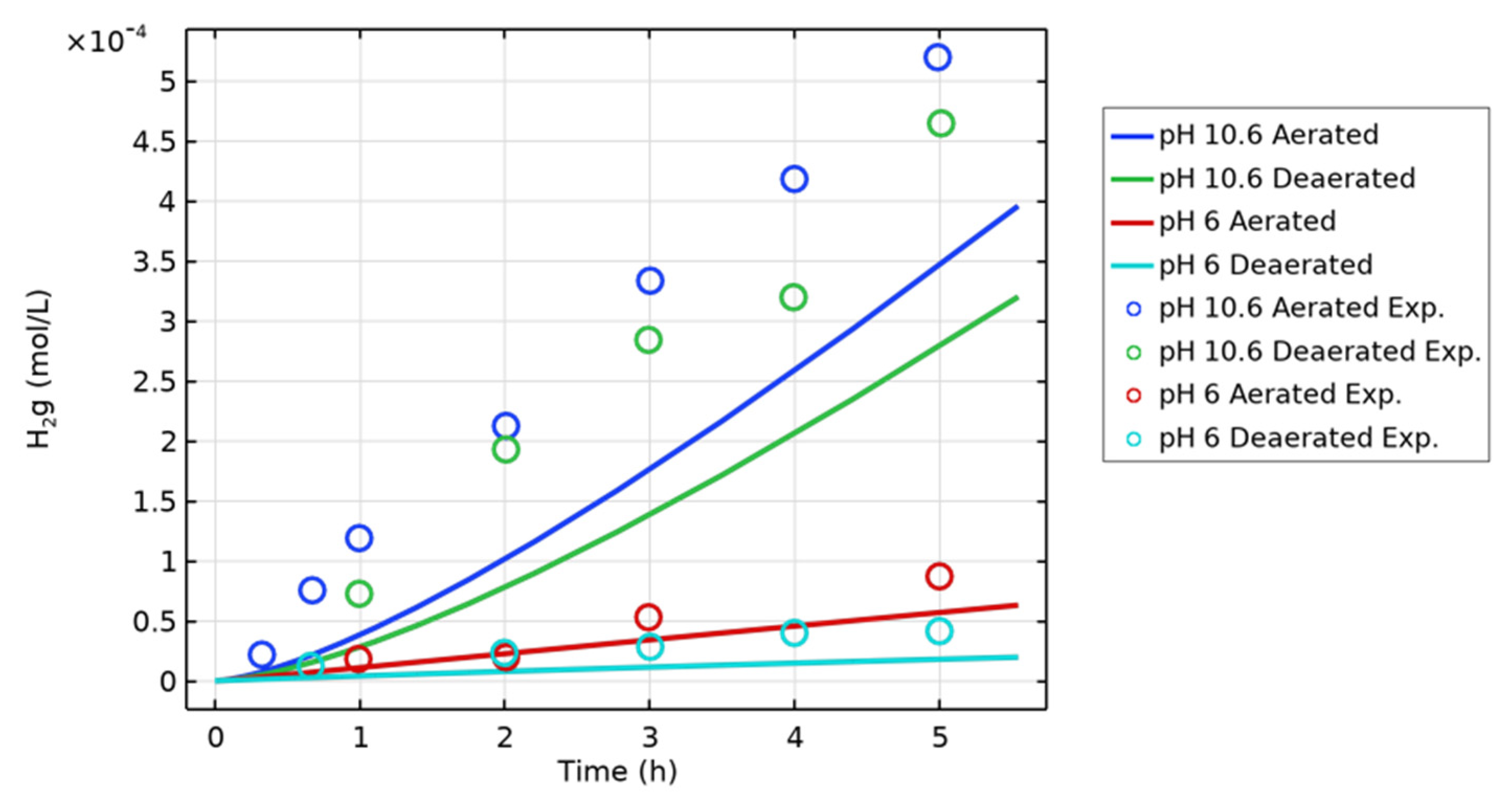
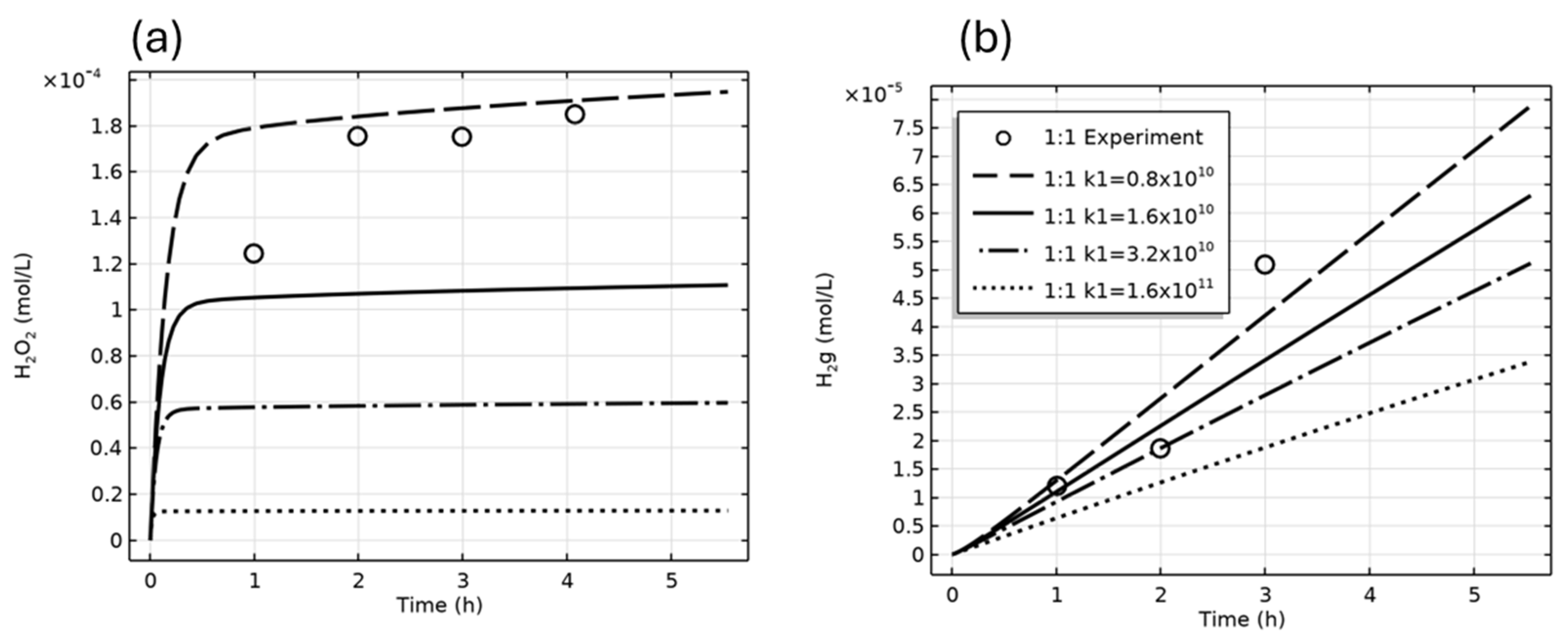
4.1. Pure H2O, Mass Transfer at the Gas–Solution Interface
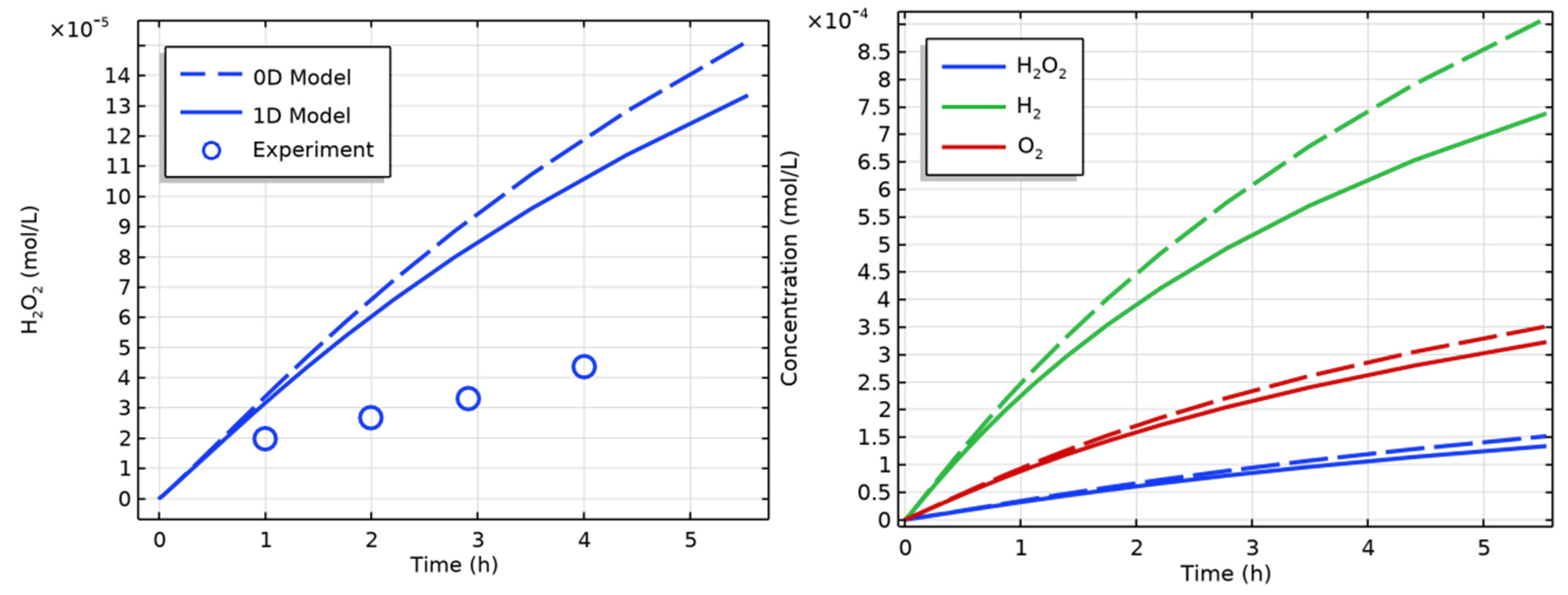
4.2. Comparison of Models with and Without a Headspace
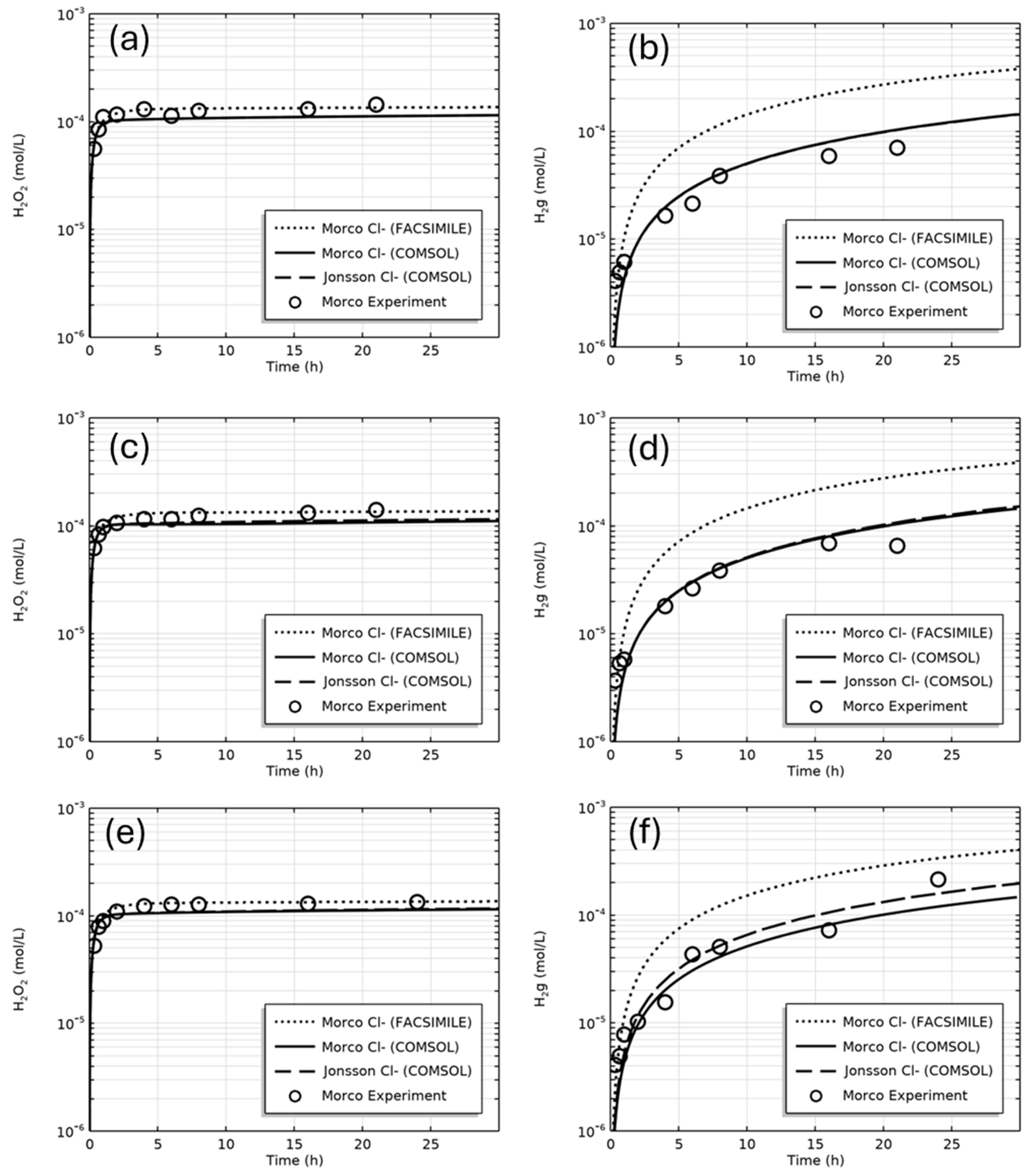
4.3. Comparison of Chloride Radiolysis Models
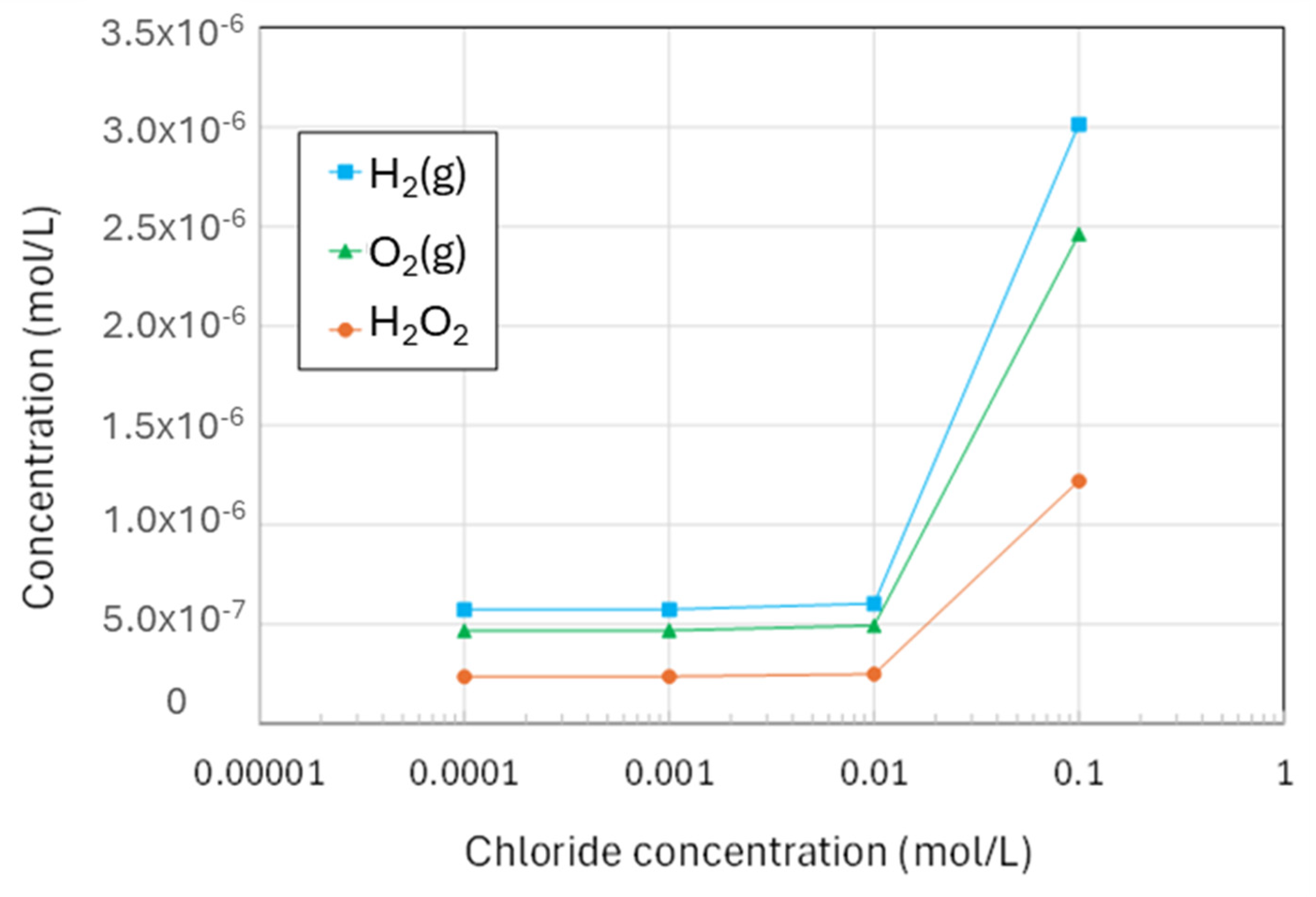
4.4. Effect of Chloride on the Production of Molecular Radiolysis Products
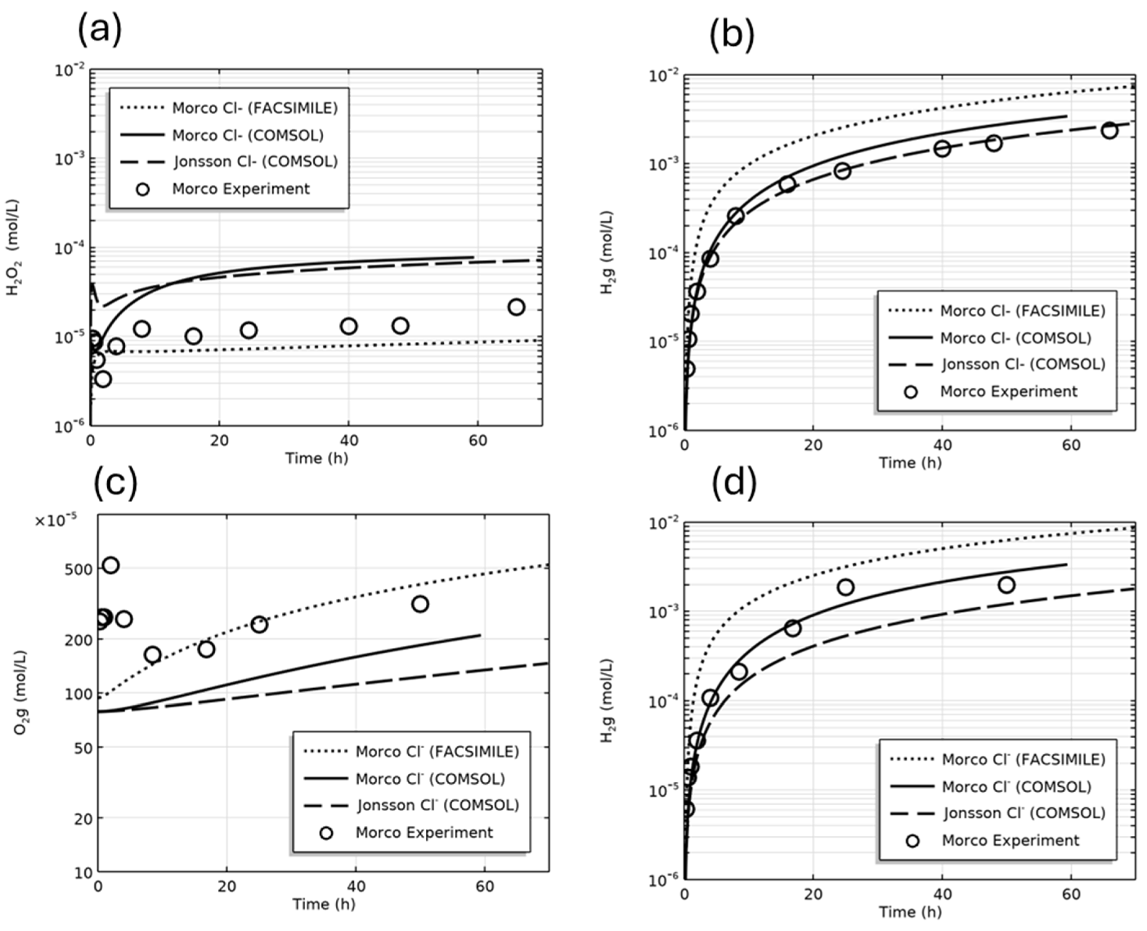
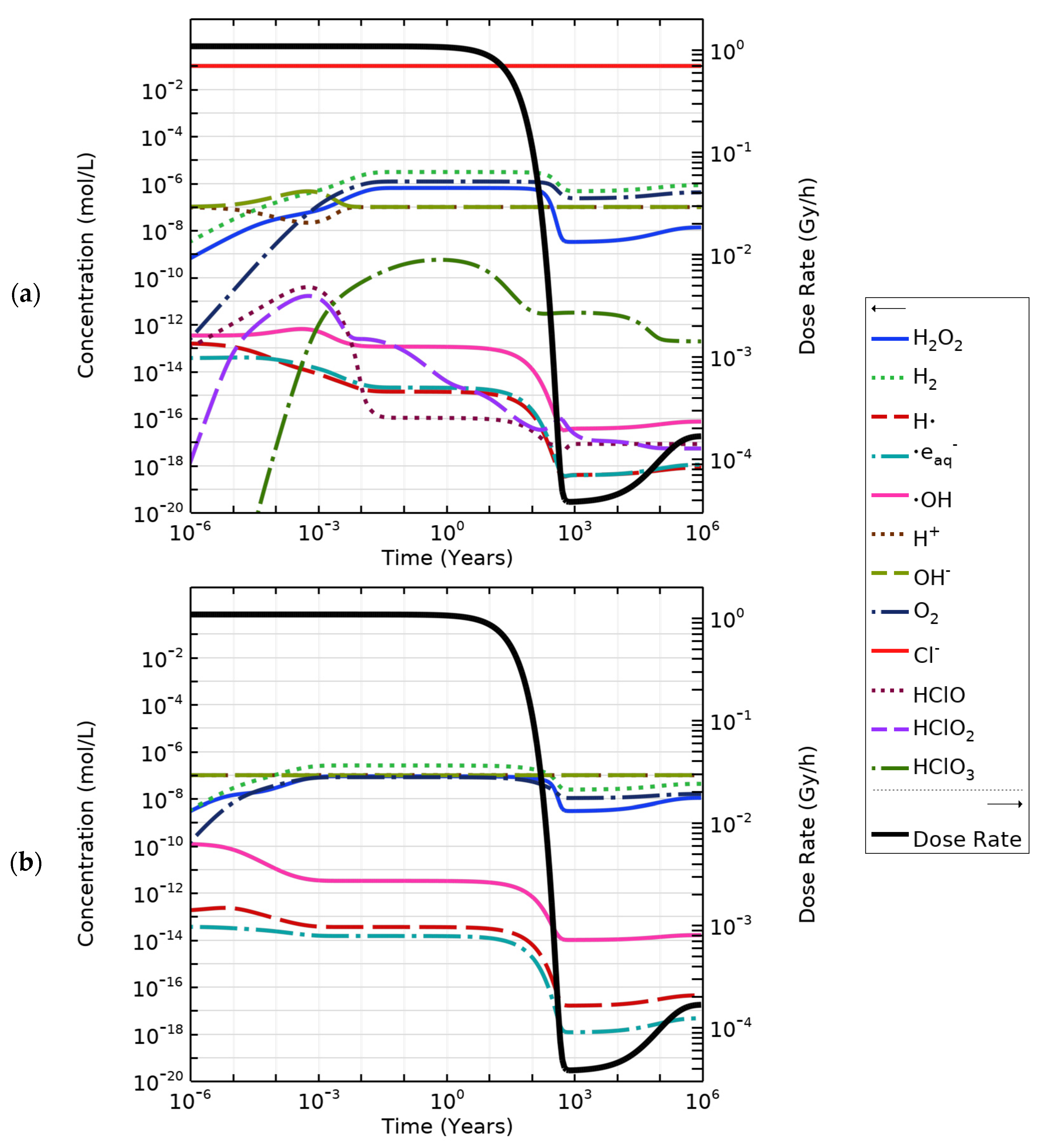
4.5. Concentrations of Radiolysis Products Under Repository Conditions
5. Conclusions
Author Contributions
Funding
Data Availability Statement
Acknowledgments
Conflicts of Interest
Appendix A

| Reactants | Products | k (dm3 mol−1 s−1) or (s−1) |
|---|---|---|
| •OH + Cl− | •ClOH− | 4.3 × 10⁹ |
| •OH + HClO | •ClO + H2O | 9.0 × 10⁹ |
| •OH + HClO2 | •ClO2 + H2O | 6.3 × 10⁹ |
| eaq− + •Cl | Cl− + H2O | 1.0 × 10¹⁰ |
| eaq− + •Cl2− | 2Cl− + H2O | 1.0 × 10¹⁰ |
| eaq− + •ClOH− | Cl− + OH− + H2O | 1.0 × 10¹⁰ |
| eaq− + HClO | •ClOH− + H2O | 5.3 × 10¹⁰ |
| eaq− + Cl2 | •Cl2− | 1.0 × 10¹⁰ |
| eaq− + Cl3− | •Cl− + Cl2− + H2O | 1.0 × 10¹⁰ |
| eaq− + HClO2 | •ClO + OH− + H2O | 4.5 × 10¹⁰ |
| eaq− + HClO3 | •ClO2 + OH− + H2O | 4.0 × 10⁶ |
| •H + Cl− | Cl− + H+ | 1.0 × 10¹⁰ |
| •H + •Cl2− | 2Cl− + H+ | 8.0 × 10⁹ |
| •H + •ClOH− | Cl− + H2O | 1.0 × 10¹⁰ |
| •H + Cl2 | •Cl2− + H+ | 7.0 × 10⁹ |
| •H + HClO | •ClOH− + H+ | 1.0 × 10¹⁰ |
| •H + •Cl3− | •Cl2− + Cl− + H+ | 1.0 × 10¹⁰ |
| •HO2 + •Cl2− | 2Cl− + O2 + H+ | 4.0 × 10⁹ |
| •HO2 + Cl2 | •Cl2− + O2 + H+ | 1.0 × 10⁹ |
| •HO2 + Cl3− | •Cl2− + Cl− + O2 + H+ | 1.0 × 10⁹ |
| •O2− + •Cl2− | 2Cl− + O2 | 2.0 × 10¹⁰ |
| •O2− + HClO | •ClOH− + O2 | 7.5 × 10⁶ |
| H2O2 + •Cl2− | 2Cl− + •O2− + 2H+ | 1.4 × 10⁵ |
| H2O2 + Cl2 | •Cl2− + •HO2 + H+ | 1.9 × 10² |
| H2O2 + HClO | Cl− + O2 + H+ + H2O | 1.7 × 10⁵ |
| •Cl2− + OH− | •ClOH− + Cl− | 7.3 × 10⁶ |
| Cl2 + OH− | HClO + Cl− | 3.88 × 10¹¹ |
| •ClOH− + H+ | •Cl + H2O | 2.1 × 10¹⁰ |
| Cl2O2 (H2O) | HClO + HClO2 | 2.0 × 10² |
| Cl2O2 (H2O) | HClO + H+ + Cl− + O2 | 1.0 × 10² |
| Cl2O (H2O) | 2HClO | 1.0 × 10² |
| Cl2O4 (H2O) | HClO2 + HClO3 | 1.0 × 10² |
| Cl2O4 (H2O) | HClO + Cl− + H+ + O4 | 1.0 × 10² |
| O4 | O2+ O2 | 1.0 × 10⁵ |
| Cl− + •Cl | •Cl2− | 2.1 × 10¹⁰ |
| Cl− + •ClOH− | •Cl2− + OH− | 9.0 × 10⁴ |
| Cl− + HClO | Cl2 + OH− | 1.0 × 10¹⁰ |
| Cl− + Cl2 | Cl3− | 1.0 × 10⁴ |
| •ClOH− | •OH + Cl− | 6.1 × 10⁹ |
| •Cl2− | Cl + Cl− | 1.1 × 10⁵ |
| •Cl2− + •Cl2− | Cl− + Cl3− | 7.0 × 10⁹ |
| Cl3− | Cl2 + Cl− | 5.0 × 10⁴ |
| •ClO + •ClO | Cl2O2 | 1.5 × 10¹⁰ |
| •ClO2 + •ClO2 | Cl2O4 | 1.0 × 10² |
| Cl2O2 + HClO2 | HClO3 + Cl2O | 1.0 × 10² |
| Reactants | Products | k (dm3 mol−1 s−1) or (s−1) |
|---|---|---|
| •OH+ Cl− | •ClOH− | 4.3 × 10⁹/6.1 × 109 |
| •ClOH− | •Cl + OH− | 2.3 × 101/1.8 × 1010 |
| H+ + •ClOH− | •Cl + OH− | 2.1 × 10¹⁰ |
| •Cl + Cl− | •Cl2− | 8.5 × 10⁹/6.0 × 104 |
| •Cl2− + •Cl2− | Cl3− + Cl− | 2.0 × 10⁹ |
| •Cl + •Cl2− | Cl3− | 6.3 × 10⁸ |
| Cl− + Cl2 | Cl3− | 1.0 × 10⁴/5.0 × 104 |
| •Cl + •Cl | Cl2 | 8.8 × 10⁷ |
| eaq− + •Cl | Cl− | 1.0 × 10¹⁰ |
| eaq− + •Cl2− | 2Cl− | 1.0 × 10¹⁰ |
| eaq− + Cl3− | Cl− + •Cl2− | 3.0 × 10¹⁰ |
| •H + •Cl | H+ + Cl− | 1.0 × 10¹⁰ |
| •H + •Cl2− | H+ + 2Cl− | 8.0 × 10⁹ |
| •H + Cl3− | H+ + Cl− + •Cl2− | 1.0 × 10¹⁰ |
| •HO2 + •Cl2− | 2Cl− + O2 + H+ | 1.0 × 10⁹ |
References
- Nuclear Waste Management Organization. Technical Program for Long-Term Management of Canada’s Used Nuclear Fuel—Annual Report; Freire-Canosa, J., Ed.; NWMO-TR-2024-01; Nuclear Waste Management Organization: Toronto, ON, Canada, 2024. [Google Scholar]
- Nuclear Waste Management Organization (NWMO). Confidence in Safety—Revell Site—2023 Update; Nuclear Waste Management Organization: Toronto, ON, Canada, 2023. [Google Scholar]
- Yang, T.; Colas, E.; Vallas, A.; Riba, O.; Garcia, D.; Duro, L. Radionuclides Solubilities in Canadian Crystalline Rock and Sedimentary Environments; Sheraton Fallsview: Niagara Falls, ON, Canada, 2023. [Google Scholar]
- Dixon, D. Review of the T-H-M-C Properties of MX-80 Bentonite; Nuclear Waste Management Organization: Toronto, ON, Canada, 2019. [Google Scholar]
- Ariani, I. Dose Rate Analysis to Support Radiolysis Assessment of Used CANDU Fuel; Nuclear Waste Management Organization: Toronto, ON, Canada, 2022. [Google Scholar]
- Behazin, M.; Briggs, S.; King, F. Radiation-Induced Corrosion Model for Copper-Coated Used Fuel Containers. Part 1. Validation of the Bulk Radiolysis Submodel. Mater. Corros. 2023, 74, 1834–1847. [Google Scholar] [CrossRef]
- Hall, D.S.; Standish, T.E.; Behazin, M.; Keech, P.G. Corrosion of Copper-Coated Used Nuclear Fuel Containers Due to Oxygen Trapped in a Canadian Deep Geological Repository. Corros. Eng. Sci. Technol. 2018, 53, 309–315. [Google Scholar] [CrossRef]
- King, F.; Behazin, M. A Review of the Effect of Irradiation on the Corrosion of Copper-Coated Used Fuel Containers. Corros. Mater. Degrad. 2021, 2, 678–707. [Google Scholar] [CrossRef]
- Carver, M.B.; Hanley, D.V.; Chaplin, K.R. MAKSIMA-CHEMIST: A Program for Mass Action Kinetics Simulation by Automatic Chemical Equation Manipulation and Integration Using Stiff Techniques; Atomic Energy of Canada Ltd.: Chalk River, ON, Canada, 1979; p. 28. [Google Scholar]
- Morco, R.P. Gamma-Radiolysis Kinetics and its Role in the Overall Dynamics of Materials Degradation; Western University: London, ON, Canada, 2020. [Google Scholar]
- Curtis, A.R. FACSIMILE—A Computer Program for Simulation and Optimization. Biochem. Soc. Trans. 1976, 4, 364–371. [Google Scholar] [CrossRef] [PubMed]
- Macdonald, D.D.; Urquidi-Macdonald, M. Thin-Layer Mixed-Potential Model for the Corrosion of High-Level Nuclear Waste Canisters. Corrosion 1990, 46, 380–390. [Google Scholar] [CrossRef]
- King, F.; Briggs, S. Development and Validation of a COMSOL Version of the Copper Corrosion Model; Nuclear Waste Management Organization: Toronto, ON, Canada, 2023. [Google Scholar]
- King, F.; Litke, C.D.; Quinn, M.J.; LeNeveu, D.M. The Measurement and Prediction of the Corrosion Potential of Copper in Chloride Solutions as a Function of Oxygen Concentration and Mass-Transfer Coefficient. Corros. Sci. 1995, 37, 833–851. [Google Scholar] [CrossRef]
- Le Caër, S. Water Radiolysis: Influence of Oxide Surfaces on H2 Production under Ionizing Radiation. Water 2011, 3, 235–253. [Google Scholar] [CrossRef]
- Joseph, J.M.; Seon Choi, B.; Yakabuskie, P.; Wren, J.C. A Combined Experimental and Model Analysis on the Effect of pH and O2(Aq) on γ-Radiolytically Produced H2 and H2O2. Radiat. Phys. Chem. 2008, 77, 1009–1020. [Google Scholar] [CrossRef]
- Yakabuskie, P.A.; Joseph, J.M.; Wren, J.C. The Effect of Interfacial Mass Transfer on Steady-State Water Radiolysis. Radiat. Phys. Chem. 2010, 79, 777–785. [Google Scholar] [CrossRef]
- Kelm, M.; Bohnert, E. Radiation Chemical Effects in the near Field of a Final Disposal Site—1: Radiolytic Products Formed in Concentrated NaCl Solutions. Nucl. Techol. 2000, 129, 119–122. [Google Scholar] [CrossRef]
- Sunder, S.; Christensen, H. Gamma Radiolysis of Water Solutions Relevant to the Nuclear Fuel Waste Management Program. Nucl. Techol. 1993, 104, 403–417. [Google Scholar] [CrossRef]
- Bjergbakke, E.; Sehested, K.; Lang Rasmussen, O.; Christensen, H. Input Files for Computer Simulation of Water Radiolysis; Riso National Laboratory: Roskilde, Denmark, 1984. [Google Scholar]
- Jonsson, M. Exploring the Impact of Groundwater Constituents and Irradiation Conditions on Radiation-Induced Corrosion of Copper. Rad. Phys. Chem. 2023, 211, 111048. [Google Scholar] [CrossRef]
- Gear, C.W. The Numerical Integration of Ordinary Differential Equations. Math. Comput. 1967, 21, 146–156. [Google Scholar] [CrossRef]
- Briggs, S.; Behazin, M.; King, F. Numerical Implementation of Mixed-Potential Model for Copper Corrosion in a Deep Geological Repository Environment; Sheraton Fallsview: Niagara Falls, ON, Canada, 2003. [Google Scholar]
- Lambert, J.D. Numerical Methods for Ordinary Differential Systems: The Initial Value Problem; Wiley: Hoboken, NJ, USA, 1992. [Google Scholar]
- Guo, R. Thermal-Hydraulic-Mechanical Response of a Geological Repository in the Revell Batholith; Nuclear Waste Management Organization: Toronto, ON, Canada, 2021. [Google Scholar]
| Figure | Radiolysis Model | [Cl−] (mol/L) | pH, Initial [O2] | Vg:Vaq | Dose Rate (kGy/h) | Experimental Data and Source |
|---|---|---|---|---|---|---|
| 1 | H2O (COMSOL) | - | pH 6 and 10.6, aerated and deaerated | 1:1 | 9 | H2(g) [16] |
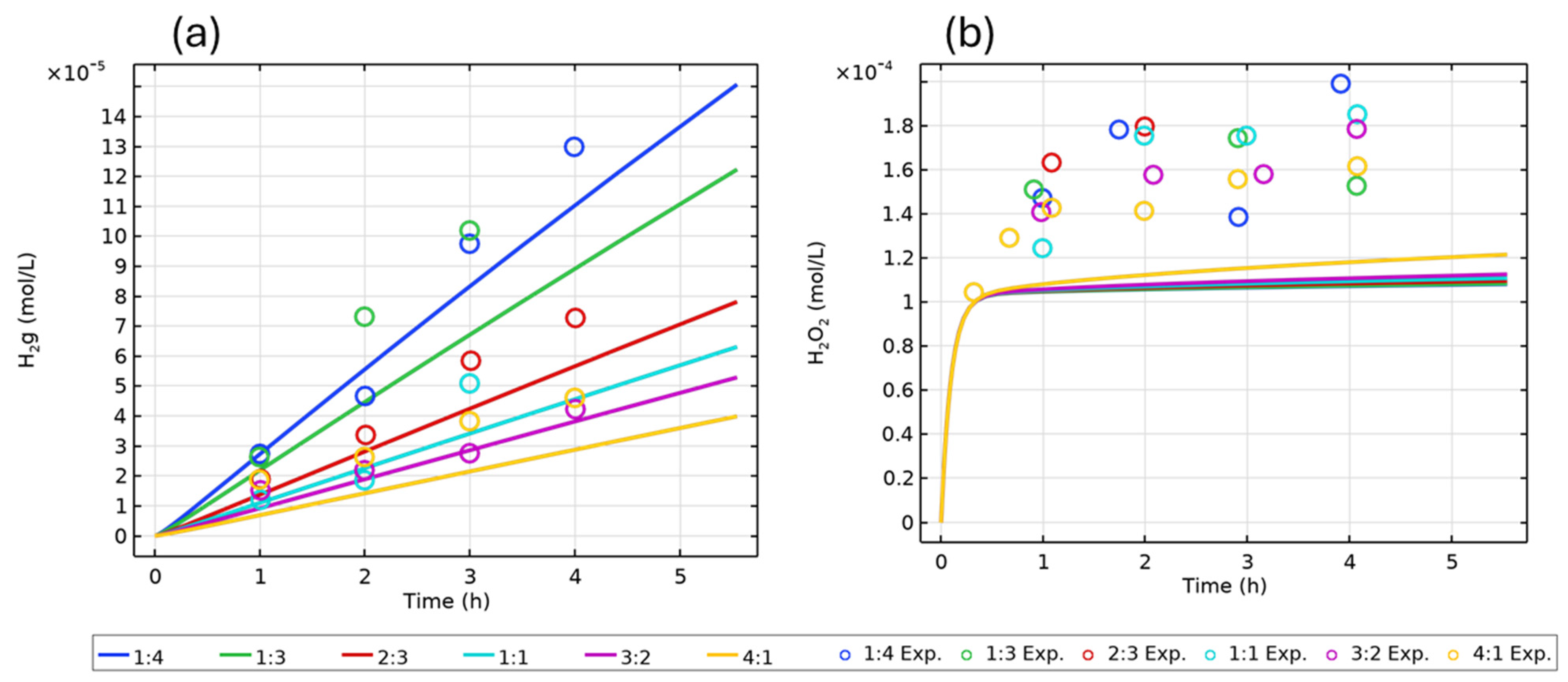
| 2 | H2O (COMSOL) | - | pH 6, aerated | Various | 9 | H2(g), H2O2(aq) [16] |
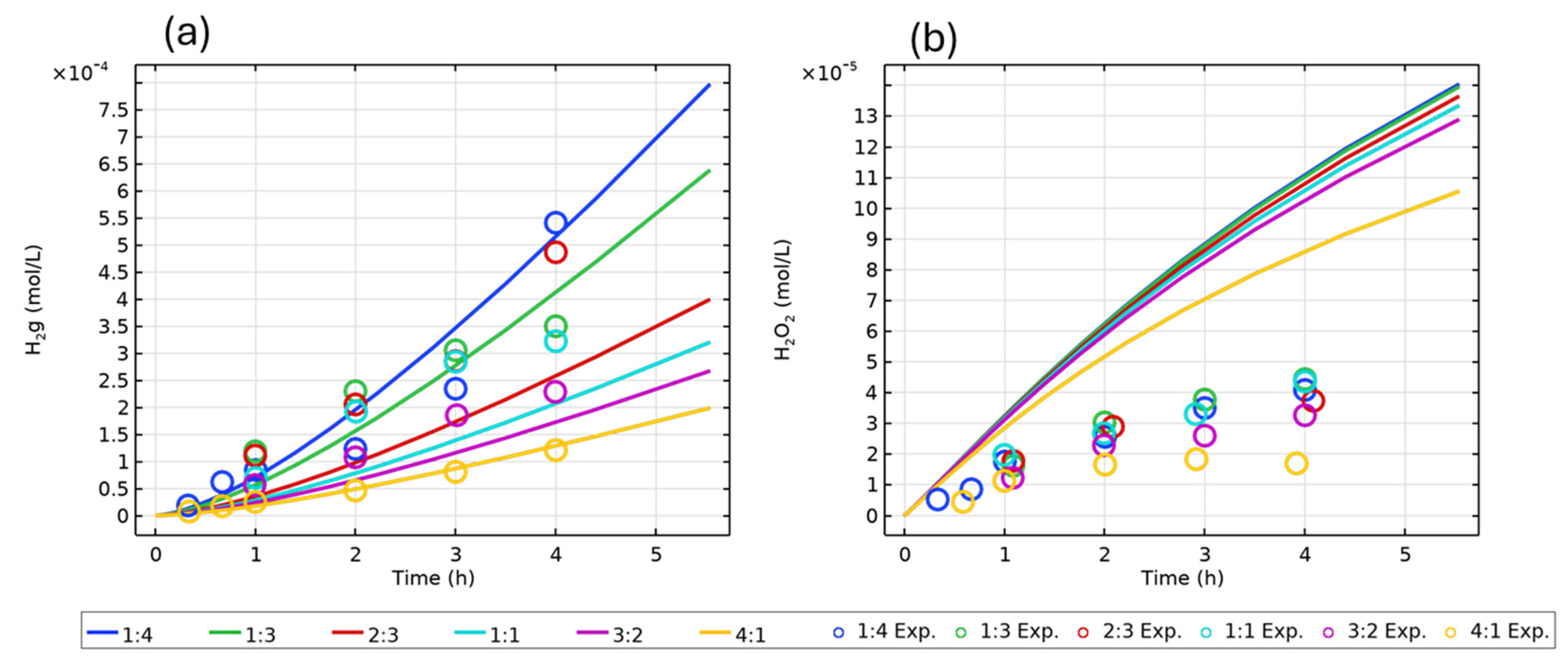
| 3 | H2O (COMSOL) | - | pH 10.6, deaerated | Various | 9 | H2(g), H2O2(aq) [16] |
| 5 | Morco Cl− (COMSOL) Jonsson Cl− (COMSOL) Morco Cl− (FACSIMILE) | 0, 0.001, 0.01 | pH 6, aerated | 1:1 | 2.3 | H2(g), H2O2(aq) [10] |
| 6 | Morco Cl− (COMSOL) Jonsson Cl− (COMSOL) Morco Cl− (FACSIMILE) | 2 | pH 7, aerated and “low [O2]” | 1:1 | 3 | H2(g), H2O2(aq) [10] |
Disclaimer/Publisher’s Note: The statements, opinions and data contained in all publications are solely those of the individual author(s) and contributor(s) and not of MDPI and/or the editor(s). MDPI and/or the editor(s) disclaim responsibility for any injury to people or property resulting from any ideas, methods, instructions or products referred to in the content. |
© 2025 by the authors. Licensee MDPI, Basel, Switzerland. This article is an open access article distributed under the terms and conditions of the Creative Commons Attribution (CC BY) license (https://creativecommons.org/licenses/by/4.0/).
Share and Cite
Briggs, S.; Behazin, M.; King, F. Validation of Water Radiolysis Models Against Experimental Data in Support of the Prediction of the Radiation-Induced Corrosion of Copper-Coated Used Fuel Containers. Corros. Mater. Degrad. 2025, 6, 14. https://doi.org/10.3390/cmd6020014
Briggs S, Behazin M, King F. Validation of Water Radiolysis Models Against Experimental Data in Support of the Prediction of the Radiation-Induced Corrosion of Copper-Coated Used Fuel Containers. Corrosion and Materials Degradation. 2025; 6(2):14. https://doi.org/10.3390/cmd6020014
Chicago/Turabian StyleBriggs, Scott, Mehran Behazin, and Fraser King. 2025. "Validation of Water Radiolysis Models Against Experimental Data in Support of the Prediction of the Radiation-Induced Corrosion of Copper-Coated Used Fuel Containers" Corrosion and Materials Degradation 6, no. 2: 14. https://doi.org/10.3390/cmd6020014
APA StyleBriggs, S., Behazin, M., & King, F. (2025). Validation of Water Radiolysis Models Against Experimental Data in Support of the Prediction of the Radiation-Induced Corrosion of Copper-Coated Used Fuel Containers. Corrosion and Materials Degradation, 6(2), 14. https://doi.org/10.3390/cmd6020014