Article

A Comparison of Different Natural Groundwaters from Repository Sites—Corrosivity, Chemistry and Microbial Community

1
Materials in Extreme Environments, VTT Technical Research Centre of Finland Ltd., 02150 Espoo, Finland
2
Process Microbiology and Food Safety, VTT Technical Research Centre of Finland Ltd., 02150 Espoo, Finland
3
Metals and Materials Recovery, VTT Technical Research Centre of Finland Ltd., 02150 Espoo, Finland
*
Author to whom correspondence should be addressed.
Corros. Mater. Degrad. 2021, 2(4), 603-624; https://doi.org/10.3390/cmd2040032
Submission received: 31 August 2021 / Revised: 13 October 2021 / Accepted: 14 October 2021 / Published: 21 October 2021

Abstract

:
In Finland, the repositories for low and intermediate-level radioactive waste (LLW and ILW) will be situated at three different geographical locations in about 60 to 100 m deep granite bedrock where the waste and waste containers can be subjected to anoxic groundwater containing microbes. The composition of groundwater varies in terms of chemistry and microbial activity in different locations. In this study, groundwater from the three repository areas was analyzed in respect to chemistry and microbial community. Corrosion tendency of three steel grades, carbon steel AISI/SAE 1005 and stainless steels AISI 304 and 316L, was studied in these groundwater environments using electrochemical methods. As a reference, measurements were also performed in simulated groundwater without microbes. The measurements show that corrosivity of the water and thus the steels’ performance differs depending on water origin. In addition, the groundwater differed remarkably in their chemical composition as well as abundance and diversity of microbial community between the sites. Consequently, the local environment has to be considered when evaluating the long-term evolution of disposal concepts.

1. Introduction

In Finland, the repositories for low- and intermediate-level radioactive waste (LLW and ILW) are or are planned to be situated in deep bedrock in the vicinity of the nuclear power plants. The facilities are excavated into crystalline bedrock about 60 m to 100 m below the ground level. The low- and intermediate-level waste will be packed into carbon steel containers in some of the concepts and especially the decommissioning waste itself contains both carbon steel and stainless steel. The repository time will be hundreds of years, and both the steel containers and the waste will be exposed to anoxic groundwater that contains naturally occurring microorganisms. These microorganisms are known to induce corrosion of steel materials [1,2]. Probably the most well-known group of microorganisms inducing steel corrosion under anoxic conditions are sulphate reducing bacteria (SRB) [3]. The types and amounts of microorganisms present in the repository environment depend on the physicochemical conditions of the bedrock and groundwater, i.e., temperature, pH, oxic/anoxic state, nutrient and trace element availability, electron donors and acceptors. Furthermore, microorganisms in deep bedrock are known to adjust their metabolism between, e.g., respiration and fermentation. For example, if sulphate runs scarce, many SRB may turn to fermentation of organic substrates [4].
Microorganisms are omnipresent in natural water. The size of the microbial communities in groundwater can be estimated by enumerating taxonomical marker genes, such as the bacterial 16S rRNA genes. In groundwater to the depth of 100 m, the number of bacterial 16S rRNA genes is estimated to be 105–106 copies mL−1 [5,6].
In this study, chemical composition and microbiology of natural groundwater from the three repository sites (two operating sites and one potential site) and one simulated groundwater experiment were determined. Additionally, corrosion properties of one carbon steel and two stainless steel types were studied by electrochemical measurements in these waters. Both sulphate and chloride are known to accelerate corrosion of steel, but for stainless steel, sulphate inhibits the pitting effect of chlorides if the sulphate/chloride ratio is high enough [7]. The inhibition effect of SO42−/Cl ratio increases with increased Cl concentration and temperature. However, in the case of higher alloyed steel grades, the effect is smaller than for low-alloyed steel grades. In measurements lasting only some hours, the microbes were assumed to not have adequate time to form biofilms or alter the surface conditions in other ways, and thus the chemical composition of the water was expected to be the main factor affecting the corrosion of steel. However, in the long term, microbes are believed to potentially have great impact to corrosion mechanisms of steels [1,8].

2. Materials and Methods

2.1. Steel Materials

Cold-rolled low carbon steel AISI 1005 (UNS G10050), and two stainless steels similar to AISI 304 (UNS S30400) and AISI 316L (UNS S31603) were studied in laboratory in anoxic conditions in three different natural groundwaters collected from three sites within Finland, named A, B and C. In addition, tests were performed also in one simplified simulated groundwater with chloride and sulphate contents similar to site C. The chemical compositions of the steels are presented in Table 1.
The test specimens were 10 mm × 10 mm coupons equipped with electrical contact via a wire joined at the back of the coupons. The back and the edges of the coupons were masked by epoxy-tar paint (Teknotar 100, Teknos) leaving an exposed surface area of 1 cm2 (grit 600). Before and after measurement, the specimens were rinsed with ethanol (96%) and air-dried. After the measurement, they were also photographed and stored in a dry atmosphere.

2.2. Water Chemistry

The natural groundwater samples were collected directly into oxygen free bottles from the drillholes and stored at 10°C until use. The simulated groundwater was prepared by adding 5500 mg/L chlorides (NaCl) and 500 mL/L sulphates (Na2SO4) to distilled water. The pH was adjusted to 7 using NaOH or HCl.
The measurements were performed in laboratory. Before the measurement, the electrolyte (300 mL) was purged to oxygen free using argon gas for 30 min.
Water chemistry analyses were conducted by ALS Finland using standardized methods. Shortly, pH using pH in water by the electrometric method [9], alkalinity, CO2/HCO3 based on alkalinity or acidity, spectrometric [10], ammonium spectrometric detection [11], Ca, Mg, Na, S, Si using ICP-OES [12] and TOC [13].
The Langelier saturation index was calculated as described in [14]. The pitting index was calculated based on the salinity and alkalinity of the water. If the oxygen content of the water is low, i.e., c(O2) < 0.1 g/m, no protective layer is formed on the steel, and the surface can suffer from pitting and other localized corrosion (Standard DIN 50 930 Teil 2, 1993).
Probability of local corrosion is decreased when
[c(Cl) + 2c(SO42−)]/c(HCO3) < 1
where
  • c(Cl) The chloride concentration (mol/m3)
  • c(SO42−) The sulphate concentration (mol/m3)
  • c(HCO3) The bicarbonate concentration (mol/m3).

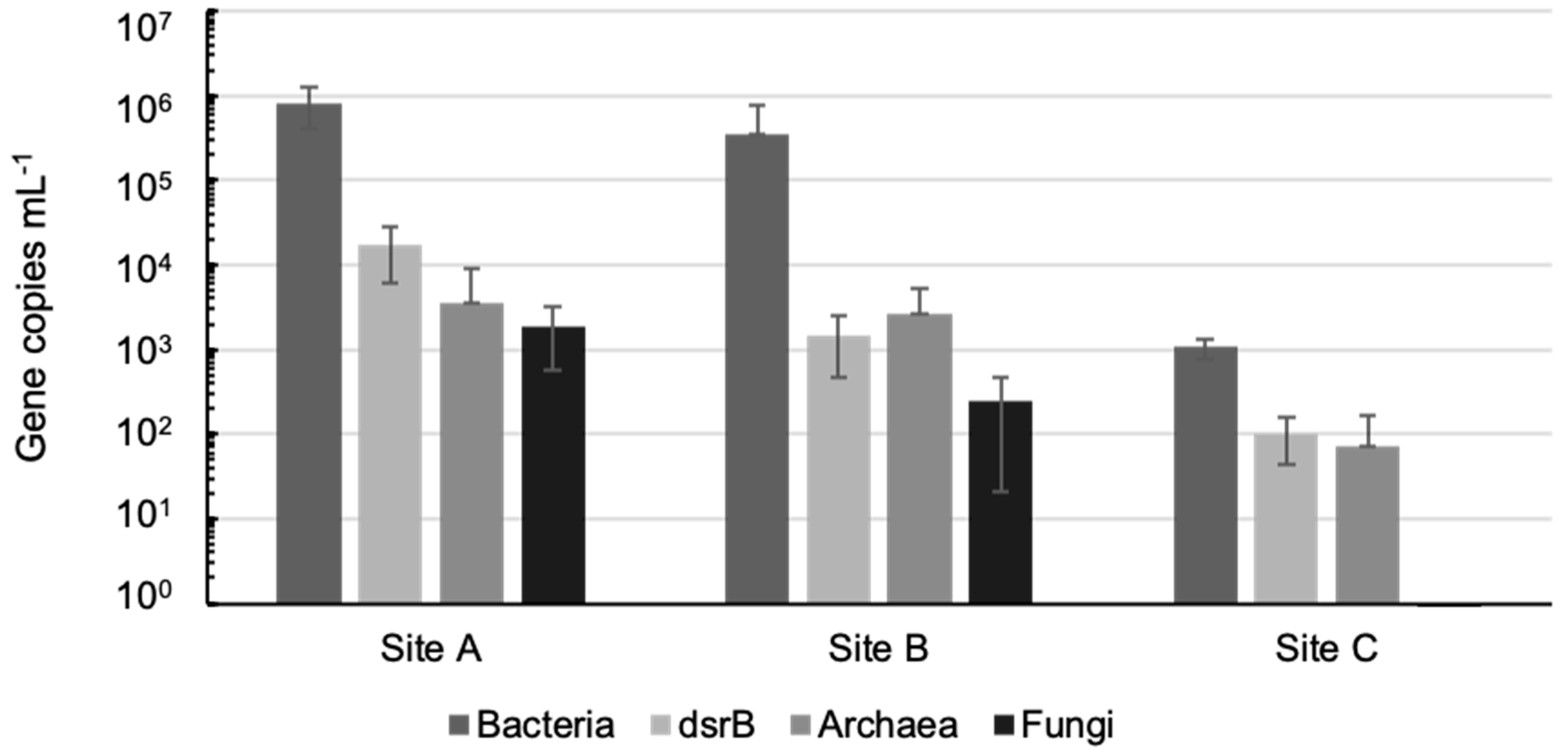
2.3. Estimation of Microbial Community Sizes in the Different Groundwaters by qPCR

The microbial biomass from duplicate groundwater samples (each 0.5 L site A or 1 L Sites B and C) was collected on 0.2 µm pore-size cellulose acetate membranes (Corning) by vacuum suction. The water was filtered in a laminar flow hood, and the membranes were cut out of the filtration units immediately after filtration and frozen at −20 °C until DNA extraction. For extraction of DNA, the filters were briefly thawed on ice and placed into sterile 5 mL Eppendorf tubes using sterile tweezers. The DNA was extracted from the thawed filters with the NucleoSpin® Soil DNA extraction kit (Macherey-Nagel, Düren, Germany). The beads from two bead tubes (provided in the kit) were added on top of the filters, and the DNA was extracted using double volumes of lysis buffer SL1 and enhancer solution SX. The tubes were placed horizontally on a vortex genie 2.0 shaker (full speed) for 5 min. Contaminants were removed from the lysate with double volumes of buffer SL3 and a 5 min incubation at +4 °C before a 1 min centrifugation at 11.000 g. The lysate was filtered on the NucleoSpin® (Macherey-Nagel, Düren, Germany) inhibitor removal column, where after the DNA in the lysate was bound on the NucleoSpin® soil DNA-binding column. The DNA was purified according to the manufacturer’s instructions, and the DNA was eluted in 100 µL of buffer SE.
Quantitative PCR (qPCR) targeting the bacterial and archaeal 16S rRNA genes, fungal 5.8S rRNA genes and the dsrB genes in sulphate reducers were used as a proxy for community size. The qPCR approach was chosen instead of direct microscopy, since it is not possible to distinguish between bacteria in general, sulphate reducers, archaea or fungi by microscopy, and the qPCR is an established technique for unbiased comparison of samples from different sites. Thus, the number of bacteria, archaea, fungi and sulphate reducing bacteria was estimated using quantitative PCR (qPCR). The bacteria were targeted with the S-D-Bact-0341-b-S-17/S-D-Bact-0785-a-A-21 primers [15] targeting the bacterial 16S rRNA genes and the dsrB genes of the SRB were detected with the DSRp2060F and DSR4 primers [16,17]. The reaction mixture contained 1× SensiFAST SYBR No-ROX master mix for LightCycler480 (Bioline, London, UK), 2.5 mM of forward and reverse primer, 1 µL DNA extract, DNA standard or water, and was topped to 10 µL with nuclease-free water. The amplification consisted of an initial denaturation step of 15 min at 95 °C, followed by 30 and 45 amplification cycles for bacterial 16S rRNA genes and dsrB genes, respectively. The amplification cycles consisted of denaturation for 10 s at 95 °C, annealing of primers for 35 s at 57 °C and 55 °C, respectively, and an elongation step for 30 s at 72 °C. The fluorescence in the samples was measured at the end of each elongation step. A final elongation step of 3 min at 72 °C followed the amplification cycles and was further followed by a melting curve analysis. The melting curve analysis step consisted of denaturation for 10 s at 95 °C, annealing of the strands for 1 min at 65 °C and gradual temperature increase (20 °C s−1) to 95 °C, with continuous fluorescence measurement.
The archaea were targeted with primers A344F [18] and A744R [19] for the archaeal 16S rRNA gene and detected with the FAM-labelled probe A516F [20] as described in [21]. Fungal 5.8S rRNA genes were targeted with the primers 5.8F1 and 5.8R1 and detected with FAM-labeled 5.8P probe [22]. The qPCR was run in triplicate reactions for each replicate sample. The reaction mixture contained 1× SensiFAST Probe No-ROX master mix, 0.5 μM forward and reverse primers, 0.2 μM probe and nuclease-free water to 10 µL. The qPCR programme consisted of an initial denaturation and polymerase activation step of 3 min at 95 °C, followed by 40 cycles of 10 s at 95 °C, 30 s at 62 °C and 1 s at 72 °C.
The qPCR analyses were performed with a LightCycler 480 (Roche Applied Science) using triplicate 10 µL reactions for each replicate sample. The amplification results were compared to known standard dilution series consisting of a plasmid containing the 16S rRNA gene of Escherichia coli for bacteria and Halobacterium salinarum for archaea, the 5.8S rRNA gene of Aspergillus versicolor for fungi and the dsrB gene of Desulfovibrio desulfuricans for the SRB.
The bacterial, archaeal and fungal community composition of the groundwater samples from sites A, B and C were characterized using high throughput amplicon sequencing of the bacterial and archaeal 16S rRNA genes and the fungal ITS1 region. The bacterial and archaeal v3v4 region of the 16S rRNA gene was targeted using Bact_0341F/Bact_805R [15] and S-D-Arch-0349-a-S-17/S-D-Arch-0787-a-A-20 [23] primers, respectively. The fungal ITS1 region was amplified with primer pair ITS1 and ITS2 [24,25]. The amplicon libraries were prepared in parallel 25 µL PCR reactions using the 2× MyTaqTM Red Mix (Bioline, London, UK). The reactions contained 800 nM of forward and reverse primers and 2 μL DNA template. The PCR program consisted of an initial 3 min denaturation step at 95 °C, 35 amplification cycles of 15 s at 95 °C, 15 s at 50 °C and 15 s at 72 °C, followed by a final 30 s step at 72 °C. The amplification success and correct size of the PCR products were verified with agarose gel electrophoresis before they were sent for sequencing on the Ion Torrent PGM platform at Bioser (Oulu, Finland). The amplicons were further purified and size-selected before sequencing by the staff at Bioser.
The sequence reads were analyzed using the Mothur software (v.1.41.3) [26] to remove adapter, barcode and primer sequences, and to exclude sequences that did not meet the quality criteria (no barcode mismatches, maximum two primer mismatches, no ambiguous nucleotides, maximum eight nucleotide long homopolymer stretches and a minimum length of 200 bp). A qwindowaverage of 25 and a qwindowsize of 50 were used on the PGM read data to remove erroneous reads from the data set.
The Silva seed database version 138 [27,28] was optimized to cover the same region as the amplicons using the pcr.seqs command in Mothur separately for bacteria and archaea. The bacterial and archaeal 16S rRNA sequences were aligned with Mothur to the modified Silva seed reference alignment. Chimeric sequence reads were removed with vsearch in Mothur, where after the dereplicated sequences were classified using the modified Silva seed reference alignment and taxonomy using a cutoff of 80. Sequences that were not classified as bacteria were removed from the bacterial sequence data, and sequences failing to be classified as archaea were removed from the archaeal sequence data. A distance matrix was calculated using the dist. seqs command in Mothur with default parameters. The filtered sequences were clustered into OTUs based on the distance matrix using vsearch dgc in Mothur and a cutoff of 0.03.
The fungal ITS sequence data was trimmed using the same quality parameters as for the bacterial and archaeal sequence data. The sequence data was dereplicated with unique.seqs, left un-aligned, and tested for chimeric sequences using the chimera.vsearch command. Non-chimeric sequences were classified with the classify.seqs command towards the Unite version 8 full ITS database. Non-fungal sequences were removed whereafter the sequences were clustered into OTUs with 97% sequence homology.
The microbial community data was analyzed with R (version 4.0.4) in RStudio [29] mainly with packages phyloseq [30] and vegan [31]. Taxonomy and ordination plots were visualized with packages ggplot2 and ampvis2 [32,33]. The Bray–Curtis dissimilarity model was used for principal coordinates analysis (PCoA). Alpha diversity measures for bacterial, archaeal and fungal communities were calculated from raw read data with the estimate-richness function from the phyloseq package.

2.4. Electrochemical Measurements

The electrochemical measurements were performed in a laboratory by using a three-electrode electrochemical cell in an anoxic environment (under Ar flow) at room temperature. The cell was a glass beaker covered with a parafilm and the volume of the electrolyte was 300 mL. Before the measurement the electrolyte was purged to oxygen free with Ar (about 200 mL/min) for 30 min. After the electrodes were placed in the cell, Ar purging was continued at a slower speed (about 70 mL/min) to maintain the anoxic conditions. The electrodes were situated vertically in the middle of the beaker and the purging pipe with filter was close to the beaker wall about behind the working electrode. The exposed surface of the working electrode was situated vertically and the specimen surface was faced about 2 cm distance to the graphite bar that was used as a counter electrode. The tip of the saturated Ag-AgCl reference electrode was situated close to the working electrode surface at the upper level of the working electrode. The potential values were measured with an Ag-AgCl reference electrode but converted to standard hydrogen electrode (SHE) scale after measurement. The replicate measurements (2–3) were performed using fresh batch of electrolyte (groundwater or simulated groundwater) and replicate specimens.
For carbon steel, the open circuit potential (OCP) was measured for one hour, and after that, Tafel curves were measured from −250 to +250 mV vs. OCP using replicate specimens. The scanning speed was 10 mV/min. Gamry Echem Analyst program was used to determine the corrosion current and the corrosion rate from the Tafel curves. The corrosion rate was calculated by equation
CR = IcorrKEW/dA
where
  • CR The corrosion rate. Its units are given by the choice of K
  • Icorr The corrosion current in amperes
  • K A constant that defines the units for the corrosion rate
  • EW The equivalent weight in grams/equivalent
  • d Density in grams/cm³
  • A Area of the sample in cm².
For stainless steels, OCP was measured at least for one hour. After OCP measurement, a cyclic polarization curve was measured by shifting the potential from OCP until the corrosion current reached 5 mA/cm2 or the voltage reached +1000 mV vs Ag-AgCl. The scanning rate was 18 mV/min.
After the measurement, the specimen was studied under a stereomicroscope to verify the type and amount of corrosion. Each specimen was photographed, and then the selected specimens were examined closely by a scanning electron microscope (SEM).

3. Results

3.1. Chemical Composition and Physical Properties of the Groundwaters

In the groundwaters of different repository sites, there were significant differences in the chemical composition and parameters (Table 2). The chloride and sulphate contents in the groundwater from site C and the simulated groundwater were at the level of brackish water. However, they are significantly lower in the groundwaters from sites A and B. The amounts of calcium (Ca), magnesium (Mg) and sodium (Na) correlate with the amounts of cations, e.g., chlorides and sulphates. The alkalinity, the total amount of carbon dioxide (CO2), bicarbonate (HCO3) and the total organic carbon (TOC) are the highest in the groundwater from site B and lowest in the groundwater from site C. In the groundwater of the site A the amount of ammonium is about a decade lower than in the groundwaters from sites B and C.
The pitting index values of the groundwaters are between 7 to 82, indicating the pitting tendency of carbon steel in the waters. A positive Langelier saturation index indicates the possible formation of a protective scale on a steel surface. In site C, the Langelier index is closest to the area where scale formation tendency is low.

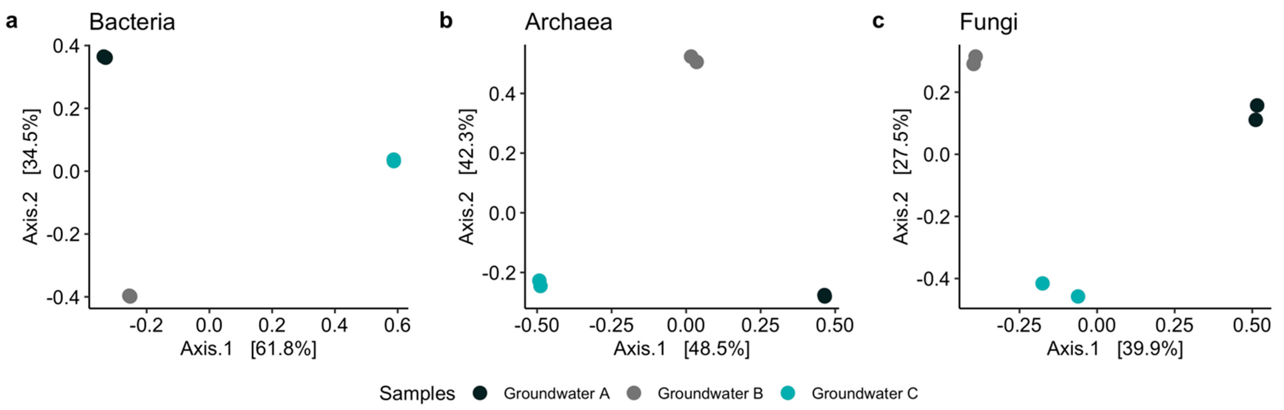
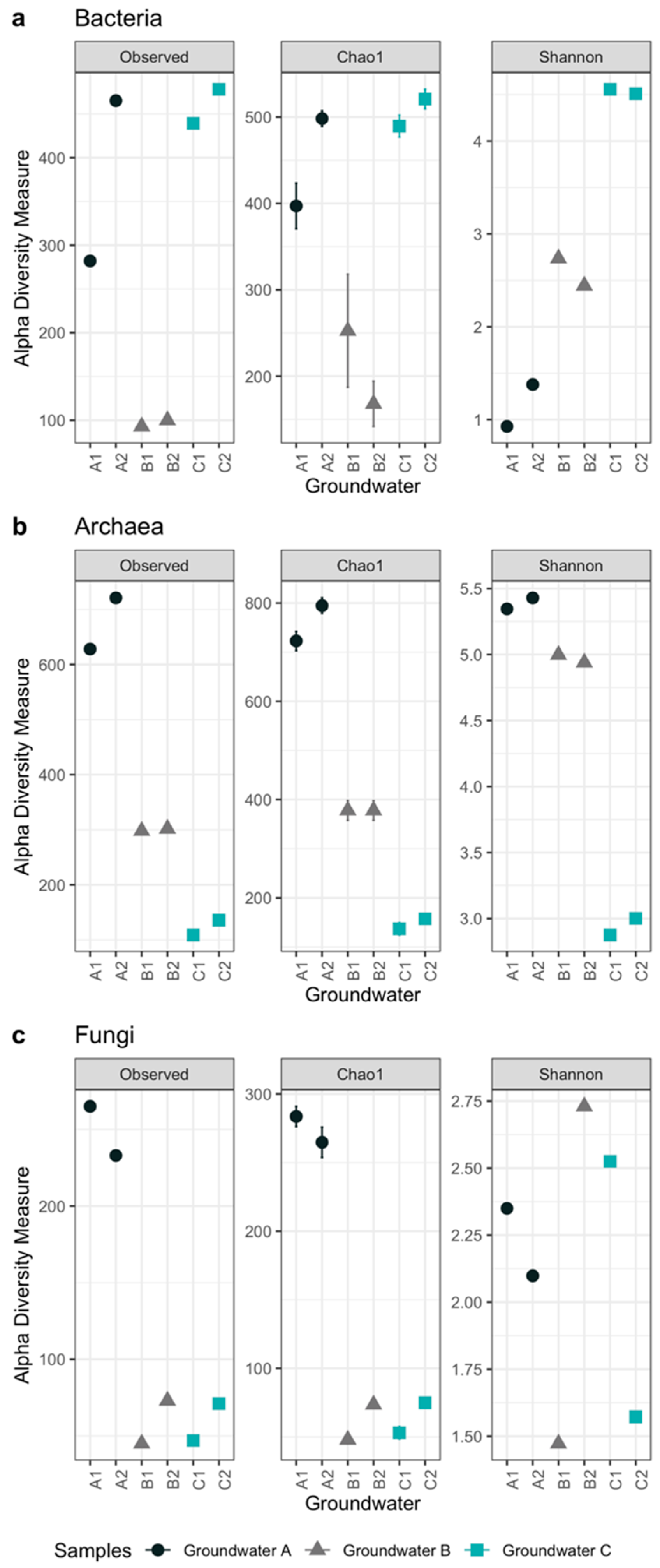
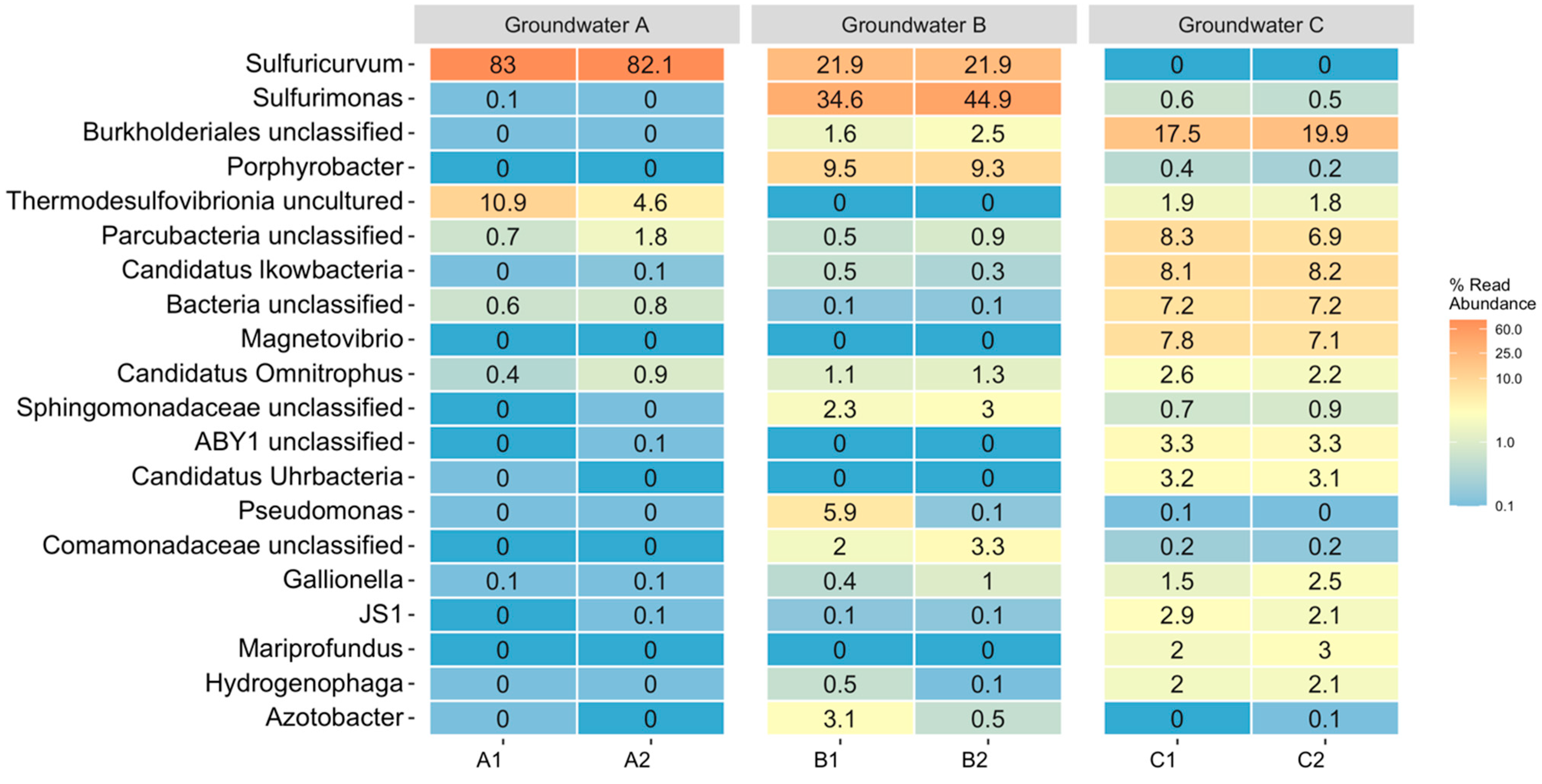
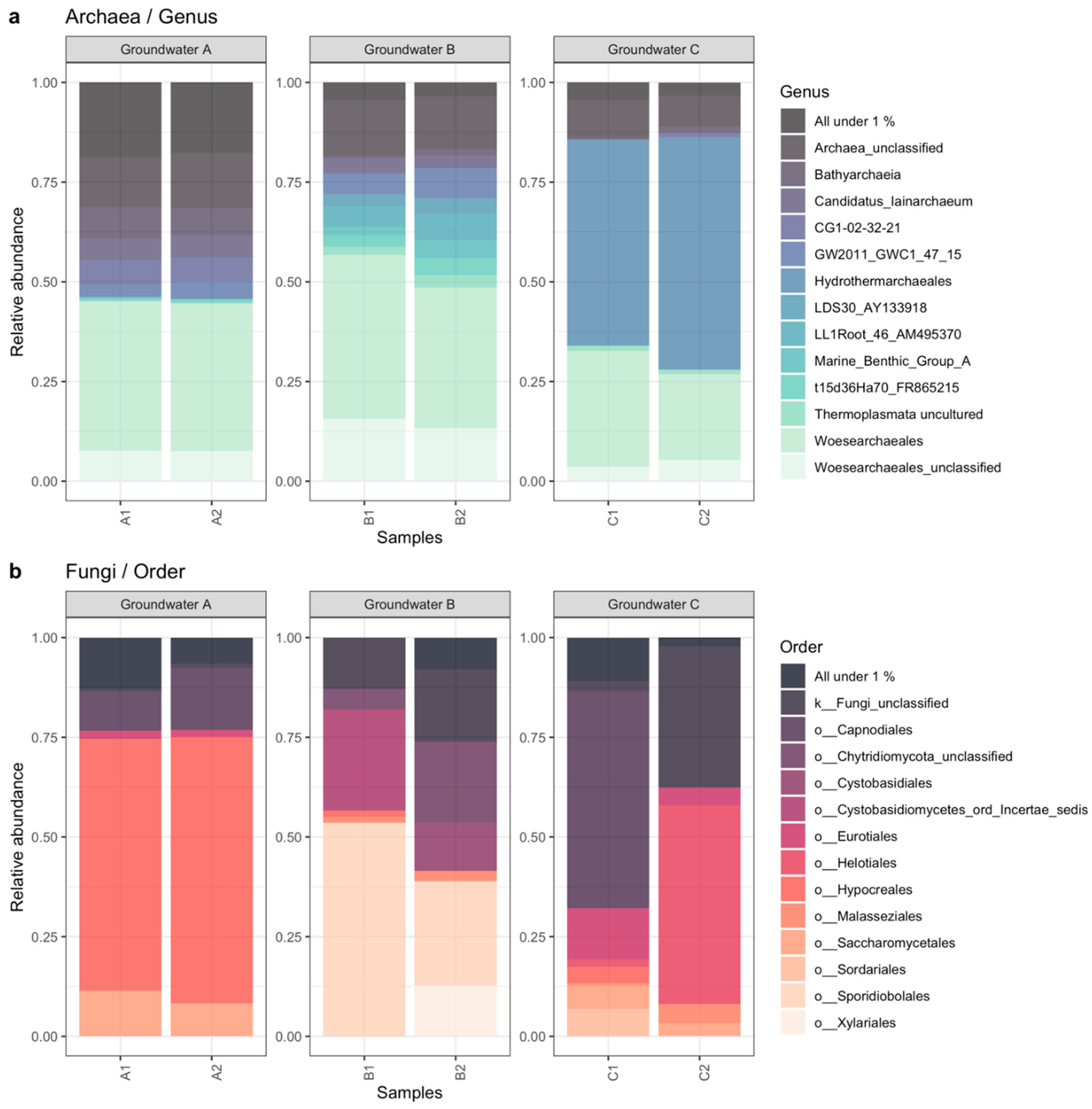
3.2. Microbiology of the Groundwaters

The amounts of bacteria, sulphate reducing bacteria (by dsrB gene copies), archaea and fungi per milliliter groundwater were determined from all test sites by qPCR (Figure 1). Bacteria were more abundant than archaea and fungi, and the highest numbers of 8.9 × 10⁵ and 3.5 × 10⁵ bacterial 16S rRNA gene copies mL−1 groundwater were detected in groundwaters from sites A and B, respectively, whereas groundwater from site C had only 5.0 × 10³ bacterial 16S rRNA gene copies mL−1. All groundwaters contained bacteria, sulphate reducing bacteria and archaea but only groundwaters from sites A and B contained adequate amounts of fungi that could be detected above the background noise of the assay. The SRB community detected by the dsrB gene was also more prominent in groundwaters from sites A and B, 1.7 × 10⁴ mL−1 and 1.5 × 10³ dsrB gene copies mL−1, respectively, whereas in groundwater from site C the number was below 102 copies mL−1. The number of archaeal 16S rRNA genes was 3.5 × 10³ and 2.7 × 10³ copies mL−1 in groundwaters from site A and B, respectively, but below 102 copies mL−1 in groundwater from site C. The number of fungal 5.8S rRNA gene copies was 1.9 × 10³ mL−1 and 2.5 × 10² mL−1 in groundwaters from sites A and B, respectively, but below the limit of detection in groundwater from site C.
The microbial communities in the different groundwater types and locations were clearly different from each other (Figure 2). This was clearly seen in the principal coordinates analysis (PCoA), where the replicate samples from the same site grouped closely together according to the bacterial, archaeal and fungal community composition, but were situated far from each other on the PCoA plots.
The bacterial community with the highest OTU richness, i.e., number of observed operational taxonomic units (OTUs) and estimated number of bacterial OTUs (Chao1) was found in groundwaters from sites A and C, whereas groundwater from site B showed the lowest bacterial community richness. The highest diversity index (Shannon) was found in site C, and lowest at site A (Figure 3, Table 3).
In contrast, the highest archaeal OTU richness and diversity index was observed in the groundwater from site A and the lowest in groundwater from site C. The fungal communities also showed highest OTU richness in groundwater from site A, but only little differences were observed between groundwaters from sites B and C.
The bacterial, archaeal and fungal communities in two replicate samples of groundwaters from all sites were characterized using high throughput amplicon sequencing. In groundwater from site A, motile sulphur-oxidizing bacteria belonging to the genus Sulfuricurvum dominated the community contributing with >78% of the sequence reads (Figure 4). Groundwater from site B had also a high relative abundance of Sulfuricurvum (up to 21.9%) but the dominating bacterial genus in groundwater from site B was the Sulfurimonas (34.6–44.9%). The bacterial community in groundwater from site C differed significantly from that of groundwater from sites A and B (Figure 2a). The most prominent bacterial group belonged to so far undetermined Burkholderiales bacteria, which contributed with 18.6–21.0% of the bacterial community in the groundwater from site C. In addition, approximately 7.1% of the bacterial sequence reads belonged to the genus Magnetovibrio. Groundwater from site C also contained a substantial proportion of small cell-size, symbiotic bacteria belonging to the candidate phylum Parcubacteria (7.6% of the bacterial community) and candidate order Falkowbacteria (7.6% of the bacterial community).
The archaeal communities differed between the sites (Figure 2b). Woesearchaeales represented between 24.5% and 56.0% of the archaeal communities in the different sites and were the most common archaea in groundwaters from sites A and B (Figure 5a). In groundwater from site C, up to 58.6% of the archaeal community consisted of Hydrothermarchaeales, which were absent in groundwaters from sites A and B.
The majority of the fungi detected in groundwater from site A belonged to the Ascomycota division (Figure 5b). The dominating fungal family was the Hypocreales (62.5–66.5% of the fungal community), and Saccharomycetales and Capnodiales contributed with 8.2–11.4% and 9.7–15.5%, respectively. In contrast, groundwater from site B contained fungi belonging to the Basidiomycetes division, with Sporidiobolales contributing with 24.7–51.8% of the fungal community. The Chytridiomycetes division was represented by 5.0–19.0% of the fungal community in groundwater from site B and between 15.7–22.8% of the fungal sequences belonged to unclassified or unknown fungal groups. In groundwater from site C, Saccharomycetales contributed with 20.8–67.9% of the fungal sequence reads, whereas up to 16.3% belonged to Sporidiobolales, 31.4% to Chytridiomycetes and 29.2% to unclassified fungal groups.

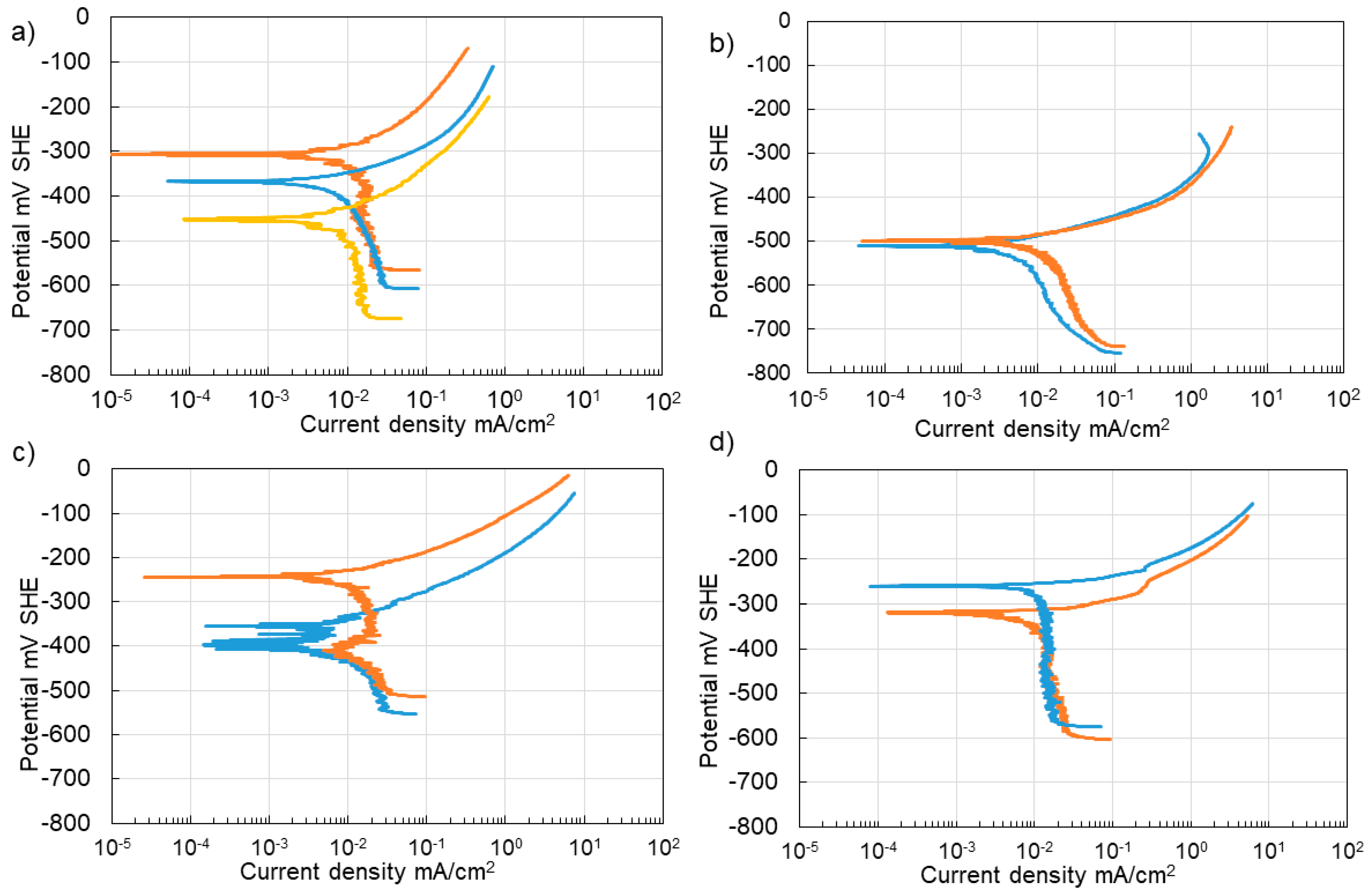
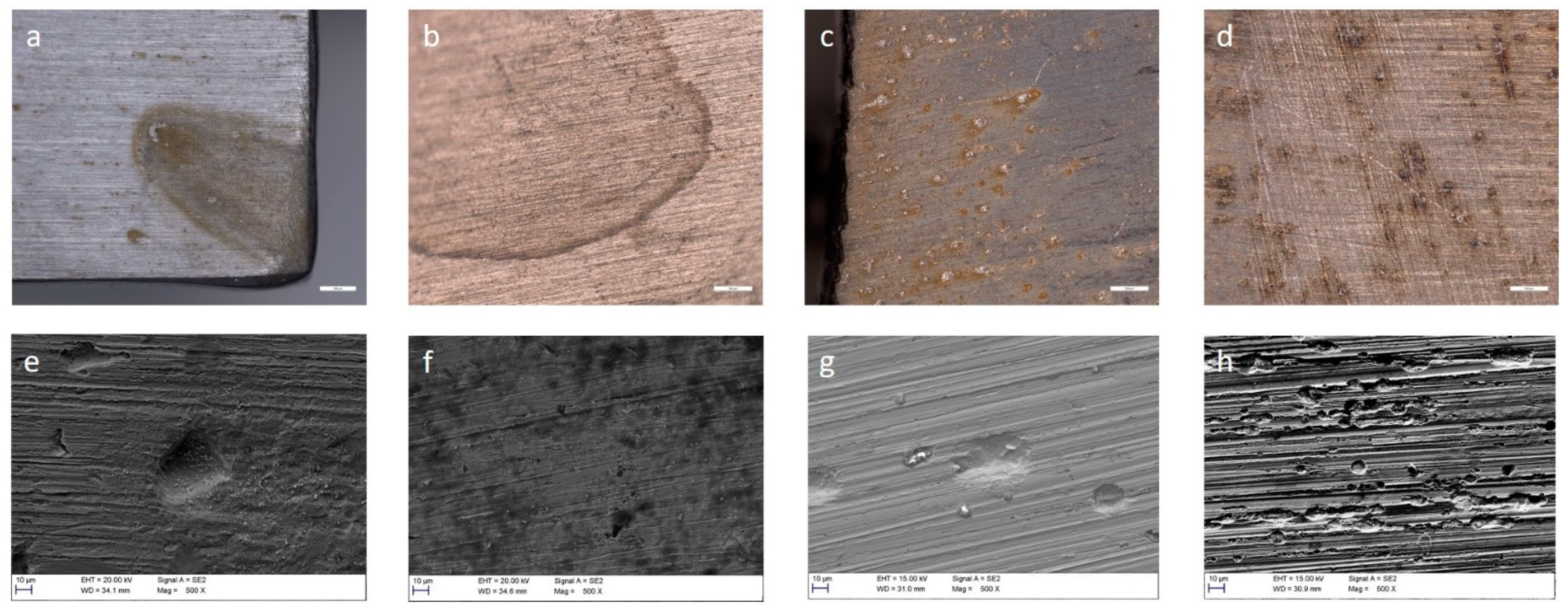
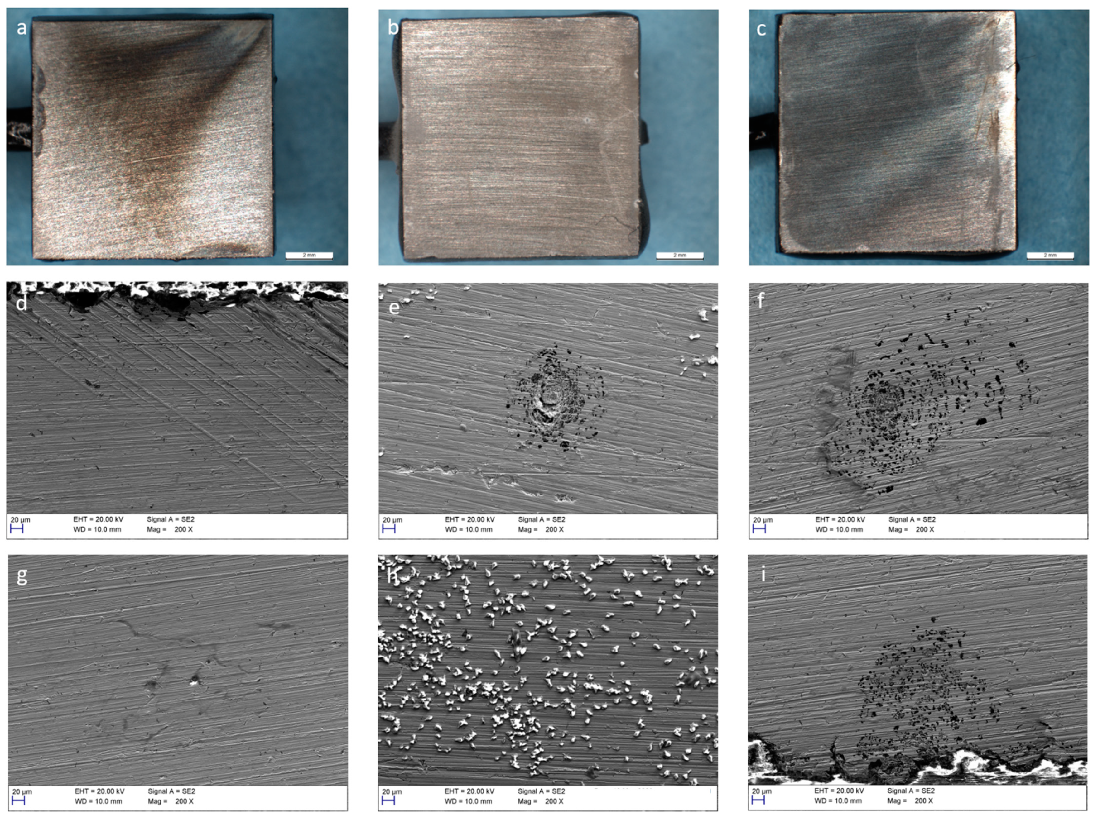
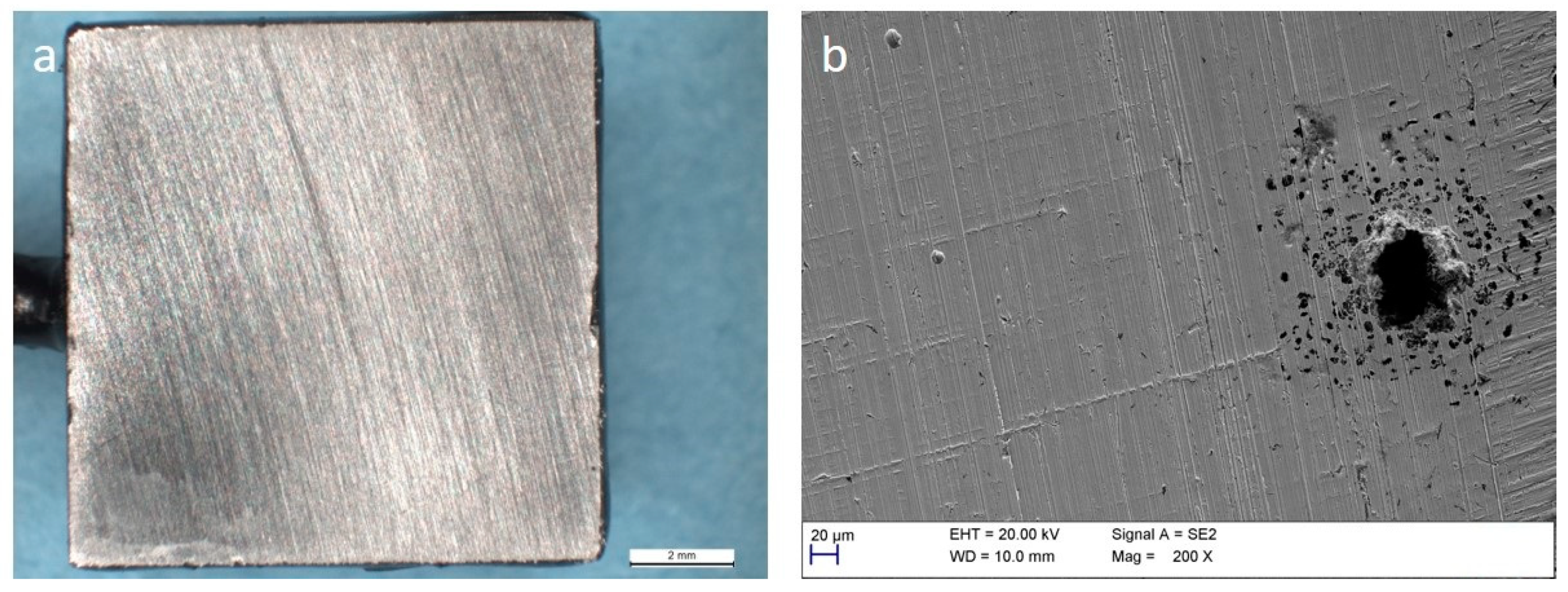
3.3. Corrosion of Carbon Steel

In most of the replicate measurements, the open circuit potential (OCP) measured before the polarization and the corrosion potential (Ecorr) determined from the polarization curves in Figure 6 were about ±30 mV to each other. That was expected due to the effect of polarization on corrosion potential. However, in the curves measured in groundwater from site C, the Ecorr in Figure 6c was even 100 mV lower than the OCP determined before the polarization. The curves measured with replicate specimens in groundwater from site B showed the lowest OCP and Ecorr and the parallel curves were almost alike (Figure 6b). There was more scatter between the curves measured in the other groundwaters. Differences between the curves of the replicate specimens indicated that there were also differences in corrosion behavior.
Due to complex shape of some polarization curves, the used software could not determine the corrosion current in each case. Therefore, icorr was determined manually from the polarization curves in Figure 6 by extrapolating the linear part of only the cathodic curve to the corrosion potential Ecorr. Because the Tafel curves of the replicate specimens were not identical, there was deviation in the average corrosion rates determined from the curves (Figure 7). As was expected based on the Tafel curves and corrosion potentials, groundwater from sites A and C had the highest deviation in corrosion rates. The lowest average corrosion rate, although with significant deviation, was measured in groundwater from site C, whereas the highest corrosion rates were measured in the simulated groundwater.
The calculated pitting index values predicted pitting of carbon steel in all natural groundwaters. All specimens used in polarization measurements were further studied visually and with microscopy. The specimens measured in groundwaters from sites A and C and the simulated groundwater contained mostly localized corrosion (Figure 8a,c,d). In contrast, no regular-shaped corrosion pits were found on the specimens measured in groundwater from site B, and the corrosion appeared to be more general (Figure 8b).
The surface of the specimen measured in the simulated groundwater was covered by microscopic pits (Figure 8h) whereas the specimens tested in groundwaters from sites A (Figure 8e) and C (Figure 8g) had fewer and larger pits. The pit in Figure 8e is in the middle area shown in Figure 8a. The specimen was situated in the cell vertically, and the right side of picture was situated towards to the beaker bottom. The iron ions have diffused out of the pit and formed the colorful iron oxides on the surface. The flowing of the electrolyte due to purging causes the corrosion products to be not directly below the pit.

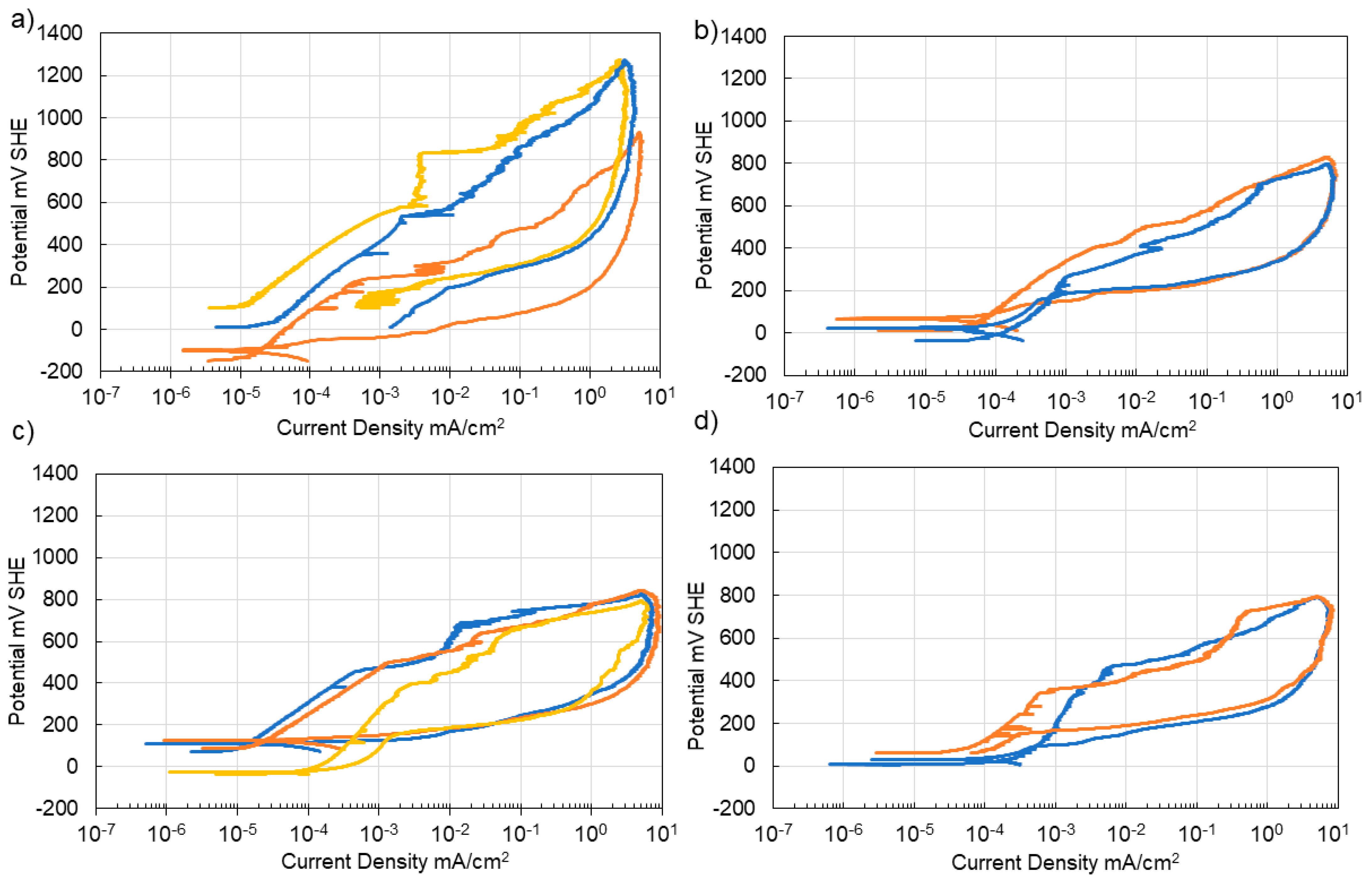
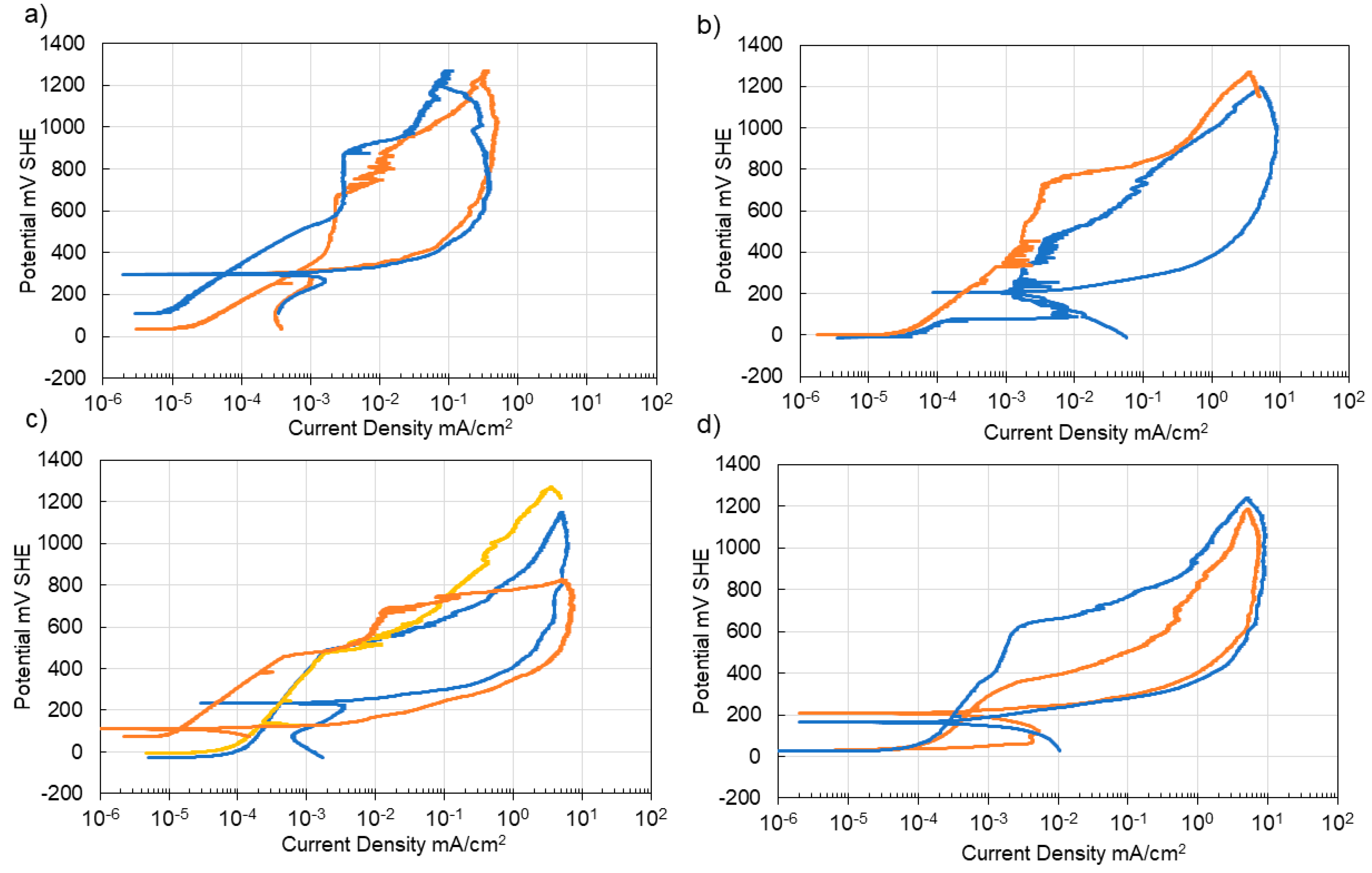
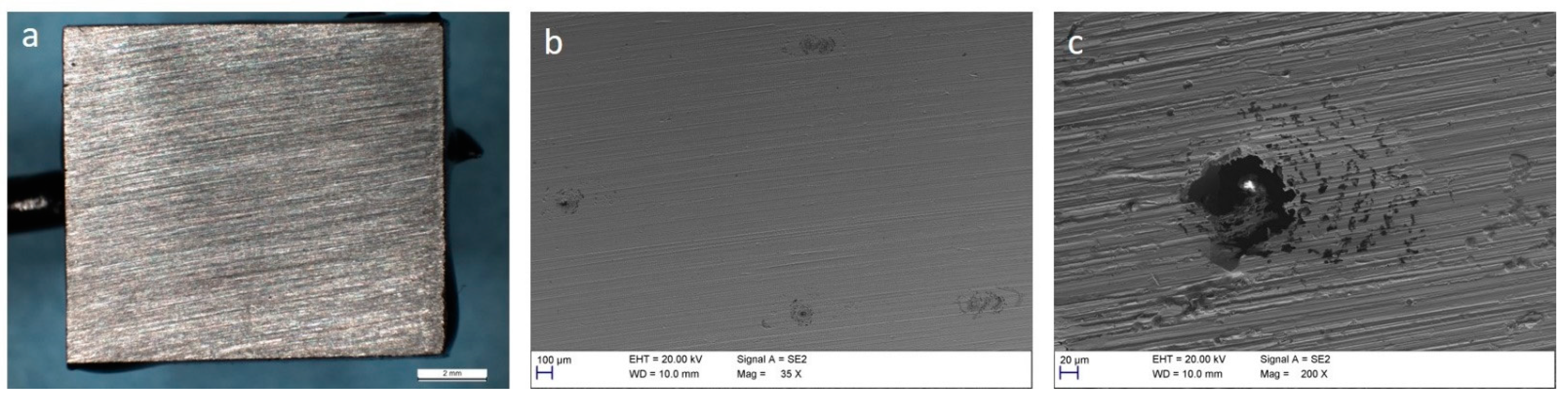
3.4. Corrosion of Stainless Steel

The average values of the open circuit potentials (OCP), the pit nucleation potentials (Epn) and the pit re-passivation potentials (Epp) of replicate specimens of steel 304 were quite close to each other (Figure 9) except in one curve measured in groundwater from site A (Figure 9a). For steel 316L, there was more variety in the shape of the curves (Figure 10). For both steels, most of the curves are closed which indicates that pits passivate, and possible crevice corrosion also ceases when the potential is reduced back to the OCP.
There was variation in the OCPs, the pitting and re-passivation potentials due to differences in curves between the replicate specimens (Figure 11). In some curves, e.g., steel 304 in groundwater from site B (Figure 9b), no real passivation region is seen which indicates that crevice corrosion starts immediately. Crevice corrosion was proved by visual inspection and a stereomicroscope.
In all AISI 304 steel specimens tested in cyclic polarization in natural groundwater, the surface turns darker (Figure 12a–c). However, there are local light areas around pits and near the edge where crevice corrosion is seen. Some of the pits are wholly or partly covered with a lacy cover (Figure 12e,f) but also in the open pits have signs that they have had similar covers (Figure 11d). In the specimens of steel 304 measured in simulated groundwater, the surface is light, and only a few pits or a little crevice corrosion are to see by a stereomicroscope (Figure 13a). However, in the inspection by SEM, it can be seen that there are lots of covered pits on the surface, although there are no corrosion products to indicate it (Figure 13b,c).
In the specimens of steel 316L exposed to the natural groundwaters, the most severe corrosion is between the edges and the protective paint (Figure 14a–d,i). On the surfaces, there are only a few pits (Figure 14e,f), and they are covered alike in the case of steel 304. Corrosion products are seen on the surfaces of the specimens studied in natural groundwaters from sites A, B and C (Figure 14a–c). Inspection by SEM indicate crevice corrosion between the steel and the protective paints (Figure 14d) or covered pits (Figure 14e,f). On the surface of the specimen exposed to the simulated groundwater, there is no visible corrosion products (Figure 15a) but a few partially covered pits are seen by SEM (Figure 15b).

4. Discussion

High chloride concentrations are known to affect localized corrosion of steels. In the present study, this is supported by the observation, that the localized corrosion was detected in electrochemical experiments on all steel grades included. Both the electrochemical results and the visual inspection of the steel specimens indicated that there might have been variation between the replicate measurements or in the experimental conditions of the replicate specimens.
The surface of the carbon steel specimens measured in the simulated groundwater with high chloride content were covered by microscopic pits and the highest corrosion rate were determined for those specimens. The simulated groundwater contained only chloride, sulphate and sodium additions. The buffering substances were lacking from this environment explaining the highest corrosion rates detected.
There were occasional large pits on the specimens exposed to the groundwater from site C, but also in specimens measured in groundwater from site A where the chloride content was remarkably lower. However, in groundwater from site B the corrosion of carbon steel was rather general than localized although the chloride concentration was close to that of the groundwater from site C and the simulated groundwater.
In the natural groundwaters, the highest chloride concentrations in groundwater from site C resulted in the lowest corrosion rate of carbon steel. This indicates that chlorides were not the only species that affected corrosion. Additionally, in groundwater from site C the alkalinity, the total amount of carbon dioxide, bicarbonate concentration and the total amount of organic carbon were the lowest. The corrosion rate of carbon steel in anoxic and alkaline water should remain slow [14], further raising the question of the mechanism driving the corrosion under the conditions studied. The differences between the average corrosion rates in groundwaters from sites A, B and C might be associated with the differences in Ca hardness, which is the lowest in site A and highest in site C. Additionally, the groundwater in site A had the highest analyzed sulphide level, while the sulphide content of groundwaters from other sites was below the limit of quantification. Furthermore, there are differences in organic carbon content in these groundwaters. In waters containing organic substances or colloidal silica, calcium carbonate may precipitate on these substances instead of the metal surface [14].
The chloride contents of groundwater from site C and simulated groundwater were similar to brackish water. All the groundwater tended to cause pitting in carbon steel, which is in line with the calculated pitting indexes. However, the pitting behavior of carbon steel differed in these waters, which indicated that high chloride and sulphate contents were not the only reasons for differences in the corrosion behavior of carbon steel. Low alkalinity and low Ca-hardness also are known to enhance corrosion. That indicates that there might be some inhibiting substances, such as nitrite, a known inhibitor, which was below the detection limit of the analysis. For stainless steel AISI 316L the pit initiation potential (Epn) and the pit passivation potential (Epp) decreased when the chloride concentration of the groundwater increased. However, for AISI 304 the correlation between potential and chloride concentration was not linear, although the highest potential values were measured in the groundwater from site A that had the lowest chloride concentration. The relations between the water composition and different parameters to the corrosion rate and form seem to be more complex. Therefore, the corrosion behavior of the steel cannot be predicted concerning only one component, e.g., chloride concentration. Covered pits are typical for chloride-containing solutions. They form when a pit starts to widen under the surface by making tunnels [34]. Pitting continues in every direction, and those tunnels make holes reaching to the surface and create lacy surface appearance. When the pit grows, the roof might collapse, and the broad and deep pit becomes visible. In almost all stainless-steel specimens, some crevice corrosion was also initiated between the steel and the protective paint. However, the number of crevice corrosion incidents and the depth of the corrosion varied between the specimens. When studying stainless steels, crevice corrosion is hard to avoid. In this study, materials were delivered as sheets that restrict the shape of the specimen. Anaerobic conditions require a closed environment which also limits the experimental setup.
The number of microbes (according to gene copies) differed greatly between the sites. The estimated community size of 105 bacterial 16S rRNA mL−1 is typical for deep groundwater [6,8,35,36,37], which was detected in groundwaters from sites A and B. However, the amounts of microbes in groundwater from site C were surprisingly low. The explanation might be that the salinity of groundwater from site C was higher than that of the other groundwaters, although 16S rRNA gene and cell numbers of above 104 and 105 mL−1 have been reported in samples with higher salinity and from greater depths, e.g., [6,37]. In addition, the measured low TOC values supported the low microbial numbers in groundwater from site C. Limited organic carbon might restrict the microbial community size. The detected TOC values are within the range of the TOC earlier reported from Fennoscandian Shield drillholes [6,37].
Diverse microorganisms may generate metabolic energy from redox reactions involving sulphur compounds. These are common in sulphate-rich groundwater and include, e.g., dissimilatory sulphur and sulphate reduction, disproportionation of thiosulphate, sulphite and elemental sulphur into sulphide and sulphate, as well as oxidation of sulphide, elemental sulphur and thiosulphate linked with nitrate reduction [38,39,40]. When examining the community composition of groundwater from site A, motile sulphur-oxidizing bacteria belonging to the genus Sulfuricurvum [41] dominated the community contributing with >78% of the bacterial sequence reads. The bacterial community of groundwater from site B had similar bacterial groups as groundwater from site A, as more than 20% of the bacterial community consisted of Sulfuricurvum, and up to 42% of another sulphur oxidizing bacterial genus, the Sulfurimonas. These sulphur oxidizing bacteria are known to oxidize reduced sulphur compounds to sulphate growing chemolithoautotrophicly [41,42]. For groundwater from site A this is not surprising, as relatively high concentration of sulphide was measured from the water (Table 2, Figure 3). However, the sulphide concentration in groundwater from site B was below the detection limit of the assay. Sulfurimonas has a versatile metabolism and where Sulfuricurvum may be more restricted in electron donors and acceptors, Sulfurimonas may use nitrate and organic carbon compounds [42]. The bacterial community in groundwater from site C differed significantly from that of groundwater from site A, being dominated by Burkholderiales and bacteria resembling Magnetovibrio [43], which is magnetotactic bacteria known to oxidize thiosulphate and sulphide in oxic conditions but may also use nitrate as electron acceptors in anoxic and microaerophilic conditions. Groundwater from site C also contained a substantial proportion of small cell size, symbiotic bacteria belonging to the candidate phylum Parcubacteria [44] and candidate order Falkowbacteria. Falkowbacteria have been found in sulphur cycling environments, and they possess some genes for sulphur metabolism, but their function in the sulphur cycle is not yet known [45]. Nevertheless, all sites had high concentrations of total S, with the highest seen in groundwater from site C. Thus, a dominance of sulphur metabolizing bacteria would be assumed.
Woesearchaeales were the most abundant archaea in groundwater samples from sites A and B. These archaea have unusually small genomes and lack most of the genes for complete central metabolic pathways [46]. It is likely that they rely on either parasitic or symbiotic relationships with other microorganisms, and take up oligosaccharides, proteins and reduced carbon compounds from the surrounding environment to compensate for their auxotrophy [46,47]. In groundwater from site C, Hydrothermarchaeales were the most frequent archaea, but were absent from the groundwater from sites A and B. These archaea were originally found in deep sea hydrothermal vent ecosystems and the identified lineages have the capacity for nitrate, sulphate and possibly metal oxide reduction, carbon monoxide cycling and may be able to synthesize acetate and fix CO2 [48,49].
The fungal community was less abundant than archaeal and bacterial but had most differences between the sites. Most of the fungi detected from site A belonged to the Ascomycota division, the dominating fungal family being the Hypocreales, and Saccharomycetales and Capnodiales. In contrast, at site B fungi belonging to the Basidiomycetes division, with Sporidiobolales being most abundant family.
The Hypocreales and Saccharomycetales were found to be active inhabitants of the deep biosphere in Olkiluoto, Finland [50]. Hypocreales were shown to degrade complex organic polymers, [51], whereas Saccharomycetales yeasts may produce ethanol from lignocellulosic biomass [52]. Some Capnodiales related fungi (Cladosporium sp.) isolated from deep sea and groundwater environments were shown to degrade complex organic polymers and sequester Mn (II) intracellularly [51,53]. The Sporidiobolales fungi dominating the mycobiome in groundwater from site B belonged to the genus Rhodotorula. Rhodotorula species have been isolated from, e.g., bentonite clay, and were shown to tolerate high levels of gamma radiation, acidic conditions, high concentrations of heavy metals and to adsorb uranium and detected earlier in deep bedrock at similar area [53,54,55]. Chytridiomycetes are zoospore forming motile fungi that may serve as a food source for grazing eukaryotes or parasitize, e.g., diatoms [56]. Some species also decompose organic matter under anoxic conditions [57]. Thus, independent of the composition of the mycobiome in the different groundwaters, the fungi are likely important players that degrade recalcitrant organic matter, such as dead biofilms, and return nutrients to the deep subsurface ecosystem.
Sulphur cycling microorganism dominating groundwater in sites A and B could potentially influence the corrosion of metallic materials in repository sites in the long term [58]. However, it was demonstrated that the planktic community does not necessary reflect the biofilm forming community on metallic surfaces [8] and thus, it is important to study the long-term biofilm formation on waste materials before making conclusions on whether microbial induced corrosion is plausible or not.
The aim of this study was to survey the differences in the corrosion behavior and in the microbiological community between different sites through short-term measurements and analyses of the groundwater. However, these measurements can be considered as a starting point and cannot straightforward predict the long-term behavior.

5. Conclusions

The groundwater in the deep bedrock has no standard chemical or biological composition but both parameters differ based on the geographical location. The three natural groundwaters collected from three individual repository sites (two operational and one planned) from three locations in Finland were used in this study. The groundwaters had different chemical compositions and differed in microbial species abundance and diversity. Differences in groundwater chemistry appear as differences in the corrosion behavior of steels. The results show that the corrosivity of the water and thus the steels’ performance in the corresponding repository environment can vary greatly depending on the origin of the groundwater.
In all the natural groundwaters studied, carbon steel suffered from pitting and other localized corrosion, as was predicted by the pitting index. The highest corrosion rate of carbon steel appeared to be in the simulated groundwater that had the highest chloride and sulphate content. However, the corrosion resistance of the natural groundwater having almost the same concentrations of sulphates and chlorides had the lowest average corrosion rate. That indicates that in natural groundwaters, there can probably be some factors inhibiting corrosion of carbon steel, at least for a short period, e.g., nitrite or other inhibiting substances.
For stainless steels, the best corrosion resistance was in the groundwater where the chloride and sulphate contents are much lower than in the other groundwaters. Pits in both stainless steels were mostly “covered” pits but also significant crevice corrosion was detected between the test specimen and the protective paint.
Consequently, the local groundwater conditions must be considered when predicting the durability and expected life repositioning LLW and ILW steel canisters to guarantee the long-term safety of disposal of nuclear waste.

Author Contributions

Conceptualization L.C., M.B., E.I., and P.R.; methodology M.S., E.I., L.C., M.B., M.N.-P., and P.R.; investigation, M.S., M.N.-P., and M.B.; writing—original draft preparation M.S., M.N.-P., M.B., L.C., and P.R; writing—review and editing, M.S., E.I., M.N.-P., M.B., L.C., and P.R; visualization M.S. and M.N.-P.; supervision, L.C. and P.R.; project administration L.C. and P.R.; funding acquisition L.C., E.I., and P.R. All authors have read and agreed to the final version of the manuscript.

Funding

Finnish Research Programme on Nuclear Waste Management 2019–2022 (KYT2022 Project TERKOR) and VTT Technical Research Centre of Finland Ltd.

Institutional Review Board Statement

Not applicable.

Informed Consent Statement

Not applicable.

Data Availability Statement

All sequences obtained in this study are available in European Nucleotide Archive (https://www.ebi.ac.uk/ena/) under Study number PRJEB47253.

Acknowledgments

The help of the staff of the Finnish nuclear power plants during the groundwater samplings is gratefully acknowledged. The authors thank the skillful assistance of Tuomo Kinnunen, Taru Lehtikuusi and Seija Kivi in the experimental work as well as Mirva Pyrhönen for the microbiological analyses.

Conflicts of Interest

The authors declare no conflict of interest. The funders had no role in the design of the study; in the collection, analyses, or interpretation of data; in the writing of the manuscript, or in the decision to publish the results.

References

  1. Rajala, P.; Raulio, M.; Carpen, L. Sulphate Reducing Bacteria and Methanogenic Archaea Driving Corrosion of Steel in Deep Anoxic Ground Water. Corros. Sci. Technol. 2019, 18, 221–227. [Google Scholar]
  2. Rajala, P.; Huttunen-Saarivirta, E.; Bomberg, M.; Carpén, L. Corrosion and Biofouling Tendency of Carbon Steel in Anoxic Groundwater Containing Sulphate Reducing Bacteria and Methanogenic Archaea. Corros. Sci. 2019, 159, 108148. [Google Scholar] [CrossRef]
  3. Li, Y.; Xu, D.; Chen, C.; Li, X.; Jia, R.; Zhang, D.; Sand, W.; Wang, F.; Gu, T. Anaerobic Microbiologically Influenced Corrosion Mechanisms Interpreted Using Bioenergetics and Bioelectrochemistry: A Review. J. Mater. Sci. Technol. 2018, 34, 1713–1718. [Google Scholar] [CrossRef]
  4. Bale, S.J.; Goodman, K.; Rochelle, P.A.; Marchesi, J.R.; Fry, J.C.; Weightman, A.J.; Parkes, R.J. Desulfovibrio Profundus sp. nov., a Novel Barophilic Sulfate-Reducing Bacterium from Deep Sediment Layers in the Japan Sea. Int. J. Syst. Bacteriol. 1997, 47, 515–521. [Google Scholar] [CrossRef] [PubMed] [Green Version]
  5. Rajala, P. Microbially-Induced Corrosion of Carbon Steel in a Geological Repository Environment; VTT Science: Espoo, Finland, 2017; Volume 155, ISBN 1-4458-83-159-879. [Google Scholar]
  6. Bomberg, M.; Lamminmäki, T.; Itävaara, M. Microbial Communities and Their Predicted Metabolic Characteristics in Deep Fracture Groundwaters of the Crystalline Bedrock at Olkiluoto, Finland. Biogeosciences 2016, 13, 6031–6047. [Google Scholar] [CrossRef] [Green Version]
  7. Hakkarainen, T. Effects of Sulphate Ions on Chloride Induced Pitting of Stainless Steel. In Proceedings of the 14th International Corrosion Congress, Cape Town, South Africa, 26 September–1 October 1999; p. 9. [Google Scholar]
  8. Rajala, P.; Bomberg, M.; Vepsäläinen, M.; Carpén, L. Microbial Fouling and Corrosion of Carbon Steel in Deep Anoxic Alkaline Groundwater. Biofouling 2017, 33, 195–209. [Google Scholar] [CrossRef]
  9. ISO. ISO 10523:2008—Water Quality—Determination of PH; ISO: Geneva, Switzerland, 2008. [Google Scholar]
  10. ISO. ISO 6878:2004—Water Quality—Determination of Phosphorus—Ammonium Molybdate Spectrometric Method; ISO: Geneva, Switzerland, 2004. [Google Scholar]
  11. ISO. ISO 11732:2005—Water Quality—Determination of Ammonium Nitrogen—Method by Flow Analysis (CFA and FIA) and Spectrometric Detection; ISO: Geneva, Switzerland, 2005. [Google Scholar]
  12. DIN. DIN EN 12506 Characterization of Waste—Analysis of Eluates—Determination of PH, As, Ba, Cd, CI-, Co, Cr, Cr(VI), Cu, Mo, Ni, NO2−, Pb, Total S, SO42−, V and Zn; DIN: Berlin, Germany, 2003. [Google Scholar]
  13. DIN. DIN EN 1484—Water Analysis—Guidelines for the Determination of Total Organic Carbon (TOC) and Dissolved Organic Carbon (DOC); DIN: Berlin, Germany, 2003. [Google Scholar]
  14. Revie, R.W.; Uhlig, H.H. Corrosion and Corrosion Control: An Introduction to Corrosion Science and Engineering, 4th ed.; Wiley-VCH Verlag GmbH: Weinheim, Germany, 2008; Volume 7, ISBN 978-0-471-73279-2. [Google Scholar]
  15. Herlemann, D.P.; Labrenz, M.; Jürgens, K.; Bertilsson, S.; Waniek, J.J.; Andersson, A.F. Transitions in Bacterial Communities along the 2000 Km Salinity Gradient of the Baltic Sea. ISME J. 2011, 5, 1571–1579. [Google Scholar] [CrossRef] [Green Version]
  16. Geets, J.; Borremans, B.; Diels, L.; Springael, D.; Vangronsveld, J.; van der Lelie, D.; Vanbroekhoven, K. DsrB Gene-Based DGGE for Community and Diversity Surveys of Sulfate-Reducing Bacteria. J. Microbiol. Methods 2006, 66, 194–205. [Google Scholar] [CrossRef]
  17. Wagner, M.; Roger, A.J.; Flax, J.L.; Brusseau, G.A.; Stahl, D.A. Phylogeny of Dissimilatory Sulfite Reductases Supports an Early Origin of Sulfate Respiration. J. Bacteriol. 1998, 180, 2975–2982. [Google Scholar] [CrossRef] [Green Version]
  18. Bano, N.; Ruffin, S.; Ransom, B.; Hollibaugh, J.T. Phylogenetic Composition of Arctic Ocean Archaeal Assemblages and Comparison with Antarctic Assemblages. Appl. Environ. Microbiol. 2004, 70, 781–789. [Google Scholar] [CrossRef] [Green Version]
  19. Barns, S.M.; Fundyga, R.E.; Jeffries, M.W.; Pace, N.R. Remarkable Archaeal Diversity Detected in a Yellowstone National Park Hot Spring Environment. Proc. Natl. Acad. Sci. USA 1994, 91, 1609–1613. [Google Scholar] [CrossRef] [Green Version]
  20. Takai, K.; Horikoshi, K. Rapid Detection and Quantification of Members of the Archaeal Community by Quantitative PCR Using Fluorogenic Probes. Appl. Environ. Microbiol. 2000, 66, 5066–5072. [Google Scholar] [CrossRef] [Green Version]
  21. Bomberg, M.; Miettinen, H. Data on the Optimization of an Archaea-Specific Probe-Based QPCR Assay. Data Brief 2020, 33, 106610. [Google Scholar] [CrossRef] [PubMed]
  22. Haugland, R.; Vespe, S.J. Method of Identifying and Quantifying Specific Fungi and Bacteria. U.S. Patent 6,387,652, 14 May 2002. [Google Scholar]
  23. Klindworth, A.; Pruesse, E.; Schweer, T.; Peplies, J.; Quast, C.; Horn, M.; Glöckner, F.O. Evaluation of General 16S Ribosomal RNA Gene PCR Primers for Classical and Next-Generation Sequencing-Based Diversity Studies. Nucleic Acids Res. 2013, 41, e1. [Google Scholar] [CrossRef] [PubMed]
  24. Gardes, M.; Bruns, T.D. ITS Primers with Enhanced Specificity for Basidiomycetes—Application to the Identification of Mycorrhizae and Rusts. Mol. Ecol. 1993, 2, 113–118. [Google Scholar] [CrossRef]
  25. White, T.J.; Bruns, T.; Lee, S.; Taylor, J. Amplification and Direct Sequencing of Fungal Ribosomal RNA Genes for Phylogenetics. In PCR Protocols. A Guide to Methods and Applicati; Innis, M.A., Gelfand, D.H., Sninsky, J.J., White, T.J., Eds.; Academic Press: San Diego, CA, USA, 1990; pp. 315–322. [Google Scholar]
  26. Schloss, P.D.; Westcott, S.L.; Ryabin, T.; Hall, J.R.; Hartmann, M.; Hollister, E.B.; Lesniewski, R.A.; Oakley, B.B.; Parks, D.H.; Robinson, C.J.; et al. Introducing Mothur: Open-Source, Platform-Independent, Community-Supported Software for Describing and Comparing Microbial Communities. Appl. Environ. Microbiol. 2009, 75, 7537–7541. [Google Scholar] [CrossRef] [PubMed] [Green Version]
  27. Pruesse, E.; Quast, C.; Knittel, K.; Fuchs, B.M.; Ludwig, W.; Peplies, J.; Glöckner, F.O. SILVA: A Comprehensive Online Resource for Quality Checked and Aligned Ribosomal RNA Sequence Data Compatible with ARB. Nucleic Acids Res. 2007, 35, 7188–7196. [Google Scholar] [CrossRef] [Green Version]
  28. Quast, C.; Pruesse, E.; Yilmaz, P.; Gerken, J.; Schweer, T.; Yarza, P.; Peplies, J.; Glöckner, F.O. The SILVA Ribosomal RNA Gene Database Project: Improved Data Processing and Web-Based Tools. Nucleic Acids Res. 2012, 41, D590–D596. [Google Scholar] [CrossRef]
  29. RStudio Team. RStudio: Integrated Development for R 2015. 2015. Available online: http://www.rstudio.com/ (accessed on 18 October 2021).
  30. McMurdie, P.J.; Holmes, S. Phyloseq: An R Package for Reproducible Interactive Analysis and Graphics of Microbiome Census Data. PLoS ONE 2013, 8, e61217. [Google Scholar] [CrossRef] [Green Version]
  31. Oksanen, J.; Blanchet, F.G.; Friendly, M.; Kindt, R.; Legendre, P.; McGlinn, D.; Minchin, P.R.; O’Hara, R.B.; Simpson, G.; Solymos, P.; et al. Vegan: Community Ecology Package, R Package. 2016. Available online: https://cran.r-project.org/web/packages/vegan/index.html (accessed on 18 October 2021).
  32. Wickham, H. Ggplot2: Elegant Graphics for Data Analysis. 2016. Available online: http://ggplot2.org.Springer (accessed on 18 October 2021).
  33. Andersen, K.S.; Kirkegaard, R.H.; Karst, S.M.; Albertsen, M. Ampvis2: An R Package to Analyse and Visualise 16S RRNA Amplicon Data. bioRxiv 2018, 299537. [Google Scholar] [CrossRef] [Green Version]
  34. Hilbert, L.; Carpen, L.; Moller, P.; Fontenay, F.; T, M. Unexpected Corrosion of Stainless Steel in Low Chloride Waters—Microbial Aspects. In Proceedings of the Roceedings of the Eurocorr 2009, Nice, France, 6–10 September 2009. [Google Scholar]
  35. Purkamo, L.; Kietäväinen, R.; Miettinen, H.; Sohlberg, E.; Kukkonen, I.; Itävaara, M.; Bomberg, M. Diversity and Functionality of Archaeal, Bacterial and Fungal Communities in Deep Archaean Bedrock Groundwater. FEMS Microbiol. Ecol. 2018, 94, fiy116. [Google Scholar] [CrossRef] [PubMed] [Green Version]
  36. Magnabosco, C.; Lin, L.-H.; Dong, H.; Bomberg, M.; Ghiorse, W.; Stan-Lotter, H.; Pedersen, K.; Kieft, T.L.; Onstott, T.C. The Biomass and Biodiversity of the Continental Subsurface. Nat. Geosci. 2018, 11, 707–717. [Google Scholar] [CrossRef]
  37. Purkamo, L.; Bomberg, M.; Kietäväinen, R.; Salavirta, H.; Nyyssönen, M.; Nuppunen-Puputti, M.; Ahonen, L.; Kukkonen, I.; Itävaara, M. Microbial Co-Occurrence Patterns in Deep Precambrian Bedrock Fracture Fluids. Biogeosciences 2016, 13, 3091–3108. [Google Scholar] [CrossRef] [Green Version]
  38. Böttcher, M.E. Sulfur Cycle. Encycl. Earth Sci. Ser. 2011, 859–864. [Google Scholar] [CrossRef]
  39. Lau, M.C.Y.; Kieft, T.L.; Kuloyo, O.; Linage-Alvarez, B.; van Heerden, E.; Lindsay, M.R.; Magnabosco, C.; Wang, W.; Wiggins, J.B.; Guo, L.; et al. An Oligotrophic Deep-Subsurface Community Dependent on Syntrophy Is Dominated by Sulfur-Driven Autotrophic Denitrifiers. Proc. Natl. Acad. Sci. USA 2016, 19, 1230–1262. [Google Scholar] [CrossRef] [Green Version]
  40. Finster, K.; Liesack, W.; Thamdrup, B. Elemental Sulfur and Thiosulfate Disproportionation by Desulfocapsa Sulfoexigens sp. nov., a New Anaerobic Bacterium Isolated from Marine Surface Sediment. Appl. Environ. Microbiol. 1998, 64, 119–125. [Google Scholar] [CrossRef] [Green Version]
  41. Han, C.; Kotsyurbenko, O.; Chertkov, O.; Held, B.; Lapidus, A.; Nolan, M.; Lucas, S.; Hammon, N.; Deshpande, S.; Cheng, J.F.; et al. omplete Genome Sequence of the Sulfur Compounds Oxidizing Chemolithoautotroph Sulfuricurvum Kujiense Type Strain (YK-1(T)). Stand. Genom. Sci. 2012, 6, 94–103. [Google Scholar] [CrossRef] [Green Version]
  42. Kodama, Y.; Watanabe, K. Sulfuricurvum Kujiense gen. nov., sp. nov., a Facultatively Anaerobic, Chemolithoautotrophic, Sulfur-Oxidizing Bacterium Isolated from an Underground Crude-Oil Storage Cavity. Int. J. Syst. Evol. Microbiol. 2004, 54, 2297–2300. [Google Scholar] [CrossRef] [Green Version]
  43. Bazylinski, D.A.; Williams, T.J.; Lefèvre, C.T.; Trubitsyn, D.; Fang, J.; Beveridge, T.J.; Moskowitz, B.M.; Ward, B.; Schübbe, S.; Dubbels, B.L.; et al. Magnetovibrio blakemorei gen. nov., sp. nov., a Magnetotactic Bacterium (Alphaproteobacteria: Rhodospirillaceae) Isolated from a Salt Marsh. Int. J. Syst. Evol. Microbiol. 2013, 63, 1824–1833. [Google Scholar] [CrossRef] [Green Version]
  44. Nelson, W.C.; Stegen, J.C. The Reduced Genomes of Parcubacteria (OD1) Contain Signatures of a Symbiotic Lifestyle. Front. Microbiol. 2015, 6, 713. [Google Scholar] [CrossRef] [Green Version]
  45. Anantharaman, K.; Hausmann, B.; Jungbluth, S.P.; Kantor, R.S.; Lavy, A.; Warren, L.A.; Rappé, M.S.; Pester, M.; Loy, A.; Thomas, B.C.; et al. Expanded Diversity of Microbial Groups That Shape the Dissimilatory Sulfur Cycle. ISME J. 2018, 12, 1715–1728. [Google Scholar] [CrossRef] [Green Version]
  46. Liu, X.; Li, M.; Castelle, C.J.; Probst, A.J.; Zhou, Z.; Pan, J.; Liu, Y.; Banfield, J.F.; Gu, J.D. Insights into the Ecology, Evolution, and Metabolism of the Widespread Woesearchaeotal Lineages. Microbiome 2018, 6, 102. [Google Scholar] [CrossRef] [PubMed]
  47. Dombrowski, N.; Lee, J.H.; Williams, T.A.; Offre, P.; Spang, A. Genomic Diversity, Lifestyles and Evolutionary Origins of DPANN Archaea. FEMS Microbiol. Lett. 2019, 366, fnz008. [Google Scholar] [CrossRef] [PubMed] [Green Version]
  48. Zhou, Z.; Liu, Y.; Xu, W.; Pan, J.; Luo, Z.H.; Li, M. Genome- and Community-Level Interaction Insights into Carbon Utilization and Element Cycling Functions of Hydrothermarchaeota in Hydrothermal Sediment. mSystems 2020, 5, e00795-19. [Google Scholar] [CrossRef] [PubMed] [Green Version]
  49. Carr, S.A.; Jungbluth, S.P.; Eloe-Fadrosh, E.A.; Stepanauskas, R.; Woyke, T.; Rappé, M.S.; Orcutt, B.N. Carboxydotrophy Potential of Uncultivated Hydrothermarchaeota from the Subseafloor Crustal Biosphere. ISME J. 2019, 13, 1457–1468. [Google Scholar] [CrossRef]
  50. Sohlberg, E.; Bomberg, M.; Miettinen, H.; Nyyssönen, M.; Salavirta, H.; Vikman, M.; Itävaara, M. Revealing the Unexplored Fungal Communities in Deep Groundwater of Crystalline Bedrock Fracture Zones in Olkiluoto, Finland. Front. Microbiol. 2015, 6, 573. [Google Scholar] [CrossRef] [PubMed] [Green Version]
  51. Perkins, A.K.; Ganzert, L.; Rojas-Jimenez, K.; Fonvielle, J.; Hose, G.C.; Grossart, H.P. Highly Diverse Fungal Communities in Carbon-Rich Aquifers of Two Contrasting Lakes in Northeast Germany. Fungal Ecol. 2019, 41, 116–125. [Google Scholar] [CrossRef]
  52. Liu, Z.L.; Saha, B.C.; Slininger, P.J. Lignocellulosic Biomass Conversion to Ethanol by Saccharomyces. In Bioenergy; ASM Press: Washington, DC, USA, 2008; pp. 17–36. [Google Scholar] [CrossRef]
  53. Shao, Z.; Sun, F. Intracellular Sequestration of Manganese and Phosphorus in a Metal-Resistant Fungus Cladosporium Cladosporioides from Deep-Sea Sediment. Extremophiles 2007, 11, 435–443. [Google Scholar] [CrossRef]
  54. Lopez-Fernandez, M.; Romero-González, M.; Günther, A.; Solari, P.L.; Merroun, M.L. Effect of U(VI) Aqueous Speciation on the Binding of Uranium by the Cell Surface of Rhodotorula Mucilaginosa, a Natural Yeast Isolate from Bentonites. Chemosphere 2018, 199, 351–360. [Google Scholar] [CrossRef]
  55. Nuppunen-Puputti, M.; Kietäväinen, R.; Purkamo, L.; Rajala, P.; Itävaara, M.; Kukkonen, I.; Bomberg, M. Rock Surface Fungi in Deep Continental Biosphere—Exploration of Microbial Community Formation with Subsurface In Situ Biofilm Trap. Microorganisms 2020, 9, 64. [Google Scholar] [CrossRef]
  56. Kagami, M.; Miki, T.; Takimoto, G. Mycoloop: Chytrids in Aquatic Food Webs. Front. Microbiol. 2014, 5, 166. [Google Scholar] [CrossRef] [PubMed]
  57. Ortega-Arbulú, A.S.; Pichler, M.; Vuillemin, A.; Orsi, W.D. Effects of Organic Matter and Low Oxygen on the Mycobenthos in a Coastal Lagoon. Environ. Microbiol. 2019, 21, 374–388. [Google Scholar] [CrossRef] [PubMed]
  58. Little, B.J.; Ray, R.I.; Pope, R.K. Relationship between Corrosion and the Biological Sulfur Cycle: A Review. Corrosion 2000, 56, 433–443. [Google Scholar] [CrossRef]
Figure 1. The number of bacterial 16S rRNA genes, dsrB genes, archaeal 16S rRNA genes and fungal 5.8S rRNA genes in the original groundwater samples, error bars presenting standard deviation (n = 3).
Cmd 02 00032 g001
Figure 2. Principal coordinate analysis (PCoA) based on Bray–Curtis dissimilarities for the bacterial (a), archaeal (b) and fungal (c) communities. For the bacterial communities, 61.8% and 34.5% of the variance is expressed at Axis 1 and Axis 2, respectively. For the archaeal communities, 48.5% and 42.3% of the community variance is expressed at Axis 1 and Axis 2, respectively. Similarly, for the fungal communities the Axis 1 explains 39.9% and Axis 2 explains 27.5% of the total population variance.
Cmd 02 00032 g002
Figure 3. Alpha diversity measures for the bacterial (a), archaeal, (b) and fungal (c) communities in different groundwater samples. Richness estimators in the graph include observed OTUs, Chao1 richness estimator with standard error (se.chao1) and Shannon diversity index.
Cmd 02 00032 g003
Figure 4. The bacterial community relative abundance heatmap at genus level in different groundwater samples as percentage of reads.
Cmd 02 00032 g004
Figure 5. The relative abundance of archaeal (a) genera and fungal (b) orders in two parallel groundwater samples from each site (A, B and C). For archaeal genera, all taxa below 1% relative abundance were clustered together for the visualization as a group “All under 1%”. Similarly for the fungal orders, all taxa below 1% relative abundance were clustered together as a group “All under 1%”.
Cmd 02 00032 g005
Figure 6. Tafel curves of replicate carbon steel specimens measured in (a) groundwater from site A, (b) groundwater from site B, (c) groundwater from site C, and (d) the simulated groundwater.
Cmd 02 00032 g006
Figure 7. The average corrosion rates of carbon steels in the natural groundwaters from sites A, B and C, and the simulated groundwater. The standard deviation is calculated from three replicate measurements in groundwater from site A, and from two replicate measurements in the groundwater from site B and C and in the simulated groundwater.
Cmd 02 00032 g007
Figure 8. Corrosion on the carbon steel specimens in groundwater from site A (a,e), in groundwater from site B (b,f), in groundwater from site C (c,g) and the simulated groundwater (d,h). Images (ad) are taken by stereomicroscope and images (eh) by SEM.
Cmd 02 00032 g008
Figure 9. Replicate cyclic polarization curves of steel 304 measured in (a) groundwater from site A, (b) groundwater from site B, (c) groundwater from site C and (d) the simulated groundwater.
Cmd 02 00032 g009
Figure 10. Replicate cyclic polarization curves of steel 316L in (a) groundwater from site A, (b) groundwater from site B, (c) groundwater from site C and (d) the simulated groundwater.
Cmd 02 00032 g010
Figure 11. The average open circuit potentials (OCP), pit initiation potentials (Epn), pit passivation potentials (Epp) (a) for stainless steels 304 and (b) 316L, error bars presenting standard deviation (three replicates for 304 in groundwater from sites A and C, two replicates for the other measurements).
Cmd 02 00032 g011
Figure 12. Corrosion on the stainless steel 304 specimens tested in groundwater from site A (a,d), in groundwater from site B (b,e) and groundwater from site C (c,f). Images (ac) are taken by stereomicroscope and images (df) by SEM.
Cmd 02 00032 g012
Figure 13. Corrosion on the stainless steel 304 specimens tested in the simulated groundwater. Image (a) is taken by a stereomicroscope and images (b) and (c) by SEM.
Cmd 02 00032 g013
Figure 14. Corrosion on the stainless steel 316 specimens tested in groundwater from site A (a, d and g), in groundwater from site B (b, e and h) and groundwater from site C (c, f and i). Images (ac) are taken by stereomicroscope and images (di) by SEM.
Cmd 02 00032 g014
Figure 15. Corrosion on the stainless steel 316 specimen tested in the simulated groundwater. Image (a) is taken by stereomicroscope and image (b) by SEM.
Cmd 02 00032 g015
Table 1. The main alloying elements of the investigated steels in weight–%, Fe to balance.
CSiMnPSNiCrMoV
AISI 1005 10.025<0.0050.190.0070.0070.020.03<0.010.002
AISI 3040.0370.421.540.0270.0028.4718.10.130.056
AISI 316L0.0240.390.940.0320.00210.117.12.010.06
1 N 0.002%.
Table 2. Chemical compositions of the groundwater samples and simulated groundwater used in the experiments.
Element/CharacteristicUnitSite ASite BSite CSimulated Groundwater *
pH 8.737.337.747
Alkalinity pH 4.5 mmol/L3.155.411.82-
CO2 (total) mg/L13826887-
HCO3mg/L192330111-
Phosphate mg/L<0.0400.068<0.040-
Sulphate mg/L116482566500
Sulphide mg/L0.147<0.050<0.010-
Chloride mg/L723321048805500
Ammonium mg/L0.1792.91.82-
Ca (soluble) mg/L56.8444615-
Mg (soluble) mg/L30.2109276-
Na (soluble) mg/L489138022103800
S mg/L44.4140204-
Si mg/L2.287.234.56-
TOC mg/L6.3710.31.33-
Sulphate/Chloride Ratio 0.160.150.120.09
Pitting Index 7.2518.6082.14-
Langelier Saturation Index 1.041.130.80-
* Calculated from the recipe.
Table 3. Alpha diversity measures for the bacterial, archaeal and fungal communities in different samples. Richness estimators in the table include observed OTUs, Chao1 richness estimator with standard error (se.chao1) and Shannon diversity index.
Alphadiversity MetricsGroundwater Samples
A1A2B1B2C1C2
Bacteria
Observed OTU number28246593100439478
Chao1 estimated OTU number397498235168490521
Se.chao126965261311
Shannon’s diversity index0.91.42.72.44.64.5
Archaea
Observed OTU number628721298302109136
Chao1 estimated OTU number723795378378137157
Se.chao119.615.720.220.012.79.3
Shannon’s diversity index5.35.45.04.92.93.0
Fungi
Observed OTU number26523345734771
Chao1 estimated OTU number28426548745375
Se.chao17.3112.90.94.53.2
Shannon’s diversity index2.42.11.52.72.51.6
Publisher’s Note: MDPI stays neutral with regard to jurisdictional claims in published maps and institutional affiliations.

