
Positional Accuracy Assessment of Digital Orthophoto Based on UAV Images: An Experience on an Archaeological Area

Abstract
:1. Introduction
Orthophoto Accuracy for Archaeology
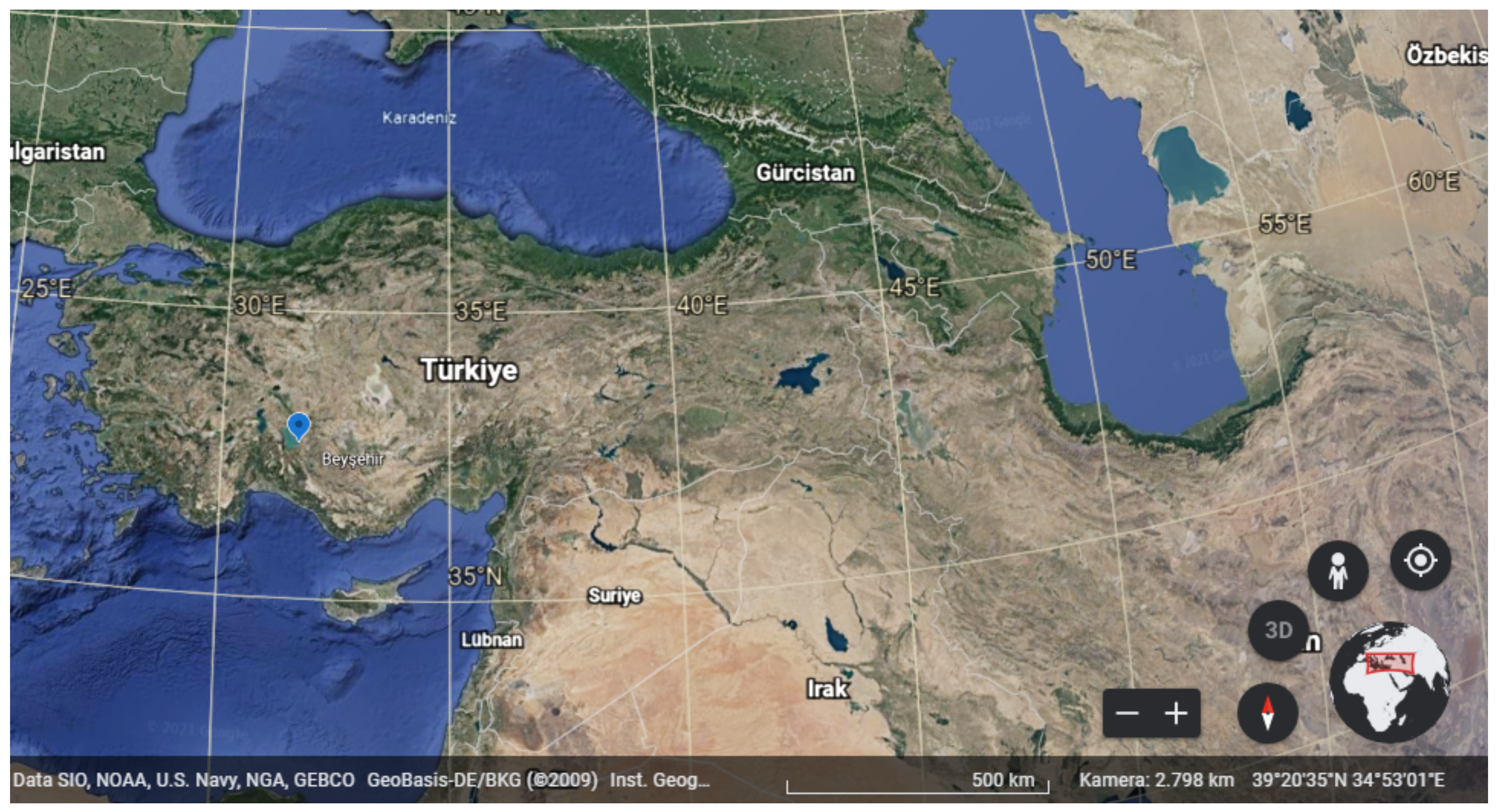
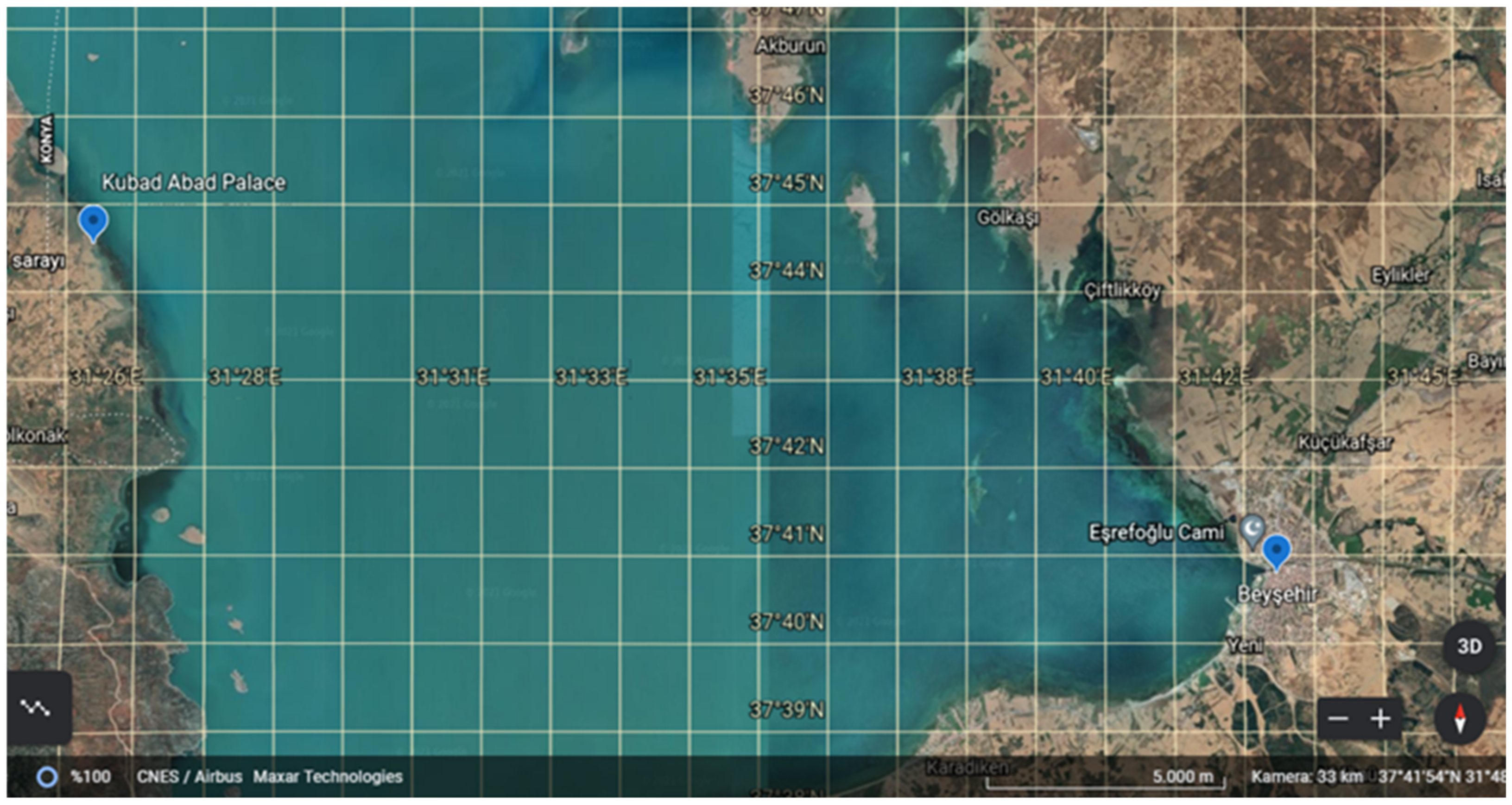
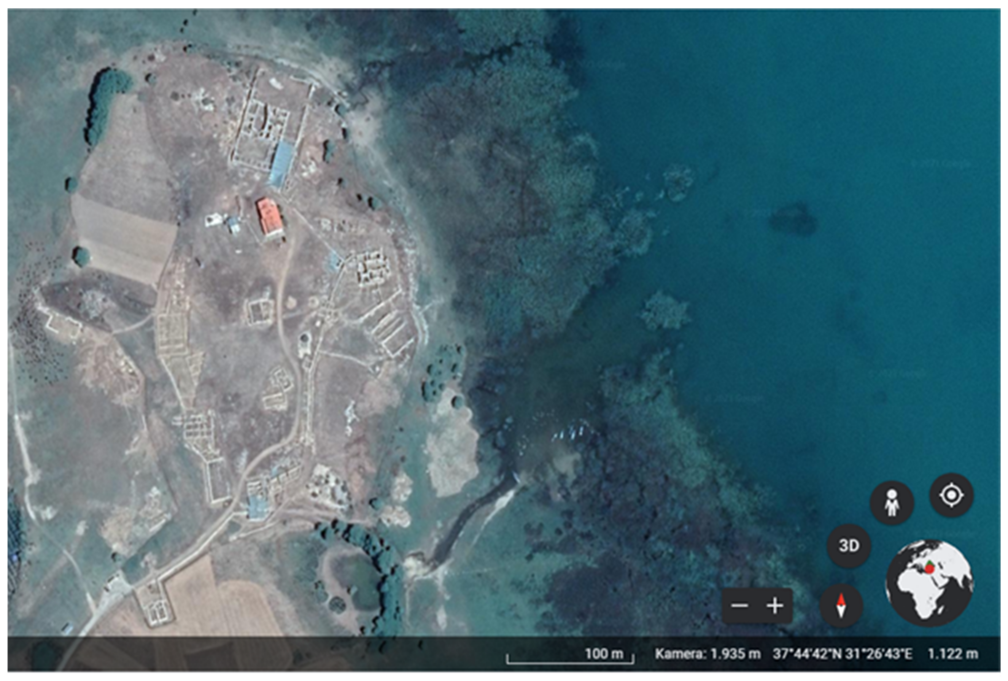
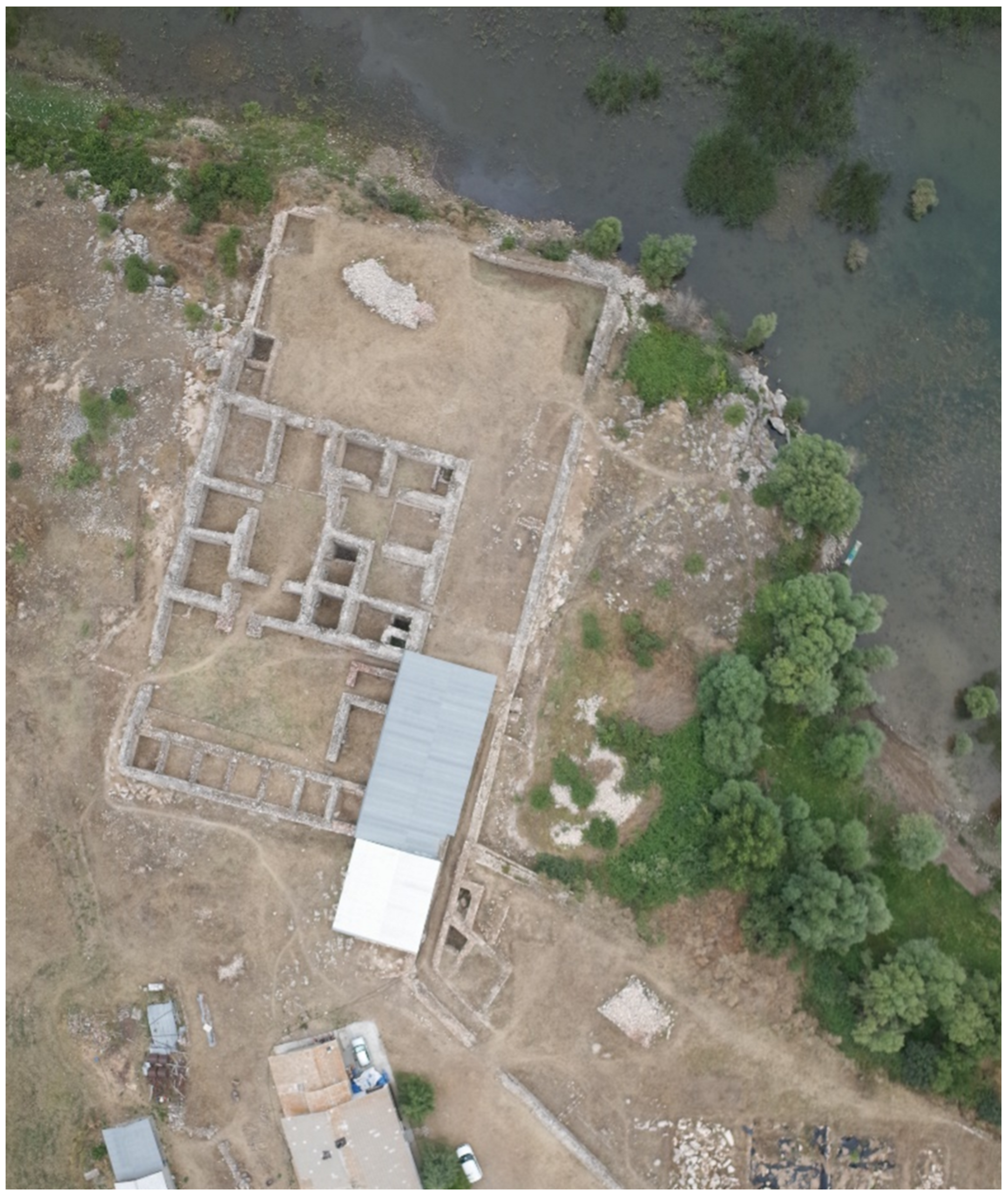
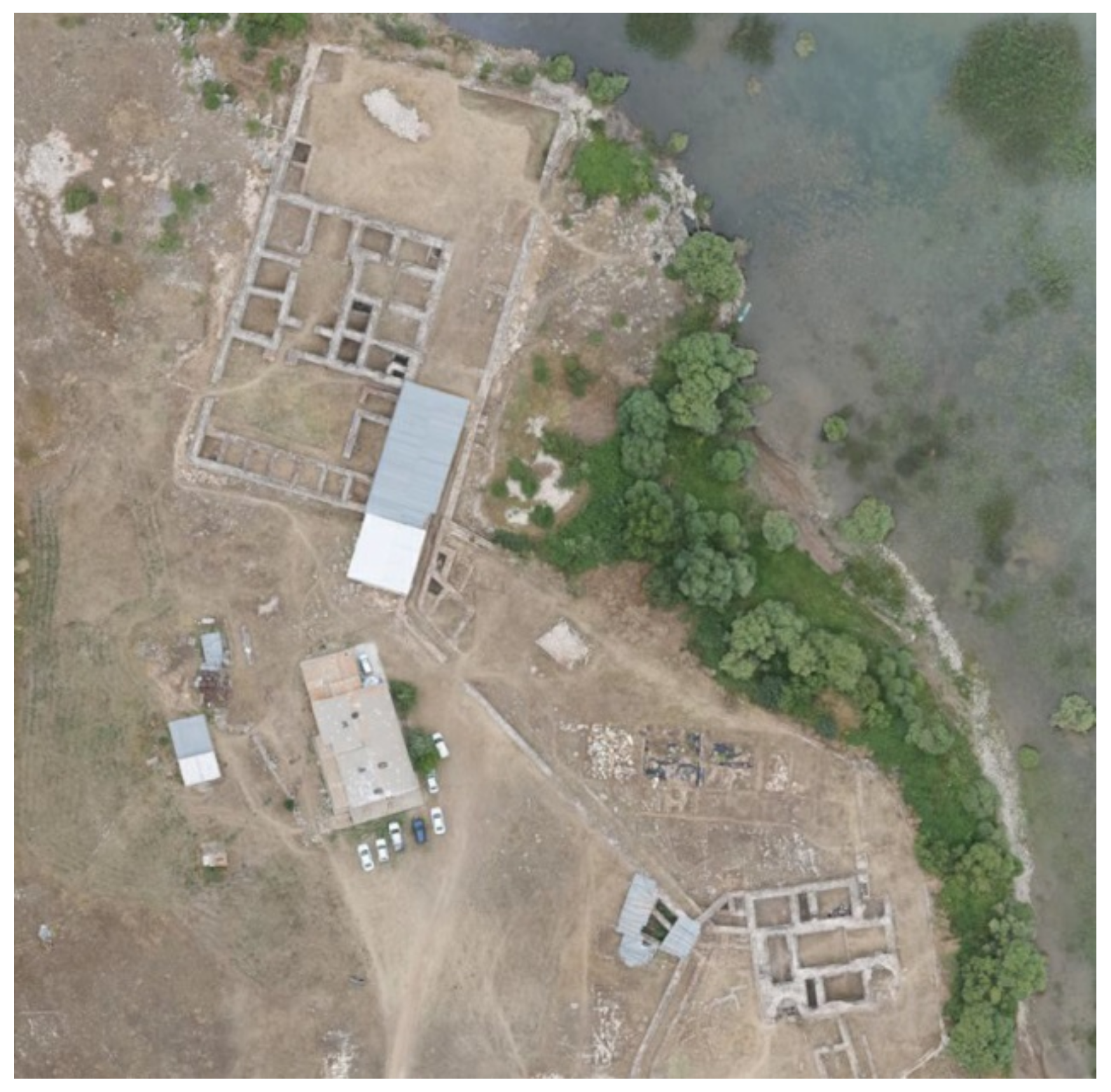
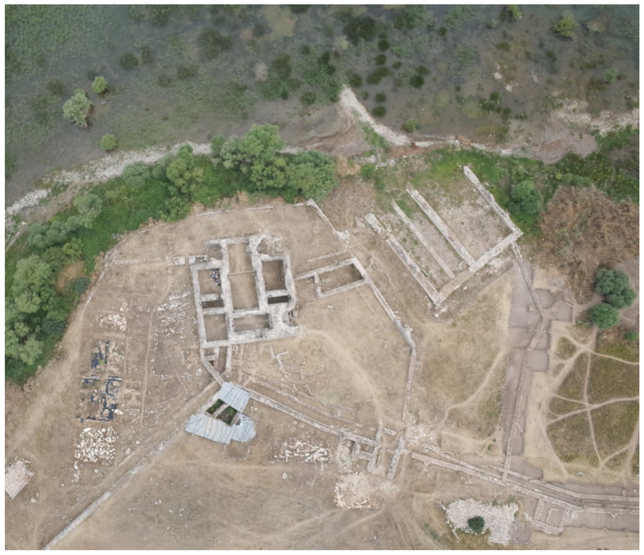
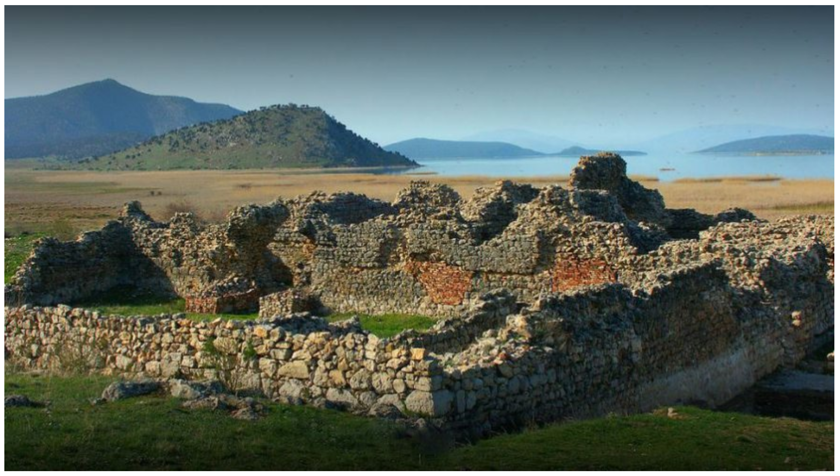
2. Kubad Abad Palace as Case Study
3. Materials and Methods
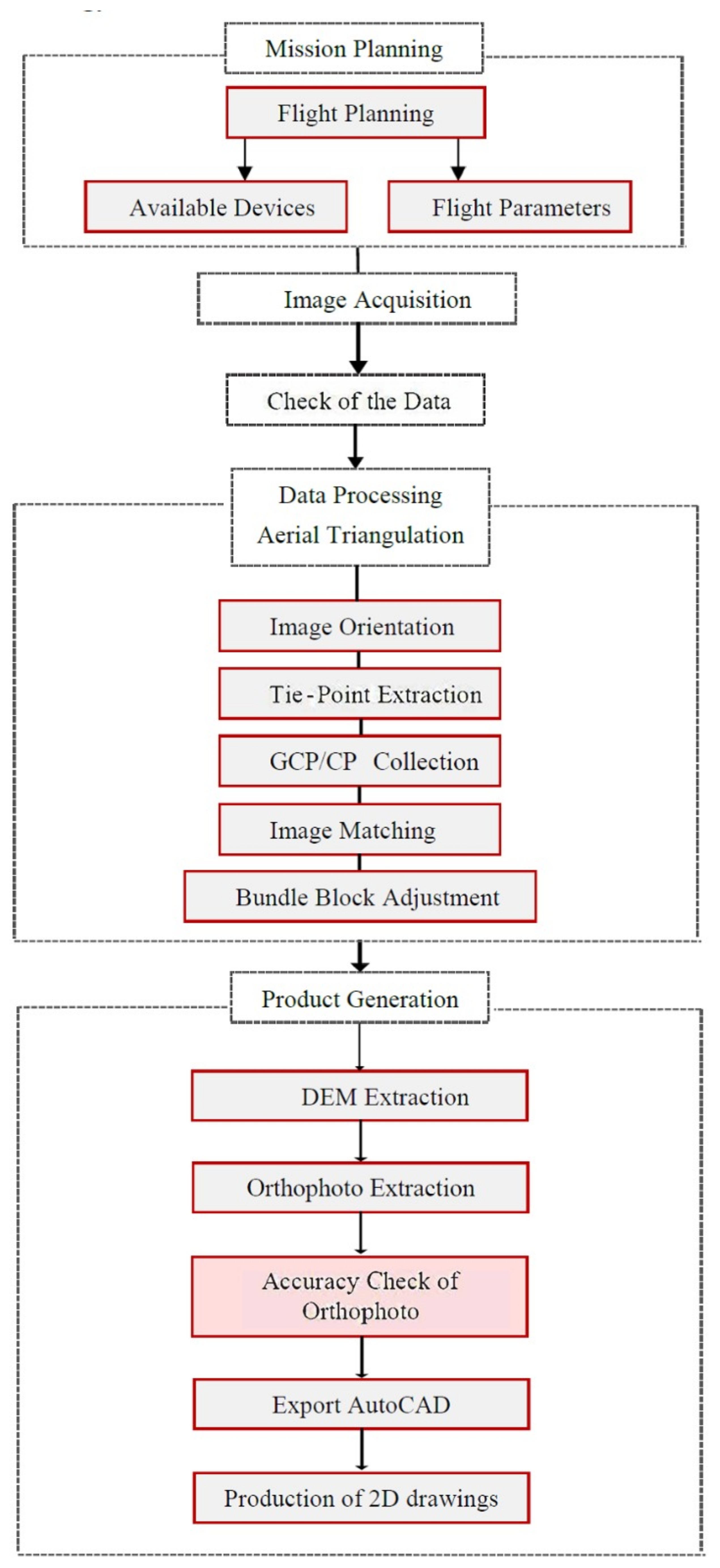
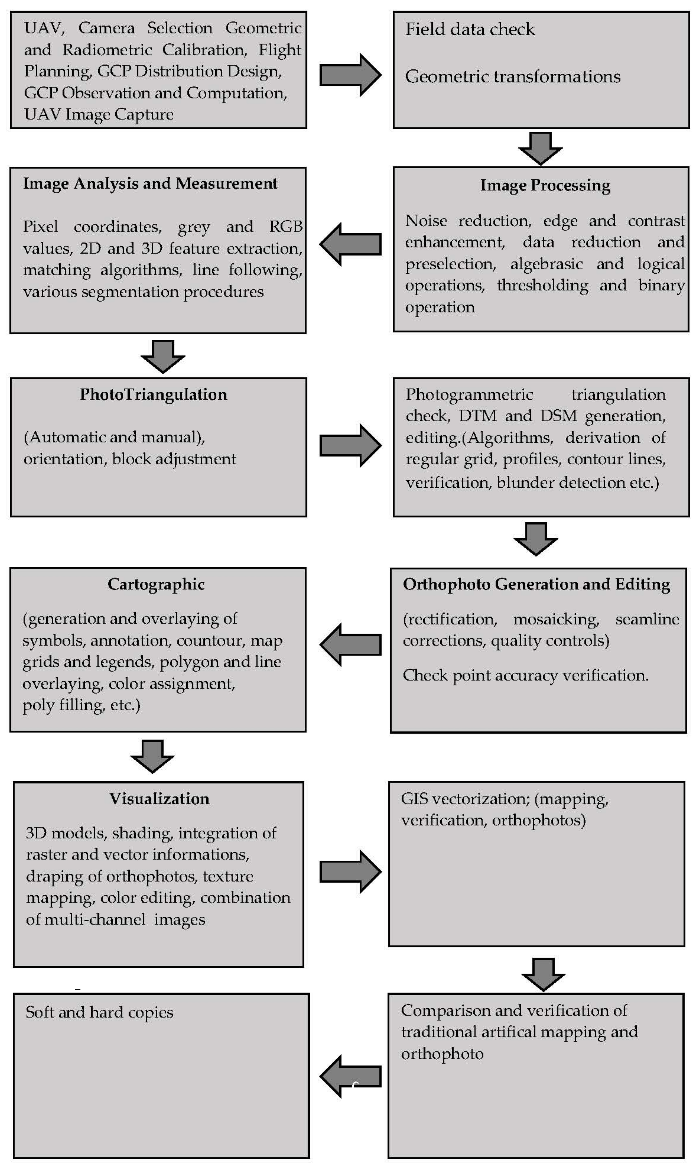
3.1. Methodology
3.1.1. Mission Planning
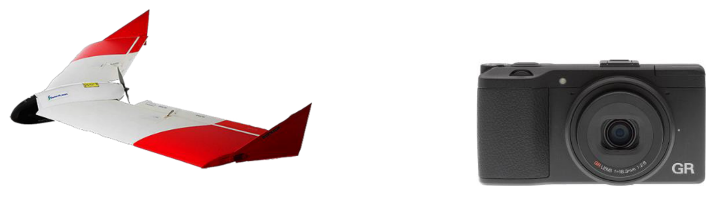
3.1.2. Image Acquisition
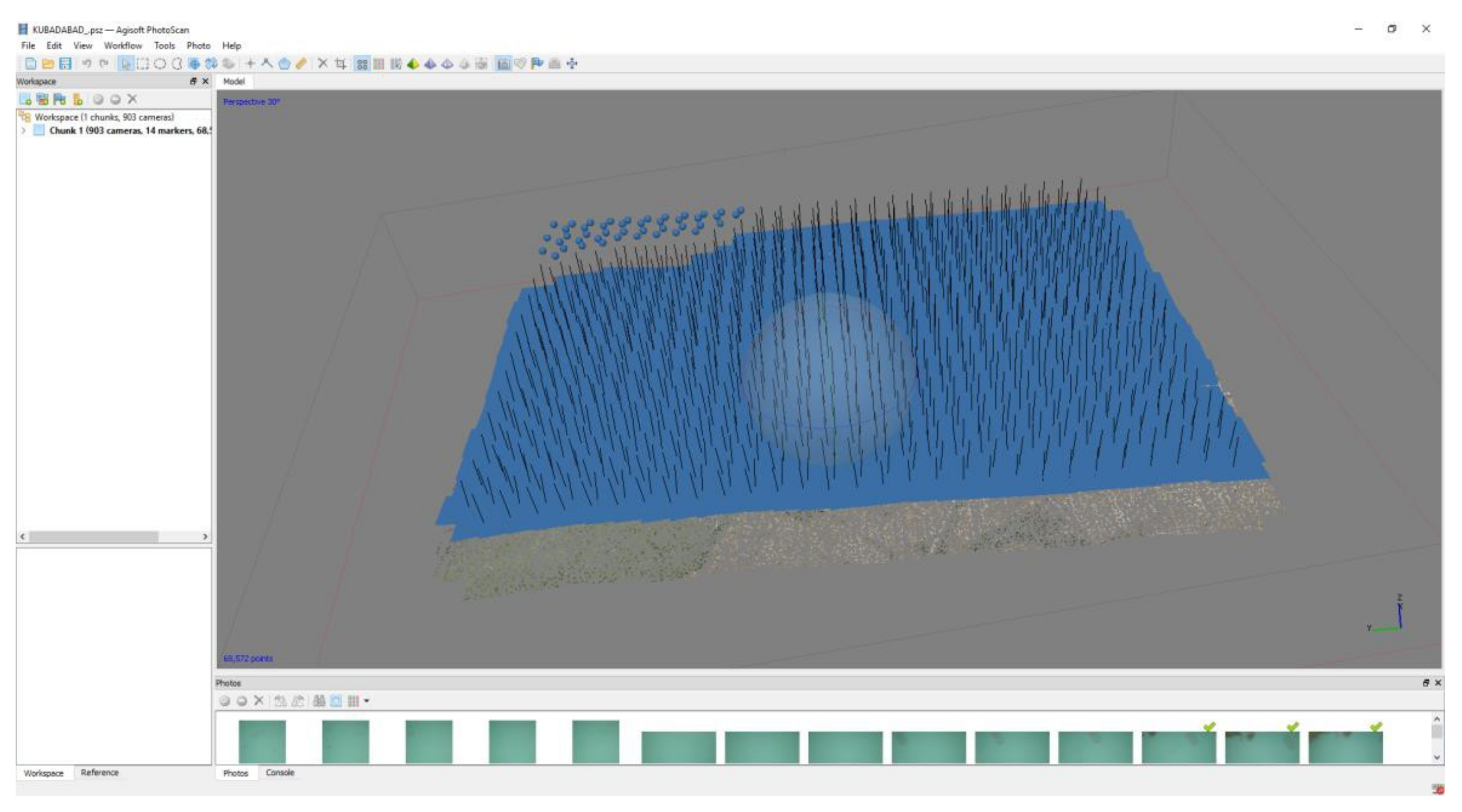
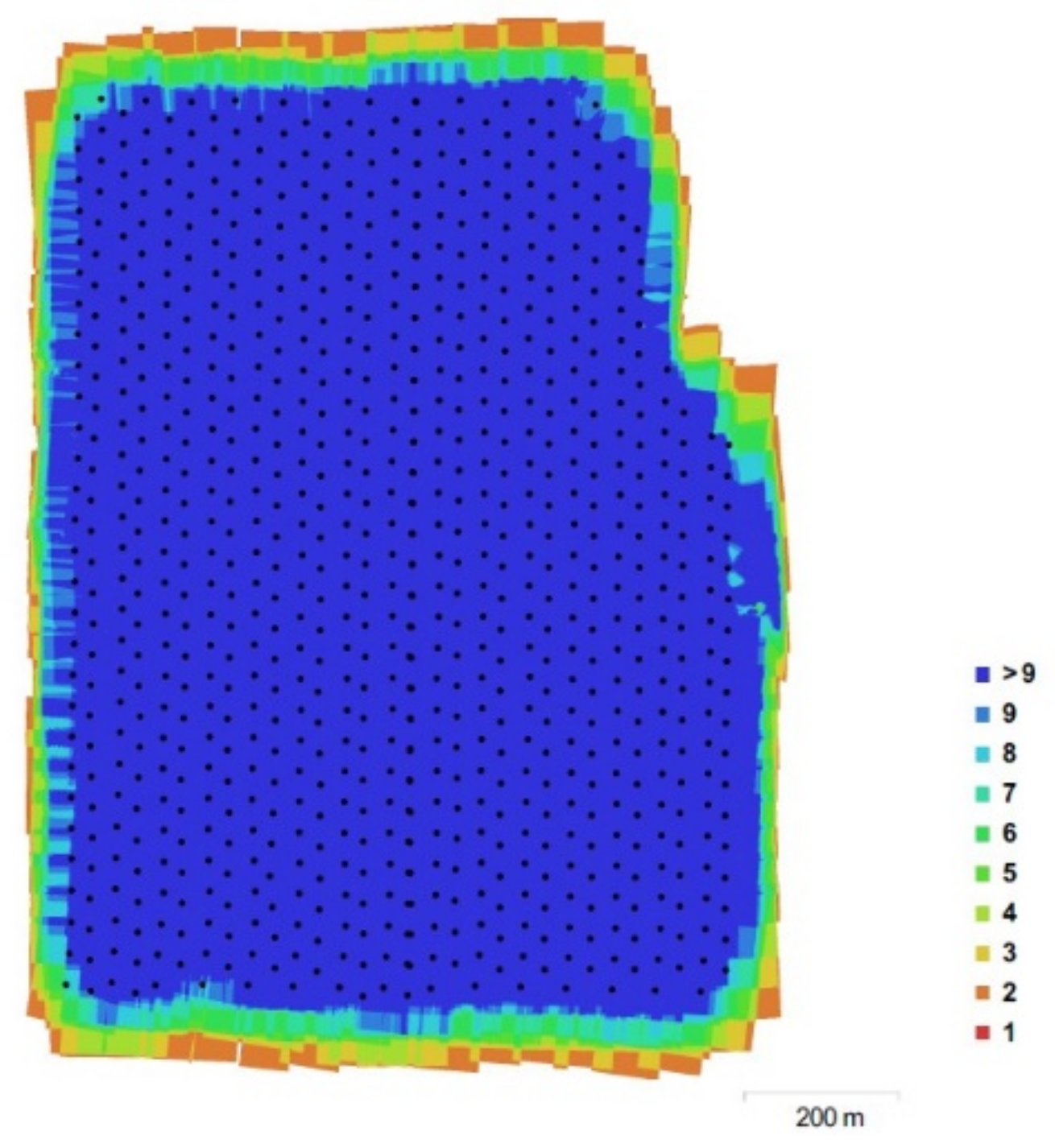
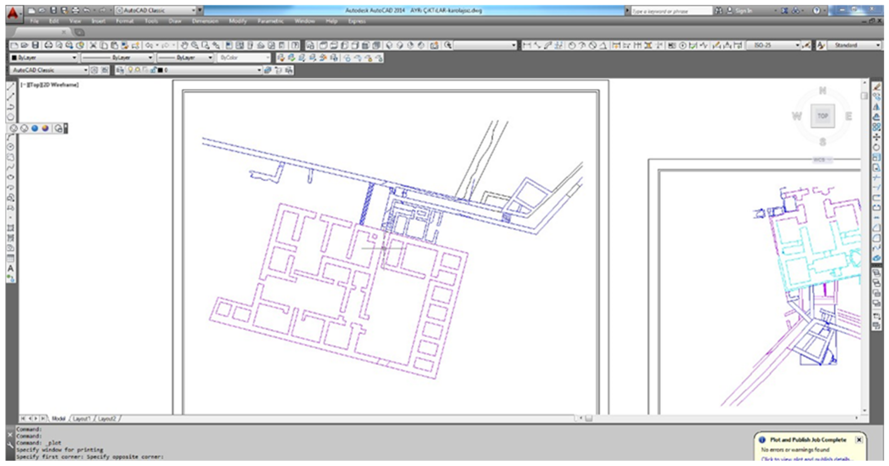
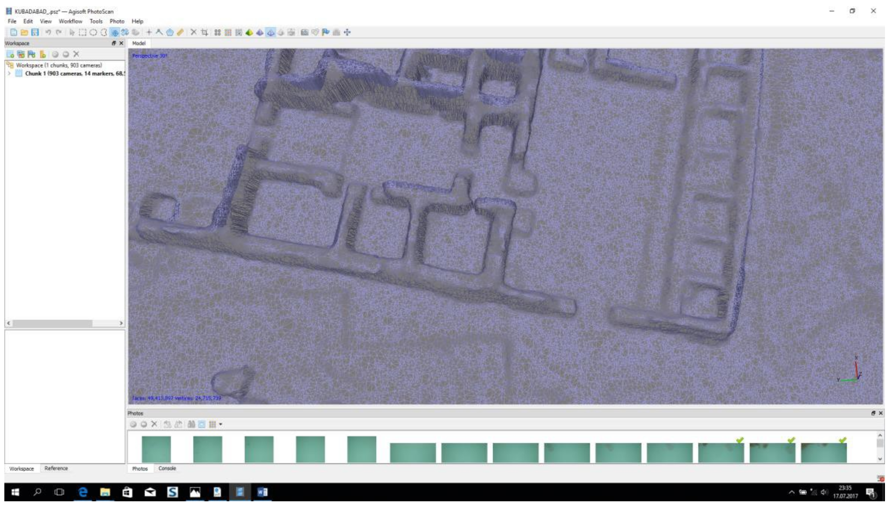
3.1.3. Data Processing (Aerial Triangulation)
4. Results
4.1. Specific Requirements
4.2. Horizontal and Vertical Accuracy Assessment
4.2.1. Horizontal Accuracy Assessment
4.2.2. Vertical Accuracy Assessment

| Vertical Accuracy Class | Absolute Accuracy | Relative Accuracy (Where Applicable) | ||||
|---|---|---|---|---|---|---|
| RMSEz Non-Vegetated (cm) | NVA at 95% Confidence Level (cm) | VVA at 95th Percentile (cm) | Within-Swath Hard Surface Repeatability (Max Diff) (cm) | Swath-to-Swath Non-Vegetated Terrain (RMSDz) (cm) | Swath-to-Swath Non-Vegetated Terrain (Max Diff) (cm) | |
| X-cm | ≤X | ≤1.96 x X | ≤3.00 x X | ≤0.60 x X | ≤0.80 x X | ≤1.60 x X |
4.3. A General Algorithm of the Case Study
5. Results
Author Contributions
Funding
Acknowledgments
Conflicts of Interest
References
- Eisenbeiss, H. A Mini Unmanned Aerial Vehicle [UAV]: System Overview and Image Acquisiton. In Proceedings of the International Workshop on Processing and Visualization Using High-Resolution Imagery, Pitsanulok, Thailand, 18–20 November 2004. [Google Scholar]
- Themistocleous, K. The use of UAVs to monitor archeological sites: The case study of Choirokoitia within the PROTHEGO project. In Proceedings of the Fifth International Conference on Remote Sensing and Geoinformation of the Environment [RSCy2017], Paphos, Cyprus, 20–23 March 2017; Volume 10444. [Google Scholar] [CrossRef]
- Bendea, H.; Chiabrandao, F.; Giulio Tonolo, F.; Marenchino, D. Mapping of archaeological areas using with a low-cost UAV the Augusta Bagiennorum test site. Presented at the XXI International CIPA Symposium, Athens, Greece, 1–6 October 2007. [Google Scholar]
- Remondino, F.; Barazzetti, L.; Nex, F.; Scaioni, M.; Sarazzi, D. UAV Photogrammetry for Mapping and 3D Modelling—Current Status and Future Perspectives. Presented at the ISPRS ICWG I/V-UAV-g [Unmanned Aerial Vehicle in Geomatics] Conference, Zurich, Switzerland, 14–16 September 2011. [Google Scholar]
- Patias, P.; Grussenmeyer, P.; Hanke, K. Applications in Cultural Heritage Documentation. Presented at the XXIth ISPRS Congress: Silk Road for Information from Imagery, Beijing, China, 3–11 July 2008. [Google Scholar]
- Cowley, D.C. Remote Sensing for Archaeological Heritage Management. Presented at the 11th EAC Heritage Management Symposium, Reykjavík, Iceland, 25–27 March 2010. [Google Scholar]
- Lo Brutto, M.; Borruso, A.; D’Argenio, A. UAV systems for photogrammetric data acquisition of archaeological sites. In Proceedings of the EUROMED 2012: Progress in Cultural Heritage Preservation, Limassol, Cyprus, 29 October–3 November 2012; pp. 7–13. [Google Scholar]
- Willis, M.D.; Koeing, C.W.; Black, S.L.; Castaneda, A.M. Archaeological 3D Mapping: The Structure from Motion Revolution. Index Tex. Archaeol. Open Access Gray Lit. Lone Star State 2016, 2016, 110. [Google Scholar]
- Eisenbeiß, H. UAV Photogrammetry. Ph.D. Thesis, ETH Zurich, Zürich, Switzerland, 2009. [Google Scholar]
- Mozas-Calvache, A.; Prez-Garca, J.; Cardenal-Escarcena, F.; Mata-Castro, E.; Delgado-Garca, J. Method for Photogrammetric Surveying of Archaeological Sites with Light Aerial Platforms. J. Archaeol. Sci. 2012, 39, 521–530. [Google Scholar] [CrossRef]
- Rinaudo, F.; Chiabrando, F.; Lingua, A.; Spanò, A. Archaeological Site Monitoring: UAV Photogrammetry can be an answer. Presented at the XXII ISPRS Congress, Melbourne, Australia, 25 August–1 September 2012. [Google Scholar]
- Anuar, A.; Khairul, N.T.; Wani, S.U.; Khairil, A.H.; NorHadija, D.; Mohd, H.; Shahrul, M.A. Digital Aerial Imagery of Unmanned Aerial Vehicle for Various Applications. Presented at the IEEE International Conference on Control System, Computing and Engineering, Penang, Malaysia, 29 November–1 December 2013. [Google Scholar]
- Sauerbier, M.; Eisenbeiss, H. UAV for the Documentation of Archaeological Excavations. Presented at the ISPRS 2010: Close Range Image Measurement Techniques, Newcastle upon Tyne, UK, 21–24 June 2010. [Google Scholar]
- Skarlatos, D.; Theodoridou, S.; Glabenas, D. Archaeological Surveys in Greece Using Radio Controlled Helicopter. Presented at the FIG Working Week 2004, Athens, Greece, 2–27 May 2004. [Google Scholar]
- Hendrickx, M.; Wouter Gheyle, W.; Bonne, J.; Bourgeois, J.; Wulf, A.; Goossens, R. The Use of Stereoscopic Images Taken from a Microdrone for the Documentation of heritage: An example from the Tuekta burial mounds in the Russian Altay. J. Archaeol. Sci. 2011, 38, 2968–2978. [Google Scholar] [CrossRef]
- Eisenbeiss, H.; Lambers, K.; Sauerbier, M. Photogrammetric Recording of the Archaeological Site of Pinchango Alto [Palpa, Peru] Using a mini Helicopter [UAV]. Presented at the CAA 2005: The World Is in Your Eyes: CAA 2005: Computer Applications and Quantitative Methods in Archaeology, Tomar, Portugal, 21–24 March 2005. [Google Scholar]
- Verhoeven, G.J.; Loenders, J.; Vermeulen, F.; Docter, R. Helikite aerial Photography or HAP—A versatile means of unmanned, radio controlled low altitude aerial archaeology. Archaeol. Prospect. 2009, 16, 125–138. [Google Scholar] [CrossRef]
- Haubeck, K.; Prinz, T. UAV-Based Low-Cost Stereo Camera System for Archaeological Surveys—Experiences from Doliche [Turkey]. Presented at the UAV-g2013, Rostock, Germany, 4–6 September 2013. [Google Scholar]
- Mesas-Carrascosa, J.F.; Rumbao, C.I.; Berrocal, B.A.J.; Porras, F.-G.A. Positional Quality Assessment of Orthophotos Obtained from Sensors Onboard multi-Rotor UAV Platforms. Sensors 2014, 14, 22394–22407. [Google Scholar] [CrossRef]
- Wemegah, D.T.; Amissah, B.M. Accuracy Checks in the Production of Orthophotos. J. Environ. Earth Sci. 2013, 3, 14–21. [Google Scholar]
- Liu, Y.; Zheng, X.; Ai, G.; Zhang, Y.; Zuo, Y. Generating a High-Precision true Digital Orthophoto Map Based on UAV Images. ISPRS Int. J. Geo-Inf. 2018, 7, 333. [Google Scholar] [CrossRef] [Green Version]
- Sai, S.S.; Tjahjadi, M.E.; Rokhmana, C.A. Geometric Accuracy Assessments of Orthophoto Production From UAV Aerial Images. In Proceedings of the 1st International Conference on Geodesy, Geomatics, and Land Administration 2019, Semarang, Indonesia, 24–25 July 2019; KnE Engineering: Semarang, Indonesia, 2019; pp. 333–344. [Google Scholar] [CrossRef]
- Wolf, R.P.; Dewit, A.B.; Wilkinson, E.B. Elements of Photogrammetry: With Applications in GIS, 3rd ed.; McGraw-Hill Companies Inc.: New York, NY, USA, 2000; pp. 217–225. [Google Scholar]
- United States Bureau of the Budget. United States National Map Accuracy Standards; Bureau of the Budget: Washington, DC, USA, 1947.
- Federal Geographic Data Committee [FGDC]. Revision of Geospatial Positioning Accuracy Standards, Part 3. In National Standard for Spatial Data Accuracy; fgdc-std-007.3-1998; FGDC Standard Projects. Available online: http://www.Fgdc.Gov/standards/projects/fgdc-standards-projects/accuracy/part3/nssda-revision-proposal (accessed on 26 December 2013).
- Standardization Agreements. In S. Standardization Agreement 2215: Evaluation of Land Maps, Aeronautical Charts and Digital Topographic Data; North Atlantic Treaty Organization: Bruxelles, Belgium, 2002.
- Greenfeld, J. Evaluating the Accuracy of Digital Orthophoto Quadrangles [DOQ] in the Context of Parcel-Based GIS. Photogramm. Eng. Remote Sens. 2001, 67, 199–206. [Google Scholar]
- Hashim, K.A.; Darwin, N.H.; Ahmad, A.; Samad, A.M. Assessment of low altitude aerial data for large scale urban environmental mapping. In Proceedings of the 2013 IEEE 9th International Colloquium on Signal Processing and Its Applications [CSPA], Kuala Lumpur, Malaysia, 8–10 March 2013; pp. 229–234. [Google Scholar]
- Tsarovski, S. Accuracy Evaluation and Quality Control of Digital Orthomap-Sheets. In Proceedings of the FIG Working Week 2015: From the Wisdom of the Ages to the Challenges of the Modern World, Sofia, Bulgaria, 17–21 May 2015. [Google Scholar]
- Julge, K.; Ellmann, A. Evaluating The Accuracy of Orthophotos and 3D Models from UAV Photogrammetry. In Geophysical Research Abstracts, Proceedings of the EGU General Assembly, Vienna, Austria, 12–17 April 2015; European Geosciences Union: Munich, Germany, 2015; Volume 17, p. EGU2015-655. [Google Scholar]
- Popescu, G.; Iordan, D.; Paunescu, V. The Resultant Positional Accuracy FOR THE Orthophotos obtained with Unmanned Aerial Vehicles [UAVs]. Sci. Agric. Agric. Sci. Procedia 2016, 10, 458–464. [Google Scholar] [CrossRef] [Green Version]
- Baehr, H.-P. Appropriate Pixel Size for Orthophotography. In Proceedings of the 17th ISPRS Congress, Washington, DC, USA, 2–14 August 1992; Volume 29, pp. 64–72. [Google Scholar]
- Kulur, S.; Yildiz, F.; Selcuk, O.; Yildiz, M.A. The Effect of Pixel Size on the Accuracy of Orthophoto Production. In Proceedings of the ISPRS Annals of the Photogrammetry, Remote Sensing and Spatial Information Sciences, XXIII ISPRS Congress, Prague, Czech Republic, 12–19 July 2016; Volume 3–4. [Google Scholar]
- Kapnias, D.; Milenov, P.; Kay, S. Guidelines for Best Practice and Quality Checking of Ortho Imagery; Joint Research Centre: Ispra, Italy, 2008. [Google Scholar]
- The American Society for Photogrammetry and Remote Sensing (ASPRS). Accuracy Standards for Digital Geospatial Data; ASPRS: Bethesda, MD, USA, 2013; Available online: www.asprs.org (accessed on 15 February 2018).
- Udin, W.S.; Ahmad, A. Assessment of Photogrammetric Mapping Accuracy Based on Variation Flying Altitude Using Unmanned Aerial Vehicle. IOP Conf. Ser. Earth Environ. Sci. 2014, 18, 012027. [Google Scholar] [CrossRef]
- Sisay, G.Z.; Besha, T.; Gessesse, B. Feature Orientation and Positional Accuracy Assessment of Digital Orthophoto and Line Map for Large Scale Mapping: The Case Stduy on Bahir Dar town, Ethiopia. In International Archives of the Photogrammetry, Remote Sensing and Spatial Information Sciences, Volume XLII-1/W1, Proceedings of the 2017 ISPRS Hannover Workshop: HRIGI 17–CMRT 17–ISA 17–EuroCOW 17, Hannover, Germany, 6–9 June 2017; International Society of Photogrammetry and Remote Sensing (ISPRS): Hannover, Germany, 2017. [Google Scholar]
- Arık, R. Kubad Abad Selçuklu Sarayı ve Çinileri; Türkiye İş Bankası Kültür Yayınları: Istanbul, Turkey, 2000. [Google Scholar]
- Daş, E. Kubadabad Palace. 2017. Available online: http://www.discoverislamicart.org (accessed on 15 February 2018).
- Available online: https://www.pusulahaber.com.tr/kubad-abad-sarayi-cinileriyle-goz-kamastiriyordu-7054yy.htm (accessed on 20 April 2021).
- Nex, F.; Remondino, F. UAV for 3D Mapping Applications: A Review. Appl. Geomat. 2014, 6, 1–15. [Google Scholar] [CrossRef]
- Xiang, H.; Tian, L. Development of a Low-Cost Agricultural Remote Sensing System Based on an Autonomous Unmanned Aerial Vehicle (UAV). Biosyst. Eng. 2011, 108, 174–190. [Google Scholar] [CrossRef]
- Chiang, W.-K.; Tsai, L.-M.; Naser, S.E.; Habib, A.; Chu, H.-C. A New Calibration Method Using Low Cost MEM IMUs to Verify the Performance of UAV-Borne MMS Payloads. Sensors 2015, 15, 6560–6585. [Google Scholar] [CrossRef] [PubMed] [Green Version]
- Rock, G.; Ries, J.B.; Udelhoven, T. Sensitivity Analysis of UAV-photogrammetry for creating digital elevation models (DEM). In International Archives of the Photogrammetry, Remote Sensing and Spatial Information Sciences, Vol. XXXVIII-1/C22 UAV-g 2011, Proceedings of the Conference on Unmanned Aerial Vehicle in Geomatics, Zurich, Switzerland, 14–16 September 2011; International Society of Photogrammetry and Remote Sensing (ISPRS): Hannover, Germany, 2011. [Google Scholar]
- Baltsavias, E.P.; Gruen, A.; Meister, M. DOW—A System Generation of Digital Orthophotos from Aerial and Spot Images. EARSel Adv. Remote Sens. 1992, 1, 105–112. [Google Scholar]


| Project Parameters | |
|---|---|
| Flight Height | 159 m |
| Ground resolution | 3.77 cm/px |
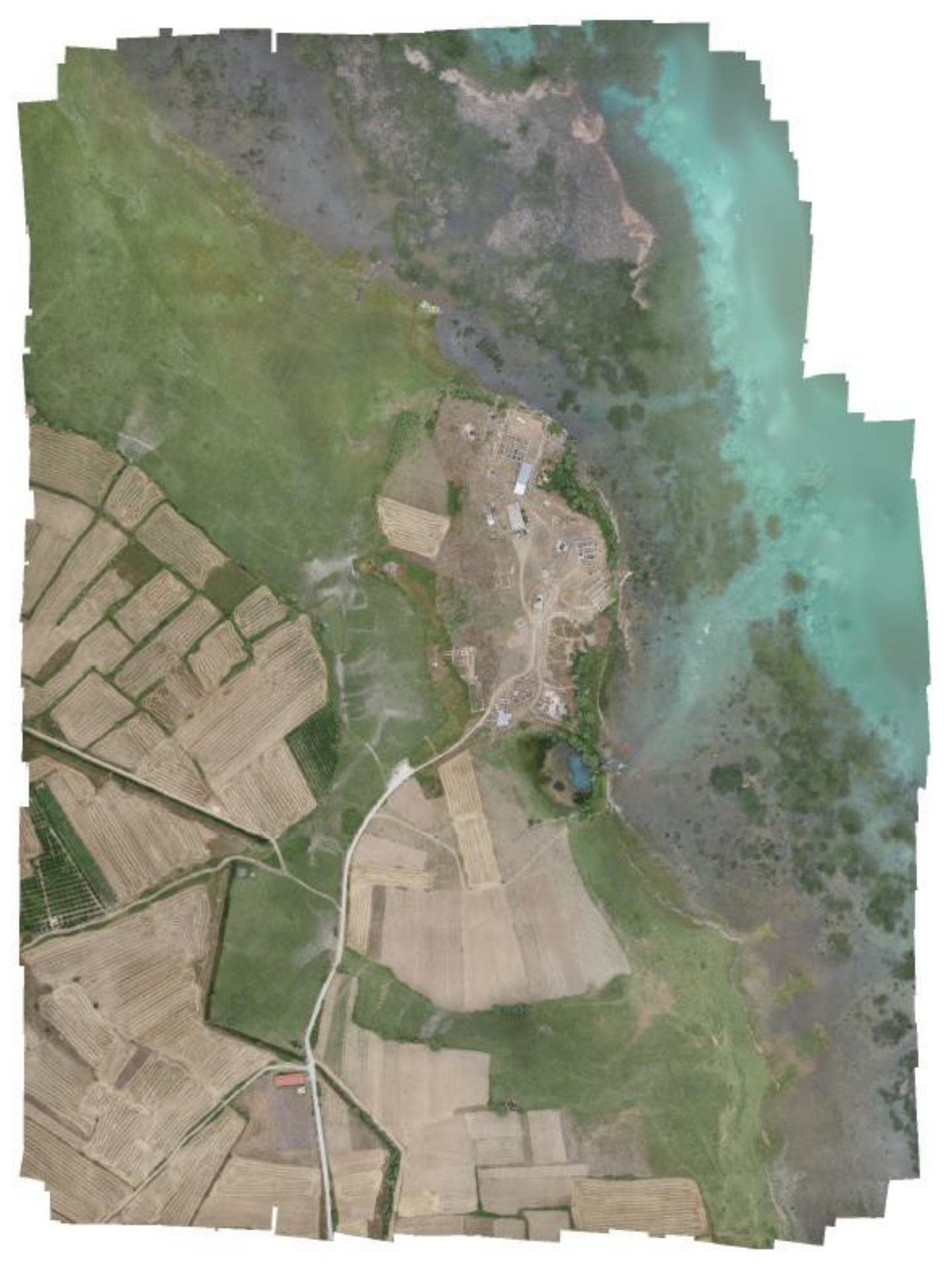
| Coverage area | 1.22 km2 |
| Sidelap | 60% |
| Overlap | 80% |
| Number of strips | 3 |
| Number of images | 903 |
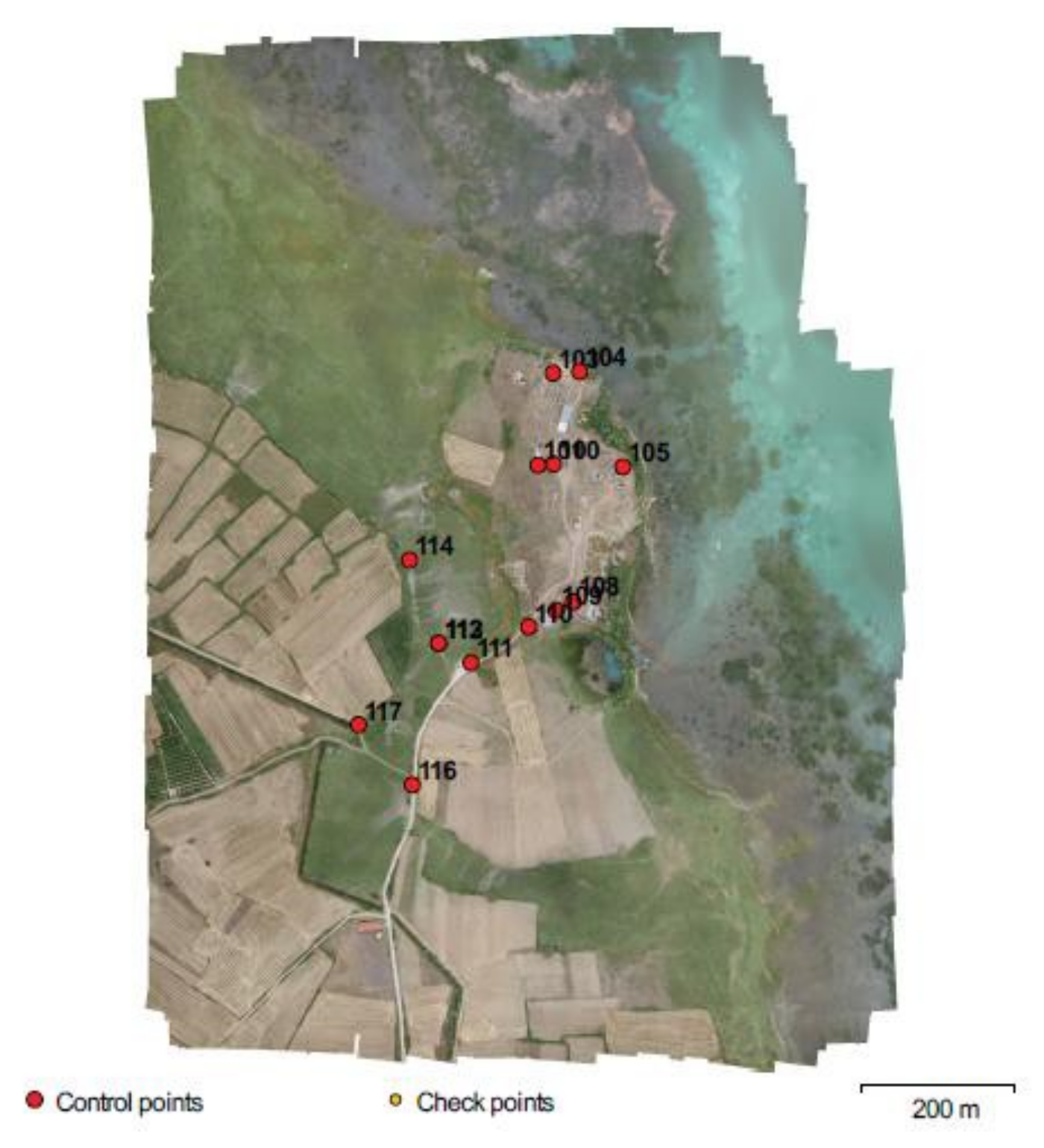
| Number of GCPs | 14 |
| Aligned cameras | 859 |
| Coordinate system | TUREF/TM 33 [EPSG:5255] |
| Dense point cloud points | 247,211,018 |
| Tie points | 68,572 |
| Projections | 611,032 |
| Reprojection error | 0.772 px |
| RMS reprojection error | 0.324 px |
| Faces | 49,413,897 |
| Vertices | 24,715,739 |
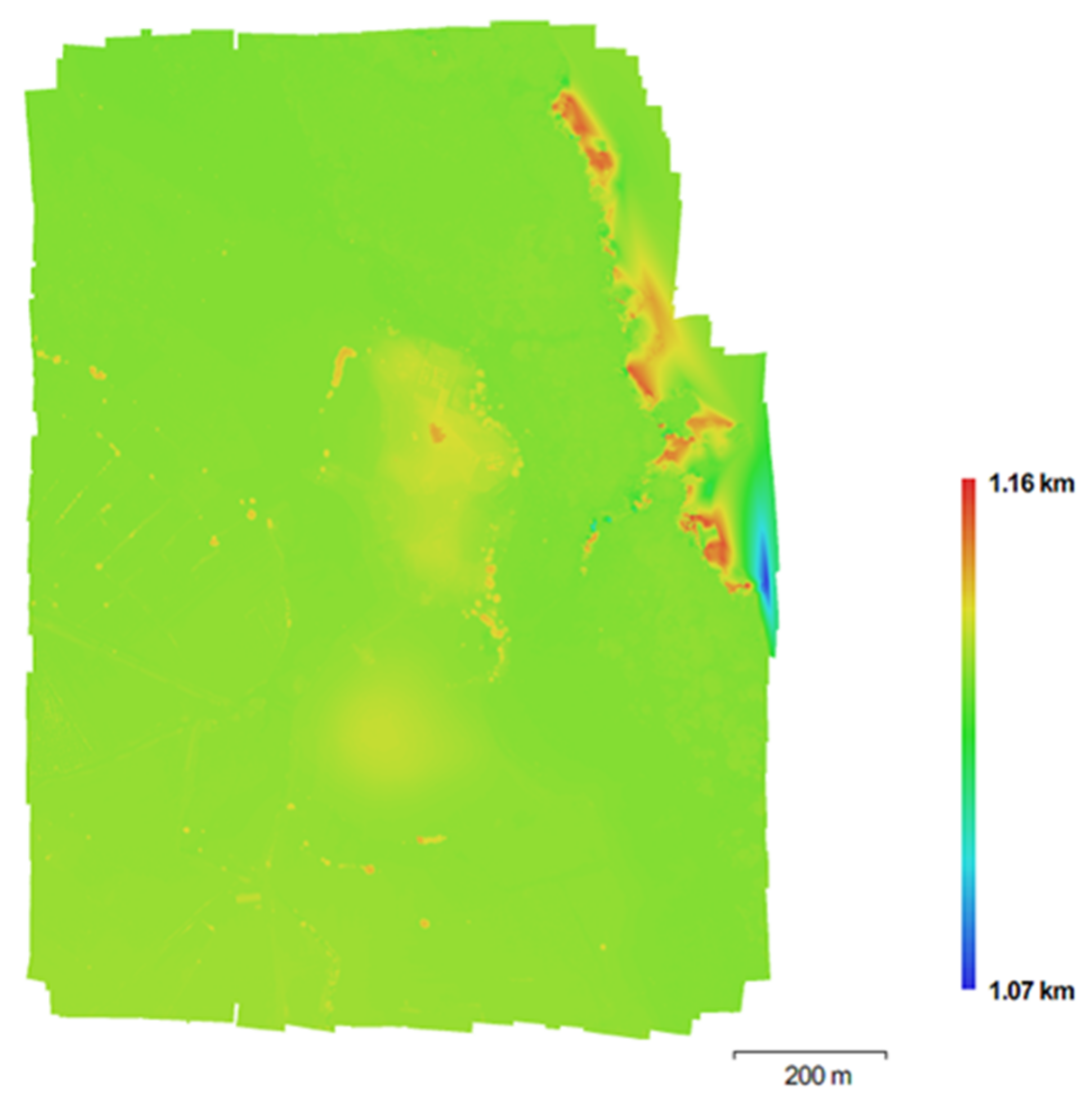
| DEM resolution | 7.55 cm/px |
| Orthomosaic size | 26,390 × 35,636 |
| Richor GR 18.3 mm Camera Calibration Parameters | |||
|---|---|---|---|
| Resolution | 4928 × 3264 | F | 3872.84 |
| Type | Frame | B1 | 0.441328 |
| Cx | −6.25894 | B2 | 2.37701 |
| Cy | 11.7735 | P1 | −0.000308219 |
| K1 | −0.0723221 | P2 | 2.6913 × 10⁻⁵ |
| K2 | 0.091206 | P3 | 0 |
| K3 | −0.0196215 | P4 | 0 |
| K4 | 0 | ||
| Count | X Error (cm) | Y Error (cm) | Z Error (cm) | XY Error (cm) | Total (cm) | Image (pix) |
|---|---|---|---|---|---|---|
| 14 | 4.06257 | 3.32436 | 3.28841 | 5.24937 | 6.19432 | 0.324 |
| Label | X Error (cm) | Y Error (cm) | Z Error (cm) | Total (cm) | Image (pix) |
|---|---|---|---|---|---|
| 100 | 6.11981 | 5.95244 | −1.88219 | 8.74221 | 0.269(23) |
| 101 | 4.45511 | −2.77318 | 3.11042 | 6.10027 | 0.310(24) |
| 103 | −4.27609 | −1.04231 | −2.03174 | 4.84761 | 0.266(18) |
| 104 | −3.38464 | −1.1302 | 1.253 | 3.78194 | 0.183(21) |
| 105 | 3.75177 | −5.17337 | −0.0764271 | 6.39103 | 0.121(22) |
| 108 | −0.994673 | 2.90823 | 6.45443 | 7.1489 | 0.346(25) |
| 109 | −8.0377 | 3.28298 | −6.07461 | 10.5964 | 0.556(24) |
| 110 | 2.599 | −2.00871 | −1.591775 | 3.65012 | 0.255(27) |
| 111 | 2.75833 | 1.93097 | 2.94591 | 4.47386 | 0.183(16) |
| 112 | −3.95106 | 2.24095 | −5.24227 | 6.93643 | 0.567(14) |
| 113 | 2.49822 | −1.3361 | 2.72138 | 3.92839 | 0.495(15) |
| 114 | −1.66697 | 4.1478 | −1.49671 | 4.71415 | 0.051(4) |
| 116 | −3.39311 | −0.623031 | −1.28622 | 3.68181 | 0.177(17) |
| 117 | 3.72089 | −5.57416 | 1.97885 | 6.988 | 0.118(16) |
| Total | 4.06257 | 3.32436 | 3.28841 | 6.19432 | 0.324 |
| Project Area (Square Kilometers) | Horizontal Accuracy Testing of Orthoimagery and Planimetrics | Vertical and Horizontal Accuracy Testing of Elevation Data Sets | ||
|---|---|---|---|---|
| Total Number of Static 2D/3D Check Points (Clearly Defined Points) | Number of Static 3D Check Points in NVA | Number of Static 3D Check Points in VVA | Total Number of Static 3D Check Points | |
| ≤500 | 20 | 20 | 5 | 25 |
| 501–750 | 25 | 20 | 10 | 30 |
| 751–1000 | 30 | 25 | 15 | 40 |
| 1001–1250 | 35 | 30 | 20 | 50 |
| 1251–1500 | 40 | 35 | 25 | 60 |
| 1501–1750 | 45 | 40 | 30 | 70 |
| 1751–2000 | 50 | 45 | 35 | 80 |
| 2001–2250 | 55 | 50 | 40 | 90 |
| 2251–2500 | 60 | 55 | 45 | 100 |
| Horizontal Accuracy Class | RMSEx and RMSEy (cm) | RMSEr (cm) | Horizontal Accuracy at 95% Confidence Level (cm) | Orthoimagery Mosaic Seamline Mismatch (cm) |
|---|---|---|---|---|
| X-cm | ≤X | ≤1.41 x X | ≤2.45 x X | ≤2 xX |
| Horizontal Accuracy Class RMSEx and RMSEy (cm) | RMSEr (cm) | Orthoimage Mosaic Seamline Maximum Mismatch (cm) | Horizontal Accuracy at the 95% Confidence Level (cm) |
|---|---|---|---|
| 0.63 | 0.9 | 1.3 | 1.5 |
| 1.25 | 1.8 | 2.5 | 3.1 |
| 2.50 | 3.5 | 5.0 | 6.1 |
| 5.00 | 7.1 | 10.0 | 12.2 |
| 7.50 | 10.6 | 15.0 | 18.4 |
| 10.00 | 14.1 | 20.0 | 24.5 |
| 12.50 | 17.7 | 25.0 | 30.6 |
| 15.00 | 21.2 | 30.0 | 36.7 |
| 17.50 | 24.7 | 35.0 | 42.8 |
| 20.00 | 28.3 | 40.0 | 49.0 |
| 22.50 | 31.8 | 45.0 | 55.1 |
| 25.00 | 35.4 | 50.0 | 61.2 |
| 27.50 | 38.9 | 55.0 | 67.3 |
| 30.00 | 42.4 | 60.0 | 73.4 |
| 45.00 | 63.6 | 90.0 | 110.1 |
| 60.00 | 84.9 | 120.0 | 146.9 |
| 75.00 | 106.1 | 150.0 | 183.6 |
| 100.00 | 141.4 | 200.0 | 244.8 |
| 150.00 | 212.1 | 300.0 | 367.2 |
| 200.00 | 282.8 | 400.0 | 489.5 |
| 250.00 | 353.6 | 500.0 | 611.9 |
| 300.00 | 424.3 | 600.0 | 734.3 |
| 500.00 | 707.1 | 1000.0 | 1223.9 |
| 1000.00 | 1414.2 | 2000.0 | 2447.7 |
| ASPRS 2014 | Equivalent to Map Scale in | ||||
|---|---|---|---|---|---|
| Horizontal Accuracy Class RMSEx and RMSEy (cm) | RMSEr (cm) | Horizontal Accuracy at the 95% Confidence Level (cm) | Approximate GSD of Source Imagery (cm) | ASPRS1990 Class 1 | ASPRS1990 Class 2 |
| 0.63 | 0.9 | 1.5 | 0.31 to 0.63 | 1:25 | 1:12.5 |
| 1.25 | 1.8 | 3.1 | 0.63 to 1.25 | 1:50 | 1:25 |
| 2.5 | 3.5 | 6.1 | 1.25 to 2.5 | 1:100 | 1:50 |
| 5.0 | 7.1 | 12.2 | 2.5 to 5.0 | 1:200 | 1:100 |
| 7.5 | 10.6 | 18.4 | 3.8 to 7.5 | 1:300 | 1:150 |
| 10.0 | 14.1 | 24.5 | 5.0 to 10.0 | 1:400 | 1:200 |
| 12.5 | 17.7 | 30.6 | 6.3 to12.5 | 1:500 | 1:250 |
| 15.0 | 21.2 | 36.7 | 7.5 to 15.0 | 1:600 | 1:300 |
| 17.5 | 24.7 | 42.8 | 8.8 to 17.5 | 1:700 | 1:350 |
| 20.0 | 28.3 | 49.0 | 10.0 to 20.0 | 1:800 | 1:400 |
| 22.5 | 31.8 | 55.1 | 11.3 to 22.5 | 1:900 | 1:450 |
| 25.0 | 35.4 | 61.2 | 12.5 to 25.0 | 1:1000 | 1:500 |
| 27.5 | 38.9 | 67.3 | 13.8 to 27.5 | 1:1100 | 1:550 |
| 30.0 | 42.4 | 73.4 | 15.0 to 30.0 | 1:1200 | 1:600 |
| Vertical Accuracy Class | Absolute Accuracy | Relative Accuracy (Where Applicable) | ||||
|---|---|---|---|---|---|---|
| RMSEz Non-Vegetated (cm) | NVA at 95% Confidence Level (cm) | VVA at 95th Percentile (cm) | Within-Swath Hard Surface Repeatability (Max Diff) (cm) | Swath-to-Swath Non-Veg Terrain (RMSDz) (cm) | Swath-to-Swath Non-Veg Terrain (Max Diff) (cm) | |
| 1 m | 1.0 | 2.0 | 3 | 0.6 | 0.8 | 1.6 |
| 2.5-cm | 2.5 | 4.9 | 7.5 | 1.5 | 2 | 4 |
| 5-cm | 5.0 | 9.8 | 15 | 3 | 4 | 8 |
| 10-cm | 10.0 | 19.6 | 30 | 6 | 8 | 16 |
| 15-cm | 15.0 | 29.4 | 45 | 9 | 12 | 24 |
| 20-cm | 20.0 | 39.2 | 60 | 12 | 16 | 32 |
| 33.3-cm | 33.3 | 65.3 | 100 | 20 | 26.7 | 53.3 |
| 66.7-cm | 66.7 | 130.7 | 200 | 40 | 53.3 | 106.7 |
| 100-cm | 100.0 | 196.0 | 300 | 60 | 80 | 160 |
| 333.3-cm | 333.3. | 653.3 | 1000 | 200 | 266.7 | 533.3 |
Publisher’s Note: MDPI stays neutral with regard to jurisdictional claims in published maps and institutional affiliations. |
© 2021 by the authors. Licensee MDPI, Basel, Switzerland. This article is an open access article distributed under the terms and conditions of the Creative Commons Attribution (CC BY) license (https://creativecommons.org/licenses/by/4.0/).
Share and Cite
Korumaz, S.A.G.; Yıldız, F. Positional Accuracy Assessment of Digital Orthophoto Based on UAV Images: An Experience on an Archaeological Area. Heritage 2021, 4, 1304-1327. https://doi.org/10.3390/heritage4030071
Korumaz SAG, Yıldız F. Positional Accuracy Assessment of Digital Orthophoto Based on UAV Images: An Experience on an Archaeological Area. Heritage. 2021; 4(3):1304-1327. https://doi.org/10.3390/heritage4030071
Chicago/Turabian StyleKorumaz, Saadet Armağan Güleç, and Ferruh Yıldız. 2021. "Positional Accuracy Assessment of Digital Orthophoto Based on UAV Images: An Experience on an Archaeological Area" Heritage 4, no. 3: 1304-1327. https://doi.org/10.3390/heritage4030071
APA StyleKorumaz, S. A. G., & Yıldız, F. (2021). Positional Accuracy Assessment of Digital Orthophoto Based on UAV Images: An Experience on an Archaeological Area. Heritage, 4(3), 1304-1327. https://doi.org/10.3390/heritage4030071