Solid Model Generation for Digitized Organic Bodies via T-Splines


Department of Architecture, Built Environment and Construction Engineering (ABC), Politecnico di Milano, Via Ponzio 31, 20133 Milan, Italy
Heritage 2020, 3(3), 606-636; https://doi.org/10.3390/heritage3030035
Submission received: 9 June 2020
/
Revised: 25 June 2020
/
Accepted: 28 June 2020
/
Published: 30 June 2020
Abstract
:This paper presents a workflow for B-rep solid model generation of organic objects using T-splines constructed with quad-meshes. The aim is the creation of geometrically and topologically consistent B-rep solid models of heritage objects featuring organic shapes, which can be used in numerical simulation based on meshless finite element analysis. Point clouds and closed triangular meshes are converted into B-rep solids with a multi-step procedure based on the preliminary extraction of quadrilateral meshes, which are used to produce T-splines. Evaluation of metric quality is carried out to quantify the difference between the final solid and input datasets. A coarse-to-fine approach can also be exploited by varying the quad-mesh resolution to preserve the level of details captured during the digitization process. Finally, meshless finite element analysis can be run with the produced solid bodies. Results for both simulated and real heritage objects are illustrated and discussed.
1. Introduction
1.1. Preliminary Concepts on Digitization, Solid Modeling Techniques and Meshless FEA
Digitization of heritage objects is a field of research that involves a wide community of operators such as archeologists, architects, engineers, restorers, computer science specialists, surveyors, conservators, among others. Several digitization projects are reported in technical literature and deal with different techniques (the reader is referred to References [1,2,3,4,5,6,7,8,9,10,11,12] for a few examples).
The commercial market offers several products able to reconstruct the surface of an object by point clouds and/or meshes [13]. The most common solutions are laser scanners, structured light systems and digital photogrammetry [14]. In recent years, the rapid development of algorithms and sensors as well as the improved level of automation has made available powerful digitalization tools not only for specialists in the field of surveying and 3D modeling. Nowadays, several specialists operating in different fields can use such digital tools and generate 3D digital reconstructions of different categories of heritage objects like historic buildings, archeological sites, paintings, statues, artifacts, bas-reliefs and so forth. The use of digital images captured with consumer-grade digital cameras and then processed in software packages able to extract a 3D model has widened the community of operators interested in accurate digital reconstructions [15]. A comprehensive review of digitization methods is illustrated and discussed in References [16,17,18,19].
Although modern digitalization tools can capture a huge number of measurements in a relatively short time, the produced output is not always the final deliverable of the project. For instance, images captured with a drone can be automatically processed to generate orthophotos and digital terrain models of archeological areas but the generation of CAD (Computer-aided design) drawings requires extensive manual tracing. In the case of historical buildings surveyed with a laser scanner, the production of accurate 3D models or BIM (Building Information Modeling) still requires manual modeling in specific software [20]. The creation of digital reconstructions of small artifacts often requires manual editing in reverse engineering software [21].
Operators involved in heritage recording known that extra (often manual) work is usually required notwithstanding specific software can assist the operator with automatic and semi-automatic procedures. Manual work is also necessary for the need for human interpretation, which can be a real challenge for heritage objects. Although recent developments and research work in the field of semantic segmentation and deep learning are very promising [22,23], some operations still need expert (human) operators. An example is the accurate separation of constructive elements (such as stairs, walls, windows, doors, …) in 3D modeling of buildings surveyed with point clouds. Similarly, recognizing the different stratigraphic layers in archeology needs human interpretation. Probably, heritage objects will remain a complicated and stimulating challenge for their intrinsic complexity.
This paper describes a workflow able to generate a 3D solid model based on B-rep (boundary representation [24,25]) for objects digitally reconstructed with a point cloud or triangular mesh. The idea is trying to simplify and automate the production of B-rep solid models of complex shapes to be used in meshless finite element analysis, for which manual modeling would require extensive work. The workflow is synthetically illustrated in Figure 1, where a triangular mesh has been generated using Reality Capture and a set of 297 images.
The object is a pre-Islamic basket-shaped pottery container with a large arched handle. It is on display in the Mleiha Archaeological Center and it was captured and made available by Global Digital Heritage (GDH), which is an organization dedicated to documenting, monitoring and preserving global cultural and natural heritage. As mentioned, the conversion of the initial mesh (A) into a solid model would enable numerical simulation, among which finite element analysis (FEA). The proposed approach is based on the conversion of the tri-mesh into T-splines [26] based on quad-meshes [27] (B), which are then automatically turned into a B-rep solid (C). Finally, meshless finite element analysis (FEA) [28] is used for the numerical simulation (D).
The method has a very high level of automation notwithstanding some manual corrections could be necessary to fix local geometric and topological mistakes. It provides statistics to evaluate the difference between the original point cloud (or the initial tri-mesh) and the final solid model. Such quantity is used as an indicator of the achieved metric quality. The expected result is a detailed, consistent and complete B-rep solid model of irregular objects without excessive simplification. As the 3D solid model defines a closed volume and combines geometrical and topological information (i.e., an unambiguous model), it can be used for meshless FEA.
1.2. Some Considerations on the Geometry: Organic vs Geometric Shapes
One of the advantages of the proposed method is the automation level in the generation of a 3D solid model (not only a surface) for complex and irregular objects. Nowadays, the generation of mesh surfaces that accurately represent objects is a relatively standard procedure. However, the production of solid models is still a complicated task in the case of objects which cannot be modeled with basic primitives and/or NURBS (Non-uniform rational basis spline) functions. The paper will, therefore, focus on a procedure for 3D solid modeling in the case of free-form objects scanned via point clouds or meshes. This also permits the reuse of existing models. The case of organic shapes [29] will be considered, that is those shapes that are irregular, imperfect, different from one another, with curved structures and no hard angles. Several heritage objects belong to this category like statues of human or animal figures, fossils, stalactites and stalagmites (Figure 2).
The term “organic” used in this manuscript defines those shapes that are the opposite of geometric shapes (also called nonorganic, inorganic or hard-surface models), which are shapes with clear corners and edges, that is, the typical case of man-made objects whereas organic shapes are mainly related to natural objects (fruit, vegetation, animals, etc.). However, the distinction used in this paper is purely geometric and comes from the 3D modeling sector, as illustrated in Reference [29]. Confusion with other possible definitions related to the term organic (such as in natural science, chemistry and archeology) must be avoided.
An overall (geometric) criterium for separating organic and geometric shapes is not available. Figure 3 shows some (man-made) architectures with inorganic shape (A, B), which could be modeled using surfaces connected with sharp edges. The amethyst has also a clear geometric shape (C), notwithstanding it comes from the natural world.
As mentioned, the paper will concentrate on the solid modeling of both natural and man-made organic objects, showing a procedure to generate B-rep solids with a multi-step procedure. Solid modeling [30] is a field of research based on mathematics and computational geometry, with a strong relationship to computer graphics. Objects can be pure geometric, organic shapes or a combination of both categories. Solid modeling from point clouds and meshes is a very important topic in reverse engineering applications, especially those related the mechanical and manufacturing engineering. The commercial market offers software for the creation of assemblies in different applications like the aerospace, automotive, machinery, electronics, medicine and product design industries. Such software packages provide advanced tools for numerical simulation including static and dynamics structural analysis, natural mode shapes and frequencies determination, thermal behavior, impact simulation, among others. The market also offers combined CAD (Computer-aided design), CAE (Computer-aided engineering) and CAM (Computer-aided manufacturing) solutions such as Solidworks, Solid Edge, Fusion 360, Inventor, CATIA, Creo and Onshape.
It is the author’s opinion that the direct use of the solution developed for industrial/mechanical applications can be exploited for digital documentation of cultural heritage but some important aspects must be carefully taken into consideration to understand (and accept) some limitations. For instance, reverse engineering of industrial components [31] can deal with complex surfaces such as characters for the entertainment industry, some cars like the Volkswagen Beetle or small objects like some jewels. A heritage objects can be not only complex but also unique of its kind. Precise and detailed reconstructions should consider the imperfections and irregularities which characterize each object An excessive simplification during the (solid) modeling process could lose the “anomalies” that distinguish that object.
Examples of reverse engineering projects in the case of heritage objects are illustrated in References [32,33,34,35,36,37,38,39]. Digitization was carried out with different techniques for different purposes, such as finite element analysis, virtual museums, better understanding of museum collections, risk evaluation, deformation analysis and monitoring, among others.
The paper will try to improve and extend some solid modeling concepts typically used for industrial products, concentrating on heritage objects. The paper is structured as follows—Section 2 introduces the overall procedure with an example. Section 3, Section 4 and Section 5 provide more details about the specific steps. Section 6 and Section 7 show some results and validate the procedure with both synthetically generated and real objects.
2. Overview of the Proposed Method
The proposed procedure is a multi-step processing workflow aiming at converting a triangular mesh of an irregular organic shape into a 3D B-rep solid model, which can then be used for numerical analysis. The process is semi-automatic because some minor corrections could be necessary especially in the case of complex objects with geometric discontinuities. Manual corrections can be completely avoided for bodies with a relatively simple and smooth surface, notwithstanding a quality check after each conversion is recommended. It is not simple to estimate the amount of work for manual corrections because of the very heterogonous typologies of objects in cultural heritage digitization projects. All the examples reported in the paper required a few manual corrections that took only a few minutes. Most of the manual effort was done at the beginning of the process during the editing of the input tri-mesh.
The overall workflow is explained using the “dragon” shown in Figure 4, which was downloaded from the Stanford 3D Scanning Repository (http://graphics.stanford.edu/data/3Dscanrep/). The Stanford University Computer Graphics Laboratory acquired the dataset using a Cyberware 3030 MS laser stripe optical triangulation scanner applying spacetime analysis [40] to reduce noise and reflectance changes, resulting in fewer artifacts near range discontinuities. The tri-mesh has 566,098 vertices. Several small holes required additional corrections.
The input of the proposed procedure is a triangular mesh that reconstructs the external surface of an object, providing the opportunity to reuse existing digital reconstructions. The multi-step workflow is shown in Figure 5 and can be subdivided into two main steps—(1) creation of a quad-mesh and (2) generation of a B-rep solid using T-splines built on quad-meshes.
The initial tri-mesh usually requires basic editing operations [41] to become a closed surface without self-intersections and non-manifold edges. An overall smoothing effect is also applied to reduce spikes. After resolving such issues, the new tri-mesh is checked using the initial one to verify the metric error using standard mesh-to-mesh comparison techniques. The aim of the entire workflow is the production of a solid which preserves as much as possible the level of detail captured during the digitization step. Metric quality check (“MQC” in Figure 5) is a fundamental part of the proposed workflow and can be carried out with different software such as CloudCompare, 3DReshaper, Polyworks and Geomagic Wrap, which is the software used in this work. The user can obtain statistics on the achieved metric quality and decide to continue with further processing steps.
The refined tri-mesh is then automatically converted into a pure quadrilateral mesh using re-meshing procedures. As tri- to- quad-mesh conversion usually requires a reduction of the number of polygons and a possible loss of detail, a second metric quality check is carried out comparing the quad- and the initial tri-mesh. The user can quantify the discrepancy and identify areas with significant loss of details. In the case of excessive simplifications, a new quad-mesh with higher resolution can be produced.
The outcome of processing step 1 is a pure quad-mesh that should preserve the level of detail achievable with digitization instruments able to capture the external surface of a complex body like the dragon.
The quad-mesh is the input for processing step 2. Quadrilateral meshes can be used as geometric surfaces for an additional conversion into T-splines, that is functions for organic modeling. T-splines surfaces can be interactively manipulated to make local refinements and offer more flexibility than NURBS [42,43] in the case of organic shapes. Moreover, they can be defined using a T-mesh generated from the quad-mesh, resulting in an automatic reconstruction. The new surface based on T-splines is exported and compared to initial tri-mesh to evaluate metric quality.
Finally, the T-spline surface is converted into a solid body based on the boundary representation (B-rep). T-splines surfaces can be automatically turned into NURBS patches, which can be used to produce a solid model saved in the STEP (Standard for the Exchange of Product Data) format [44]. The final solid can be compared to the initial tri-mesh to evaluate metric quality (final validation). Then, the B-rep model can be used for applications requiring a solid model, such as the case of meshless finite element analysis considered in this paper. The processing time for the dragon took less than 15 min with 4 Core Intel i7-7700 HQ CPU 2.8 GHz, 16 GB RAM, NVIDIA GeForce GTX 1050.
3. Step 1: Conversion from Tri-Mesh to Quad-Dominant Mesh
The reconstruction procedure starts from a triangular mesh (tri-mesh) generated using digitization tools able to capture dense points clouds. Tools are usually laser scanners, structured light sensors or digital photogrammetry. Tri-meshes from point clouds are the most common typology of polygonal meshes used in the field of digital surveying. They are composed of sets of connected triangles that form the whole surface. Triangles are composed of edges that intersect in vertices. Tri-mesh generation algorithms from point clouds are discussed in Reference [45].
Photogrammetry and laser scanning provide the opportunity to generate point clouds which can be converted into huge tri-meshes. Then, specific software available on the commercial market allows users to edit and modify the mesh. Editing operations are often necessary to correct different problems that occurred during acquisition (e.g., holes caused by occlusions) or typical issues that arise during standard processing workflow (e.g., the irregular mesh at the boundary of a photogrammetric reconstruction).
The proposed workflow requires a closed tri-mesh as input, that is all holes must be filled with mesh-filling algorithms. Self-intersections and non-manifold edges must be corrected as well. Small elements (such as triangles with small edges), spikes, elongated triangles (e.g., narrow triangles with a small angle) should be also reduced, notwithstanding they could be handled in the following phases of data processing. In other words, the initial tri-mesh often needs some editing which can be performed with tools available in most software for mesh-editing. Software is available on the Internet, including both open source packages and commercial solutions (such as MeshLab, Geomagic Studio, Meshmixer, 3DReshaper, Poliworks, among the others).
The use of algorithms for tri-mesh editing can also generate a metric discrepancy of the new corrected mesh when compared to the initial one. As the proposed method aims at producing a geometric reconstruction that preserves (as much as possible) the level of detail captured during the digitization phase, mesh-to-mesh comparison is performed to quantify the geometric discrepancy and visualize error distribution. An image showing the original tri-mesh and the edited one is shown in Figure 6. The decimation of the number of triangles was also performed, notwithstanding this is not strictly necessary in this preliminary phase. The RMS (Root Mean Square) estimate is 0.0005 m, which means a relative error of about 0.18% if compared to the diagonal of the bounding box containing the model (0.267 m).
The tri-mesh can be then turned into a quad-dominant mesh. A quad-dominant mesh is mainly composed of quadrangles, with some triangles or pentagons. The method proposed by Reference [46] is used for its ability to handle large meshes because it avoids any global optimization. Then, the quad-mesh can be easily reduced to a pure quadrilateral mesh.
Quad-meshes are usually used in animation since they are easier to handle and animate than tri-meshes [47]. Different sketch-based retopology software are available for generating a quad-mesh with manual measurements. Usually, operators involved in computer graphics applications require complete control on the mesh in terms of geometry ad number of quads. Manual tools able to interactively construct a new quad-mesh on a tri-mesh are often used (for instance TopoGun and Blender). Automatic retopology procedures are available in different commercial software like ZBrush and 3D Coat, notwithstanding manual retopology allows the user to have complete control over the model, with a reduced number of quads necessary for model animation.
The use of an automatic tri-mesh to quad-mesh conversion is the solution used in the proposed workflow. The procedure described in Reference [46] is used:
The procedure is also available as an open-source software termed Instant Meshes, in which different tools are available to visualize singularities in both orientation and position fields, which can be edited with brush-like tools (i.e., the user can directly edit orientation or position fields). On the other hand, all pure quadrilateral meshes presented in this paper were created without any manual correction.
The parameter used for the example in Figure 7 consists of a target vertex count of 9540 vertices. A 2-RoSy field was used notwithstanding the use of 4-RoSy usually results in fewer visual artifacts. The method is notably fast and data processing was instantaneous, obtaining a pure quad mesh of 38,630 facets.
The comparison between such a result and the initial tri-mesh downloaded from the Stanford 3D Scanning Repository is shown in Figure 8. An RMS of 0.0006 m (i.e., a relative error of 0.22%) was obtained. Most large discrepancies are located close to sharp edges and spikes. The quad-mesh can then be exported to obj/quad and used in phase 2 of the proposed workflow. Quad-meshes can be used as T-meshes, which are strongly related to T-splines, that is, powerful mathematical functions for 3D modeling of for organic shapes. More details about this additional conversion are presented in the next section.
4. Step 2: Conversion from the Quad-Dominant Mesh to Solid B-Rep via T-Splines
4.1. Preliminary Clarification: Why Not a Direct Tri-Mesh to B-Rep Conversion?
Before discussing the rest of the workflow, a brief explanation about the need to avoid direct conversion from tri-mesh to solid is necessary. Indeed, the reader may ask why the entire workflow is based on multiple conversions, since the direct generation of a solid B-rep model based on the initially closed tri-mesh is not a complicated task. A trivial solution to produce solids from tri-meshes can be easily implemented in a single step. Such a basic solution can be simply achieved considering the connections of the different triangles of the tri-mesh as basic geometry. Topology that defines inside and outside of the mesh (used as a boundary) can be created without changing the configuration of triangles.
Topological information is a fundamental part of solid modeling, which requires representation techniques able to provide an unambiguous and consistent 3D model. Solid models are necessary for applications requiring advanced numerical analysis, such as numerical simulation in civil, mechanical, industrial, aeronautical and aerospace engineering [48,49].
Boundary representation (B-rep) models are based on a collection of mathematically defined watertight surfaces that define the boundary of the solid. Surfaces are oriented to define on which side the interior (and exterior) is located. Topological information is added to generate a unique representation of the model so that any possible ambiguity is avoided. B-rep models extend solid modeling approaches based on constructive solid geometry (CSG), which employs basic primitives (cuboids, cylinders, prisms, pyramids, spheres and cones) and Boolean algebra to form more complex bodies. B-reps solids are more flexible when the object has a complex geometry that cannot be approximated with basic geometric primitives or their combinations.
As mentioned, a possible (trivial) way to turn the closed tri-mesh into a B-rep solid can be achieved by reconsidering the structure of the mesh and the connections of its triangles. Such an approach provides a solid that exactly replicates the geometry of the closed mesh. However, the size of the final model will be directly related to the number of triangles, which could be relevant for models composed of a huge number of triangles. Such disadvantage can be demonstrated considering the refined tri-mesh of the dragon.
The original surface counts 84,584 vertices. The mesh (without holes and self-intersecting surfaces) was imported into Autodesk Fusion 360 and converted into a solid body using such direct tri-mesh to B-rep conversion procedure. A warning message suggesting a reduction of the number of triangles appeared, thus the procedure could not be completed. The solution to this problem is relatively simple and it consists of a reduction in the number of faces, which was set to 20,000. The conversion was then applied obtaining the B-rep solid model visible in Figure 9. As can be seen, there is no difference in the visual appearance of the two models. However, the dragon (A) is just a decimated tri-mesh (i.e., a surface), whereas the dragon (B) is a complete solid.
The problem of this direct approach for solid model generation is not only related to the decimation necessary to create a solid model. It becomes more significant when applied to organic shapes, which are usually curved and smooth. In other words, curved surfaces (which could be better approximated with smooth mathematical functions) are just turned into triangular elements, with a consistent increment of the tessellation in the final model.
This paper uses T-splines as intermediate surfaces instead of the direct generation of the solid from the tri-mesh. A second preliminary example is here described to show the advantage of T-splines as intermediate functions for the generation of a solid. The goal was to model a perfect sphere with a unary radius (R = 1 m) and get a solid representation. Figure 10-top shows a sphere represented using a tri-mesh of 1000 faces. The discrepancy in terms of RMS against a perfect sphere is 0.0015 m.
The approach proposed in the paper uses an intermediate conversion using T-splines as mathematical surfaces to model smooth organic shapes. Figure 10A shows the sphere modeled as a quad-ball (based on T-splines) and then converted into a solid. The final representation is more compact and elegant and it is made up of only 16 quads. The RMS is comparable to the previous case (0.0014 m) but the geometric shape is simpler and lighter. In the end, both models are solids but the extra-conversion using T-splines allowed one to generate a model with fewer patches.
4.2. The Intermediate Step: Quad-Meshes Converted into B-Rep Models Using T-Splines
T-splines are powerful modeling tools particularly suitable for organic shapes. They can be intended as a refinement of NURBS surfaces with a significant reduction of the number of control points. One main limitation of NURBS surfaces is the need for a rectangular domain, which means that several control points are just used to satisfy topological constraints [50]. T-splines reduce the superfluous rows of control points because the control mesh (called T-mesh) has T-junctions, which are partial rows (T-splines allow a row of control points to terminate).
T-splines have a close relationship with both quad-meshes and NURBS surfaces. The idea of this conversion is to use quad-meshes as initial T-mesh [51]. Then, NURBS can be generated from the new surface based on T-splines because T-splines are a generalization of NURBS surfaces. Another advantage is the opportunity to modify specific parts of the model, which can be reshaped with software able to deal with such mathematical surfaces. In this work, Fusion 360 was used for its ability to deal with both T-splines and solids. This means that the reconstruction approach can deal with both methods, proving advanced instruments to interactively refine specific parts of the model.
Different experiments have demonstrated that some errors could be found at this stage of processing. Although most errors can be automatically corrected, complex models could require manual editing. An example is in the case of star-points, that is points that have 3, 5 or more faces all converging at a single point. The different quad-meshes often resulted in several star points where edges-faces are tangent or collinear (Figure 11). Most errors can be corrected with automatic error detection and healing tools but in some cases, manual editing was necessary to fix topological problems mainly related to intersecting faces.
The final T-splines surface is shown in Figure 12. It is important to mention that not all star-points are errors. The points in yellow have 3 or 5 edges and do not cause any problem in the final surface. On the other hand, they play a fundamental role in the final step of the procedure, which is the generation of a B-rep solid from the T-spline surface. The different patches of the final B-rep will be separated in a star-point, as shown in Figure 13.
The final B-rep solid model can be obtained through automatic conversion of the T-splines surface into multiple patches based on NURBS surfaces. A closed initial mesh will result in a watertight set of patches (the final volume is 4.745 × 10⁻⁴ m3) which can be stored as a solid with both topological and geometric information. The final B-rep model has a geometric discrepancy with an RMS = 0.0005 m, that is, a relative error of 0.18% when compared to the initial mesh. Overall, the entire processing workflow took just a few minutes and most manual corrections were necessary at the beginning of data processing, fixing holes and self-intersecting faces in the tri-mesh. The subdivision into multiple NURBS patches (Figure 13) and it is mainly related to the star point distribution in the T-splines surface. Future work will try to reduce such elements and get a more uniform representation. However, the use of a meshless finite element analysis allows one to deal with the issues caused by such subdivisions.
5. Meshless Finite Element Analysis with the Produced B-Rep Solids
Finite element analysis (FEA) allows the numerical simulation of structural performances. FEA has become an essential tool to define structural behavior in those problems in which analytical solutions cannot be obtained.
Traditional FEA relies on the preliminary conversion of the solid model into a solid mesh, which is usually composed of tetrahedral or hexahedral elements. Automatic procedures for solid mesh generation are available in FEA software such as Solidworks, Fusion 360, Solid Edge, Altair HyperMesh, SimScale, Midas FEA and so forth. Modern FEA algorithms are the results of several decades of scientific research as illustrated in References [52,53].
The geometry of the solid mesh for FEA plays an essential role in the final solution. Most software provide instruments for quality check since meshing could be complicated for complex bodies featuring curved parts with variable size, thin features or vertices close to each other. After choosing the specific mesh typology suitable for the body and the type of numerical analysis, the solid mesh must be sufficiently dense to correctly model the stress pattern with elements featuring good aspect ratio (i.e., no elongated elements). Revisions and corrections of the automatically generated solid mesh are often necessary and time-consuming. Expert operators must inspect the solid mesh and remodel those parts with unsuitable geometry.
Meshing experiments with the available B-rep model were conducted with three commercial software. Solidworks was used as the first software but the creation of the solid mesh of the dragon was not achieved. Different tests carried out changing the initial resolution always resulted in processing errors.
A second test was conducted with Siemens Solid Edge. The initial mesh was generated using the default parameter configuration, which is a tetra-mesh with an initial resolution of 0.52 mm. Meshing took almost two hours with a 4 Core Intel i7-7700 HQ CPU 2.8 GHz, 16 GB RAM, NVIDIA GeForce GTX 1050. The last test was carried out with SimScale, which is a full-cloud CAE software able to perform simulations of CAD models (https://www.simscale.com/). The software is free when used from a web browser, providing access to a full-fledged HPC-powered simulation platform. The resulting tetra-mesh is visible in Figure 14B, whereas (A) shows the original B-rep model. Meshing only took a few minutes with the free account, which is based on reduced computing capabilities. The default mesh size was used, notwithstanding accurate FEA would probably need a denser mesh. Different indexes can be visualized to judge the quality of the resulting mesh—aspect ratio, cell volume, non-orthogonality, edge ratio and volume ratio. Figure 14C shows a map representing the aspect ratio, which is quite uniform. The dataset can also be inspected on the Internet following the link https://www.simscale.com/projects/luigi_barazzet/drago_luigi/.
It was also verified that the mesh follows the original subdivisions of the B-rep geometry. This could be a limitation for those parts with a large density of B-rep patches, which could result in a larger number of tetrahedrons in localized parts. The software provides instruments for local refinements in specific regions, in which the user must identify those parts that could locally re-meshed, generating a mesh with variable resolution. On the other hand, such revisions were not carried out because a problem was found in setting boundary conditions. Indeed, the idea was to fix the base of the dragon and run a numerical analysis (linear) under self-weight directly computed from the model. On the other hand, the irregular distribution of the achieved NURBS patches resulted in the impossibility to isolate the base, for which remodeling in CAD software would be necessary.
Problems related to meshing are not the only issues faced with a numerical analysis with the produced B-rep model. As the solid is made up of multiple NURBS patches, the creation of the mesh follows the edges of the surfaces, resulting in an area with an unfavorable geometry. After some tests, it was verified that most problems can be avoided using a meshless finite element analysis, in which the B-rep model can be directly used in the numerical simulation. Meshless FEA is receiving great attention and some innovative software tools are becoming more popular among communities of engineers interested in CAE applications. Among such innovative software, we can mention MIDAS MeshFree, Altair SimSolid and Ansys Discovery Live. Nowadays, meshless FEA is progressively gaining more interest notwithstanding some (understandable) resistance in the transition from traditional FEA, which has reached significant technical maturity and is widely used in engineering applications.
SimSolid is the meshless FEA software solution tested in this work. The first commercial edition was released in 2016 and can process the B-rep solid without creating a solid mesh. SimSolid deals with large assemblies and complex parts (this second category has a direct relationship with the proposed work). According to the white paper “Altair SimSolid Technology Overview,” the software is based on extensions to the theory of external approximations, that is a generalization of Finite Element Method (FEM) in which [54]:
- arbitrary geometrical shapes can be used as “finite elements”;
- basis functions which approximate field of interest in the part volume can be of arbitrary class and are independent of the volume shape.
The model of the dragon was imported increasing the chordal (0.12mm) and angular (6.5°) deviations. Importing the model just took a few seconds and the possibility to directly set up the analysis gives in a significant reduction of processing time (compared to the two hours for meshing with Solid Edge). The type of processing chosen as a demonstration is a structural linear analysis under self-weight, choosing an arbitrary elastic modulus and density. The problems related to fixing some parts of surfaces as boundary conditions were solved by selecting two spots at the base of the model (Figure 15A). This solution allows the selection of partial surfaces and is independent of the subdivision generated during the conversion of the T-spline surface into a B-rep model. This is another significant advantage compared to the tested traditional FEA software.
The linear analysis took only a few seconds, showing a great improvement in terms of time. Some visual results are shown in Figure 15B,C, in which the distribution of the computed major principal stress is shown. It was decided to remove numerical scales in the images because no information is available about the material of the dragon. Such a result is just to indicate that the proposed workflow based on meshless FEA can overcome most limitations related to the subdivision of B-rep patches. More exhaustive analyses with known bodies are illustrated in the next chapter, which aims at testing the numerical performances of the meshless solution with the geometry created using the proposed workflow against traditional FEA.
6. Evaluation with Simulated Bodies
The proposed methodology was tested with bodies of known geometry and material properties, that is bodies for which the input is perfectly known. Such bodies were artificially generated in modeling environments able to create B-rep bodies, obtaining reference datasets. The simulated B-rep model (here called B-rep1) was then converted into a tri-mesh and used to regenerate a new B-rep model (called B-rep2) with the proposed approach. The results of FEA with both B-rep1 and B-rep2 models were compared to understand the effect of the multiple conversions in terms of metric error and variations in the results of the numerical simulation.
6.1. Simulated Test Number 1
The first test was performed with a simulated deer antler, which was generated using T-splines in Fusion 360. The model was then converted into a B-rep solid. The dataset was downloaded from GrabCAD (https://grabcad.com/and), which is a web repositor with a huge collection of 3D models. The input model is shown in Figure 16 on the left (B-rep1), whereas the model reconstructed with the proposed approach is shown on the right (B-rep2), which has a more irregular distribution of NURBS patches. The geometry of this body features a clear organic shape, for which direct modeling with NURBS surfaces could be much more complicated than a modeling procedure based on the proposed workflow.
Data processing started with the conversion of B-rep 1 into a tri-mesh with 400,000 faces. Manual editing was not necessary since the model was already closed, without self-intersecting faces. Moreover, no reduction was applied because the quad-mesh generation method can deal with such resolution. The conversion into a quad-mesh was carried out by changing the expected initial number of faces, that is following a multi-resolution strategy. Four different quad-meshes were generated with a resolution of 50422-29404-14850 and 9676 vertices, respectively. The different surfaces are shown in Figure 17.
The conversion into T-splines and the final extraction of the solid B-rep model were completely automated, although some intersecting faces were found in the T-splines model. On the other hand, such errors were automatically corrected, resulting in four different solid models saved using the STEP format.
As previously mentioned, the aim of this experiment is also to verify the quality of results with variable resolutions using a coarse-to-fine detail of the quadrilateral meshes. The generation of the quad-mesh is a very rapid procedure, producing results in real-time thanks to the ability of Instant Meshes to deal with large resolution models. On the other hand, the generation of a detailed T-spline surface could result in heavy models, for which local refinement could require extensive use of memory. The overall recommendation is to start with low-resolution quad-meshes and inspect the quality of geometry with a mesh-to-mesh comparison. The user can decide if the achieved metric discrepancy is sufficient for the project. In the case of insufficient metric quality, a new quad-mesh can be generated at a higher resolution.
Figure 18 shows the achieved metric quality with the different models, which resulted in a relative error always better than 0.05% (the bounding box containing is model is 91.36 mm × 156.65 mm × 173.69 mm). The quality check was carried out using the geometric discrepancy between the final model (B-rep2) and the initial one (B-rep1). The geometry of this body, without spikes or breaklines, was successfully reconstructed with the proposed method. It was decided to manually refine just the surface used to fix the restraints in FEA (i.e., where the antler begins) so that all the models will be constrained in the same way in the simulation.
Finite element analysis was carried out with different software to test the results obtained with the meshless solution proposed in the paper. The initial model (B-rep1) was processed with SolidWorks, Solid Edge, SimScale and SimSolid. The first 3 software packages require the preliminary generation of a 3D solid mesh and are used as a reference for the meshless finite element analysis.
The 4 reconstructed B-rep models were instead processed using only the meshless approach because meshless FEA allows one to deal with models featuring a more irregular set of NURBS patches, without the issues related to solid meshing requirements. In the case of the meshless analysis, it is sufficient to guarantee a geometrically consistent solid with topological information, whereas results with the software based on the preliminary generation of the solid mesh are influenced by the quality of the solid mesh.
The simulation carried out is a linear static analysis under self-weight (γ = 1860 kg/m3), adding a force of 10N which tries to bend the antler. The opposite side of the model was considered as a fixed surface. The loading scheme is shown in Figure 19A,B using Solid Edge and SolidWorks. As SimScale is a cloud-processing service, the reader can open the following link to better understand the simulation carried out https://www.simscale.com/projects/luigi_barazzet/corno/. The value of the maximum deflection calculated with the different software is very similar. Visual results are also shown in Figure 19 (middle and bottom), using a color bar representing the calculated displacements.
Results with the regenerated B-rep models (B-rep2) are also shown in Table 1. As can be seen, the different resolution of the model affects the computed displacements, which vary in the range defined by the simulations with different software and the original model. As previously mentioned, results for the reconstructed B-rep2 models are available only with SimSolid that uses a meshless FEA approach. Assuming as a reference value for the displacement the average of the displacements calculated with the different software (i.e., 7.425 mm), the relative errors with the different B-rep models are 0.34%, 0.34%, 2.35% and 3.7%, respectively. The solution value seems to get stable around 7.4 mm, that is, when the model has the resolution of about 30,000 vertices. No significant improvement of precision is achieved increasing the resolution, which confirms the importance of a coarse-to-fine approach.
6.2. Simulated Test Number 2
The second dataset is a cantilever circular rod 200 mm long with a diameter of 4.97 mm. Two forces are applied at the end of the rod: Fx = 30N, Fy = 10N. The rod is aligned along the x-axis. The scheme is shown in Figure 20A. The dataset is available on the Internet at the following link http://www.value-design-consulting.co.uk/cantilever-beam-worked-example.html.
This example has a simple geometry for which the proposed workflow is not the best solution. The idea is testing the workflow for a geometry where manual modeling with basic primitives is rather simple. An analytical solution is also available for such basic configuration. Thus, the goal is to verify how the method works for a basic primitive modeled with advanced quad-meshes and T-splines.
A perfect cylinder was converted into a tri-mesh that is denser at the sides of the rod to take into consideration the discontinuities of the body in these areas (Figure 20B). The problem is an analysis of Von Mises stress on a B-rep model generated using a 3D modeling software (B-rep1 model) and the same stress computed with a multi-resolution model generated with the proposed procedure and a quad-mesh with variable resolution. B-rep1 was then converted into a tri-mesh used as input for the proposed workflow.
The choice of a relatively simple geometry allows one to calculate stress using classical beam theory, obtaining a max Von Mises stress of 165 MPa. The same value was calculated with different finite element analysis software using the B-rep 1 model as well as the meshless approach with the B-rep2 model (Table 2). The meshless FEA approach based on SimSolid provided a value very similar to the theoretical stress (numbers were rounded to the nearest integer). Solidworks also provided the same result. SolidEdge and SimScale provided very close values (a relative difference of about 0.18% and 1.8%, respectively). The reader can also access the results achieved with SimScale on the web to clarify the setup of the experiment, that is available on the Internet following this link https://www.simscale.com/projects/luigi_barazzet/trave_sez_circolare/.
Results were very dependent on the quality of the 3D solid mesh used, which was not manually refined in the proposed experiments. Tests with a solid mesh with a variable size of elements caused small variations in the solution. Probably, further refinement on the mesh can provide an improvement in stress calculation. It is interesting that the proposed meshless FEA approach did not require additional manual work and was directly able to give the expected numerical values.
Experiments with the reconstructed models (B-rep2) were carried out converting the tri-mesh into a quad-mesh. Three different models were generated by changing the expected resolution of the quad-mesh, with 32,670–16,804 and 9234 vertices, respectively (Figure 21). Obviously, the average dimensions of the quads are smaller for the model at higher resolutions. What is less obvious concerns the geometric distribution and shape of quads. The model with 9234 vertices shows a variable size of quads and therefore a transition inside the pattern. The model is geometrically correct, meaning that a low geometric discrepancy is found when the quad-mesh is compared to the initial tri-mesh. However, the conversion into T-splines following the automatic creation of NURBS patches is affected because the method tends to generate additional discontinuity lines in intermediate areas of the rod. This is not a problem for the final solid if a meshless FEA approach is used, confirming the advantage of SimSolid for complex patch distributions.
Visual assessment of the generated B-rep2 models also demonstrated that the quality of the conversion is worse at the beginning and end of the rod, in which the surfaces form a right angle. Here, the distribution of quads shows a kind of torsion which could be improved with a quad-generation strategy able to handle breaklines. This alternative approach is not taken into consideration because the method is oriented to organic shapes and this experiment is a relatively difficult case just to test the method. However, such an approach will be considered in future work, in which other re-meshing solutions will be tested.
The different reconstructed models provided a maximum Von Mises stress slightly larger than the theoretical value. The relative error increases with the reduction of the number of vertices: 1.8%, 3.6% and 5.4%. This experiment confirms that the method can also handle bodies with more regular geometry. On the other hand, changing the resolution of the mesh results in a variation of the numerical outputs of FEA. A very high resolution would be necessary to consider non-organic shapes, for which a manual modeling approach is easier and more reliable.
The overall consideration is to use the proposed approach when the geometry is an effective organic shape and cannot be easily modeled with geometric primitives or a combination of NURBS surfaces directly turned into solids from the input tri-mesh. The case of mixed bodies (i.e. those formed by both organic and non-organic shapes) can be better handled with a mixed modeling approach. An example can be a statue of a human body on cylindrical support. The (solid) cylinder can be added using manual modeling strategies instead of generating a complex and detailed quad-mesh. As the output of the proposed procedure is a solid B-rep model, modifications and integrations with other solids can be carried out with Boolean operations available in 3D solid modeling software. The availability of an intermediate surface based on T-splines allows the user to perform the required (manual) corrections to get a perfect correspondence between primitives or NURBS manually created and the output of the proposed procedure. Future work could also be done using quad-mesh generation algorithms able to handle hard-surface objects.
7. Experiments with Heritage Objects
This paragraph presents the workflow applied with real heritage objects featuring an organic shape. Three different datasets downloaded from the Internet are illustrated and discussed. The aim is to show that a tri-mesh (or a point cloud) can be converted into a B-rep solid model with good metric correspondence and the solid can be used for meshless FEA.
Datasets in Section 7.1, Section 7.2 and Section 7.3 are not properly scaled because the initial reconstructions were provided with an overall scale ambiguity. The models are the Statue of Asclepius, Bust of Augustus, Coptic capital, respectively. They were downloaded from https://sketchfab.com/ and may be used for non-commercial purposes because they are available under the license Attribution-NonCommercial-ShareAlike (Appendix A).
The lack of rigorous scaling is not an issue in the context of the paper since the goal is to quantify the relative error that can be achieved with the conversion into a solid model.
The finite element analysis is also reported without numerical values to show the distribution of stress and provides a visual assessment.
7.1. Statue of Asclepius
The statue is preserved in the British Museum and is dated back to second century AD. It is perhaps a Roman copy of a Greek original of the third century BC. The material is marble. The geometry of the statue was captured by Daniel Pett using 165 photographs taken with an OnePlus3 mobile phone. The software used for processing is Agisoft Metashape. The model can be downloaded from https://sketchfab.com/.
The model is provided as a textured tri-mesh of about 250000 vertices and it is not scaled using a real distance. Because it is not possible to recover the exact dimensions from the provided mesh, the model was scaled using the provided height of the statue. The bounding box of the model after scaling is 0.45 m × 0.54 m × 0.52 m.
The number of vertices of the original tri-mesh (Figure 22A) was reduced to about 125,000 vertices (B) during preliminary processing, which also aimed at correcting holes, intersecting faces and spikes.
The generated quad-mesh has about 46,000 vertices (C) and it was used as T-mesh for the generation of a closed T-splines surface. The final B-rep model from the conversion of the T-splines is shown in (D), whereas (E) shows the discrepancy in meters between (D) and the initial mesh (A). The computed RMS is about 0.0003 m, which means a relative error of about 0.034%.
An image of the distribution of Z stress (along vertical direction) is shown in (F). Areas represented with the blue color indicates a concentration of compressive stress and are mainly located on the ankles, as expected. Stress concentration is also visible on the rod with the snake.
As mentioned, the numerical values of the FEA analysis are not shown since no precise information about the correct scale and material properties was available. The test aimed at verifying the relative metric error compared to the initial mesh (which is about 1 part in 2900) and the possibility to use the method in meshless FEA.
7.2. Bust of Augustus
The marble head from the statue of emperor Augustus (perhaps made after death) is kept at the British Museum. The model consists of a mesh of about 79,000 vertices and it was provided without correct scaling. Also, the model was scaled with an approximate known distance obtaining a bounding box of 0.26 m × 0.42 m × 0.24 m.
Figure 23 shows the processing workflow. Starting from the original textured mesh (A) an edited tri-mesh (B) with ca 79,000 vertices was generated. The conversion into a (C) pure quad-mesh resulted in ca 19,000 vertices. The final B-rep model obtained after using T-splines is shown in (D). The comparison of such a model with the initial tri-mesh resulted in RMS of 0.0003 m, that is a relative error of 0.054% (the initial model was scaled with an approximate distance), which means 1 part in 1850. A map with the computed discrepancy for all sides of the model is shown in (E). The model was then imported into SimSolid and it was successfully tested in meshless FEA, notwithstanding figures are not reported in this paper.
7.3. Coptic Capital
The capital is preserved at the Coptic Museum in Cairo and it is available as a textured tri-mesh mesh of about 412,000 vertices (Figure 24A) without correct scaling. Some editing was necessary to create a closed tri-mesh with 130,000 vertices to be used as input for the proposed method (B). The quad-mesh (C) has more than 47,000 vertices and the final B-rep solid model (D) has a discrepancy of 0.0009 m compared to original tri-mesh (A).
The bounding box of the scaled model is 0.72 m × 0.69 m × 0.67 m and indicates a relative error of 0.075%. Error distribution maps are shown in (E) and the overall error is about 1 part in 1335. The error scale is in meters.
As material properties and correct scale are not known, meshless FEA was run fixing the base of the capital and adding self-weight with an arbitrary density and a concentrated vertical load in a circular area on top of the model. Numerical values are not reported but the distribution of Z stress is shown in (F) for both sides. Green/blue colors indicate areas with larger stress values.
8. Conclusions
This paper described an approach for solid B-rep model generation based on a multi-step workflow in which the core is a quad-mesh used as T-mesh for T-splines surface generation. The method provides smooth surfaces and is particularly suitable for modeling complex objects featuring an organic shape. The term organic used in this manuscript is a pure geometric concept. It refers to the type of geometry (in contrast to hard-surface models) as illustrated in Reference [29]. Several heritage objects belong to this category, such as statues of human and animal figures or objects coming from the natural world like fossils and geological formations like stalactites and stalagmites.
The method allows one to use traditional tri-meshes generated from laser scanning or photogrammetric point clouds, which are turned into quadrilateral meshes. This aspect is important for two main reasons—(i) the opportunity to use standard digitization tools available on the commercial market and (ii) the reuse of models scanned and stored in existing repositories, which are usually available as tri-meshes.
In the case of a geometrically organic shape, the final B-rep model is made up of a set of patches that define the boundary of the solid, separating inside and outside using a unique representation with topological information. T-splines converted into NURBS patches provide smooth surfaces, resulting in models with a better geometry compared to solid generation approaches based on tri-meshes directly converted into solids.
Different numerical results with both simulated and real objects confirmed that the proposed workflow can reach a high metric quality, that is better than 1% in terms of RMS if the final B-rep solid is compared to the original tri-mesh. It can, therefore, preserve the shape captured with advanced digitization tools. In the case of excessive simplification, the user can evaluate the metric integrity of the output and repeat processing at a higher resolution. Experiments with the simulated bodies used for meshless finite element analysis also confirmed that the solid is not only an accurate representation of the shape but a geometrically and topologically consistent body that can be also used for advanced numerical simulations.
Future work will consist in the improvement of the different steps, especially those related to the generation of the quad-mesh. A large scientific interest is increasing around such typology of meshes mainly used in computer graphics and animation. The solution used in this paper is a local re-meshing algorithm, that is notably fast and accurate. However, further experiments can be carried out with global solutions, which could be more accurate. Remeshing tools are also available in commercial software such as Z-Brush, Dynamesh, Maya, Recap Photo, ArtMesh and QuadRemesher among others. Both manual and automatic re-meshing approaches could be of primary interest in applications where the final user requires a consistent representation based on quad-meshes, which can be then turned into T-splines surfaces and B-rep solids.
Author Contributions
The work presented in this paper was carried out by L.B. The author has read and agreed to the published version of the manuscript.
Funding
This research received no external funding.
Acknowledgments
The author wants to thank the different specialists who made available the datasets used in the experiments. Datasets were retrieved from Sketchfab, GRABCAD and The Stanford 3D Scanning Repository.
Conflicts of Interest
The author declares no conflict of interest.
Appendix A
The model of the pre-Islamic pottery is available under the license Attribution-NonCommercial 4.0 International (CC BY-NC 4.0). It can, therefore, be copied, shared and modified but it cannot be used for commercial purposes. The models of the Statue of Asclepius, Bust of Augustus, Coptic capital may be used for non-commercial purposes because they are available under the license Attribution-NonCommercial-ShareAlike. They were downloaded from https://sketchfab.com/. The model of the deer antler was downloaded from https://grabcad.com/. The model of the dragon was downloaded from The Stanford 3D Scanning Repository and was created by Stanford University Computer Graphics Laboratory http://graphics.stanford.edu/data/3Dscanrep/.
References
- Jo, Y.H.; Hong, S. Three-Dimensional Digital Documentation of Cultural Heritage Site Based on the Convergence of Terrestrial Laser Scanning and Unmanned Aerial Vehicle Photogrammetry. ISPRS Int. J. Geo Inf. 2019, 8, 53. [Google Scholar] [CrossRef] [Green Version]
- Herráez, J.; Martínez, J.C.; Coll, E.; Martín, M.T.; Rodríguez, J. 3D modeling by means of videogrammetry and laser scanners for reverse engineering. Measurement 2016, 87, 216–227. [Google Scholar] [CrossRef]
- Reznicek, J.; Pavella, K. New low cost 3D Scanning Techniques for Cultural Heritage Documentation. In Proceedings of the International Archives of Photogrammetry and Remote Sensing, XXXVI-B5, Beijing, China, 3–11 July 2008; pp. 237–240. [Google Scholar]
- Zlot, R.; Bosse, M. Three-dimensional mobile mapping of caves. J. Cave Karst Stud. 2014, 76, 191–206. [Google Scholar] [CrossRef]
- Palomar-Vazquez, J.; Baselga, S.; Viñals-Blasco, M.; García-Sales, C.; Sancho-Espinós, I. Application of a combination of digital image processing and 3D visualization of graffiti in heritage conservation. J. Archaeol. Sci. Rep. 2017, 12, 32–42. [Google Scholar] [CrossRef] [Green Version]
- Quagliarini, E.; Clini, P.; Ripanti, M. Fast, low cost and safe methodology for the assessment of the state of conservation of historical buildings from 3D laser scanning: The case study of Santa Maria in Portonovo (Italy). J. Cult. Herit. 2017, 24, 175–183. [Google Scholar] [CrossRef]
- Galeazzi, F. Towards the definition of best 3D practices in archaeology: Assessing 3D documentation techniques for intra-site data recording. J. Cult. Herit. 2016, 17, 159–169. [Google Scholar] [CrossRef]
- Scafuri, M.P.; Rennison, B. Scanning the H.L. Hunley: Employing a structured-light scanning system in the archaeological documentation of a unique maritime artifact. J. Archaeol. Sci. Rep. 2016, 6, 302–309. [Google Scholar] [CrossRef]
- Rocha, G.; Mateus, L.; Fernández, J.; Ferreira, V. A Scan-to-BIM Methodology Applied to Heritage Buildings. Heritage 2020, 3, 47–67. [Google Scholar] [CrossRef] [Green Version]
- Achille, C.; Adami, A.; Chiarini, S.; Cremonesi, S.; Fassi, F.; Fregonese, L.; Taffurelli, L. UAV-Based Photogrammetry and Integrated Technologies for Architectural Applications—Methodological Strategies for the After-Quake Survey of Vertical Structures in Mantua (Italy). Sensors 2015, 15, 15520–15539. [Google Scholar] [CrossRef] [Green Version]
- Cozzolino, M.; Longo, F.; Pizzano, N.; Rizzo, M.L.; Voza, O.; Amato, V. A Multidisciplinary Approach to the Study of the Temple of Athena in Poseidonia-Paestum (Southern Italy): New Geomorphological, Geophysical and Archaeological Data. Geosciences 2019, 9, 324. [Google Scholar] [CrossRef] [Green Version]
- Papakonstantinou, A.; Kavroudakis, D.; Kourtzellis, Y.; Chtenellis, M.; Kopsachilis, V.; Topouzelis, K.; Vaitis, M. Mapping Cultural Heritage in Coastal Areas with UAS: The Case Study of Lesvos Island. Heritage 2019, 2, 1404–1422. [Google Scholar] [CrossRef] [Green Version]
- Vosselman, G.V.; Maas, H.-G. Airborne and Terrestrial Laser Scanning; Whittles Publishing: Caithness, UK, 2010. [Google Scholar]
- Luhmann, T.; Robson, S.; Kyle, S.; Boehm, J. Close Range Photogrammetry and 3D Imaging, 2nd ed.; De Gruyter: Berlin, Germany, 2014; pp. 1–684. [Google Scholar]
- Rahaman, H.; Champion, E. To 3D or Not 3D: Choosing a Photogrammetry Workflow for Cultural Heritage Groups. Heritage 2019, 2, 1835–1851. [Google Scholar] [CrossRef] [Green Version]
- Stylianidis, E.; Remondino, F. 3D Recording, Documentation and Management of Cultural Heritage; Whittles Publishing: Dunbeath, UK, 2017; p. 400. [Google Scholar]
- Remondino, F.; Georgopoulos, A.; Gonzalez-Aguilera, D.; Agrafiotis, P. Latest Developments in Reality-Based 3D Surveying and Modelling; MDPI: Basel, Switzerland, 2018; p. 376. ISBN 978-3-03842-684-4. [Google Scholar]
- Gonzalez-Aguilera, D.; Remondino, F.; Rodriguez-Gonzalvez, P.; Nocerino, E. Remote Sensed Data and Processing Methodologies for 3D Virtual Reconstruction and Visualization of Complex Architectures; MDPI: Basel, Switzerland, 2016; p. 584. ISBN 978-3-03842-238-9. [Google Scholar]
- Menna, F.; Agrafiotis, P.; Georgopoulos, A. State of the art and applications in archaeological underwater 3D recording and mapping. Int. J. Cult. Herit. 2018, 33, 231–248. [Google Scholar] [CrossRef]
- Murphy, M.; McGovern, E.; Pavia, S. Historic Building Information Modelling–Adding intelligence to laser and image based surveys of European classical architecture. ISPRS J. Photogramm. Remote Sens. 2013, 76, 89–102. [Google Scholar] [CrossRef]
- Balletti, C.; Ballarin, M. An Application of Integrated 3D Technologies for Replicas in Cultural Heritage. ISPRS Int. J. Geo Inf. 2019, 8, 285. [Google Scholar] [CrossRef] [Green Version]
- Grilli, E.; Dininno, D.; Marsicano, L.; Petrucci, G.; Remondino, F. Supervised segmentation of 3D cultural heritage. In Proceedings of the 2018 3rd Digital Heritage International Congress (DigitalHERITAGE) held jointly with 2018 24th International Conference on Virtual Systems & Multimedia (VSMM 2018), San Francisco, CA, USA, 26–30 October 2018. [Google Scholar]
- Grilli, E.; Özdemir, E.; Remondino, F. Application of machine and deep learning strategies for the classification of heritage point clouds. Int. Arch. Photogramm. Remote Sens. Spatial Inf. Sci. 2019, 42, 447–454. [Google Scholar] [CrossRef] [Green Version]
- Stroud, I. Boundary Representation Modelling Techniques, 1st ed.; Softcover reprint of hardcover 2006 (13 October 2010); Springer: Berlin, Germany, 2010; p. 808. [Google Scholar]
- Kaufmann, M. Geometric and Solid Modeling: An Introduction. In Morgan Kaufmann Series in Computer Graphics and Geometric Modeling; Elsevier: Amsterdam, The Netherlands, 1989; p. 338, ISSN 1046-235X. [Google Scholar]
- Sederberg, T.W.; Zheng, J.; Bakenov, A.; Nasri, A. T-splines and T-NURCCs. ACM Trans. Graph. 2003, 22, 477–484. [Google Scholar] [CrossRef]
- Bommes, D.; Lévy, B.; Pietroni, N.; Puppo, E.; Silva, C.; Tarini, M.; Zorin, D. Quad-mesh generation and processing: A survey. Comput. Graph. Forum 2013, 32, 26. [Google Scholar] [CrossRef]
- Babuška, I.; Banerjee, U.; Osborn, J.E. Meshless and Generalized Finite Element Methods: A Survey of Some Major Results. In Meshfree Methods for Partial Differential Equations. Lecture Notes in Computational Science and Engineering; Griebel, M., Schweitzer, M.A., Eds.; Springer: Berlin/Heidelberg, Germany, 2003; Volume 26. [Google Scholar]
- Micallef, J. Organic Modeling Techniques. In Beginning Design for 3D Printing; Apress: Berkeley, CA, USA, 2015. [Google Scholar]
- Hoffmann, C. Geometric and Solid Modeling; Morgan Kaufmann: San Mateo, CA, USA, 1989. [Google Scholar]
- Buonamici, F.; Carfagni, M. Reverse engineering of mechanical parts: A brief overview of existing approaches and possible new strategies. In Proceedings of the ASME 2016 International design engineering technical conferences and computers and information in engineering conference, Charlotte, NC, USA, 21–24 August 2016; p. V01BT02A00. Available online: https://doi.org/10.1115/DETC2016-59242 (accessed on 30 June 2020).
- Barandoni, C.; Guidi, G. The Indiana University-Uffizi project. Metrological challenges and workflow for massive 3D digitization of sculptures. In Proceedings of the 23rd Int’l Conference on Virtual Systems and Multimedia, University College, Dublin, Ireland, 31 October–2 November 2017. [Google Scholar]
- Menna, F.; Nocerino, E.; Scamardella, A. Reverse Engineering and 3d Modelling for Digital Documentation of Maritime Heritage. Int. Arch. Photogramm. Remote Sens. Spat. Inf. Sci. 2012, 245–252. [Google Scholar] [CrossRef] [Green Version]
- Spangher, A.; Visintini, D.; Tucci, G.; Bonora, V. Geomatic 3d Modeling Of A Statue (Also) For Structural Analysis And Risk Evaluation: The Example Of San Giovannino Martelli In Florence. Int. Arch. Photogramm. Remote Sens. Spat. Inf. Sci. 2017, 61–68. [Google Scholar] [CrossRef] [Green Version]
- Micoli, L.L.; Gonizzi Barsanti, S.; Caruso, G.; Guidi, G. Digital contents for enhancing the communication of museumexhibition: The pervival project. Int. Arch. Photogramm. Remote Sens. Spat. Inf. Sci. 2019, 487–493. [Google Scholar] [CrossRef] [Green Version]
- Palma, G.; Pingi, P.; Siotto, E.; Bellucci, R.; Guidi, G.; Scopigno, R. Deformation analysis of Leonardo da Vinci’s “Adorazione dei Magi” through temporal unrelated 3D digitization. J. Cult. Herit. 2019, 38, 174–185. [Google Scholar] [CrossRef]
- Chen, M.-B.; Yen, Y.-N.; Cheng, H.-M.; Yang, W.-B. An Application of Reverse Engineering to the Digitization of Cultural Heritage Building. In Recent Advances in Computer Science and Information Engineering; Qian, Z., Cao, L., Su, W., Wang, T., Yang, H., Eds.; Lecture Notes in Electrical Engineering; Springer: Berlin/Heidelberg, Germany, 2012; Volume 3, pp. 391–397. ISBN 978-3-642-25766-7. [Google Scholar]
- Barsanti, S.G.; Guidi, G. A New Methodology for the Structural Analysis of 3D Digitized Cultural Heritage through FEA. IOP Conf. Ser. Mater. Sci. Eng. 2018, 364, 012005. [Google Scholar] [CrossRef]
- Barsanti, S.G.; Guidi, G. A Geometric Processing Workflow for Transforming Reality-Based3d Models in Volumetric Meshes Suitable For Fea. Int. Arch. Photogramm. Remote Sens. Spat. Inf. Sci. 2017, 331–338. [Google Scholar] [CrossRef] [Green Version]
- Curless, B.; Levoy, M. Better optical triangulation through spacetime analysis. In Proceedings of the IEEE International Conference on Computer Vision, Cambridge, MA, USA, 20–23 June 1995; pp. 987–994. [Google Scholar]
- Cignoni, P.; Corsini, M.; Ranzugli, G. MeshLab: An Open-Source 3D Mesh Processing System. ERCIM NEWS 2008, 73, 47–48. [Google Scholar]
- Piegl, L.; Tiller, W. The NURBS Book. Monographs in Visual Communication; Springer: Berlin, Germany, 1995; p. 646. ISBN 978-3-642-97385-7. [Google Scholar]
- Piegl, L.; Tiller, W. Computing offsets of NURBS curves and surfaces. Comput. Aided Des. 1999, 31, 147–156. [Google Scholar] [CrossRef]
- ISO 10303-21:2002. Industrial Automation Systems and Integration—Product Data Representation and Exchange—Part 21: Implementation Methods: Clear Text Encoding of the Exchange Structure; ISO: Geneva, Switzerland, 2002.
- Luhmann, T.; Robson, S.; Kyle, S.; Boehm, J. Close-Range Photogrammetry and 3D Imaging; De Gruyter: Berlin, Germany, 2020. [Google Scholar]
- Jakob, W.; Tarini, M.; Panozzo, D.; Sorkine-Hornung, O. Instant Field-aligned Meshes. ACM Trans. Graph. 2015, 34, 189. [Google Scholar] [CrossRef]
- James, D.L.; Twigg, C.D. Skinning mesh animations. ACM Trans. Graph. 2005, 24, 399–407. [Google Scholar] [CrossRef] [Green Version]
- Stroud, I.; Nagy, H. Solid Modelling and CAD Systems, How to Survive a CAD System; Springer: London, UK, 2011; p. 689. [Google Scholar]
- Hristake, V. Basics of Solid Modeling: Your guide to 3D; AuthorHouse: Bloomington, IN, USA, 2008; p. 240. [Google Scholar]
- Sederberg, M.T.; Sederberg, T.W. T-Splines: A Technology for Marine Design with Minimal Control Points. In Proceedings of the Chesapeake Powerboat Symposium, Annapolis, MD, USA, 19–20 March 2010; p. 6. [Google Scholar]
- Wang, Y.; Zheng, J.; Seah, H. Conversion between T-Splines and Hierarchical B-Splines. In Proceedings of the Eighth IASTED International Conference on Computer Graphics and Imaging, CGIM, Honolulu, HI, USA, 15–17 August 2005. [Google Scholar]
- Sapidis, N.; Perucchio, R. Advanced techniques for automatic finite element meshing from solid models. Comput. Aided Des. 1989, 21, 248–253. [Google Scholar] [CrossRef]
- Zienkiewicz, O.C.; Taylor, R.L.; Zhu, J.Z. The Finite Element Method: Its Basis and Fundamentals, 7th ed.; Butterworth-Heinemann: Oxford, UK, 2013; p. 756. [Google Scholar]
- Whitepaper Altair SIMSOLID Technology Overview; SIMSOLID Corporation: Troy, MI, USA, 2020; p. 21. Available online: www.altair.com (accessed on 30 June 2020).
Figure 1.
The overall scheme of the procedure: tri-mesh (A) of a basked shaped pottery, quad-mesh used as T-mesh for T-splines-based surface reconstruction (B), solid B-rep model based on automatic NURBS patches (C) and meshless finite element analysis (FEA) directly using the solid (the figure show stress distribution assuming gravity load plus a weight inside the basket and fixing the handle) (D).

Figure 2.
Examples of natural and man-made heritage organic objects: (A) Ötzi, the mummy found in the Ötztal Alps-source www.unione-bz.it, (B) Michelangelo’s David-source Accademia Museum in Florence, (C) Fossilized bivalve–source The Natural History Museum, London, (D) feeding vessels from Vösendorf–source Enver-Hirsch/Wien Museum, (E) Caryatids of the Erechtheion-source The Acropolis Museum, (F) Stalactites and stalagmites in the Queen’s Chamber, Carlsbad Caverns National Park-photo by Peter Jones.
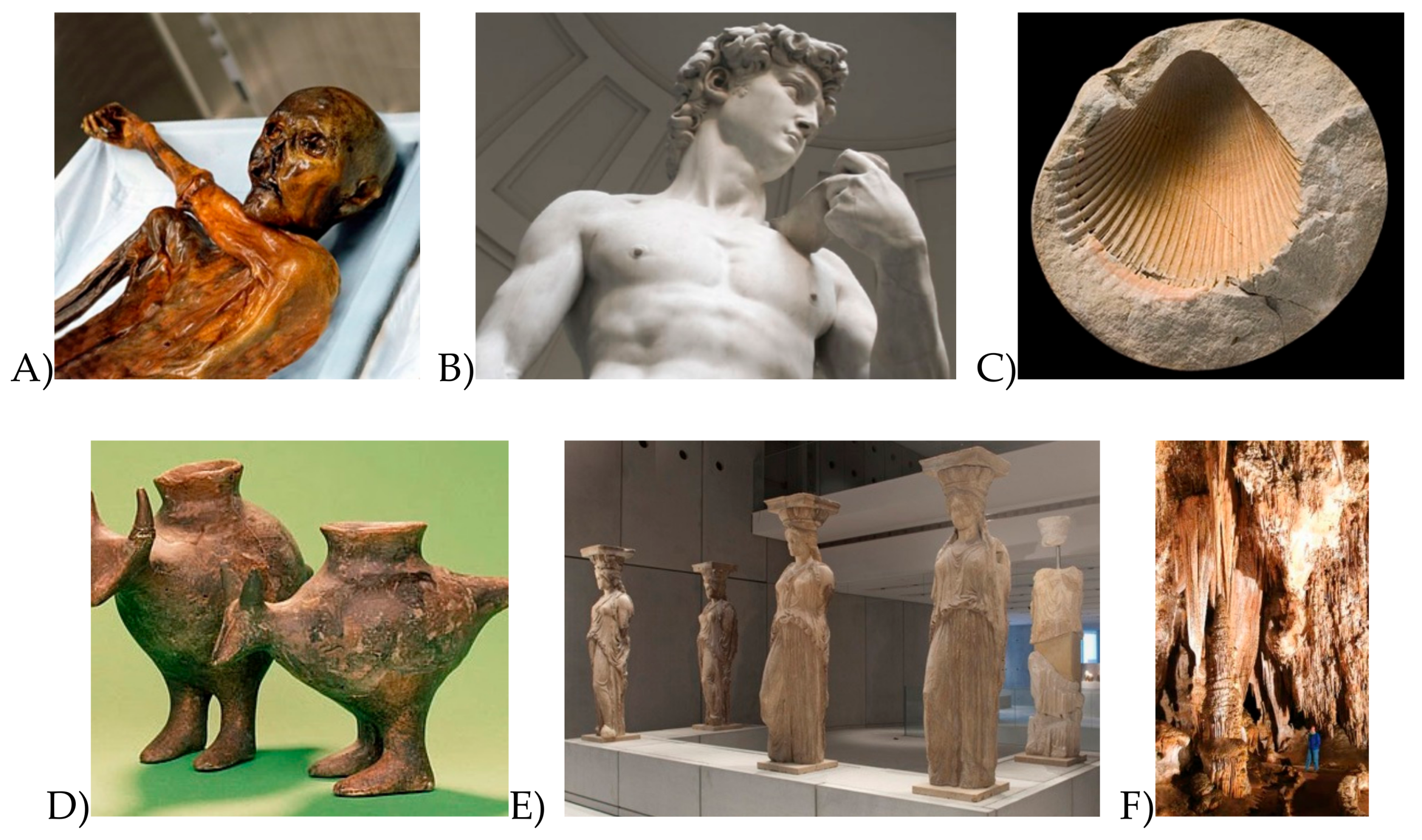
Figure 3.
Examples of natural and man-made geometric (inorganic) shapes: (A) Guggenheim Museum, (B) Filarete Tower in Milan–source www.milanocastello.it, (C) Amethyst-source Amethyst Welt Maissau.
Figure 3.
Examples of natural and man-made geometric (inorganic) shapes: (A) Guggenheim Museum, (B) Filarete Tower in Milan–source www.milanocastello.it, (C) Amethyst-source Amethyst Welt Maissau.

Figure 4.
The dragon dataset downloaded from the Stanford 3D Scanning Repository.
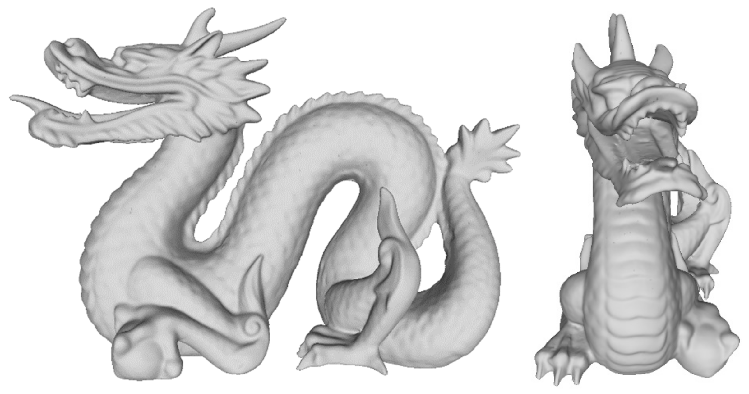
Figure 5.
The multistep workflow for the generation of a solid B-rep model for FEA.
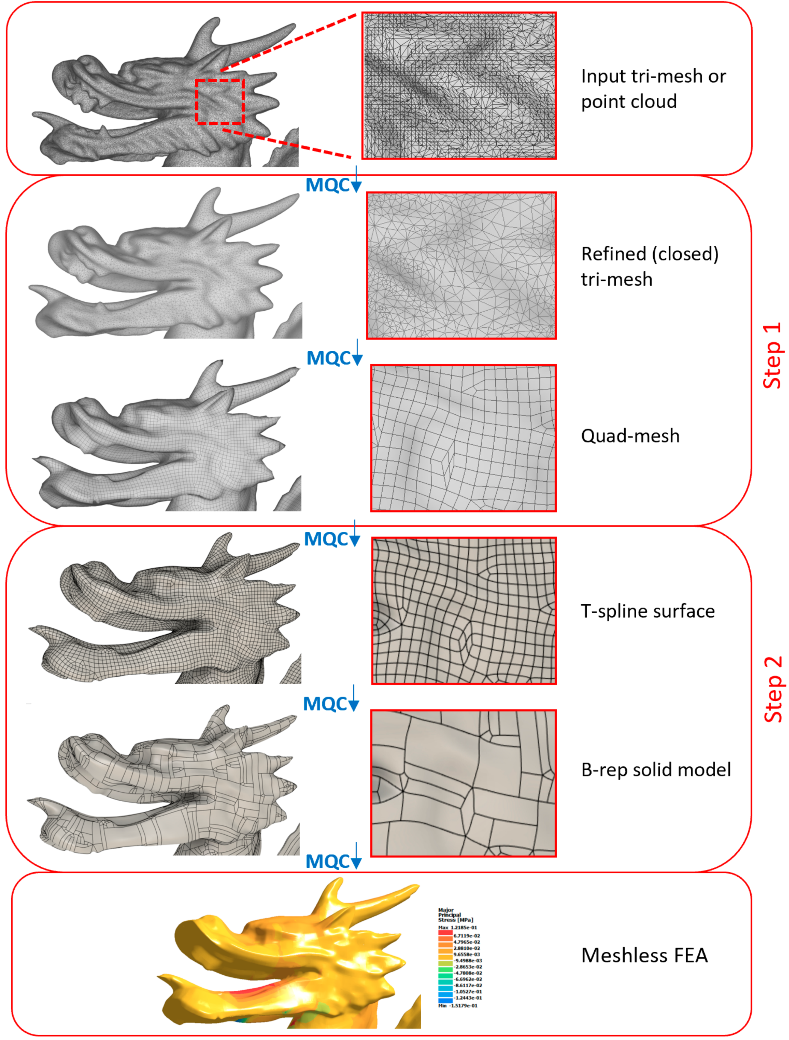
Figure 6.
Detail of the original tri-mesh (A) and the results after removing holes and self-intersections (B). A reduction of triangles and global smoothing filters were applied to get a more uniform surface, reducing creased edges and spikes. The bottom image (C) shows the metric discrepancy in meters between the refined tri-mesh and the original one. The relative RMS is 0.22%.
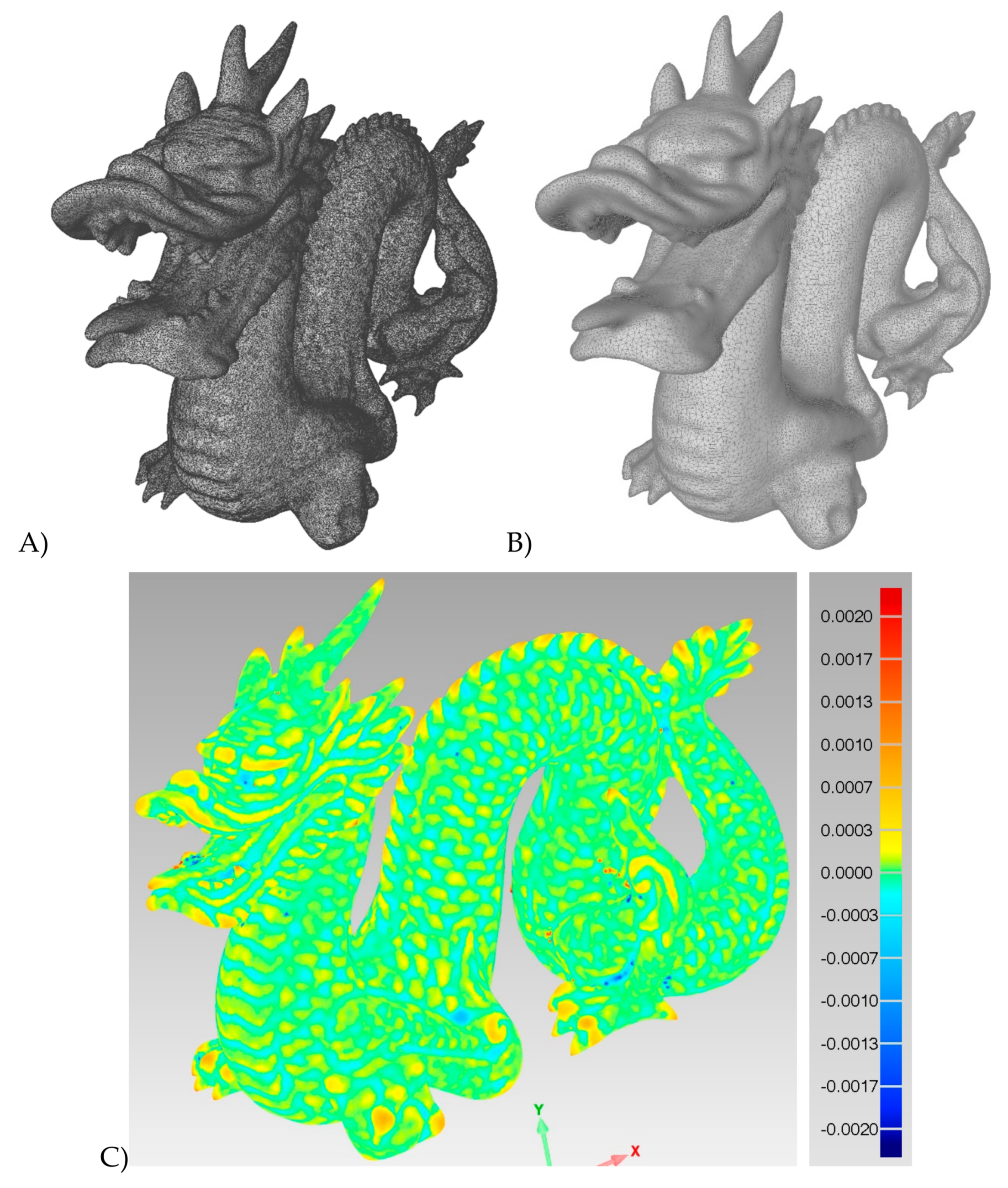
Figure 7.
The different steps for the creation of a quad-mesh: (A) orientation field computation, (B) position field optimization and (C) pure quadrilateral mesh extraction.
Figure 7.
The different steps for the creation of a quad-mesh: (A) orientation field computation, (B) position field optimization and (C) pure quadrilateral mesh extraction.

Figure 8.
The geometric discrepancy in meters between the original tri-mesh and the quad-mesh. The relative RMS is 0.22%.
Figure 8.
The geometric discrepancy in meters between the original tri-mesh and the quad-mesh. The relative RMS is 0.22%.
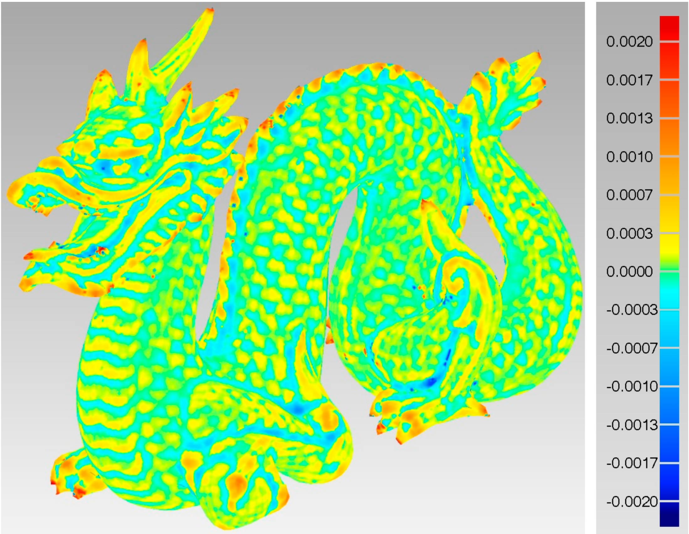
Figure 9.
The decimated tri-mesh with 20,000 faces (i.e., a surface model) and the solid model achieved with a direct conversion. The solid exactly replicates the structure of the mesh and has a clear tessellation in a large number of small elements.
Figure 9.
The decimated tri-mesh with 20,000 faces (i.e., a surface model) and the solid model achieved with a direct conversion. The solid exactly replicates the structure of the mesh and has a clear tessellation in a large number of small elements.

Figure 10.
: Tri-mesh with 1000 faces representing a unary sphere (R = 1 m) with an RMS of 0.0015 m (A). Quad-ball generated using T-splines converted into a B-rep solid model requires just 24 faces to get a similar RMS of 0.0014 m (B). The error scale is in meters.
Figure 10.
: Tri-mesh with 1000 faces representing a unary sphere (R = 1 m) with an RMS of 0.0015 m (A). Quad-ball generated using T-splines converted into a B-rep solid model requires just 24 faces to get a similar RMS of 0.0014 m (B). The error scale is in meters.
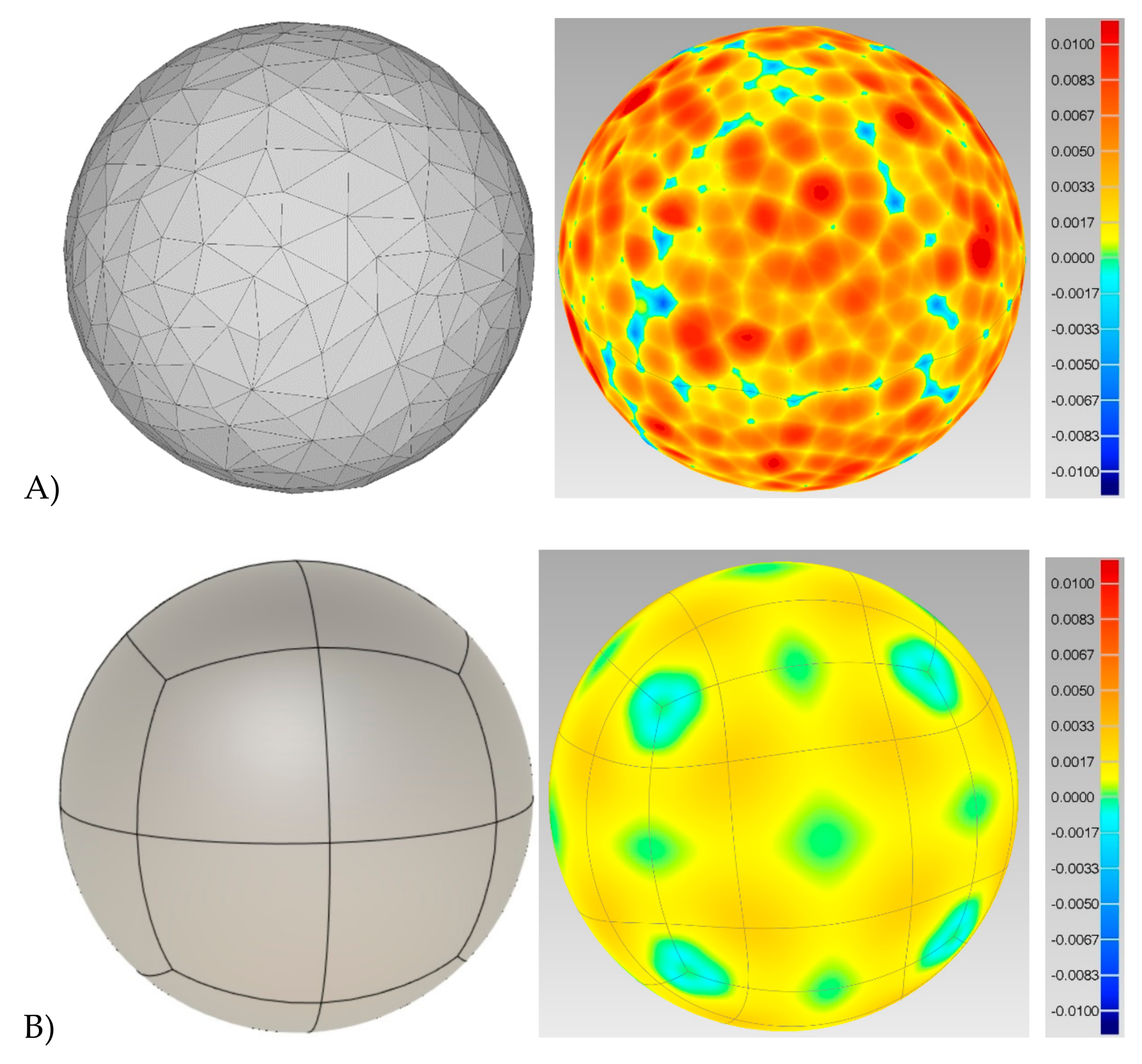
Figure 11.
Example of issues consisting of problematic star-points automatically detected in the T-splines model (A), and a detail of the tail (B).
Figure 11.
Example of issues consisting of problematic star-points automatically detected in the T-splines model (A), and a detail of the tail (B).
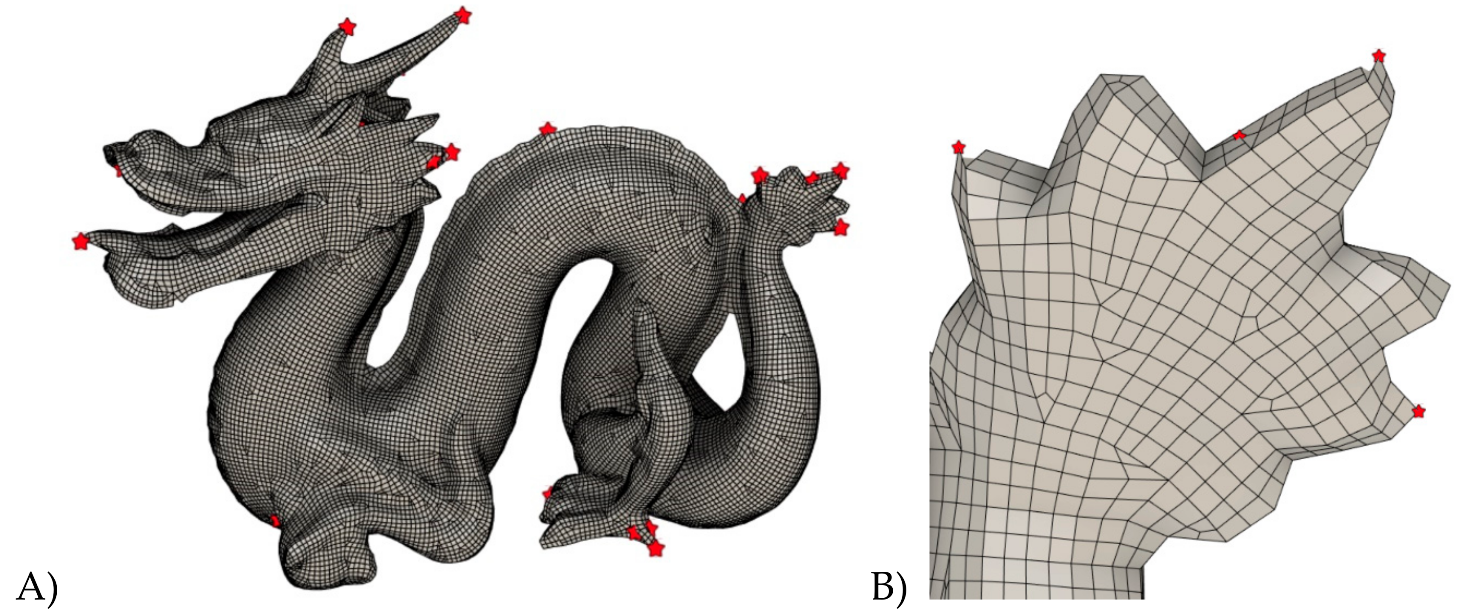
Figure 12.
The removal of star-points was carried out using automatic detection and correction algorithms, obtaining a closed topologically corrected T-spline surface which can be converted into a B-rep solid (A), and a detail of the tail (B).
Figure 12.
The removal of star-points was carried out using automatic detection and correction algorithms, obtaining a closed topologically corrected T-spline surface which can be converted into a B-rep solid (A), and a detail of the tail (B).

Figure 13.
The final B-rep solid generated with the conversion of the T-splines into watertight NURBS patches (A), and a detail of the tail (B). The geometric discrepancy in meters of the solid compared to the initial tri-mesh is RMS = 0.0005m (C), that is a relative error of about 0.18%.
Figure 13.
The final B-rep solid generated with the conversion of the T-splines into watertight NURBS patches (A), and a detail of the tail (B). The geometric discrepancy in meters of the solid compared to the initial tri-mesh is RMS = 0.0005m (C), that is a relative error of about 0.18%.
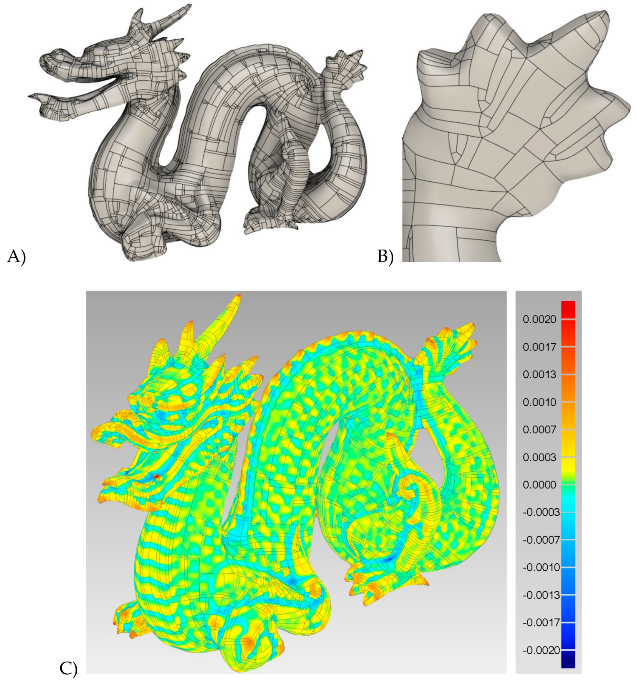
Figure 14.
The solid mesh generated in SimScale that follows the subdivision of the NURBS patches. (A): original B-rep solid model, (B): the solid mesh with tetrahedrons obtained with SimScale, (C): calculation and visualization of the aspect ratio to evaluate solid mesh quality.
Figure 14.
The solid mesh generated in SimScale that follows the subdivision of the NURBS patches. (A): original B-rep solid model, (B): the solid mesh with tetrahedrons obtained with SimScale, (C): calculation and visualization of the aspect ratio to evaluate solid mesh quality.

Figure 15.
(A) Meshless FEA with SimSolid allows one to define boundary conditions of specific parts of surfaces, removing the problem related to the irregular distribution of the NURBS patches. (B) and (C) shows the distribution of the major principal stress.
Figure 15.
(A) Meshless FEA with SimSolid allows one to define boundary conditions of specific parts of surfaces, removing the problem related to the irregular distribution of the NURBS patches. (B) and (C) shows the distribution of the major principal stress.
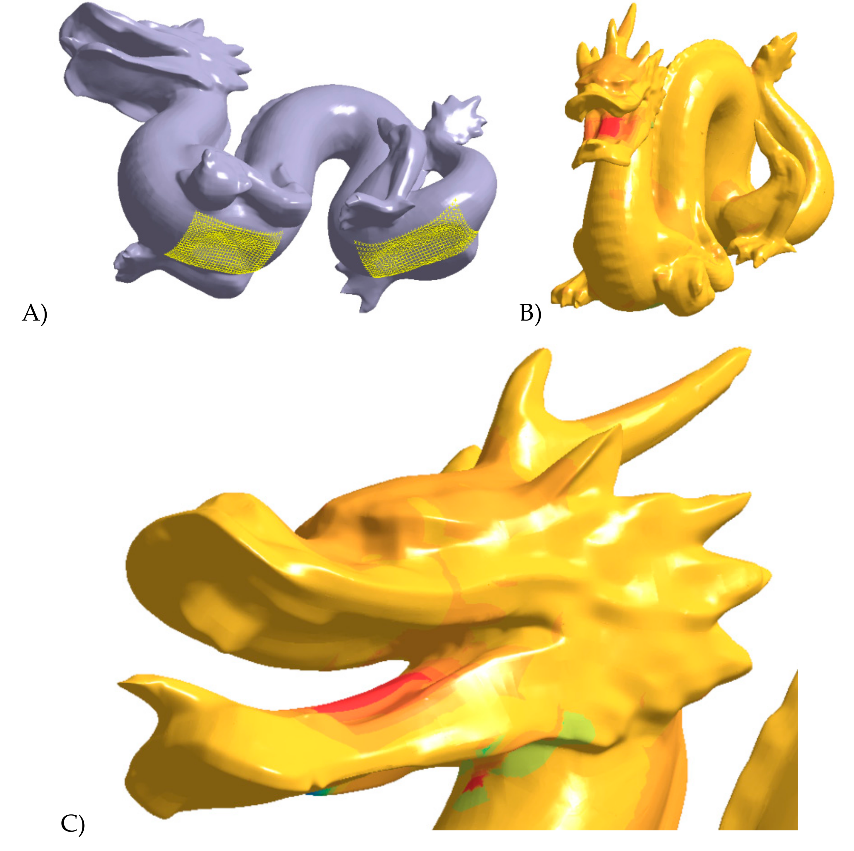
Figure 16.
The initial model synthetically generated (B-rep1 - left) and one of the B-rep2 models (right) reconstructed with the proposed procedure after converting B-rep1 into a surface tri-mesh (in this case the quad-mesh has 9676 vertices).
Figure 16.
The initial model synthetically generated (B-rep1 - left) and one of the B-rep2 models (right) reconstructed with the proposed procedure after converting B-rep1 into a surface tri-mesh (in this case the quad-mesh has 9676 vertices).
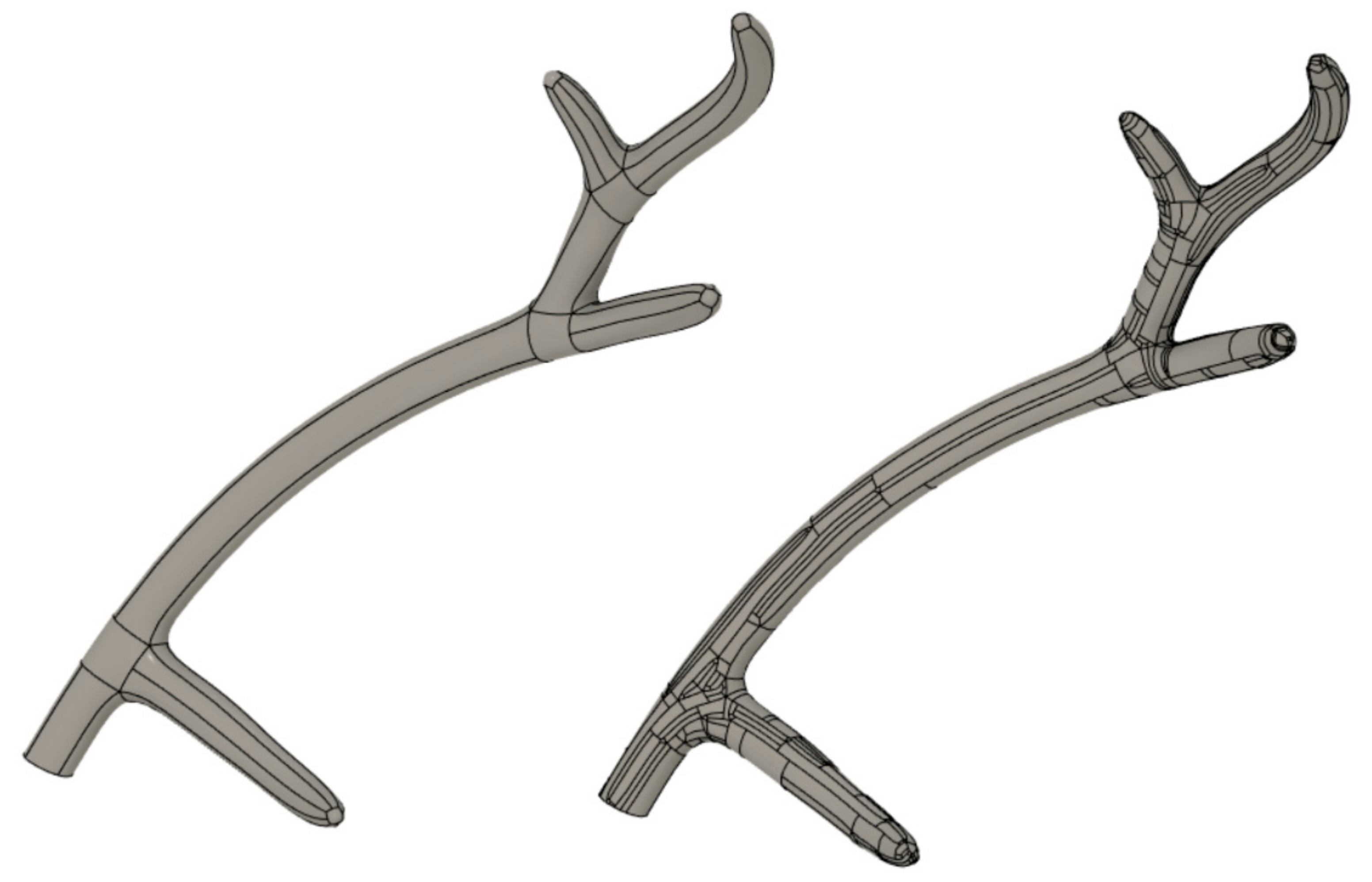
Figure 17.
A detail of the different quad-meshes with a variable resolution. From left to right 50,422– 29,404–14,850 and 9676 vertices, respectively.
Figure 17.
A detail of the different quad-meshes with a variable resolution. From left to right 50,422– 29,404–14,850 and 9676 vertices, respectively.
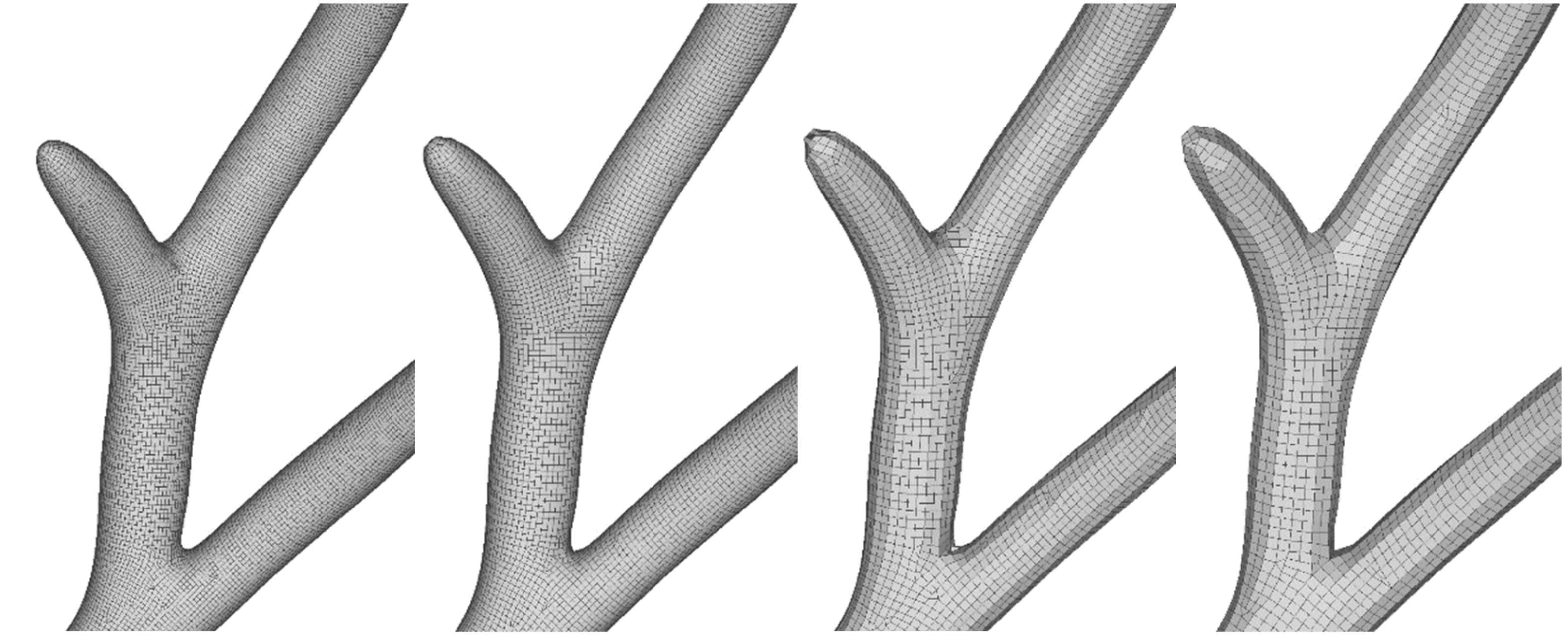
Figure 18.
The geometric discrepancy in millimeters for the 4 different models (B-rep2) compared to the initial model (B-rep1) generated with manual modeling.
Figure 18.
The geometric discrepancy in millimeters for the 4 different models (B-rep2) compared to the initial model (B-rep1) generated with manual modeling.

Figure 19.
Loading schemes with Solid Edge (A) and Solidworks (B). Visualization of the displacement maps calculated with different software using the B-rep1 model: Solid Edge (C), SimScale (D), Solidworks (E) and SimSolid (F).
Figure 19.
Loading schemes with Solid Edge (A) and Solidworks (B). Visualization of the displacement maps calculated with different software using the B-rep1 model: Solid Edge (C), SimScale (D), Solidworks (E) and SimSolid (F).

Figure 20.
The general scheme of the experiment (A) and preliminary tri-mesh (B) generated from the B-rep1 solid model used to produce the B-rep2 solids.
Figure 20.
The general scheme of the experiment (A) and preliminary tri-mesh (B) generated from the B-rep1 solid model used to produce the B-rep2 solids.
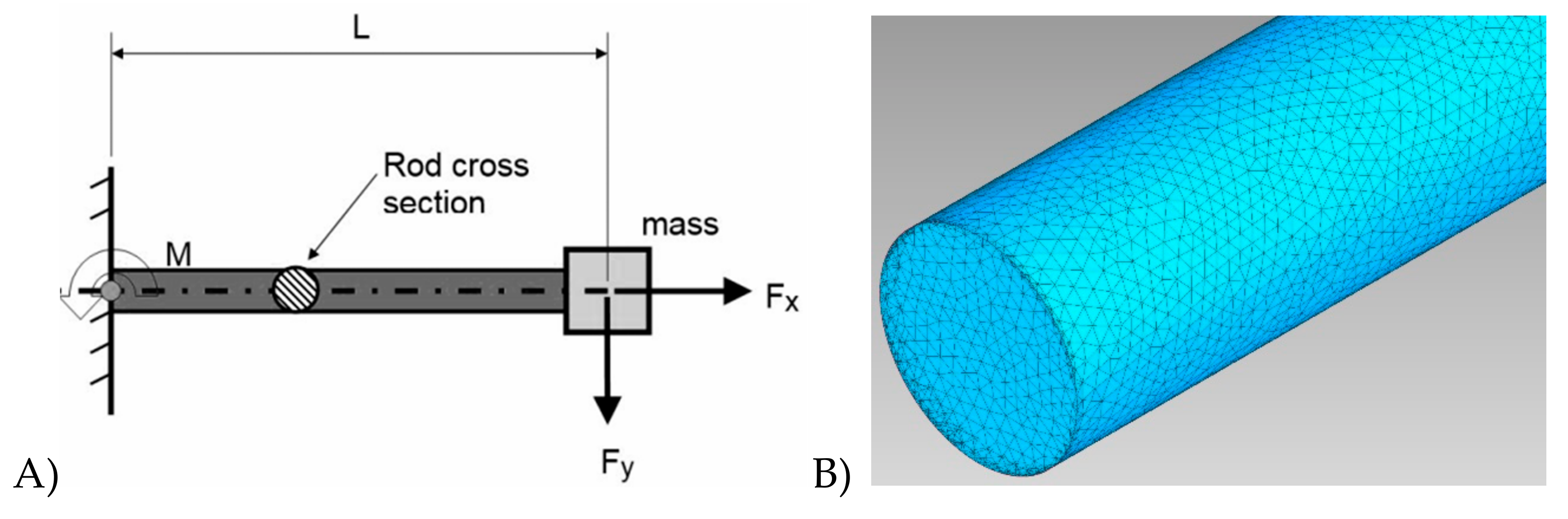
Figure 21.
A simple geometry like a cylindrical rod can be turned into a quad-surface with an inhomogeneous quad-density. (A) and (B) shows a uniform pattern, in the (C) case a star point will probably appear, resulting in a subdivision of NURBS patches.
Figure 21.
A simple geometry like a cylindrical rod can be turned into a quad-surface with an inhomogeneous quad-density. (A) and (B) shows a uniform pattern, in the (C) case a star point will probably appear, resulting in a subdivision of NURBS patches.

Figure 22.
Different processing steps for the Statue of Asclepius (the reader is referred to the text for a description of the different pictures).
Figure 22.
Different processing steps for the Statue of Asclepius (the reader is referred to the text for a description of the different pictures).

Figure 23.
Different processing steps for the Bust of Augustus (the reader is referred to the text for a description of the different pictures). The error scale is in meters.
Figure 23.
Different processing steps for the Bust of Augustus (the reader is referred to the text for a description of the different pictures). The error scale is in meters.

Figure 24.
Different processing steps for the Coptic capital (the reader is referred to the text for a description of the different pictures).
Figure 24.
Different processing steps for the Coptic capital (the reader is referred to the text for a description of the different pictures).
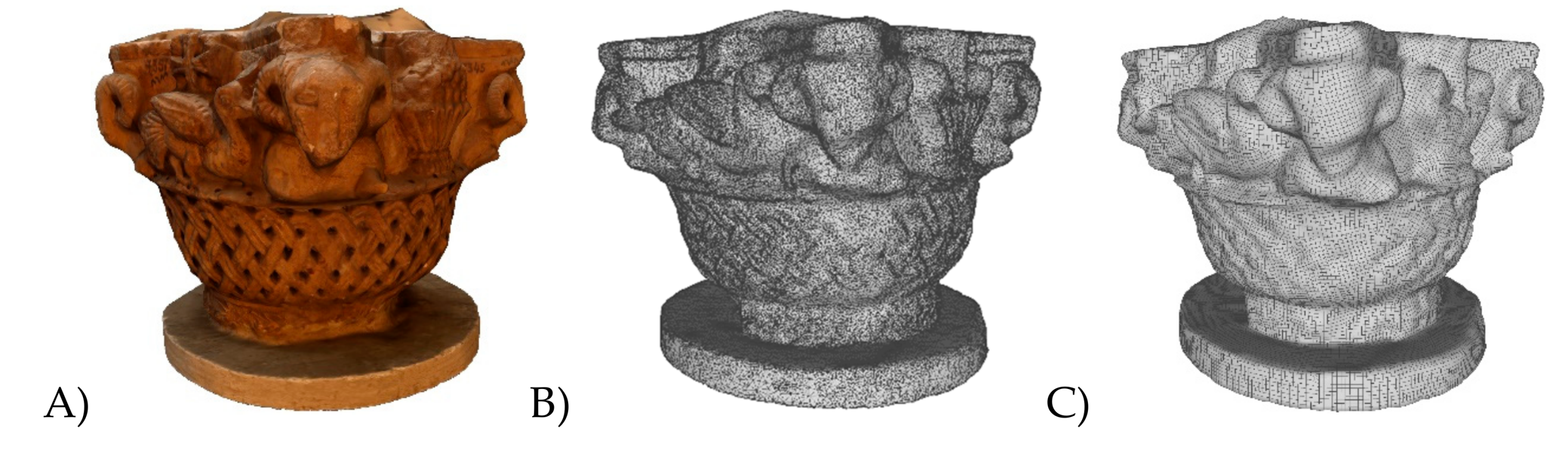


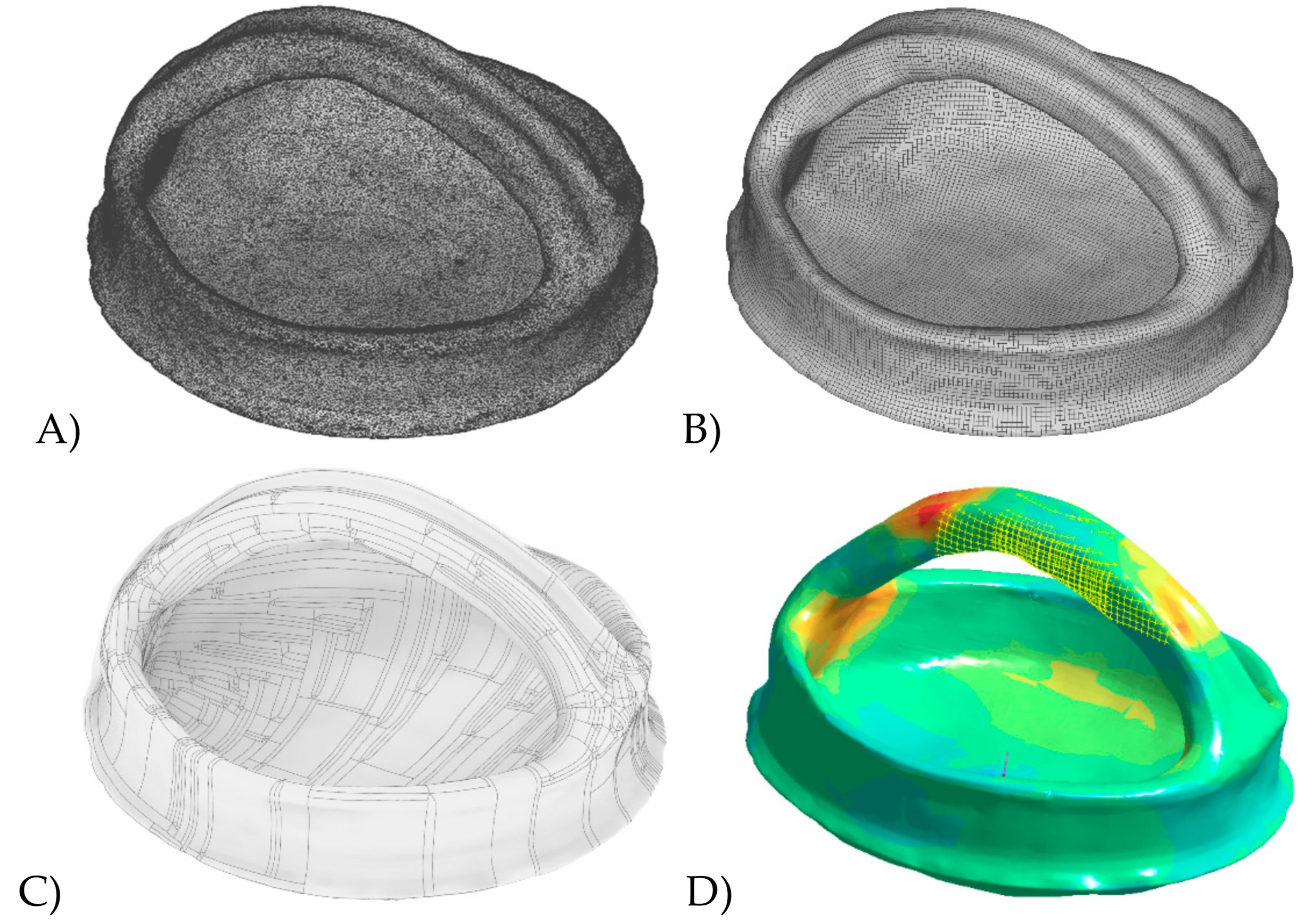
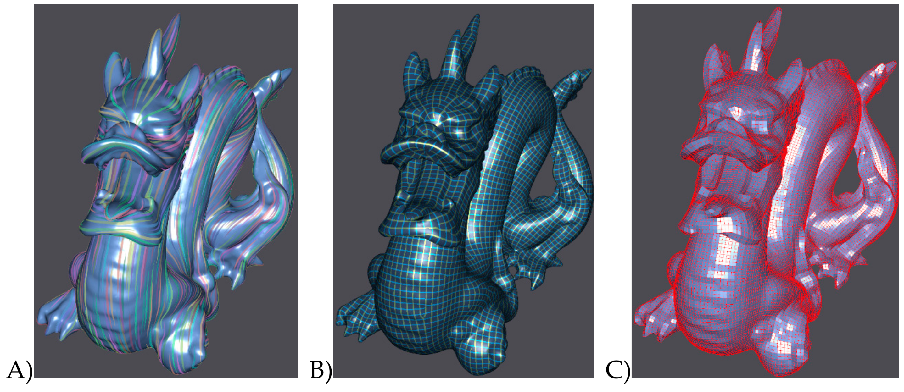
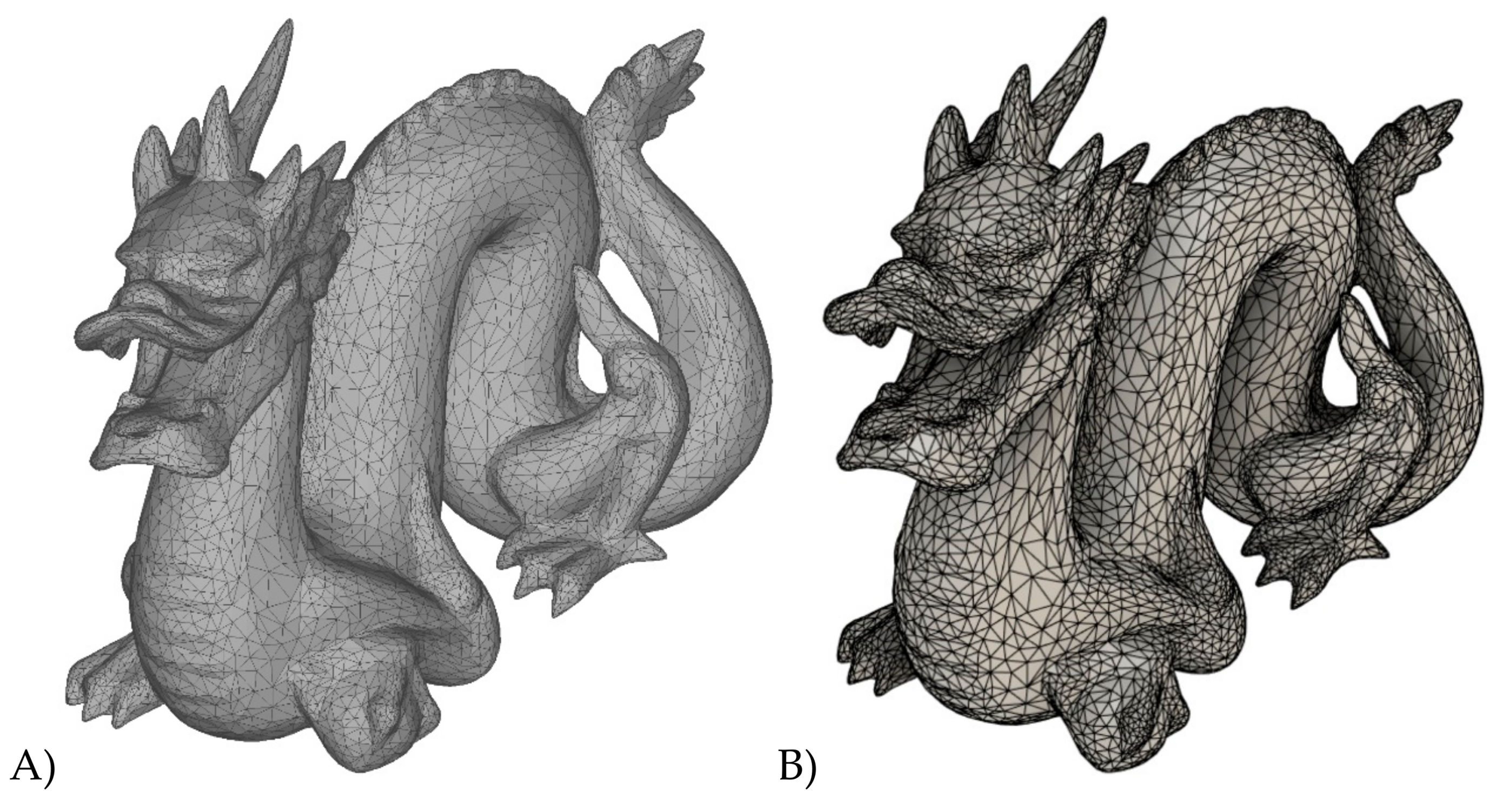
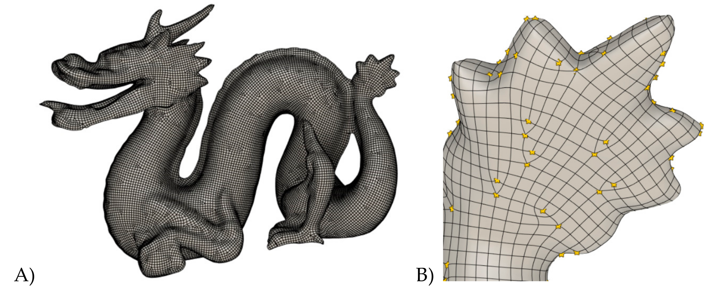
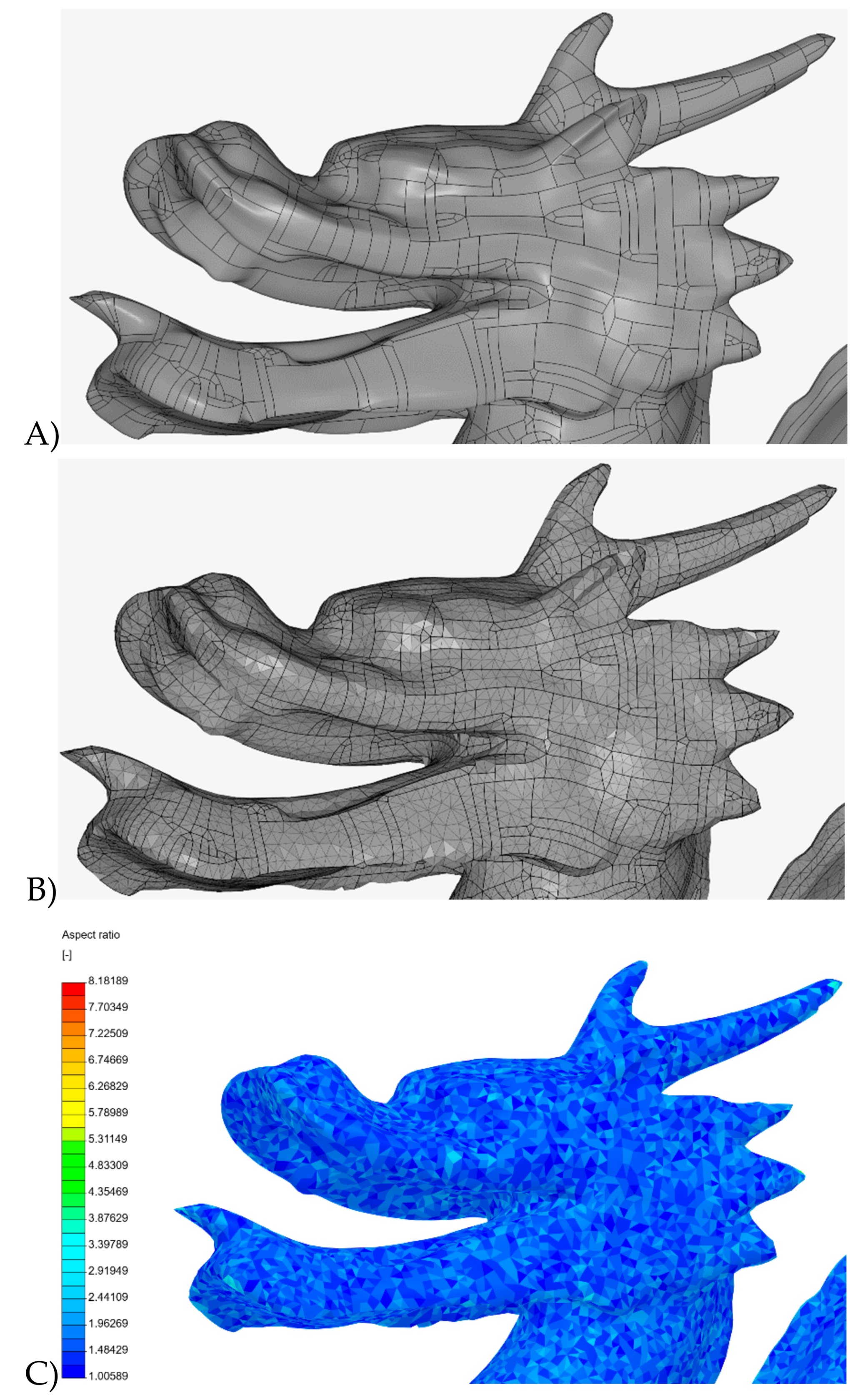
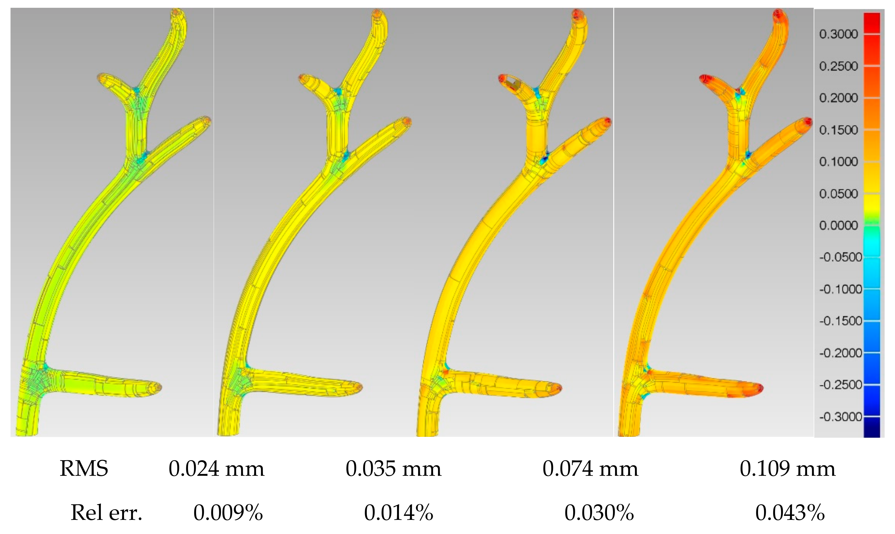
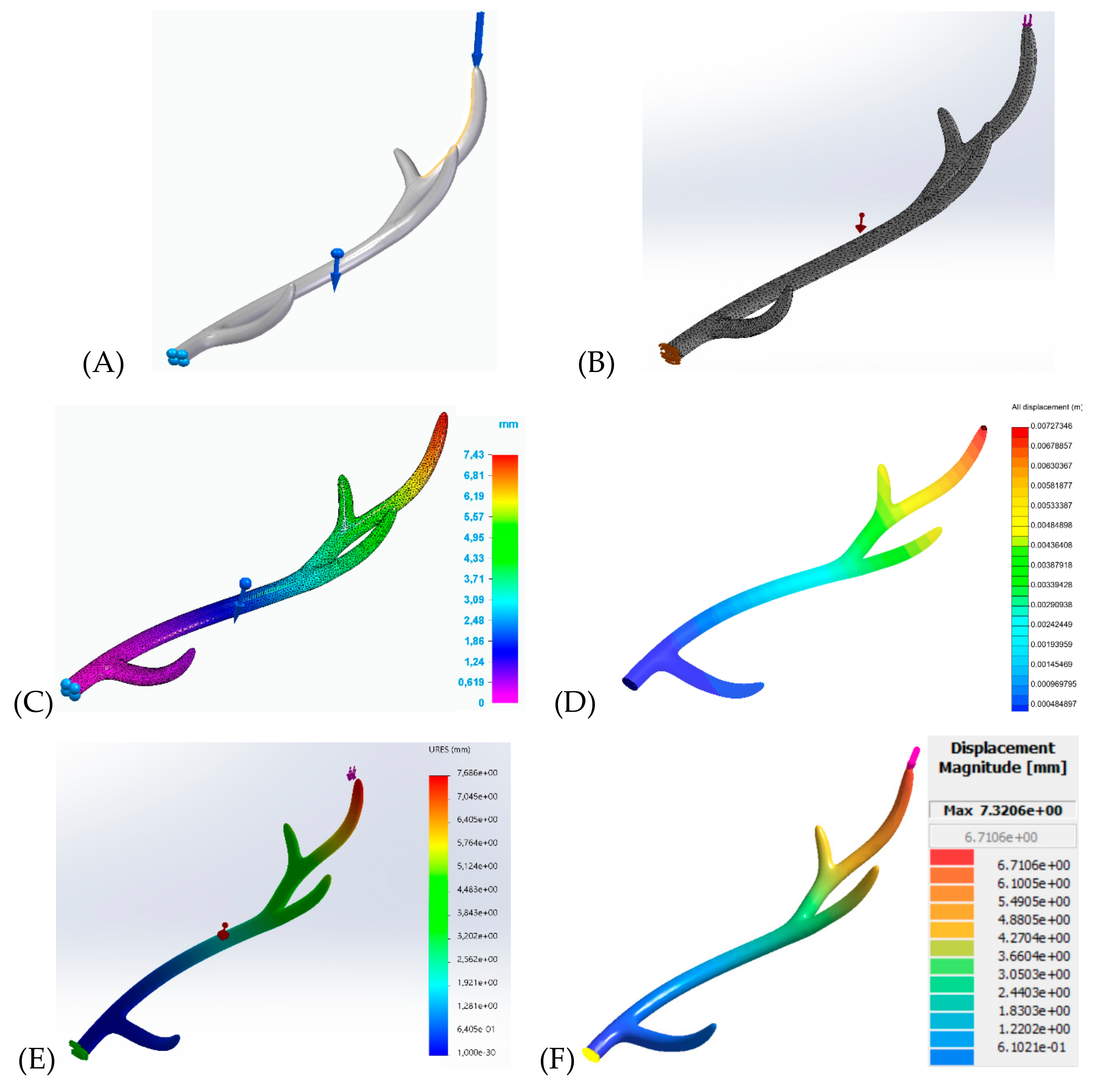
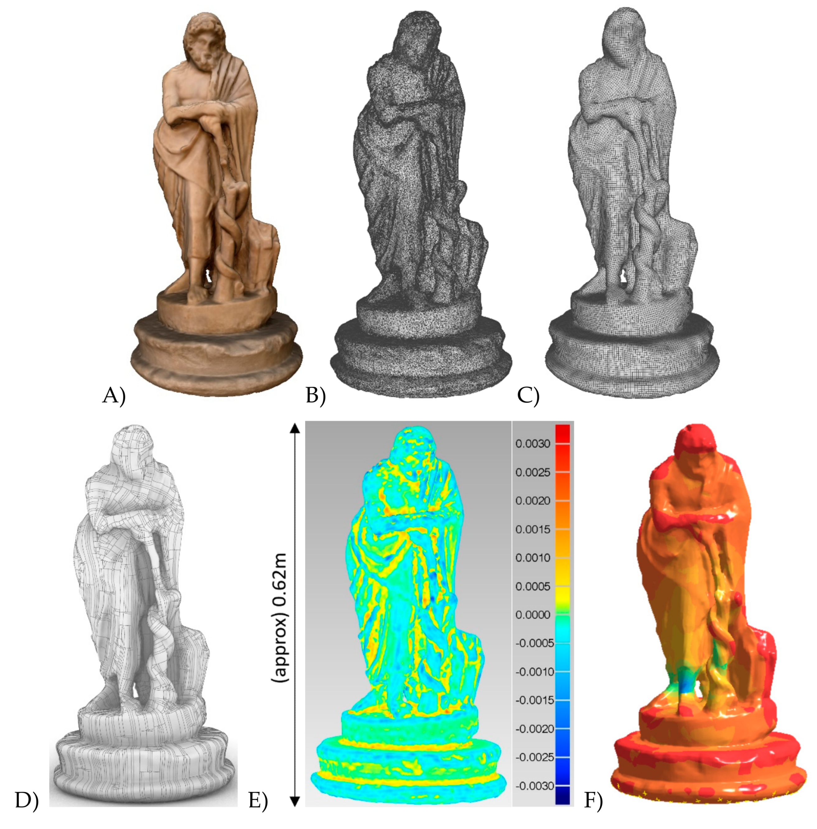
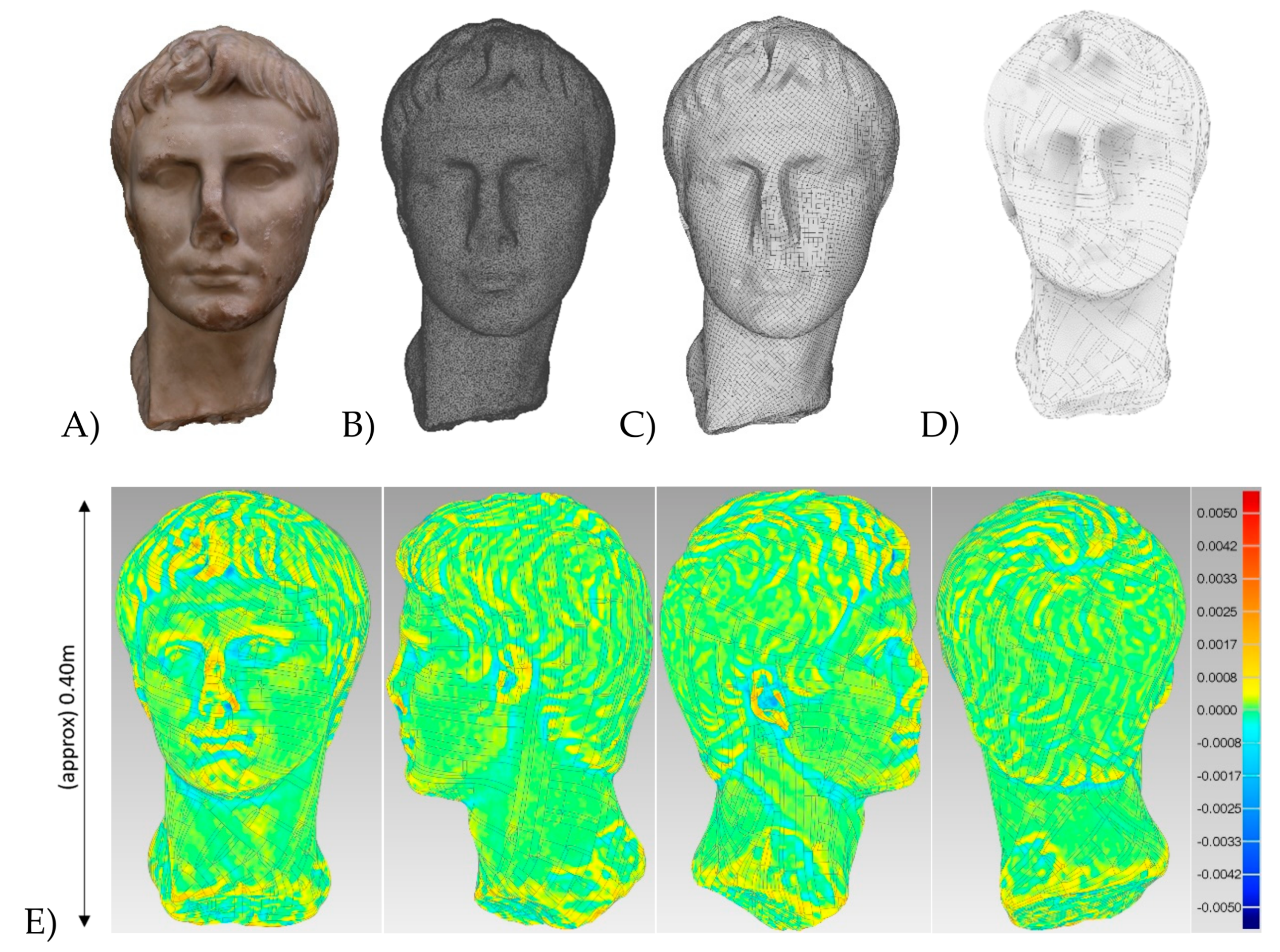
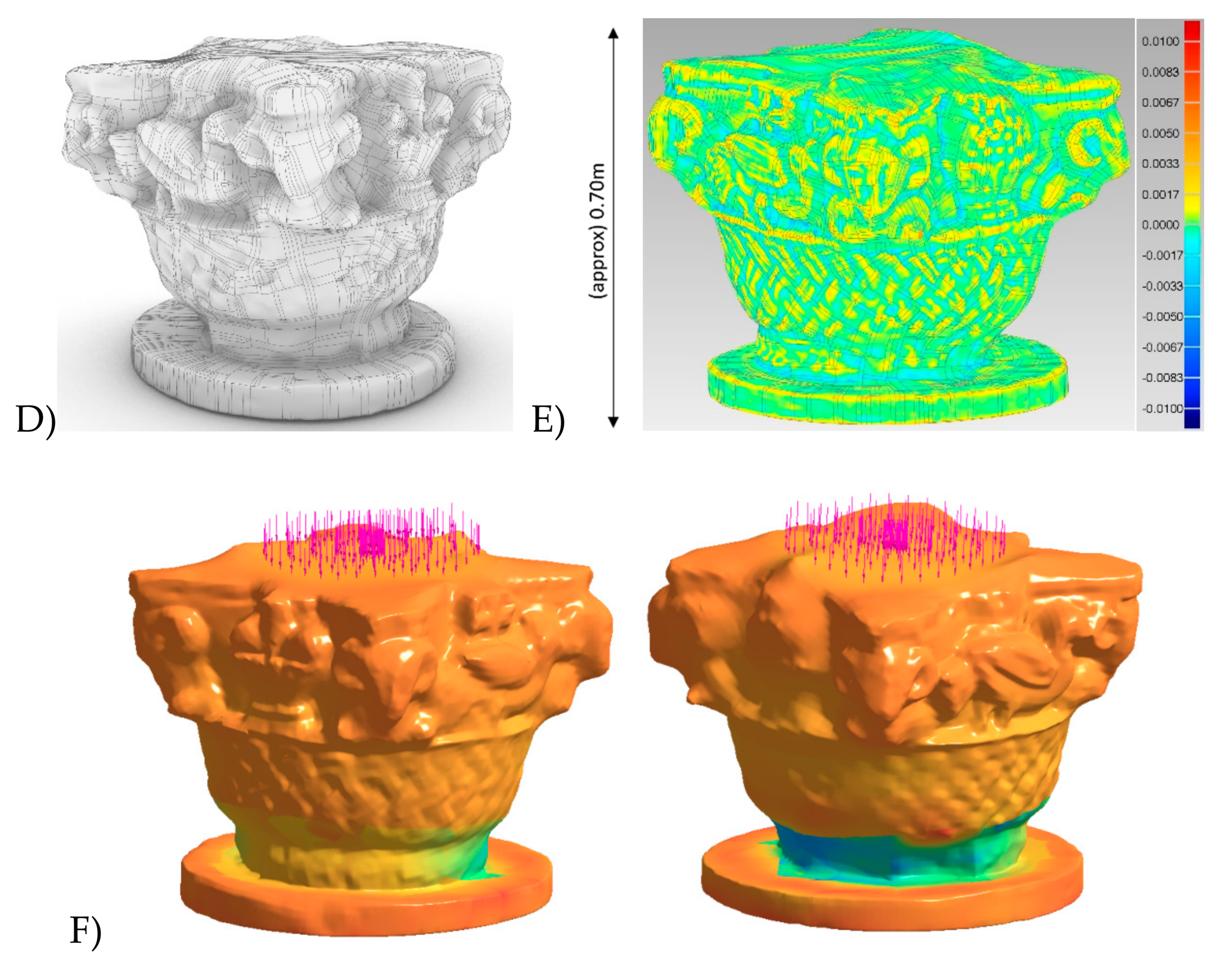
Table 1.
Maximum deflection calculated with the original STEP model (B-rep1) and different software compared to the regenerated models (B-rep2) with variable resolutions and the meshless FEA approach.
Table 1.
Maximum deflection calculated with the original STEP model (B-rep1) and different software compared to the regenerated models (B-rep2) with variable resolutions and the meshless FEA approach.
| Type of Model | Max Displacement Calculated with Different Software (mm) | |||
|---|---|---|---|---|
| SimSolid | SolidEdge | SimScale | Solidworks | |
| B-rep1 (original) | 7.3 | 7.4 | 7.3 | 7.7 |
| B-rep2 (50,422 vertices) | 7.4 | - | - | - |
| B-rep2 (29,404 vertices) | 7.4 | - | - | - |
| B-rep2 (14,850 vertices) | 7.6 | - | - | - |
| B-rep2 (9676 vertices) | 7.7 | - | - | - |
Table 2.
Comparison of the maximum Von Mises stress computed with the original B-rep1 model and different software and the result of meshless FEA with the reconstructed B-rep2 models with different resolutions of the quad-mesh.
Table 2.
Comparison of the maximum Von Mises stress computed with the original B-rep1 model and different software and the result of meshless FEA with the reconstructed B-rep2 models with different resolutions of the quad-mesh.
| Type of Model | Max Von Mises Stress Calculated with Different Software (MPa) | |||
|---|---|---|---|---|
| SimSolid | SolidEdge | SimScale | Solidworks | |
| B-rep1 (original) | 165 | 164 | 162 | 165 |
| B-rep2 (32,670 vertices) | 168 | - | - | - |
| B-rep2 (16,804 vertices) | 171 | - | - | - |
| B-rep2 (9234 vertices) | 174 | - | - | - |
© 2020 by the author. Licensee MDPI, Basel, Switzerland. This article is an open access article distributed under the terms and conditions of the Creative Commons Attribution (CC BY) license (http://creativecommons.org/licenses/by/4.0/).
Share and Cite
MDPI and ACS Style
Barazzetti, L. Solid Model Generation for Digitized Organic Bodies via T-Splines. Heritage 2020, 3, 606-636. https://doi.org/10.3390/heritage3030035
AMA Style
Barazzetti L. Solid Model Generation for Digitized Organic Bodies via T-Splines. Heritage. 2020; 3(3):606-636. https://doi.org/10.3390/heritage3030035
Chicago/Turabian StyleBarazzetti, Luigi. 2020. "Solid Model Generation for Digitized Organic Bodies via T-Splines" Heritage 3, no. 3: 606-636. https://doi.org/10.3390/heritage3030035