Enhancing Methods for Grid-Load Forecasting in Order to Reduce Grid Losses

Highlights

What are the main findings?

• A comprehensive evaluation of 14 statistical, machine learning, and hybrid forecasting models is conducted on unique quarter-hourly substation-level load data, showing that models incorporating lagged variables and exogenous inputs (weather, temporal indicators) substantially outperform all non-lagged counterparts across MAE, RMSE, and MAPE metrics.
• A hybrid averaging model combining OLS, XGBoost, and Feedforward Neural Networks achieves the strongest forecasting accuracy, reducing MAE from 4.55 to 1.61 kWh relative to the standard correction method currently used by Dutch grid operators, with improvements confirmed by paired t-tests and the Diebold–Mariano test.

What are the implications of the main findings?

• Substation-level, data-driven load forecasting significantly sharpens the deviation signals used to detect grid losses from electricity theft, defective meters, and cable faults, enabling grid operators to intervene earlier and more precisely.
• Replacing aggregated correction factors with advanced forecasting pipelines trained on granular, location-specific data is practically feasible—models require infrequent retraining and generate predictions in under five seconds—offering a scalable upgrade path for distribution system operators.

Abstract

Accurate forecasting of electrical load at the substation level is essential for detecting grid losses that pose significant financial and safety challenges. This study investigates whether the standard correction method currently used by grid operators can be improved through the application of advanced forecasting models to granular, location-specific load data. Such improvements are particularly valuable for identifying abnormal consumption patterns indicative of grid losses due to electricity theft, defective meters, or cable damage. This paper evaluates a broad range of statistical and machine learning models—including ARIMAX, SARIMAX, Random Forests, Gradient Boosting Machines, Neural Networks, and Support Vector Regression—based on unique quarter-hourly datasets from several Dutch substations. Two hybrid approaches are proposed, combining the best-performing individual models through a stacked ensemble method and a simpler averaging strategy. The results show that incorporating lagged and additional exogenous variables, along with the application of various advanced models, significantly improves forecasting accuracy compared to the standard correction method, with the best hybrid model reducing MAE and RMSE by approximately 64.7% and 61.6%, respectively, relative to the current operational benchmark. This study demonstrates that substation-level, data-driven forecasting can strengthen the signals used to detect grid losses, offering practical implications for grid operators and policymakers.

1. Introduction

Grid loss, defined as the discrepancy between the electric energy injected into the grid and the used energy that is billed to end-users, presents a pervasive and complex challenge for grid operators. Accurate forecasting of electricity load at electrical substations is essential to identify and mitigate these losses, thereby reducing financial impacts for both grid operators and retail consumers, as part of these losses are ultimately passed on to end-users. Significant deviations between expected and actual load can indicate grid losses caused by unauthorized usage, such as electricity theft by hemp farms or other illegal activities, as well as by defective meters or damaged cables. Such illegal activities do not only result in financial losses, but they also create significant safety hazards, including fire risks from improperly installed grid connections. These risks become more pressing as such operations are increasingly found in residential areas [1]. In 2022, one of the Netherlands’ major distribution-grid operators, Stedin, reported that approximately 15 percent of its total grid loss—equivalent to 120 million kWh of electricity—could be attributed to fraud and theft, amounting to an estimated €25 million in damages [2]. Additionally, in the Netherlands, electricity theft was identified in 1060 hemp farms during the same year, where a total of 75 million kWh was stolen. This represents a notable decrease compared to the 111 million kWh stolen in 2021, which was linked to 1800 dismantled farms. However, law enforcement agencies suggest that this decline is likely also attributable to reduced reporting, driven by growing fears of organized crime and its associated risks, such as violent reprisals [3]. This underscores the urgent need for alternative detection methods.

Previous research has explored various aspects of methods to improve grid management and reduce grid losses. Studies on efficient grid management have primarily focused on optimizing energy distribution, often emphasizing the integration of renewable energy sources [4,5]. Additionally, several studies have examined the detection of unauthorized electricity usage, such as theft or fraud, using techniques like anomaly detection and machine learning models [6,7]. These studies underscore the financial and operational impacts of grid losses and highlight the importance of proactive measures. Although load forecasting and ensemble-based methods are well-established in the broader forecasting literature, relatively little work applies these techniques to the operational problem of grid-loss detection at the substation level. Prior studies typically rely on generalized or publicly available datasets, which fail to capture the complex, localized patterns present in real distribution networks [8]. Moreover, most existing studies focus on aggregated demand forecasting for larger networks and longer time horizons, overlooking the fine-grained, short-horizon, location-specific predictions required to identify unauthorized usage, detect anomalies, and support efficient grid operations [9].

To address this gap, this study develops an improved methodology for forecasting electricity load at the substation level. The model currently used by grid operators relies on aggregated historical averages and generalized correction factors, and therefore cannot capture localized patterns or the influence of important explanatory variables. The proposed forecasting framework incorporates commonly used explanatory information in short-term load forecasting, including temporal indicators, weather-related variables, and lagged load values, to construct more accurate expected-load estimates at the substation level. By evaluating whether more sophisticated forecasting techniques can improve the accuracy of expected-load estimates, this study assesses their potential to strengthen the deviation signals that grid operators rely on when identifying possible grid losses. Although forecasting alone does not reduce grid loss directly, improved forecasting accuracy enhances the detection mechanism used by grid operators. When expected load is estimated more precisely, deviations from normal patterns can be identified earlier and more reliably, enabling faster interventions against theft, meter defects, or cable failures, which ultimately helps reduce energy loss in practice.

This study systematically evaluates a broad range of machine learning techniques—including Random Forest, Gradient Boosting Machines, and Neural Networks—alongside traditional statistical approaches such as ARIMA and SARIMA, as well as the model currently employed by grid operators. In addition, two novel hybrid models were developed: a complex stacked ensemble model and a simpler averaging method, both leveraging the strengths of the best-performing individual models, including OLS, Extreme Gradient Boosting (XGBoost), and Feedforward Neural Networks (FNN), all enhanced with lagged variables. This study was made possible through a close collaboration with Dimaros, a company developing algorithms to detect cannabis farms on behalf of the Dutch government, in partnership with the largest grid operators. These partnerships provided access to detailed, location-specific, quarter-hourly electricity load data from several substations in the Netherlands—data that are typically unavailable for public research due to privacy constraints. This data is used to examine the extent to which electricity load forecasts can be improved. Through a systematic comparison using evaluation metrics such as MAE, RMSE, MAPE, and the Diebold–Mariano test [10], the optimal model for substation-level forecasting was identified.

The findings show that incorporating granular, location-specific data and advanced machine learning techniques significantly improves forecasting accuracy compared to the model currently used by grid operators. While training these models can be computationally intensive, this process does not need to be performed frequently. Once the dataset reaches a sufficient size, the models effectively capture load patterns. Additionally, retraining can be performed in the background while the existing model remains operational, ensuring continuous forecasting availability.

This paper makes three key contributions to the literature:

• This study introduces a unique real-world dataset containing quarter-hourly, substation-level load measurements from a major Dutch distribution system operator. Such granular operational data is rarely available in forecasting research and enables the incorporation of richer explanatory variables—including weather conditions, temporal indicators, and lagged load patterns—that are absent from the forecasting method currently used by grid operators.
• An underexplored question in the literature is addressed by examining whether improved short-horizon forecasts can enhance grid loss detection, a task traditionally based on aggregated historical averages rather than predictive modeling. The expanded feature set enables the first quantitative evaluation of how advanced forecasting methods compare with the traditional model, demonstrating substantial and statistically significant reductions in forecasting error.
• This study provides the most comprehensive assessment to date of forecasting techniques for substation-level load prediction, evaluating 14 statistical, machine learning, and hybrid models under a unified methodological framework that includes out-of-sample overfitting diagnostics and Diebold–Mariano significance testing.

The remainder of this paper is structured as follows: Section 2 provides a comprehensive review of the existing literature, contextualizing the study within the broader body of research. Section 3 details the methodologies employed, including the evaluation metrics. Section 4 describes the datasets utilized in this study, highlighting their characteristics. Section 5 presents the results of the analysis, offering insights into the comparative performance of the models. Section 6 discusses the limitations of the study and suggests potential directions for future research. Finally, Section 7 concludes the paper by summarizing the key findings.

2. Literature Review

Electricity load forecasting has been widely studied across both transmission and distribution systems, resulting in a broad range of methodological approaches. The literature spans traditional statistical models, machine learning techniques, and hybrid frameworks designed to capture complex temporal and nonlinear patterns. This section reviews the main forecasting methods used in prior research, highlighting their capabilities and limitations in the context of short-term electricity load prediction.

A large body of prior work shows that electricity load is strongly influenced by weather conditions such as temperature and sunshine, temporal variables such as hour-of-day, day-of-week, and holidays, and by past load values capturing autocorrelation patterns [11,12,13]. The independent variables used in this study are selected in line with this literature and are chosen to capture location-specific, substation-level temporal and weather-related patterns that define expected electricity consumption.

In parallel, a wide range of time series models has been developed to exploit the temporal structure of electricity load data. Among these, the AutoRegressive Integrated Moving Average with Exogenous Regressors (ARIMAX) and its seasonal extension SARIMAX are frequently applied for short-term load forecasting, particularly when data exhibit linear structures [14,15]. However, their performance often declines in the presence of nonlinearities or complex seasonal behavior. In response to such limitations, alternative statistical models have been developed. For instance, a recent study found that Prophet, a model developed by Facebook, provided superior one-day-ahead load forecasts in scenarios where seasonality and trend variations were more complex [16].

In recent years, machine learning models have gained significant traction in the forecasting domain. Neural networks have been used not only for load forecasting but also for fraud detection using smart meter data [17,18]. Deep learning methods [19], including Feedforward Neural Networks (FNN) [20], have shown strong predictive performance. Similarly, k-Nearest Neighbor (kNN) has been shown to accurately forecast daily residential load, highlighting the versatility of non-parametric models [21]. Beyond Neural Networks, Support Vector Machines (SVM) and their regression counterpart SVR have also proven effective in diverse forecasting applications, including building-level forecasting [22,23]. Moreover, Least Squares SVMs were found to outperform other machine learning approaches in a case study on forecasting hourly residential electricity use, demonstrating their robustness [24]. Tree-based methods have similarly received considerable attention, in part because of their flexibility and accuracy. Decision trees can outperform more complex models such as Neural Networks [25]. Building on this foundation, ensemble methods such as Random Forests and Bagging Regression have delivered strong results across different electricity forecasting contexts [26,27,28]. Even more advanced are Gradient Boosting techniques, including XGBoost, which have demonstrated particularly strong performance in both residential forecasting and electric vehicle load prediction [27,29,30].

In addition to these traditional machine learning approaches, recent work has applied advanced deep learning and Transformer-based architectures to electrical load forecasting across multiple grid levels. For example, several Transformer models have been benchmarked against established deep learning and machine learning methods on large, publicly available datasets for transmission, low-voltage feeder, and client-level loads, showing that Transformer-based approaches can reduce forecast errors significantly compared to strong non-Transformer baselines [31]. Moreover, a Transformer-based deep probabilistic network for load forecasting has reported improved accuracy as well as richer uncertainty quantification for aggregated load series [32]. These studies demonstrate the potential of Transformer architectures for smart-grid forecasting when extensive public data and high-performance computing resources are available, but they also involve complex architectures and hyperparameter optimization pipelines, which can be less efficient for operational purposes. In contrast, the present study focuses on models that are more readily implementable within grid operator workflows and offer a transparent and operationally realistic starting point for grid-loss detection at the substation level.

To further enhance accuracy, hybrid models—combinations of statistical and machine learning techniques—have been proposed. For instance, a hybrid model combining a Convolutional Neural Network (CNN) with a multi-layer bidirectional long short-term memory (LSTM) network demonstrated improved forecasting accuracy compared to individual models [33]. Similarly, ARIMA-SVR and ARIMA-RNN hybrids have been proposed for wind speed forecasting, showing better performance than their individual components [34]. Despite the promising results of these various techniques, their application to grid loss detection and large-scale operational planning poses challenges, particularly in terms of computational demands and the risk of overfitting.

Overall, the existing literature provides a rich foundation of forecasting techniques, ranging from classical statistical models to advanced machine learning and hybrid approaches. However, most prior studies focus on aggregated or residential-level demand and evaluate models under theoretical or controlled settings. Far fewer studies examine forecasting performance using high-resolution substation-level data, which are often restricted due to operational sensitivity and privacy considerations, or consider the implications for operational decision-making within distribution networks. These gaps highlight the need for empirical evaluations based on granular, operational substation-level data, which remains largely unexplored in the existing literature.

3. Methodology

To evaluate the effectiveness of different forecasting techniques in predicting electricity load at the substation level, this section presents a comprehensive comparison of multiple modeling approaches. These include traditional statistical methods such as Ordinary Least Squares (OLS) and time series models, as well as advanced machine learning algorithms and hybrid ensemble techniques. To ensure full reproducibility, all stochastic models were trained using a fixed random seed; preliminary checks confirmed that variability across different seeds was negligible relative to the magnitude of the forecasting errors. Each model is trained and evaluated on the same dataset, with performance assessed through overfitting diagnostics and out-of-sample prediction metrics. By systematically comparing these models, this study aims to identify the most accurate and practical approach for enhancing electricity load forecasts and ultimately reducing grid losses. All forecasts are generated at the quarter-hour level in local Dutch time, using information available up to time t to predict load at $t+15$ min.

3.1. Ordinary Least Squares (OLS) Regression

A baseline for the forecasting framework is established by implementing an Ordinary Least Squares (OLS) regression, a standard linear method that estimates the relationship between electricity load and a set of explanatory variables. The model is specified as

$$\begin{array}{cc}\hfill real\text{\_}{load}_{it}& =X_{it}\beta +{ϵ}_{it},\hfill \end{array}$$

(1)

where $real\text{\_}{load}_{it}$ is the electricity load at time t for substation i, $X_{it}$ represents the matrix of explanatory variables, $\beta$ is the vector of coefficients estimated by Ordinary Least Squares, and ${ϵ}_{it}$ is the error term. Although OLS offers interpretability and computational simplicity, it is limited in capturing nonlinear relationships that are likely present in electricity load data. This motivates the inclusion of more advanced models in the subsequent sections.

3.2. Statistical Time Series Models

Time series models are pivotal for analyzing and forecasting sequentially collected data, a common feature in electricity load studies. Such data inherently exhibit temporal patterns and trends, necessitating the use of specialized time series techniques. These techniques capture the dynamic nature of electricity usage, identifying underlying patterns such as seasonality, cyclical fluctuations, and the influence of external factors.

In this study, three advanced time series methodologies are employed: the AutoRegressive Integrated Moving Average with eXogenous variables model (ARIMAX), the Seasonal ARIMAX model (SARIMAX), and the Prophet model. These models are well-suited for multifaceted analyses, accounting for the internal dynamics of the time series and incorporating external variables that may affect electricity load patterns.

A unique challenge of the dataset is that it consists of multiple non-overlapping time periods from different substations. This structure can complicate time-series analysis, since continuity is typically important for capturing temporal dependencies. Rather than imposing separate adjustments for the discontinuity, the analysis assumes that daily load patterns are sufficiently similar across substations and time periods. To assess generalizability, extensive out-of-sample testing is conducted (see Section 3.6.2).

3.2.1. ARIMAX

The AutoRegressive Integrated Moving Average with Exogenous Regressors (ARIMAX) model is employed to capture temporal dynamics in electricity load while accounting for external influences. ARIMAX extends the classical ARIMA framework by incorporating exogenous variables such as weather and time-based indicators [35]. The model is specified as

$$\begin{array}{cc}\hfill {\Delta }^{d}real\text{\_}{load}_{it}& =X_{it}\beta +{\displaystyle \sum _{j=1}^p}{\varphi }_j{\Delta }^{d}real\text{\_}{load}_{i,t-j}+{\displaystyle \sum _{j=1}^q}{\theta }_j{ϵ}_{i,t-j}+{ϵ}_{it}.\hfill \end{array}$$

(2)

Here, $X_{it}$ denotes the matrix of exogenous regressors and $\beta$ the corresponding coefficients on these regressors. ${\Delta }^d$ represents the differencing operator applied d times to ensure stationarity. The parameters ${\varphi }_j$ and ${\theta }_j$ correspond to the autoregressive (AR) and moving average (MA) components of the model, respectively. The lag orders p, d, and q were selected based on the Akaike Information Criterion (AIC), which penalizes model complexity to avoid overfitting.

3.2.2. SARIMAX

The Seasonal AutoRegressive Integrated Moving Average with Exogenous Regressors (SARIMAX) model extends ARIMAX by including seasonal components to capture recurring patterns in the data [15]. This is particularly relevant for electricity load data, which often exhibits seasonality driven by temperature, daylight variation, and consumer behavior. The SARIMAX model is defined as

$$\begin{array}{cc}\hfill {\Delta }^d{\Delta }_s^{D}real\text{\_}{load}_{it}& =X_{it}\beta +{\displaystyle \sum _{j=1}^p}{\varphi }_j{\Delta }^d{\Delta }_s^{D}real\text{\_}{load}_{i,t-j}+{\displaystyle \sum _{j=1}^q}{\theta }_j{ϵ}_{i,t-j}\hfill \\ \hfill & +{\displaystyle \sum _{j=1}^P}{\mathrm{\Phi }}_j{\Delta }^d{\Delta }_s^{D}real\text{\_}{load}_{i,t-jS}+{\displaystyle \sum _{j=1}^Q}{\mathrm{\Theta }}_j{ϵ}_{i,t-jS}+{ϵ}_{it}.\hfill \end{array}$$

(3)

Here, ${\Delta }^d$ and ${\Delta }_s^D$ denote the non-seasonal and seasonal differencing operators, respectively, while S is the number of observations per season. Given the quarter-hourly data, $S=96$ is set to reflect daily seasonality. The parameters ${\varphi }_j$, ${\theta }_j$, ${\mathrm{\Phi }}_j$, and ${\mathrm{\Theta }}_j$ correspond to the autoregressive and moving average components at both non-seasonal and seasonal levels. The lag orders $p,d,q,P,D,Q$ were selected using the Akaike Information Criterion (AIC), ensuring a balance between model fit and complexity.

3.2.3. Prophet

Prophet is a modular forecasting tool developed by Meta (formerly Facebook), designed to handle time series with multiple seasonalities, missing values, and outliers [16]. The model decomposes a time series into trend, seasonality, and holiday effects and is expressed as

$$real\text{\_}{load}_{it}=g_{it}+s_{it}+h_{it}+{ϵ}_{it},$$

(4)

where $g_{it}$ captures non-periodic trends, $s_{it}$ represents seasonal patterns (e.g., daily or weekly cycles), and $h_{it}$ models holiday effects. Prophet fits a piecewise linear trend, applies Fourier terms for seasonality, and incorporates custom holidays. This makes it well-suited for electricity load forecasting, where load is driven by structural, cyclical, and event-based factors.

3.3. Machine Learning Algorithms

In forecasting electricity load, machine learning algorithms provide significant advantages due to their capability to identify and model complex nonlinear relationships within data. Unlike traditional statistical models, machine learning methods autonomously detect variable interactions and nonlinear effects, eliminating the need for manual specification of such complexities. This subsection delves into several machine learning techniques applied to forecast electricity load at electrical substations.

Machine learning models, with their flexible structures, are less affected by the challenges of non-overlapping time periods across different electrical substations. Unlike time series models that rely heavily on data sequence and continuity, machine learning algorithms can discern patterns and make predictions even with disjointed temporal segments by shuffling the data before training. This robustness is particularly beneficial in this study, where datasets from multiple substations with varying operational time frames are handled.

A critical component in deploying machine learning algorithms is hyperparameter tuning, which optimizes the configuration of model parameters. A grid search method is used to systematically explore a range of hyperparameter values and determine the most effective combination. This approach involves creating a grid of potential hyperparameters and evaluating the model’s performance for each combination to minimize the Mean Squared Error (MSE) in regression tasks. Minimizing MSE is crucial as it directly relates to the model’s accuracy in predicting outcomes.

Table 1. Key hyperparameter settings for machine learning models.

Model	Key Hyperparameters	Final Values
Decision Trees	Max depth (reg.; lagged)	6; 3
Random Forests	Trees (reg.; lagged); vars per split (reg.; lagged)	900; 1000; 6; 4
Bagging Regression	Trees (reg.; lagged)	100; 500
GBM	Trees (reg.; lagged); depth; lr	1000; 500; 5; 0.1
XGBoost	Rounds (reg.; lagged); depth (reg.; lagged); lr (reg.; lagged)	300; 300; 6; 3; 0.01; 0.1
FNN	Hidden size; weight decay (reg.; lagged)	9; 0.001; 0.001
SVR	C (reg.; lagged); $ϵ$; $\gamma$	100; 1; 0.5; 0.01
kNN	k (reg.; lagged)	20; 20

summarizes the key hyperparameter settings used for the machine learning models, while full tuning grids and diagnostics remain documented in Appendix E.2.

3.3.1. Decision Trees

Decision Trees are supervised learning models that recursively split the input space based on feature values to make predictions [36]. For regression tasks, they model the target variable as a function of the input features, expressed as

$$real\text{\_}{load}_{it}=f\left(X_{it}\right),$$

(5)

where f represents the series of decision rules derived from the training data. Due to their transparency and ease of interpretation, Decision Trees are widely used. However, they are prone to overfitting, particularly with deep trees. The maximum tree depth was tuned to balance model flexibility and generalization.

3.3.2. Random Forests

Random Forests are ensemble models that aggregate the predictions of multiple decision trees to improve accuracy and reduce overfitting [37]. The model’s prediction is computed as

$$real\text{\_}{load}_{it}={\displaystyle \frac{1}{N}}{\displaystyle \sum _{n=1}^N}{f}_n(X_{it};{\mathrm{\Theta }}_n),$$

(6)

where $f_n$ is the prediction of the n-th tree constructed with randomness ${\mathrm{\Theta }}_n$, and N is the number of trees. Randomness is introduced through bootstrap sampling and random feature selection, which increase tree diversity and robustness. The number of trees and the number of features considered at each split were tuned to optimize the trade-off between model complexity and generalization performance.

3.3.3. Bagging Regression

Bagging Regression, or Bootstrap Aggregating, is an ensemble technique that builds multiple decision trees on different bootstrapped subsets of the training data and averages their predictions to reduce variance. Unlike Random Forests, Bagging uses all available features when splitting nodes, which can preserve more structure in the data [38]. The model is expressed as

$$real\text{\_}{load}_{it}={\displaystyle \frac{1}{N}}{\displaystyle \sum _{n=1}^N}{f}_n\left(X_{it}\right),$$

(7)

where $f_n$ represents the n-th decision tree and N is the total number of trees. Each tree independently estimates the load, and their average forms the final prediction. The number of trees is optimized through hyperparameter tuning to balance model stability and computational efficiency.

3.3.4. Gradient Boosting Machine (GBM)

Gradient Boosting Machines (GBMs) are ensemble methods that build decision trees sequentially, where each new tree corrects the residuals of the previous ones using gradient descent to minimize prediction error [29,39]. The model is defined as

$$real\text{\_}{load}_{it}={\displaystyle \sum _{n=1}^N}{\gamma }_n{f}_n\left(X_{it}\right),$$

(8)

where $f_n$ is the n-th tree, ${\gamma }_n$ its corresponding weight, and N the number of boosting iterations, i.e., the number of trees. Each tree is a weak learner that contributes incrementally to the final prediction. To tune the GBM model, the number of trees, tree depth, learning rate, and minimum number of observations per terminal node were optimized through grid search.

3.3.5. Extreme Gradient Boosting (XGBoost)

Extreme Gradient Boosting (XGBoost) is an efficient and scalable implementation of gradient boosting that introduces advanced techniques for tree learning, regularization, and pruning [30]. Its prediction function is given by

$$real\text{\_}{load}_{it}={\displaystyle \sum _{n=1}^N}{f}_n\left(X_{it}\right),$$

(9)

where $f_n$ denotes the n-th decision tree and N the total number of boosting rounds. Compared to standard GBMs, XGBoost includes built-in regularization terms, improved handling of sparse data, and optimized execution speed. Hyperparameter tuning was performed on key settings, including the number of boosting rounds, maximum tree depth, learning rate, and several regularization parameters, to enhance generalization performance.

3.3.6. Feedforward Neural Network (FNN)

Feedforward Neural Networks (FNNs) are a class of Neural Networks where information flows unidirectionally through fully connected layers [40]. For the electricity load forecasting model, the FNN is defined as

$$real\text{\_}{load}_{it}=\sigma (W^{\left(2\right)}\left(\sigma (W^{\left(1\right)}{X}_{it}+b^{\left(1\right)})\right)+b^{\left(2\right)}),$$

(10)

where $\sigma$ denotes the nonlinear activation function, $W^{\left(1\right)}$ and $W^{\left(2\right)}$ are the weight matrices, and $b^{\left(1\right)}$, $b^{\left(2\right)}$ the bias vectors for each layer. Sigmoid activations are used in the hidden layers, and a linear activation is used in the output layer to accommodate the continuous nature of the target variable. Model training was performed using backpropagation, and key hyperparameters such as hidden layer size and weight decay were optimized to balance fit and generalization.

3.3.7. Support Vector Regression (SVR)

Support Vector Regression (SVR) is a variant of Support Vector Machines designed for regression tasks. The epsilon-insensitive loss function is used to balance prediction accuracy and model simplicity. The model is defined as

$$real\text{\_}{load}_{it}=W·\varphi \left(X_{it}\right)+b,$$

(11)

where W is the weight vector, $\varphi \left(X_{it}\right)$ is the kernel-induced transformation of the input features, and b is the bias term [22]. The Radial Basis Function (RBF) kernel is used to capture nonlinear dependencies in the load data. To improve performance, key hyperparameters, including cost, epsilon, and gamma, were tuned to jointly control model flexibility, error tolerance, and locality of the kernel response.

3.3.8. k-Nearest Neighbors (kNN)

The k-Nearest Neighbors (kNN) algorithm is a non-parametric method that predicts outcomes by averaging the target values of the k training instances whose input features are most similar to those of the new observation, measured using the Euclidean distance metric [21]. The model is defined as

$$real\text{\_}{load}_{it}={\displaystyle \frac{1}{k}}{\displaystyle \sum _{j=1}^k}{y}_j\left(X_{it}\right),$$

(12)

where $y_j$ denotes the load of the j-th nearest neighbor to $X_{it}$. To avoid overfitting or oversmoothing, the optimal number of neighbors k was selected through hyperparameter tuning.

3.4. Hybrid Forecasting Approaches

To further improve forecasting performance and robustness, two hybrid modeling approaches are explored: a stacked ensemble technique and a simpler averaging method. Both approaches combine the strengths of the best-performing individual models, which were selected based on rigorous evaluation using performance metrics, overfitting diagnostics, and the Diebold–Mariano test.

The rationale for introducing hybrid models follows from the fact that the individual forecasting methods used in this study rely on fundamentally different modeling principles. OLS captures the dominant linear relationships between the explanatory variables and electricity load, providing a stable, low-variance baseline, whereas Neural Networks are particularly effective at learning complex temporal patterns. XGBoost, in contrast, captures nonlinear interactions and localized patterns through sequential tree-based boosting, which a purely linear model cannot represent. Because these approaches learn different structural properties of the load data, their predictive outputs are not perfectly correlated. Combining them through a hybrid model therefore provides a principled way to aggregate complementary information from diverse model families. The hybrid approaches—both the stacked ensemble and the simple averaging method—are intended to reduce reliance on any single model class and to improve robustness by leveraging the strengths of a broader set of forecasting techniques.

3.4.1. Approach A: Stacked Ensemble Modeling

Stacked ensemble modeling is a sophisticated machine learning technique that layers models to improve prediction accuracy. The fundamental idea is to use a set of base models, each bringing its unique predictive strengths, and then to employ another model, known as the meta-model or second-layer model, to synthesize their predictions. The procedure of this approach is summarized in

Table 2. Implementation steps of stacked ensemble modeling.

Step	Description
1. Selection of base models	Based on performance evaluation, the top three models selected were OLS, Extreme Gradient Boosting (XGBoost), and Feedforward Neural Networks (FNN), each with lagged variables.
2. Training base models	The selected base models were trained on the training dataset, leveraging their diverse structures to capture complex patterns in electricity load data.
3. Generating stacked predictions	Predictions from the base models on the validation dataset were used as new input features, representing the insights of each model.
4. Training the meta-model	A linear regression model was used as the meta-model, trained on the stacked predictions to effectively combine the base models’ outputs.
5. Final evaluation	The base models generated predictions on the test dataset, which were then combined by the meta-model to produce the final forecast.

.

3.4.2. Approach B: Averaging Predictions

In addition to stacked ensemble modeling, a simpler approach is implemented by averaging the predictions of the top models. This method involves taking the predictions from OLS, XGBoost, and FNN, each with lagged variables, and averaging them to produce the final forecast. This approach is computationally less complex and provides a straightforward way to harness the strengths of multiple models.

3.5. Econometric Issues

The analysis employed extensive diagnostic approaches to identify and address econometric issues such as overfitting, multicollinearity, autocorrelation, and non-stationarity. By carefully diagnosing and mitigating these potential problems, the robustness and reliability of the forecasting models were improved. Detailed methodologies for identifying and addressing these issues, along with a comprehensive discussion on their potential impacts on the results, are provided in Appendix C.

3.6. Model Evaluation

3.6.1. Performance Metrics

To evaluate model accuracy, three standard metrics are used: Mean Absolute Error (MAE), Root Mean Squared Error (RMSE), and Mean Absolute Percentage Error (MAPE). (MAE measures the average magnitude of errors, calculated as the mean of the absolute differences between predicted and actual values. RMSE penalizes larger errors more heavily by squaring them before averaging and taking the square root. Following common practice in load forecasting studies, performance for MAE and RMSE is assessed relative to the scale and variability of the data: values below 10% of the average load (MAE) or the data range (RMSE) are considered excellent, while values below 20% are considered good. MAPE expresses the average absolute error as a percentage of actual values, allowing for scale-independent comparisons. Following [41], MAPE values below 10% are considered excellent, and values below 20% are considered good). These metrics are calculated on the test set for all models to ensure consistent and fair comparisons.

3.6.2. Overfitting Diagnostic

A direct comparison between each model’s error on the data used to fit it (training error) and its error on the independent, held-out test set (test error) is used to detect potential overfitting, which indicates poor generalizability. Because the test set is chronologically later than, and disjoint from, the training data, a substantially larger test error than training error indicates that the model may be capturing patterns specific to the training period rather than the underlying signal.

A comprehensive explanation of the methodology and rationale for this diagnostic, as well as details on the threshold for overfitting detection, can be found in Appendix C.1.

3.6.3. Diebold–Mariano Test

The Diebold–Mariano test compares the predictive accuracy of two different models by assessing whether differences in model performance are due to genuine variations in predictive capability rather than random fluctuations [10]. The detailed steps of this test can be found in Appendix D.

In the research, the top models are selected through a comprehensive multi-step process. Initially, each model is evaluated based on performance metrics and overfitting diagnostics to determine its effectiveness in forecasting electricity load. Subsequently, the top five models are subjected to the Diebold–Mariano test for pairwise comparison of their predictive accuracies. This thorough analysis enables us to narrow down the selection to the top three models. These models, demonstrating the best overall performance, are then chosen for integration into the hybrid forecasting approach, as outlined in Section 3.4.

Additionally, the Diebold–Mariano test is employed to evaluate the predictive accuracy of the final hybrid model against each of the top three individual models, identifying the overall best-performing model.

3.6.4. Computational Efficiency

The time required to fit and run the model is crucial, especially for real-time forecasting. In the context of computational efficiency, it is important to recognize the varying needs for hyperparameter tuning and model fitting. Once optimal hyperparameters are established, they typically require infrequent adjustments, particularly in stable environments. However, regular model retraining is necessary to adapt to new data and ensure accuracy. Therefore, computation times for both model fitting and prediction are considered when assessing the practical application of these models.

3.6.5. Comparison with Standard Correction

The chosen forecasting model is evaluated against the standard correction used by grid operators, which serves as a benchmark for assessing its added value in electricity load forecasting. Using metrics such as MAE, RMSE, and MAPE, the accuracy of the standard correction is compared with that of the model. Paired t-tests are conducted to determine whether differences in performance metrics are statistically significant.

4. Data Description

4.1. Data Processing

The analysis utilizes a unique and complex dataset characterized as ‘discontinuous panel data’, covering the period from 1 April 2023 to 9 November 2023, and comprising 37.237 observations. This dataset is composed of multiple smaller datasets, each corresponding to a specific electrical substation (electrical substations serve as central hubs in a neighborhood’s electricity distribution network, receiving high-voltage electricity from power plants and then redistributing it at lower voltages through cables to homes and businesses), resulting in multiple interrupted time series. Each series represents electricity load data over non-overlapping time periods, providing a comprehensive yet segmented view of electricity load across various substations. Consequently, the combined dataset offers a rich and varied perspective on electricity load patterns, despite the absence of continuous temporal overlap typically found in conventional panel datasets.

4.1.1. Dependent Variable

The dependent variable to be forecast is $real\text{\_}{load}_{it}$, representing the real electricity load of electrical substation $i\in \{1,2,3\}$ at time t. Each electrical substation has a distinct dataset reflecting its real electricity load. These datasets, provided directly by Enexis, contain quarter-hourly observations, measuring electricity in kilowatt-hours (kWh). Notably, the measured load values can be negative due to decentralized electricity generation, implying that the data captures the net electricity consumed per 15-min interval for each substation i at time t. For privacy considerations, exact locations of the electrical substations have been omitted from the datasets utilized in this research, ensuring that specific substations cannot be identified. The descriptive statistics can be found in

Table 3. Descriptive statistics of the dependent variable.

Variable	Mean	SD	Min	Max	Median
real_load	8.69	9.96	−33.20	38.32	10.33

.

4.1.2. Independent Variables

Key independent variables in the dataset include:

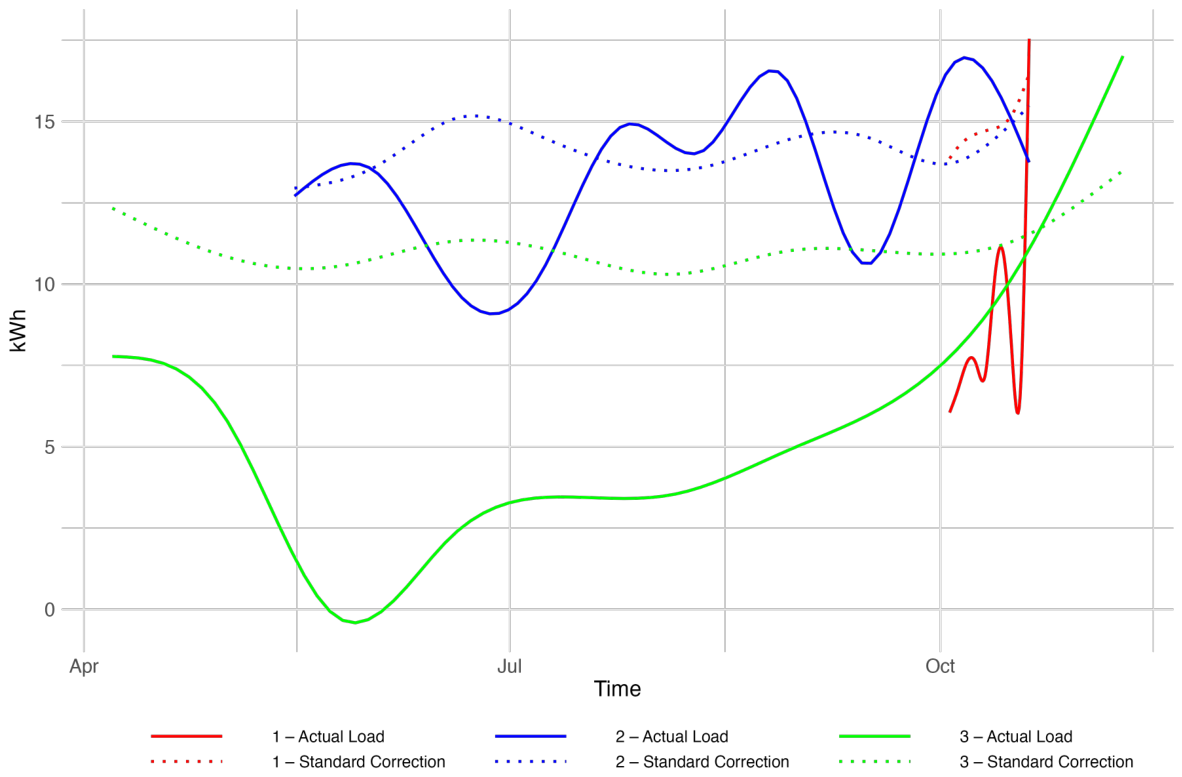
• Standard correction: The current standard correction data, acquired through MFFBAS, represents the net average electricity consumed per cable type for each quarter of an hour and each grid area [42]. This metric functions as an estimation of actual electricity load and is used by grid operators as a correction factor to determine the presence and extent of grid loss. The standard correction serves as a foundational comparison point for more nuanced analyses and will be used as a benchmark for assessing the predictive accuracy of the models. However, primarily because grid operators have not fully recognized their significance and due to the challenges in collecting all the necessary datasets, it does not account for various external factors that significantly influence load patterns. This might be the reason why the standard correction deviates so much from the real electricity load as illustrated in Figure 1. (The curves have been smoothed to highlight general load trends and systematic deviations between the actual and predicted values). Consequently, the research will explore the impact of including these additional variables in the models on the accuracy of the forecasts. (A detailed elaboration on how the standard correction is composed can be found in Appendix B.1).
• Weather variables: Data from the Koninklijk Nederlands Meteorologisch Instituut [43] is used, comprising measurements from 46 weather stations across the Netherlands. (It is acknowledged that weather data for the exact locations of the electrical substations are unavailable, so data from the nearest weather stations are used for the analysis). From this dataset, the variables $temperatur{e}_{it}$ and $sunshin{e}_{it}$ are extracted, where $temperatur{e}_{it}$ is linearly interpolated for quarter-hour intervals, while $sunshin{e}_{it}$ is evenly distributed across the hour. To capture the nonlinear relationship between temperature and electricity load, two variables are constructed: $pos\text{\_}{temp}_{it}$ (additional electricity required for cooling) and $neg\text{\_}tem{p}_{it}$ (increased electricity demand for heating), using a benchmark temperature of 20 degrees Celsius, which is widely used as a standard in building and environmental comfort studies. These are calculated as follows:

  $$pos\text{\_}tem{p}_{it}=\max (0,{\mathrm{temperature}}_{it}-20),$$

  (13)

  $$neg\text{\_}tem{p}_{it}=\max (0,20-{\mathrm{temperature}}_{it}),$$

  (14)
• Temporal factors: Indicator variables are used to include information on the time of day, day of the week, nighttime, weekends, public holidays, and whether the sun has risen. For public holidays, only the quarter-hours between 08:00 a.m. and 06:00 p.m. are used, as this is the period during which most people normally are working or at school but now have a day off and spend time at home. (The holidays considered can be found in Appendix B.2). Additionally, sunrise and sunset times are based on data from Amersfoort, often referred to as the geographical center of the Netherlands, making it a suitable proxy for the substations’ locations.
• Seasonal patterns: Seasonal patterns are modeled using lagged variables to capture periodic fluctuations in electricity load and reduce autocorrelation in the data. Each model is trained with and without the inclusion of four lagged variables of the dependent variable: $real\text{\_}load\text{\_}lag{1}_{it}$, $real\text{\_}load\text{\_}lag{2}_{it}$, $real\text{\_}load\text{\_}lag{96}_{it}$, and $real\text{\_}load\text{\_}lag{672}_{it}$, representing load one and two quarter-hours, one day, and one week prior, respectively. This approach assesses the significance of these variables and their impact on the models’ predictive performance.

Table 4. Description of the dependent and independent variables.

Variable	Description	Source
real_load	Electricity load in kWh per 15 min for each electrical substation	Enexis
standard_correction_ES	Average electricity consumed per cable type, per quarter of an hour, per grid area	MFFBAS
weekend	Indicator for weekends (1 if weekend, 0 otherwise)	Derived
night_time	Indicator for night time (1 between 01:00 and 07:00 a.m.)	Derived
work_hours	Indicator for work hours (1 during 09:00 a.m.–05:00 p.m., Mon–Fri)	Derived
evening	Indicator for evening hours (1 during 04:00 p.m.–10:00 p.m.)	Derived
holiday	Indicator for public holidays (1 during specific holidays)	Derived
sun_up	Indicator for daylight hours (1 from sunrise to sunset)	KNMI
sunshine	Duration of sunshine in minutes per quarter-hour	KNMI
pos_temp	Degrees Celsius above comfortable indoor temperature (20 °C)	KNMI
neg_temp	Absolute degrees Celsius below comfortable indoor temperature (20 °C)	KNMI
real_load_lag1	Lagged electricity load (one quarter of an hour prior)	Enexis
real_load_lag2	Lagged electricity load (two quarters of an hour prior)	Enexis
real_load_lag96	Lagged electricity load (one day prior)	Enexis
real_load_lag672	Lagged electricity load (one week prior)	Enexis

provides a concise description of the dependent and independent variables.

4.2. Data Preparation

To ensure robust and generalizable forecasting, the datasets are consolidated and prepared using the following steps:

• Stratified sampling and data allocation: Training, validation, and test sets are constructed using stratified sampling to ensure proportional representation from each segmented time period, maintaining overall dataset diversity. For the machine learning models, 70 percent of the data is allocated for training. The training set serves as the primary source for fitting the models, allowing them to learn the underlying patterns and relationships within the data. Subsequently, 15 percent is reserved for validation, aiding in hyperparameter tuning and model selection, while the remaining 15 percent is reserved for testing. In this setup, the test set serves as a novel dataset to evaluate the models’ ability to generalize, ensuring an impartial and objective assessment of their predictive performance.
• Feature alignment and standardization: All non-binary explanatory variables are aligned and standardized across all segments. Standardization involves scaling features to have zero mean and unit variance, ensuring consistency and comparability across different time periods and substations. This is crucial for the proper functioning of machine learning models, particularly those sensitive to feature scaling.

The process of data preparation and feature engineering is essential for creating a robust foundation for the predictive models. Stratified sampling ensures that each data subset used for training, validation, and testing accurately represents the variety of conditions observed in the full dataset. This approach enhances the generalizability of the models, making them more reliable in predicting electricity load across different substations and time periods.

5. Results

The forecasting accuracy and computational efficiency of all models are evaluated to identify those best-suited for practical application.

Table 5. Comparison of the utilized forecasting models.

Model	Variant	Overfitting	MAE	RMSE	MAPE
OLS	Regular	No	5.38	6.92 *	58.07
OLS	Lagged	No	1.64 *	2.39 **	24.91
ARIMAX	Regular	Yes	5.94	7.21 *	59.26
ARIMAX	Lagged	Yes	3.30	4.49 **	40.19
SARIMAX	Regular	Yes	5.67	6.92 *	55.34
SARIMAX	Lagged	Yes	4.39	5.47 **	47.05
Prophet	Regular	Yes	8.93	11.80	95.70
Prophet	Lagged	No	7.83	10.19 *	109.54
Decision Trees	Regular	Yes	5.74	7.74 *	68.99
Decision Trees	Lagged	No	2.57 *	3.60 **	41.34
Random Forests	Regular	Yes	5.01	6.92*	63.30
Random Forests	Lagged	No	1.66 *	2.50 **	24.71
Bagging Regression	Regular	Yes	5.15	7.14 *	64.06
Bagging Regression	Lagged	No	1.67 *	2.52 **	26.97
GBM	Regular	Yes	4.83	6.65 *	61.72
GBM	Lagged	Yes	1.64 *	2.45 **	24.96
XGBoost	Regular	Yes	4.99	6.58 *	53.85
XGBoost	Lagged	No	1.62 *	2.42 **	25.60
FNN	Regular	Yes	5.15	7.01 *	65.92
FNN	Lagged	No	1.66 *	2.48 **	23.68
SVR	Regular	Yes	4.96	6.55 *	56.66
SVR	Lagged	Yes	1.96 *	2.76 **	26.58
kNN	Regular	Yes	4.82	6.55 *	61.36
kNN	Lagged	Yes	2.13 *	3.00 **	26.47
Hybrid (approach A)	-	No	1.62 *	2.39 **	25.62
Hybrid (approach B)	-	No	1.61 *	2.38 **	23.97

Note: MAE and RMSE values are in kilowatt-hour (kWh), and MAPE values are presented in percentages. Moreover, an asterisk (*) denotes good performance, while two asterisks (**) indicate excellent performance.

presents the performance metrics and overfitting diagnostics for each model.

High MAPE values may result from data volatility, anomalies, or model-specific limitations. Despite this, the lowest MAPE remains a critical criterion for evaluating relative proportional prediction accuracy. Additionally, a detailed overview of computation times is provided in Appendix E.3. Most models, except for SARIMAX variants, complete fitting in less than 12 min. Predictions, except for Prophet and non-lagged SARIMAX models, are completed in under 5 s. Considering computational efficiency, performance metrics, and overfitting diagnostics, the top five individual models are: OLS with lagged variables, Random Forests with lagged variables, Bagging Regression with lagged variables, XGBoost with lagged variables, and Feedforward Neural Networks (FNN) with lagged variables. These models exhibit a balance between good to excellent performance in MAE and RMSE, reduced overfitting risks, and enhanced computational efficiency, making them highly practical for real-world applications.

Building on the previous evaluation, the top five models are compared in terms of statistically significant differences in predictive performance.

Table 6. Diebold–Mariano test results for pairwise model comparison.

Model Comparison	OLS	RF	BR	XGBoost	FNN
OLS	-	Significantly Better	Significantly Better	No Difference	Significantly Better
RF	Significantly Worse	-	No Difference	Significantly Worse	No Difference
BR	Significantly Worse	No Difference	-	Significantly Worse	No Difference
XGBoost	No Difference	Significantly Better	Significantly Better	-	Significantly Better
FNN	Significantly Worse	No Difference	No Difference	Significantly Worse	-

Note: “Significantly Better” indicates the model in the left column performs significantly better than the model in the top row; “Worse” indicates the opposite. “No Difference” indicates no significant difference in predictive accuracy.

presents the results of the Diebold–Mariano tests applied to each pair of these models.

The Diebold–Mariano test results reveal several noteworthy findings. First, OLS and XGBoost perform statistically on par with one another, and both significantly outperform RF, BR, and FNN. Second, RF, BR, and FNN show no significant differences among each other. Since these three models are statistically indistinguishable, computational efficiency is used as an additional criterion to select a third model alongside OLS and XGBoost: FNN has by far the shortest fitting time of the three (see Appendix E.3), and is therefore chosen. Based on the overall pairwise comparisons and this additional criterion, the three best-performing individual models are: OLS with lagged variables, XGBoost with lagged variables, and Feedforward Neural Networks (FNN) with lagged variables.

As shown in Table 5, both hybrid approaches do not exhibit overfitting and perform very similarly to one another. Hybrid approach B, which combines the predictions of the three base models through simple averaging, achieves the lowest MAE and RMSE of all evaluated models, while hybrid approach A, based on a stacked ensemble model, trails slightly behind on all three metrics. Both approaches slightly improve on the accuracy of their individual base models, indicating that combining these three models adds some value, although the improvement is modest. These results suggest strong absolute accuracy, although the relatively high MAPE highlights persistent challenges in capturing proportional accuracy. Furthermore, both hybrid models are highly computationally efficient, with fitting times of little over a minute and prediction times well under one second.

A direct comparison between the hybrid approaches and the top three individual models shows a mixed picture at the level of point estimates: hybrid approach B outperforms OLS and XGBoost on all three metrics (MAE, RMSE, and MAPE), though not FNN on MAPE, while hybrid approach A trails OLS on RMSE and MAPE and trails XGBoost on MAE. To assess whether these differences are statistically meaningful, the Diebold–Mariano test was conducted comparing both hybrid approaches with each of the top-performing individual models (OLS, XGBoost, and FNN). The results showed no significant difference between either hybrid approach and the OLS model. However, both hybrid approaches significantly outperformed the XGBoost and FNN models. A direct comparison between the two hybrid approaches themselves also showed no significant difference in predictive accuracy.

Following a comprehensive evaluation of all models, hybrid approach B is selected as the best-performing model for electricity load forecasting. Although hybrid approaches A and B are statistically indistinguishable in predictive accuracy, approach B is preferred for its structural simplicity: it does not require a separate meta-model, and consequently allows its base models to be trained on the full combined training and validation set, making more efficient use of the available data. Its predictive accuracy, on par with hybrid approach A and significantly better than XGBoost and FNN, allows it to closely track actual consumption values even under volatile conditions—an essential feature for operational and planning purposes in electricity management. Notably, while OLS with lagged variables performs statistically on par with both hybrid approaches, hybrid approach B achieves marginally better point estimates than OLS across MAE, RMSE, and MAPE, suggesting that combining multiple models can still yield a modest edge over the simpler linear alternative.

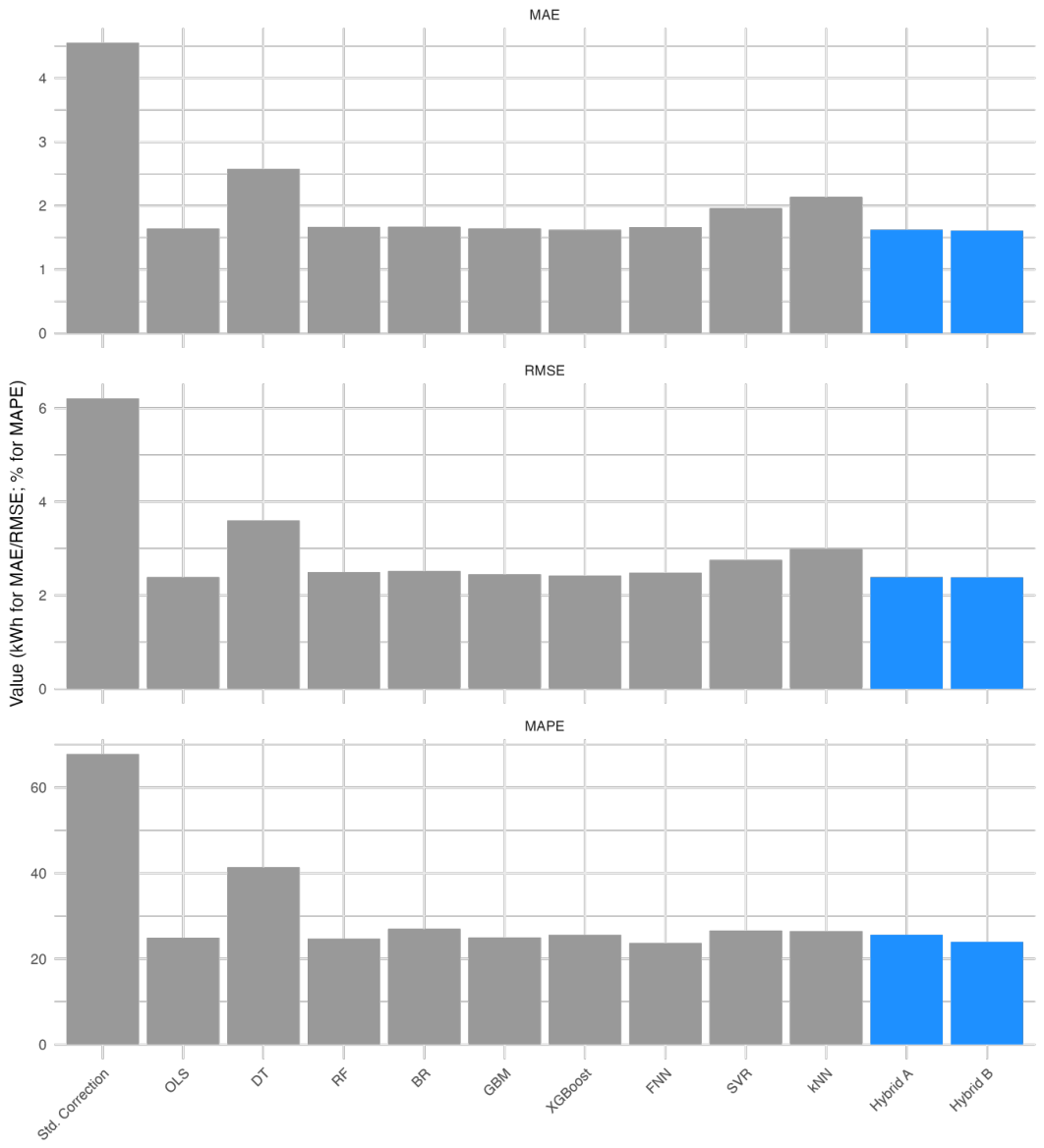
Compared to the standard correction currently used by grid operators, hybrid approach B performs significantly better. The standard correction yields a MAE of 4.55, RMSE of 6.21, and MAPE of 67.82, which are substantially worse than the top-performing model. Specifically, relative to the standard correction, hybrid approach B reduces MAE by 2.94 kWh, corresponding to a 64.7% reduction in the average deviation between predicted and actual load. A paired t-test confirms that the improvements achieved by hybrid approach B are statistically significant, with a p-value well below 0.05. These findings underscore the value of advanced techniques and the inclusion of additional predictors in improving electricity load forecasts beyond traditional methods. Figure 2 presents these results in a comparative visualization across all lagged individual models, both hybrid approaches, and the standard correction method, confirming that the standard correction’s error is substantially higher than that of any individual or hybrid model across all three metrics.

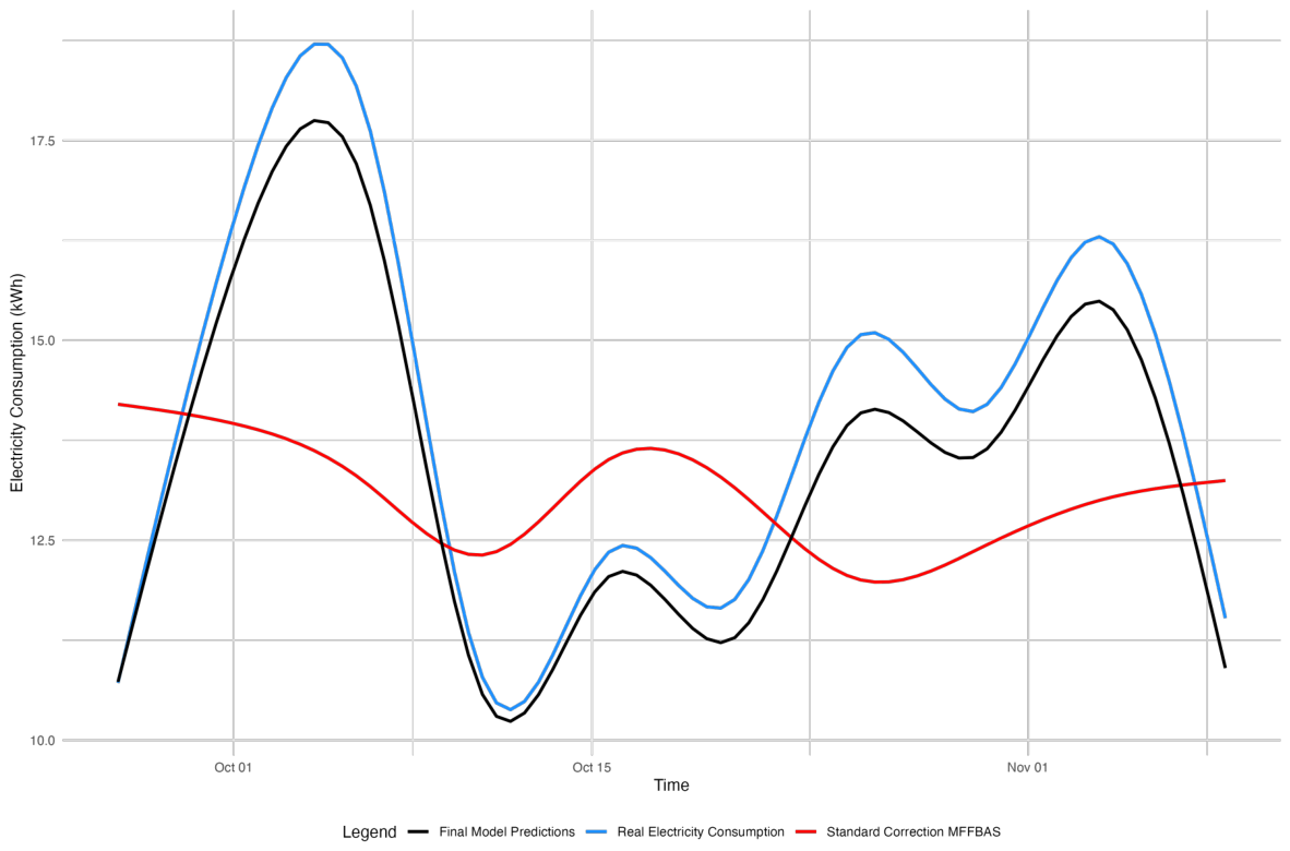
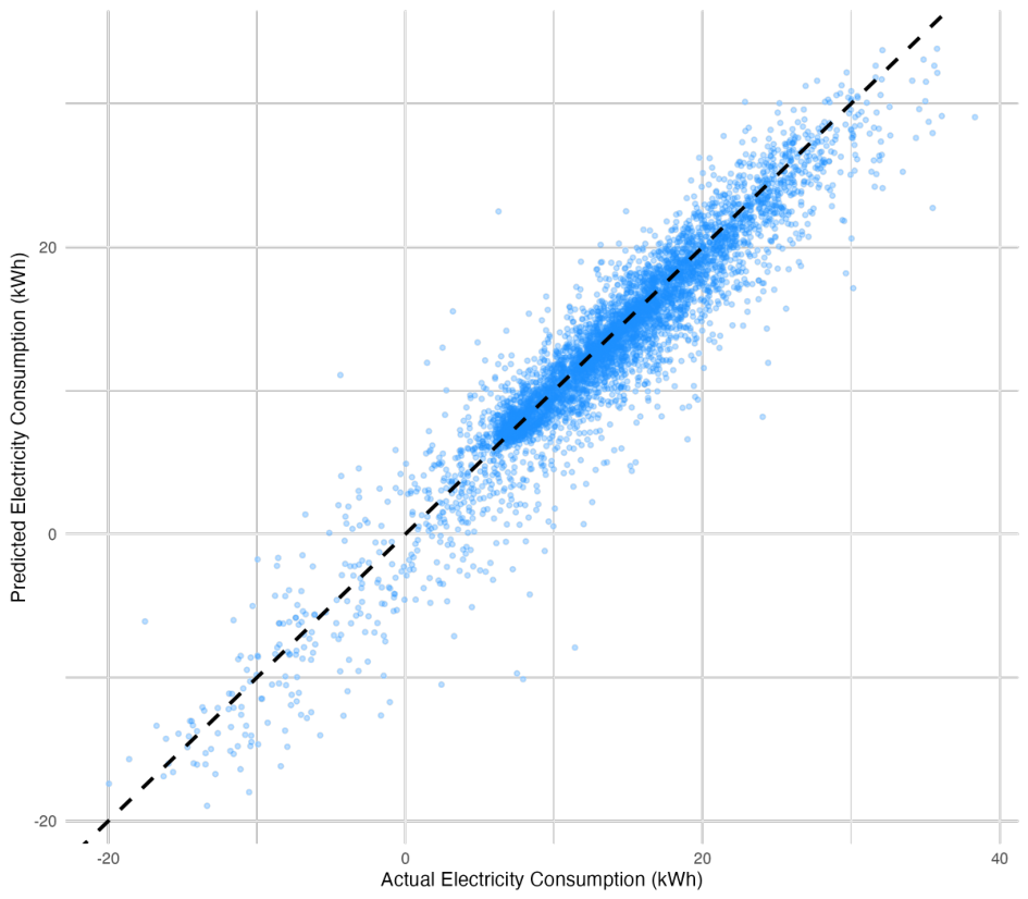
Figure 3 illustrates this improvement visually, showing that hybrid approach B’s predictions closely track the volatile fluctuations in actual consumption, whereas the standard correction remains comparatively flat and fails to capture these short-term dynamics. To further validate the predictive accuracy of hybrid approach B, Figure 4 plots predicted against actual electricity consumption on the test set: the tight clustering around the diagonal reference line confirms strong agreement between predictions and observed values, with deviations concentrated among a small number of extreme observations. 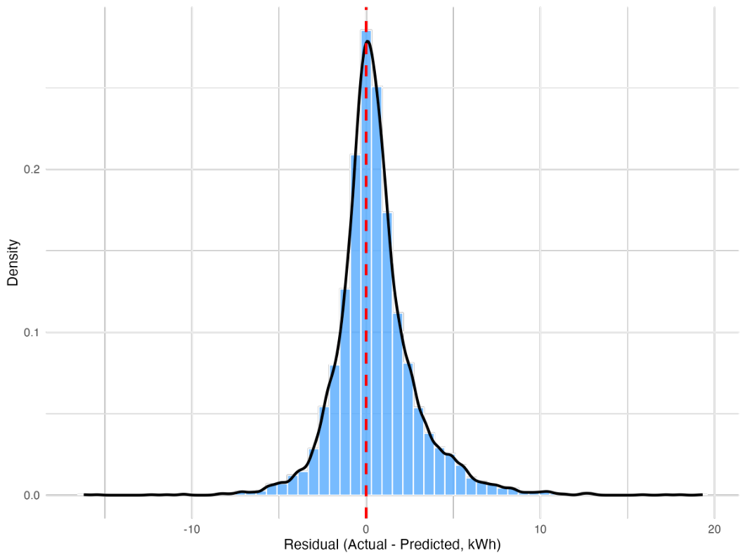Figure 5 shows the corresponding distribution of residuals, which is unimodal, approximately symmetric, and centered close to zero, indicating no systematic bias in the model’s predictions.

To interpret the performance of the hybrid averaging model, it is useful to consider the complementary characteristics of its constituent forecasting methods. OLS captures the dominant linear relationships between the lagged consumption values and the other predictors, providing a stable, low-variance baseline. XGBoost captures nonlinear interactions and localized patterns through sequential tree-based boosting, which a purely linear model cannot represent. Feedforward Neural Networks are well-suited to learning smooth, continuous functional relationships that tree-based models may approximate more coarsely. Because these models rely on different functional forms, their forecast errors are not identical, although they remain fairly strongly correlated, as all three are exposed to the same underlying signal and noise in electricity consumption. (Pairwise Pearson correlations between the models’ forecast errors on the test set range from 0.92 to 0.94). Averaging their predictions therefore only modestly reduces model-specific biases and variance, which provides a plausible explanation for the hybrid model’s consistent, if modest, improvement relative to the individual models.

6. Discussion

The results show a clear improvement in forecasting accuracy once lagged variables are included, indicating that short-run persistence in substation load is a major driver of predictive performance. This is consistent with the idea that electricity demand at the substation level is strongly shaped by very recent consumption patterns, alongside daily and weekly cycles. In practical terms, the lagged variables appear to capture the immediate structure of the load series better than models relying only on weather and calendar information.

Among the hybrid approaches, the simple averaging model and the stacked ensemble performed statistically indistinguishably from one another. This is plausible given that the three base models—OLS, XGBoost, and FNN—capture different aspects of the data but nonetheless produce fairly correlated forecast errors, limiting the extent to which either combination strategy can meaningfully outperform the other. The stacked ensemble is, in principle, more susceptible to the limited amount of validation data available for fitting the meta-learner, which introduces additional estimation noise not present in the simple averaging approach; this may explain the preference for averaging in practice, despite the two approaches performing comparably overall. These results suggest that, for discontinuous substation-level load data, a simpler hybrid strategy is at least as effective as a more complex stacking procedure, while being structurally more robust.

The fact that the advanced models outperform the standard correction suggests that the current correction-based approach used by grid operators leaves relevant information unused. In particular, the standard correction does not fully incorporate location-specific temporal structure, weather sensitivity, or recent load history, all of which matter in short-horizon forecasting. The strong performance of models that do include these variables supports the view that more granular and data-driven forecasting can improve operational decision-making in distribution networks. This also aligns with prior forecasting research showing that lagged load values and exogenous variables often improve predictive accuracy in electricity demand applications.

These findings are important for grid-loss detection because the forecasting model is not an end in itself, but a tool for improving the signal used to identify abnormal deviations. A more accurate expected-load estimate makes it easier to distinguish normal consumption variation from losses caused by electricity theft, defective meters, or cable faults. In that sense, the main value of the proposed approach lies in improving the reliability of the benchmark against which grid losses are detected, rather than merely producing lower forecasting errors. In practical terms, this could be integrated into the grid operator’s monitoring workflow by flagging unusually large deviations between predicted and observed load for further inspection. Because load patterns may change over time, periodic retraining and ongoing performance monitoring would also be necessary to address concept drift and preserve model reliability.

Several limitations should be kept in mind. The dataset does not include winter months, so the models may not fully capture colder-season consumption behavior or seasonal extremes. The analysis also lacks electricity price variables, while consumer behavior—particularly among users with variable contracts—may shift in response to price changes. Additionally, socio-economic characteristics (e.g., building types, income levels, population density) and local infrastructure elements (e.g., solar panels, street lighting, and EV charging stations) were not included, all of which may help explain some of the remaining variation in load. The weather variables are also treated linearly due to the available data’s granularity, which may oversimplify the actual, potentially nonlinear, relationship between weather conditions and electricity consumption. Future work could address these issues by using a longer time span and richer covariates.

Moreover, while the computational results indicate that the proposed forecasting pipeline is compatible with short-horizon operational use, a full analysis of real-time deployment, integration with existing grid monitoring systems, and large-scale scalability across many substations lies beyond the scope of this study and remains an important direction for future work.

Finally, the discontinuous panel structure of the data remains an important methodological constraint. Although the results suggest that the models generalize reasonably well across segmented substation periods, the absence of a fully continuous time series means that caution is still needed when extrapolating to other substations or longer forecasting horizons. Even so, the findings indicate that substation-level forecasting can provide a practical and scalable improvement over the current correction-based approach, especially for strengthening grid-loss detection rather than forecasting demand for its own sake.

Based on these potential improvements, several directions for future research are recommended. First, incorporating dynamic electricity prices could improve the model’s responsiveness to behavioral patterns. Second, expanding standard corrections to include all cable types would allow for more accurate baseline estimations. Third, using nonlinear modeling techniques—particularly for weather-related variables—may better capture complex interactions. Moreover, including winter data and seasonal dummy variables could help eliminate seasonal bias. Lastly, enriching the dataset with socio-economic and infrastructure-related variables, and expanding its scope across more substations and longer timeframes, would enhance the model’s robustness, applicability, and potential for real-time grid management support.

7. Conclusions

Grid losses impose substantial financial and operational burdens on grid operators, particularly in the context of rising energy prices and electricity theft. Improving the accuracy of substation-level electricity load forecasting can support early detection of these losses and contribute to more efficient grid management. This study examined whether the standard correction method currently used by Dutch grid operators could be improved through advanced forecasting techniques. A wide range of statistical and machine learning models was applied to detailed quarter-hourly electricity load data, along with a set of exogenous variables not currently used in practice.

The results show that several individual models, particularly those incorporating lagged variables, outperformed the standard correction method. Among the two hybrid approaches—both combining the predictions of the best-performing individual models, OLS, XGBoost, and FNN—the simple averaging approach was selected as the overall best model. Its predictive accuracy was statistically indistinguishable from both the stacked ensemble approach and OLS individually, and significantly better than XGBoost and FNN individually, confirmed by the Diebold–Mariano test. The averaging approach was preferred over the stacked ensemble for its structural simplicity, as it does not require a separate meta-model and can therefore use the full training and validation data for its base models. It was preferred over OLS for its marginally better point estimates across all three metrics, and because averaging multiple, structurally different models generally improves robustness compared to relying on a single model.

Despite the clear improvements in forecasting accuracy in the proposed models, a number of avenues for further improvement remain. By including data from winter months, the model’s seasonal generalizability may be improved. Additionally, key predictors such as electricity prices, socio-economic indicators, and local infrastructure characteristics were not included. Incorporating such variables in future research may lead to further improvements in forecasting performance. Overall, the findings demonstrate that data-driven forecasting approaches can substantially improve substation-level load prediction, providing a strong foundation for more effective grid loss detection.

Ultimately, while the forecasting models developed in this study do not reduce grid loss directly, their value lies in strengthening the operational detection mechanisms used by grid operators. More accurate and temporally precise load forecasts allow deviations from expected consumption to be identified earlier and more reliably, enabling faster and more targeted interventions against electricity theft, defective meters, or cable faults. As a result, the improved forecasting accuracy demonstrated in this study provides a concrete pathway toward reducing energy losses in real-world grid operations.