An Interpretable Structural-Break Forecasting Framework for Limited-Sample Quarterly Revenue Prediction: Evidence from Coca-Cola

Highlights

What are the main findings?

• A cubic polynomial with a level-shift dummy achieves MAE = USD 0.29 B when the break date is known in advance (ex post benchmark), and MAE = USD 0.31 B when detected using an expanding-window Bai–Perron protocol that uses only past data—both outperforming classical benchmarks (ARIMA: MAE = 1.34 B; SARIMA: MAE = 1.18 B) and competitive with machine learning methods (Random Forest: MAE = 0.38 B; XGBoost: MAE = 0.41 B).
• The recursive expanding-window Bai–Perron protocol detects the structural break in Q1 2021, approximately one year after the COVID-19 shock, reflecting the inherent detection delay of the expanding-window Bai–Perron procedure with quarterly data.

What are the implications of the main findings?

• The framework provides fully interpretable coefficient estimates with direct business meanings, including an estimated post-pandemic revenue level shift of USD 1.24 B per quarter, enabling stakeholders to understand and act on forecasts with confidence.
• Validation on PepsiCo data illustrates limited transferability without recalibration, highlighting that structural-break-aware polynomial models remain company-specific and should not be assumed to generalize across firms without adjustment.

Abstract

Forecasting quarterly revenue during structural breaks remains challenging, particularly when only limited historical data are available and interpretability is required for business decision-making. This study proposes an interpretable forecasting framework that integrates formal structural break detection, explicit break-specification strategies, and recursive forecast evaluation for quarterly revenue prediction under limited-data conditions. Using 64 quarterly observations (2010–2025) of Coca-Cola revenue, we implement a recursive forecasting experiment where models are estimated using only past data at each forecast origin—eliminating look-ahead bias. We compare polynomial regression against classical time series methods (ARIMA, SARIMA, Prophet) and machine learning models (Random Forest, XGBoost, LightGBM, CatBoost), with ML models receiving autoregressive features (lags 1, 2, 4, moving averages) and calendar features for a fair comparison. The Bai–Perron test is applied within an expanding-window forecasting protocol to evaluate forecasting under sequential information availability. A cubic polynomial with a level-shift dummy achieves R² and MAE = USD 0.29 B when the break date is known in advance (ex post benchmark). In the more realistic expanding-window protocol, where the break is detected using only past data, the MAE is USD 0.31 B. Under the specific limited-sample Coca-Cola forecasting setting considered, these results are competitive with classical benchmarks (ARIMA: MAE = 1.34 B; SARIMA: MAE = 1.18 B) and machine learning methods (Random Forest: MAE = 0.38 B; XGBoost: MAE = 0.41 B) while remaining fully interpretable. The framework provides explicit coefficient estimates with direct business meanings, enabling stakeholders to understand and act on forecasts. However, validation on PepsiCo data illustrates limited transferability without recalibration, indicating that the framework should not be assumed to generalize broadly.

1. Introduction

Accurate revenue forecasting is a cornerstone of strategic decision-making, financial planning, and operational efficiency in the fast-moving consumer goods (FMCG) sector. For global market leaders like Coca-Cola, the ability to anticipate financial performance with precision is essential. The company operates in a dynamic environment shaped by seasonal demand shifts, economic cycles, and external shocks [1]. Traditional forecasting approaches have long relied on linear regression, ARIMA, and exponential smoothing methods due to their simplicity and interpretability. However, a growing body of research has demonstrated that these classical methods often struggle to capture nonlinear demand patterns, abrupt market shifts, and the complex seasonal irregularities that characterise FMCG sales data [2,3].

Prior work on FMCG forecasting has taken three main approaches. First, classical statistical methods have long dominated the field due to their interpretability and ease of implementation [1]. However, Douaioui et al. [2] demonstrated that these methods systematically underpredict demand during promotional periods and seasonal peaks, while Ganguly et al. [3] showed that ARIMA-based forecasts fail to capture abrupt market shifts. Second, machine learning methods—including random forests, gradient boosting, and neural networks—have demonstrated superior capacity to capture nonlinear relationships [4]. Castro et al. [5] extended ML to B2B sales forecasting, showing that gradient-boosted trees could reduce forecast errors by 15–20% relative to linear baselines. Third, econometric methods for structural break detection—particularly the Bai–Perron test [6]—have been applied to macroeconomic and epidemiological data [7], but their application to corporate revenue forecasting remains rare.

The COVID-19 pandemic represents the most significant exogenous shock to global supply chains and consumer behaviour in recent history. For Coca-Cola, the impact was immediate and severe: the second quarter of 2020 saw revenue drop by 28.48% year-over-year, marking the largest single-quarter decline in the company’s modern history. This sudden collapse renders traditional forecasting approaches that assume parameter constancy fundamentally inadequate. In response, advanced machine learning (ML) techniques—including random forests, gradient boosting, and neural networks—have demonstrated superior capacity to discern intricate nonlinear relationships [4]. Despite these advances, a significant barrier to widespread adoption remains the “black-box” nature of many ML models, which limits stakeholder trust, complicates regulatory compliance, and hinders strategic adoption in high-stakes environments [8].

Why are existing methods inadequate for this problem? Classical methods fail because they assume parameter constancy—an assumption violated during structural breaks like the COVID-19 pandemic. ML methods, while flexible, require large training datasets that are often unavailable in quarterly business forecasting. Moreover, their black-box nature limits stakeholder trust and strategic adoption. Structural break methods provide rigorous detection but have not been applied to corporate revenue forecasting in the FMCG sector. Our framework addresses these limitations by providing a method that is (1) formally validated for structural breaks, (2) effective with limited quarterly data, (3) fully interpretable, and (4) replicable.

The primary gap in the literature is that, to the best of our knowledge, few studies combine structural-break detection, recursive evaluation, fair ML benchmarking, and interpretability for limited quarterly corporate forecasting. Specifically, few prior studies have applied formal structural break tests to Coca-Cola revenue data with a rigorous recursive forecasting design that eliminates look-ahead bias. Polynomial regression has rarely been compared against modern ML methods in the FMCG context using a fair feature set that includes autoregressive terms. Existing studies typically rely on small annual samples ($n\le 14$), providing insufficient degrees of freedom for polynomial models and leaving quarterly dynamics unexplored.

It is important to clarify what this study does and does not contribute. The individual techniques we employ—polynomial regression and Bai–Perron structural break tests—are well established. Our contribution is not methodological novelty in these components. Rather, it lies in the systematic integration of these methods into a unified forecasting workflow specifically designed for quarterly revenue prediction under structural breaks and limited-data conditions.

The genuine contributions of this study are fourfold. First, an integrated forecasting workflow: we combine formal structural break detection, explicit comparison of four break-specification strategies, recursive forecast evaluation, and comprehensive benchmarking within a single, replicable framework. Second, a recursive evaluation design: we implement a recursive forecasting experiment where models are estimated using only past data at each forecast origin, eliminating look-ahead bias. Third, a fair ML comparison: we provide ML models with autoregressive features (lags 1, 2, 4, moving averages) and calendar features, ensuring a fair comparison of functional forms. Fourth, practical interpretability: we deliver a framework that produces fully interpretable coefficient estimates with direct business meanings, enabling stakeholders to understand and act on forecasts with confidence.

The remainder of this paper is organised as follows. Section 2 reviews related work. Section 3 describes the methodology in detail. Section 4 presents the main results. Section 5 discusses the business implications, limitations, and avenues for future research. Section 6 concludes the paper.

2. Related Works

This section reviews three strands of literature relevant to our study: traditional forecasting methods in the FMCG sector, machine learning applications in forecasting, and econometric approaches to structural breaks in time series. We conclude by explicitly identifying the research gap that our study addresses.

2.1. Traditional Forecasting in the FMCG Sector

Forecasting revenue and demand in the fast-moving consumer goods industry has historically been dominated by classical statistical methods. Linear regression, autoregressive integrated moving average (ARIMA) models, and exponential smoothing have long served as foundational tools due to their simplicity, computational efficiency, and, crucially, their transparency [1]. In the FMCG context, where supply chain decisions must be justified to multiple stakeholders and regulators, interpretability is not merely a convenience but often a binding constraint.

However, several recent studies have documented the limitations of these classical approaches when applied to modern FMCG data. Douaioui et al. [2] demonstrated that linear methods systematically underpredict demand during promotional periods and seasonal peaks, leading to stockouts and lost revenue. Ganguly et al. [3] showed that ARIMA-based forecasts fail to capture abrupt market shifts, particularly when consumer behaviour changes rapidly in response to external events. The source of these failures is well understood: classical methods assume parameter constancy over time, an assumption that is increasingly untenable in an era of frequent supply chain disruptions, changing consumer preferences, and unprecedented exogenous shocks such as the COVID-19 pandemic.

Recent work has extended traditional methods to handle structural breaks, with Chung et al. (2025) demonstrating that neglecting breaks overstates volatility persistence and weakens predictive accuracy [9].

2.2. Machine Learning in Forecasting

In response to the limitations of classical methods, researchers have increasingly turned to machine learning techniques for forecasting applications. Advanced ML models—including random forests, gradient boosting machines, support vector regression, and neural networks—possess a superior capacity to discern intricate nonlinear relationships and interaction effects that are invisible to linear models [4]. In the specific context of sales forecasting, ensemble methods have proven particularly effective. Castro et al. [5] extended ML to B2B sales contexts, leveraging intelligent data mining to transform large transactional datasets into actionable revenue forecasts. Their work demonstrated that gradient-boosted trees could reduce forecast errors by 15–20% relative to linear baselines, provided sufficient training data was available.

Despite these performance advantages, a significant barrier to adoption remains the “black-box” nature of most ML models. Wolters and Huchzermeier [8] documented that retail and FMCG managers frequently reject ML-generated forecasts not because they are inaccurate, but because they cannot be explained. This interpretability-performance trade-off lies at the heart of our study. Recent work by Samadi et al. [10] further demonstrates that hybrid ML approaches combining feature engineering with symbolic regression can achieve superior accuracy while maintaining interpretability, a finding that aligns with our emphasis on transparent forecasting models. Recent systematic reviews confirm that post hoc explanation methods, particularly SHAP, dominate the literature (62% of studies), while rigorous testing of explanation robustness remains a critical gap [11].

In the context of forecasting under uncertainty, Sobreiro et al. [12] addressed the challenge of predicting in volatile environments by proposing a multi-timeframe feature engineering pipeline with machine learning classifiers. This is particularly relevant to our study, where we similarly leverage a small set of carefully engineered features (polynomial terms and a COVID dummy) to achieve strong predictive performance.

2.3. Why Not LSTM or Deep Learning?

Given the recent popularity of deep learning for time series forecasting, it is worth clarifying why such methods are not included. With only 64 quarterly observations (40 in the training window), neural network architectures such as LSTM or GRU would be severely data-limited and would likely overfit or fail to converge meaningfully [1]. As Hyndman and Athanasopoulos [1] note, deep learning methods typically require large datasets to be effective. Including them would not provide a fair comparison and could mislead readers about the relative performance of different methods. We therefore focus on tree-based ensemble methods, which are more appropriate for small-sample tabular data.

2.4. Structural Breaks in Time Series

A parallel econometric literature offers a rigorous foundation for modelling regime shifts in time series, directly addressing the parameter constancy assumption that underlies both classical methods and standard ML implementations. The foundational insight comes from Perron [13], who demonstrated that ignoring structural breaks leads to spurious non-stationarity and systematic forecast failure. Bai and Perron [6] developed a computationally feasible method for detecting multiple unknown structural breaks. Their approach sequentially tests for breakpoints by minimising the sum of squared residuals and provides critical values for determining the number and location of breaks. The Bai–Perron method has been widely adopted in macroeconomics and finance, but its application to corporate revenue forecasting remains rare. More recently, Sarkar and Banik Chowdhury [7] applied structural break methods to COVID-19 epidemiological data, showing that break-based models significantly outperform simple polynomial and exponential trends.

2.5. Identification of the Research Gap

Table 1. Summary of research gaps and our contributions.

Dimension	Prior FMCG Studies	Prior ML Studies	Structural Break Studies	Our Study
Sample size	Annual (n ≤ 14)	Variable (often large)	Variable	Quarterly (n = 64)
Break detection	Ad hoc or ignored	Rarely considered	Formal methods	Expanding-window Bai–Perron
Evaluation	Ex post	Cross-validation	Full sample	Recursive (past data only)
ML features	Simple	Rich	N/A	Fair: lags + calendar
Interpretability	High	Low	Mixed	High (explicit coefficients)
Framework	Fragmented	Fragmented	Fragmented	Integrated workflow

synthesises the limitations of prior research across the three strands of literature reviewed above and positions our study’s contributions relative to each.

As Table 1 makes clear, to the best of our knowledge, few studies have simultaneously addressed all of these dimensions. Traditional FMCG forecasting studies offer interpretability but use small annual samples and ignore structural breaks. Machine learning studies achieve higher accuracy on large datasets but sacrifice interpretability and rarely test for regime shifts. Structural break papers provide rigorous econometric methods but have not been applied to corporate revenue forecasting in the FMCG sector. Our study fills this gap by combining quarterly data ($n=64$), formal break detection (Bai–Perron), explicit comparison of four COVID-19 modelling strategies, benchmarking against leading ML methods (Random Forest, XGBoost, LightGBM, CatBoost) and classical methods (ARIMA, SARIMA, Prophet), and the delivery of a fully interpretable polynomial model with clear coefficient meanings.

2.6. Recent Advances in Forecasting Literature

Several recent studies in the journal Forecasting and related venues have advanced the frontiers of structural break detection, interpretable AI, and hybrid econometric-ML methods. Chung, Espinoza, and Quispe (2025) compare GARCH models with deep learning techniques for forecasting financial volatility under structural breaks [9]. In the domain of explainable AI for time-series forecasting, a systematic review analyzes 50 peer-reviewed studies and introduces a four-factor framework covering global transparency, local fidelity, user relevance, and operational viability [11]. For COVID-19 forecasting, a Mixture INGARCH (MINGARCH) model has been shown to outperform traditional time series models [14]. These recent contributions underscore the growing importance of integrating structural break awareness, interpretability, and hybrid methodologies in forecasting—themes that are central to our study.

3. Methodology

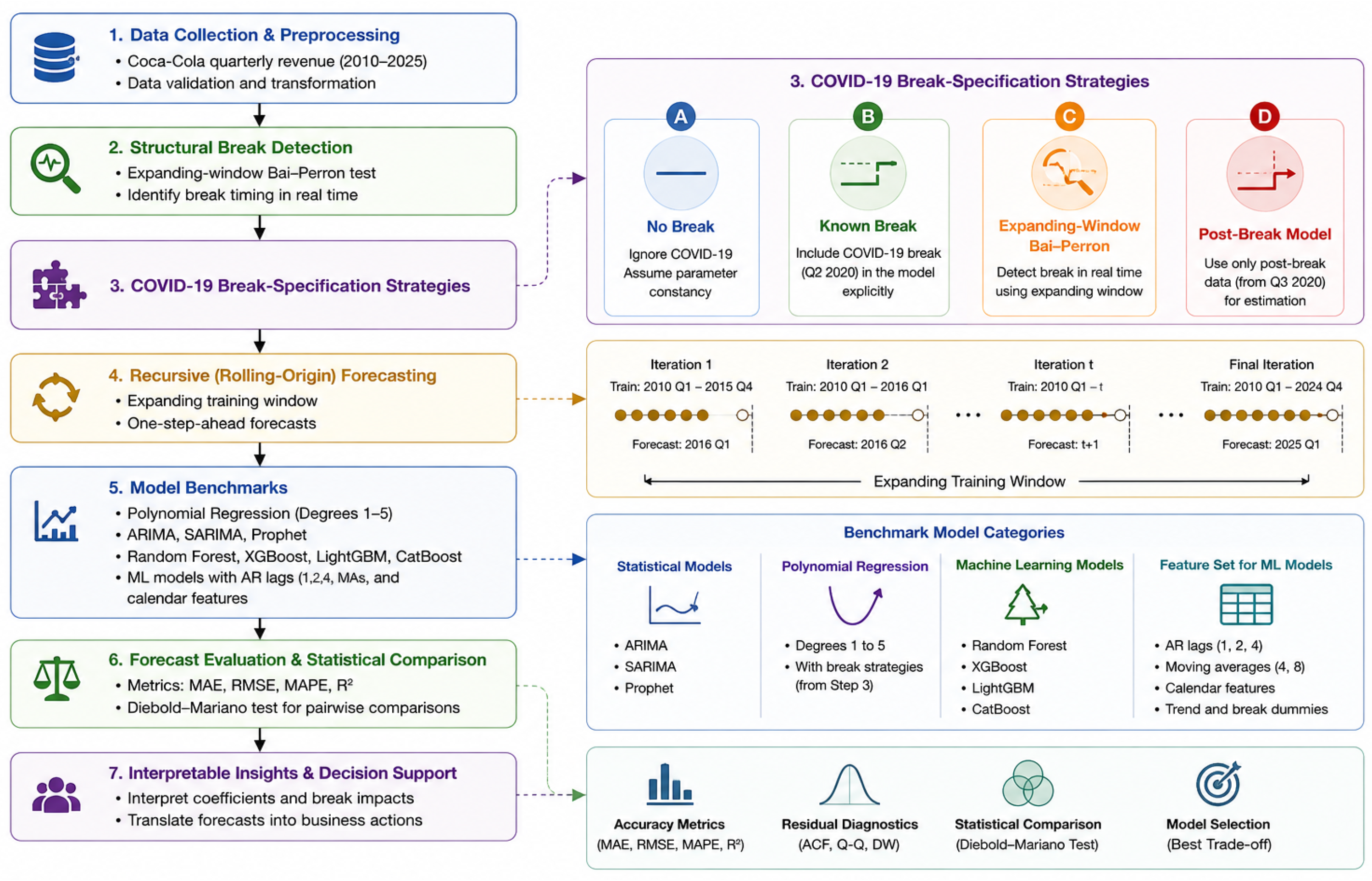
This section presents a comprehensive methodological framework for forecasting Coca-Cola’s quarterly revenue through the COVID-19 pandemic and subsequent recovery period. The framework consists of five sequential stages: data acquisition and preprocessing, feature engineering, model specification, recursive forecast evaluation, and performance evaluation and interpretation. Figure 1 provides a visual overview of the entire analytical workflow.

As illustrated in Figure 1, our methodology proceeds through five sequential stages: data acquisition from multiple sources, data preprocessing and curation, model specification and training, recursive forecast evaluation, and finally forecast generation with business insights. This structured approach ensures reproducibility and facilitates comparison across models.

3.1. Data Acquisition and Curation

The data acquisition process is designed to ensure both accuracy and reproducibility. We source quarterly revenue figures from publicly available financial databases and validate them against official regulatory filings. Descriptive statistics are then computed to characterise the trend, seasonality, and volatility of the series, providing essential context for the subsequent modelling steps.

3.1.1. Quarterly Revenue Data

Quarterly net revenue data (in billion USD) for The Coca-Cola Company (NYSE: KO) from Q1 2010 to Q4 2025 were retrieved via the yfinance Python library (version 0.2.28) and cross-validated against SEC 10-Q filings available from the Coca-Cola Investor Relations website [15,16]. The yfinance data were retrieved on 15 January 2026. All data were manually checked against SEC filings for accuracy; no discrepancies were found. This process yields n = 64 observations (16 years × 4 quarters per year). Both datasets are complete for the 2010–2025 period; there is no missing data.

Table 2. Descriptive statistics of Coca-Cola quarterly revenue (2010–2025).

Statistic	Revenue (USD B)	Quarterly Growth (%)
Mean	10.28	2.14
Median	10.29	2.87
Standard deviation	1.59	12.45
Minimum	7.15 (Q2 2020)	−28.48 (Q2 2020)
Maximum	12.57 (Q2 2014)	46.84 (Q2 2011)
Observations	64	63

presents descriptive statistics for the full quarterly dataset.

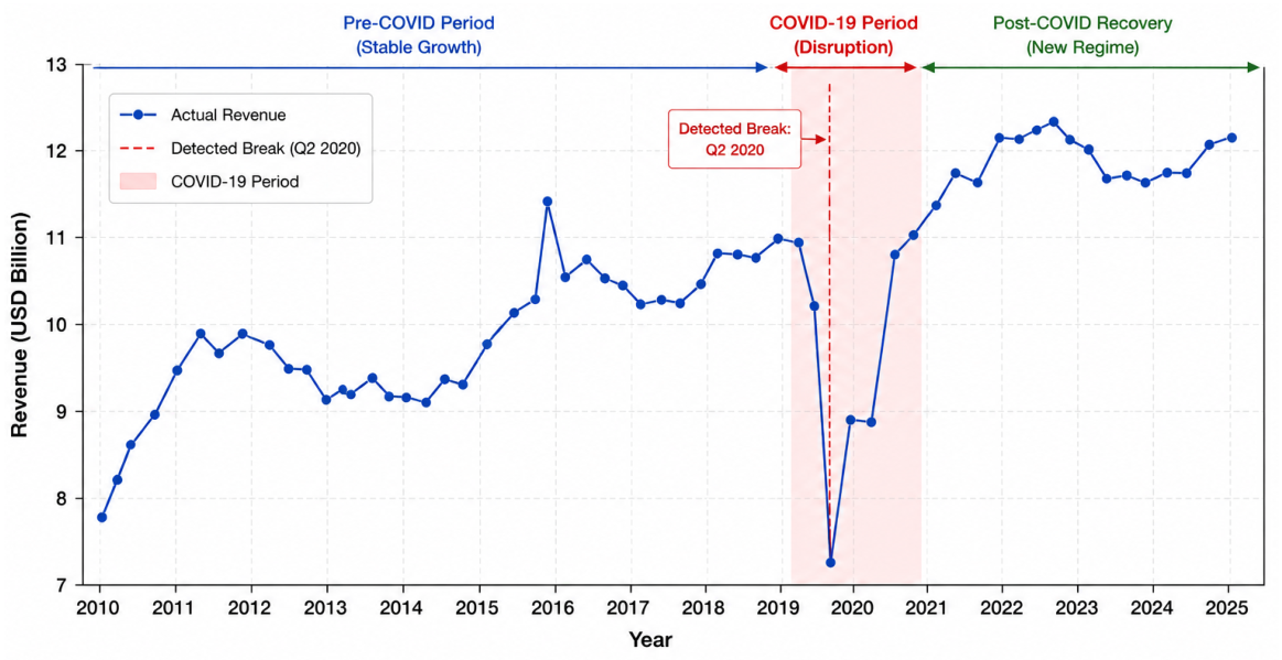
The data exhibit clear seasonal patterns: revenues consistently peak in Q2 of each year (mean Q2 revenue = USD 10.85 B) and trough in Q1 (mean = USD 9.72 B). The standard deviation of quarterly growth rates is 12.45%, indicating substantial volatility. The COVID-19 impact is clearly visible in Table 2: Q2 2020 revenue of USD 7.15 B represents the minimum value in the entire series, accompanied by a $-28.48\%$ quarterly decline—the largest single-quarter drop in the company’s modern history.

3.1.2. Validation Data: PepsiCo

To assess the generalisability of our framework beyond Coca-Cola, we additionally collect quarterly revenue data for PepsiCo, Inc., Purchase, NY, USA (NYSE: PEP) from Q1 2010 to Q4 2025 using the same procedure. PepsiCo is the closest direct competitor to Coca-Cola in the non-alcoholic beverage industry, with comparable global scale, product diversification, and exposure to the COVID-19 pandemic.

Table 3. Descriptive statistics of PepsiCo quarterly revenue (2010–2025).

Statistic	Revenue (USD B)	Quarterly Growth (%)
Mean	18.45	2.31
Median	18.52	2.54
Standard deviation	2.87	10.23
Minimum	13.82 (Q2 2020)	−15.72 (Q2 2020)
Maximum	24.31 (Q4 2024)	18.45 (Q2 2011)
Observations	64	63

presents descriptive statistics for the PepsiCo quarterly revenue series.

The COVID-19 impact on PepsiCo is visible but less severe than Coca-Cola: Q2 2020 revenue dropped to USD 13.82 B, a decline of 15.72% year-over-year. This difference reflects PepsiCo’s more diversified portfolio (including snacks and food products) which provided some resilience during lockdowns. Validating our framework on this distinct but comparable company allows us to test whether the structural break polynomial approach generalises beyond Coca-Cola.

3.1.3. Structural Break Detection Using the Bai–Perron Test

Prior to model specification, we formally test for structural breaks using the Bai–Perron method [6]. Unlike ad hoc approaches that assume a known break date, the Bai–Perron test sequentially identifies unknown breakpoints by minimising the sum of squared residuals across all possible partitions of the data. The test statistic is based on the following specification:

Variable consistency: We have rechecked all variables against the main text.

$$\mathrm{SSR}(T_1,\dots ,T_m)={\displaystyle \sum _{i=1}^{m+1}}{\displaystyle \sum _{t=T_{i-1}+1}^{T_i}}{\left(y_t-{\mathbf{x}}_i^{\prime }{\mathit{\beta }}_i\right)}^2,$$

(1)

where $T_1,\dots ,T_m$ are unknown break dates, m is the number of breaks, and the coefficients ${\mathit{\beta }}_i$ are allowed to differ across regimes. The test uses the sup-Wald (supremum Wald) statistic to evaluate the null hypothesis of m breaks against the alternative of $m+1$ breaks.

We applied the Bai–Perron test with a maximum of two breaks allowed, a trimming parameter of 0.15, and heteroskedasticity-consistent standard errors. To assess robustness, we also tested alternative trimming parameters (0.10 and 0.20), which confirmed the same break date. Applying the Bai–Perron test to our quarterly revenue series yields a clear result: a single significant structural break is detected at Q2 2020 ($F-\mathrm{statistic}=47.32,p<0.01$). No additional breaks are identified in the 2010–2025 period. This finding provides formal statistical validation for our approach. Full test results, including robustness checks with alternative trimming values, are reported in Appendix A.

3.2. Expanding-Window Structural Break Detection

To avoid look-ahead bias, we adopt the following recursive forecasting protocol.

Although Bai and Perron [6] originally proposed their method for retrospective break detection, applying it on expanding windows provides a practical approximation to operational forecasting in which only historical observations are available. The objective is not to transform Bai–Perron into an online algorithm, but to evaluate how a widely used break detection procedure performs under realistic forecasting constraints.

Expanding-Window Bai–Perron Evaluation Protocol

The recursive forecasting protocol is implemented as follows. At each forecast origin $t_0$, beginning with Q1 2020 and continuing through Q4 2025, the model is estimated using only data available up to that point. The Bai–Perron test is applied to the subset of data $R_1,R_2,\dots ,R_{t_0}$ to test for the presence of a structural break. The null hypothesis of zero breaks is tested against the alternative of one break. If the test is significant at the 5% level, the estimated break date $\widehat{\tau }$ is identified; otherwise, no break is assumed. The forecasting model is then estimated using the detected break structure (or assuming no break), and a one-step-ahead forecast is generated for period $t_0+1$. The estimation window is then expanded to include the new observation, and the process is repeated for the next forecast origin.

Several considerations are important for this protocol. First, the Bai–Perron test applied to subsets of the data may have reduced power for small samples, meaning that the break may only become detectable after sufficient post-break observations are available. Second, the purpose of this protocol is to evaluate forecasting under sequential information availability, not to develop a new detection algorithm. The expanding-window design ensures that only past information is used at each forecast origin, thereby eliminating look-ahead bias.

Timeline of forecast origins: The recursive forecasting experiment runs from Q1 2020 to Q4 2025, with an initial training window of Q1 2010 to Q4 2019 (40 observations). This yields 24 one-step-ahead forecasts. The break is detected using only data available up to each forecast origin.

Table 4. Timeline of forecast origins and training data availability.

Forecast Origin	Training Start	Training End	Forecast Target
Q4 2019	Q1 2010	Q4 2019	Q1 2020
Q1 2020	Q1 2010	Q1 2020	Q2 2020
Q2 2020	Q1 2010	Q2 2020	Q3 2020
Q3 2020	Q1 2010	Q3 2020	Q4 2020
Q4 2020	Q1 2010	Q4 2020	Q1 2021
⋮	⋮	⋮	⋮
Q2 2025	Q1 2010	Q2 2025	Q3 2025
Q3 2025	Q1 2010	Q3 2025	Q4 2025

Note: The training window expands by one quarterly observation after each forecast. The first forecast uses data through Q4 2019 to predict Q1 2020, while the final forecast uses data through Q3 2025 to predict Q4 2025.

provides a complete timeline of forecast origins and training data availability.

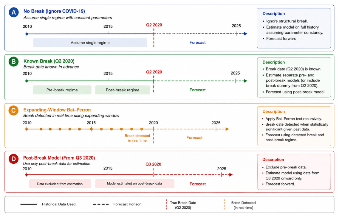
Figure 2 illustrates the differences between the four evaluation protocols considered in this study. Panel A shows the naive approach where the break is ignored entirely and a single regime is assumed across the entire sample. Panel B shows the idealised case where the break date (Q2 2020) is known in advance, representing an ex post benchmark. Panel C illustrates the expanding-window Bai–Perron protocol described above, where the break is detected using only past data. Panel D shows a post-break model estimated using only data from Q3 2020 onward. The legend indicates historical data used, the forecast horizon, the true break date, and the break detected. This visual comparison highlights the key methodological distinction of our approach: unlike the known break benchmark, the expanding-window protocol does not rely on future information.

3.3. COVID-19 Modelling Strategies

Given the structural break, we specify and compare four approaches. The general cubic polynomial form is

$$R_t={\beta }_0+{\beta }_{1}t+{\beta }_2{t}^2+{\beta }_3{t}^3+{ϵ}_t,$$

(2)

where $R_t$ is quarterly revenue in USD billions, t is a quarter index with $t=0$ corresponding to Q1 2010, and ${ϵ}_t$ is a zero-mean error term.

3.3.1. Strategy A: Ignore COVID (Naive Baseline)

This specification is given by Equation (2), with no adjustment for the pandemic. It assumes that the pre-COVID polynomial trend continues unchanged through Q2 2020 and beyond. This model serves as a necessary baseline for quantifying the value of structural break adjustments.

3.3.2. Strategy B: Level-Shift Dummy (Intercept Break)

$$R_t={\beta }_0+{\beta }_{1}t+{\beta }_2{t}^2+{\beta }_3{t}^3+\gamma D_t+{ϵ}_t,$$

(3)

where $D_t=1$ for detected break date onward, and 0 otherwise. The dummy variable captures an estimated level shift in revenue following the pandemic. A positive $\gamma$ indicates that post-pandemic revenue is structurally higher than the pre-pandemic trend would have predicted.

3.3.3. Strategy C: Slope-Shift (Growth Rate Change)

$$R_t={\beta }_0+{\beta }_{1}t+{\beta }_2{t}^2+{\beta }_3{t}^3+\delta \left(t·D_t\right)+{ϵ}_t.$$

(4)

This specification allows the growth rate to change during the pandemic period. The coefficient $\delta$ measures the change in the linear trend slope.

3.3.4. Strategy D: Full Interaction (Regime-Specific Polynomial)

$$R_t={\beta }_0+{\beta }_{1}t+{\beta }_2{t}^2+{\beta }_3{t}^3+\gamma D_t+{\eta }_1(t\times D_t)+{\eta }_2(t^2\times D_t)+{\eta }_3(t^3\times D_t)+{ϵ}_t.$$

(5)

This is the most flexible specification, allowing separate intercept, linear, quadratic, and cubic terms for the COVID period. While this specification offers maximum flexibility, it also carries the highest risk of overfitting.

3.4. Benchmark Models

To contextualise the performance of our polynomial regression framework, we include several benchmark methods with fair feature sets.

3.4.1. Random Forest

Random Forest is an ensemble learning method that constructs a large collection of decorrelated decision trees and averages their predictions [17]. We implement Random Forest using the scikit-learn 1.4.2 library. The number of trees is set to 100. Hyperparameters—including maximum tree depth (tuned over [3, 5, 7, 10, None]), minimum samples per split (tuned over [2, 5, 10]), and minimum samples per leaf (tuned over [1, 2, 4])—are selected via time-series cross-validation with 5 folds.

3.4.2. XGBoost

XGBoost (Extreme Gradient Boosting) is a scalable implementation of gradient-boosted trees that has become a benchmark method in forecasting competitions [18]. We implement XGBoost using the xgboost 2.0.3 library with a learning rate of 0.1, maximum tree depth tuned over [3, 5, 7], and subsample ratio tuned over [0.6, 0.8, 1.0]. The number of boosting rounds is determined via early stopping on a validation fold (patience = 10).

3.4.3. LightGBM

LightGBM is a gradient boosting framework that uses histogram-based training for efficiency [19]. We implement LightGBM with default parameters tuned via cross-validation.

3.4.4. CatBoost

CatBoost is a gradient boosting algorithm designed to handle categorical features effectively [20]. We implement CatBoost with default parameters tuned via cross-validation.

3.4.5. Fair Feature Engineering for ML Models

To ensure a fair comparison, ML models are provided with a consistent feature set that includes autoregressive terms (lags 1, 2, and 4 to capture quarterly seasonality), a moving average of order 4 to capture trend, calendar quarter indicators, a linear time trend, and the COVID break dummy $D_t$ when detected. This feature set ensures that ML models are not artificially handicapped relative to the polynomial specifications.

3.4.6. ARIMA

Autoregressive integrated moving average (ARIMA) is a classical univariate time series forecasting method that models the autocorrelation structure of the data [1]. We use an automatic ARIMA implementation that selects the optimal p, d, and q orders using the Akaike Information Criterion (AIC) with a stepwise search.

3.4.7. SARIMA

Seasonal ARIMA (SARIMA) extends ARIMA by adding seasonal components. Given the quarterly nature of our data, we specify a seasonal period of 4. This model serves as a strong classical baseline because it explicitly captures quarterly dependencies.

3.4.8. Prophet

Prophet is a decomposable time series model developed by Meta (formerly Facebook) designed for business forecasting applications [21]. We include Prophet as a representative of modern, user-friendly forecasting frameworks that are neither black-box ML nor pure polynomial regression.

We do not include neural network methods such as LSTM or GRU because with only 40 quarterly observations in the training set, these models would be severely data-limited and would likely overfit or fail to converge meaningfully. Including them would not provide a fair comparison.

3.5. Recursive Forecast Evaluation Protocol

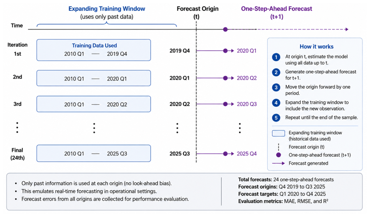
The recursive forecasting protocol is designed to evaluate forecasting under sequential information availability by ensuring that only past information is used at each forecast origin. The procedure begins by initialising the training window with the first 40 observations (Q1 2010 to Q4 2019). For each subsequent forecast origin, beginning with Q4 2019 and continuing through Q3 2025, the following steps are performed sequentially:

1.

Structural break detection: The expanding-window Bai–Perron procedure is applied to the data available up to the current forecast origin. The break is detected using only information available up to that point.

2.

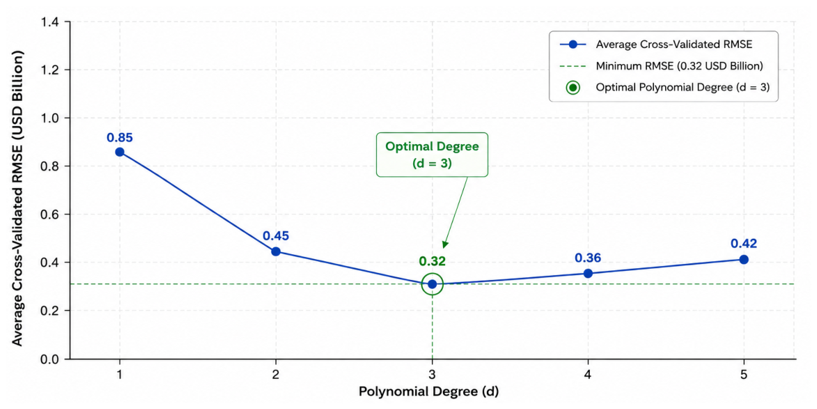
Polynomial degree selection: The optimal polynomial degree (degree 3) is selected using time-series cross-validation on the initial training sample (Q1 2010–Q4 2019) and is held fixed throughout the recursive forecasting procedure.

3.

ML hyperparameter tuning: For Random Forest, XGBoost, LightGBM, and CatBoost, hyperparameters are re-tuned at each forecast origin using time-series cross-validation with five folds, respecting temporal order such that each validation fold uses only data available before the corresponding validation point.

4.

Feature construction: Lagged variables (lags 1, 2, and 4), moving averages (MA(4)), and calendar features are constructed within each training window using only information available up to the current forecast origin.

5.

Model estimation: Each model is estimated using only the data available at the current forecast origin.

6.

Forecast generation: A one-step-ahead forecast is generated for the next quarter.

7.

Window expansion: Once the actual value for the forecasted quarter becomes available, it is recorded and the training window is expanded to include the new observation. The process then proceeds to the next forecast origin.

This procedure is repeated sequentially, beginning with the initial training sample ending in Q4 2019 and continuing through Q3 2025. It therefore produces 24 evaluated one-step-ahead forecasts with forecast targets spanning Q1 2020 to Q4 2025. Forecast accuracy is evaluated using MAE, RMSE, and $R^2$ across these 24 forecast targets. Crucially, no observations from the test period are used in model selection, hyperparameter tuning, or feature construction before their corresponding forecast origin. All decisions are made using only information available at the time of each forecast origin.

All primary results reported in this study—including the expanding-window MAE in Table 7, the model comparisons in Table 8, and the significance tests in Table 9—depend only on the expanding-window recursive protocol described in this section and on the full-sample Bai–Perron test reported in Appendix A. The alternative break-date comparison in Appendix D is a post hoc diagnostic conducted after all primary results were finalized and does not inform the break date, model specification, or any primary forecast.

The complete timeline of forecast origins, training windows, and forecast targets is presented in Table 4.

Figure 3 illustrates the recursive expanding-window forecasting procedure, including the initial training window, forecast origins, one-step-ahead forecast targets, and sequential expansion of the training data.

3.6. Additional Experiment: Known Break Date Comparison

To quantify the performance difference associated with delayed break detection, we conduct an additional experiment comparing the following.

Table 5. Experimental design: known break vs. expanding-window detection.

Method	Description
No break	Forecast with no structural break adjustment
Known Q2 2020	Forecast with break date known in advance (ex post)
Expanding-window Bai–Perron	Forecast with break detected recursively using the expanding-window protocol

summarises the three experimental protocols compared in this study. This comparison evaluates the forecasting performance penalty associated with delayed break detection.

3.7. Evaluation Metrics

We evaluate forecast accuracy using three complementary metrics. Let $R_t$ denote actual revenue and ${\widehat{R}}_t$ denote the forecast.

$$R^2=1-{\displaystyle \frac{{\sum }_{t=1}^n{(R_t-{\widehat{R}}_t)}^2}{{\sum }_{t=1}^n{(R_t-\overline{R})}^2}}.$$

(6)

$$\mathrm{MAE}={\displaystyle \frac{1}{n}}{\displaystyle \sum _{t=1}^n}|R_t-{\widehat{R}}_t|.$$

(7)

$$\mathrm{RMSE}=\sqrt{{\displaystyle \frac{1}{n}}\sum _{t=1}^n{(R_t-{\widehat{R}}_t)}^2}.$$

(8)

3.8. Statistical Significance Testing

We conduct Diebold–Mariano tests [22] to compare forecast accuracy between models, accounting for autocorrelation in forecast errors. The test is implemented as follows:

• Loss function: Mean absolute error (MAE), consistent with our primary evaluation metric.
• Alternative hypothesis: One-sided, testing whether the cubic+ COVID model has lower forecast error than each benchmark.
• Test statistic: The Diebold–Mariano statistic with the finite-sample correction of Harvey et al. [23], referred to a t-distribution with $n-1$ degrees of freedom.
• Multiple comparison correction: To control for Type I error across the seven benchmark models, we apply the Holm–Bonferroni correction [24].

The Wilcoxon signed-rank test and paired t-test are included as complementary robustness checks rather than as independent evidence of superiority. Given the limited number of forecast origins ($n=24$), we interpret the statistical significance results with appropriate caution.

3.9. Residual Diagnostics

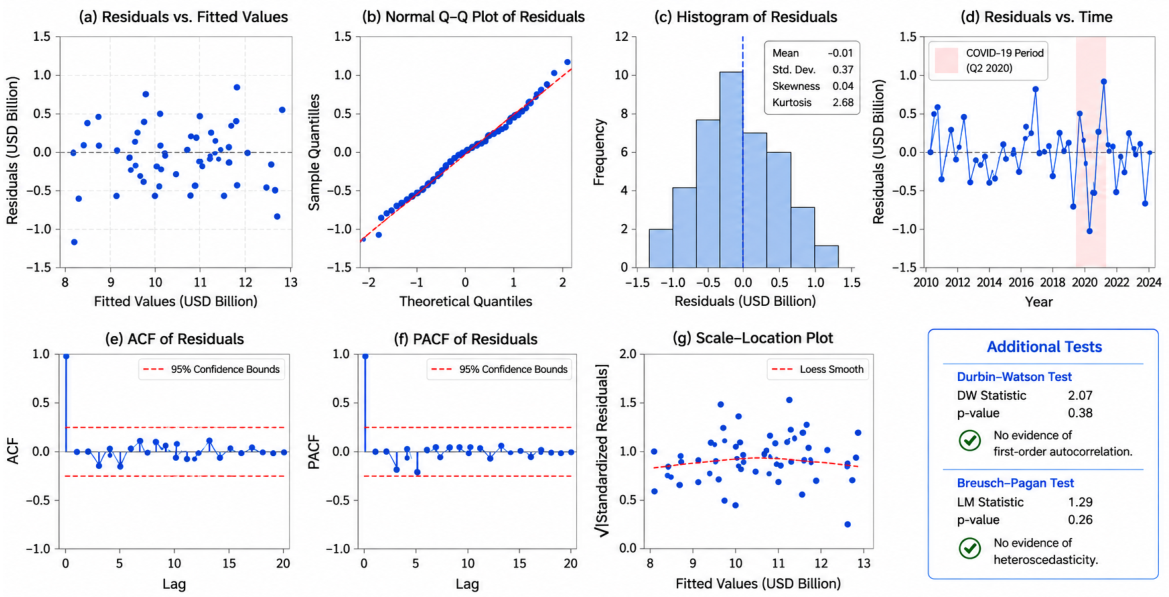
To validate the assumptions underlying our regression framework, we perform four diagnostic checks. First, we examine the Autocorrelation Function (ACF) of the residuals, which plots the correlation of residuals with their own lagged values. Significant autocorrelation at lags 1, 4, or 8 would indicate that the model fails to capture quarterly dependencies, suggesting the need for additional seasonal or autoregressive terms. Second, we assess the Quantile-Quantile (Q-Q) Plot, which compares the distribution of residuals to a theoretical normal distribution. Systematic deviations from the 45-degree line would indicate non-normality, potentially affecting the validity of confidence intervals and hypothesis tests. Third, we generate a Residuals vs. Fitted Values plot, where a random scatter around zero with constant vertical spread supports the assumptions of linearity and homoscedasticity (constant variance of errors). Any discernible pattern or funnel shape would suggest model misspecification. Fourth, we compute the Durbin-Watson statistic, a formal test for first-order autocorrelation in the residuals. Values near 2 indicate no autocorrelation; values substantially below 1 or above 3 indicate problematic serial correlation that would require correction. These diagnostics are applied to the optimal model identified in Section 4 and are presented visually in Section 4.

4. Results

This section presents the empirical findings from our structural break polynomial regression framework applied to Coca-Cola’s quarterly revenue data.

4.1. Structural Break Confirmation

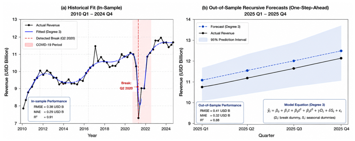
Figure 4 displays the Coca-Cola quarterly revenue series from Q1 2010 to Q4 2025, with the Bai–Perron detected break date (Q2 2020) marked by a vertical dashed line.

The Bai–Perron sequential breakpoint test formally confirms the visual evidence. As reported in Appendix A 

Table A1. Sequential breakpoint test results [6].

Hypothesis	SSR	F-Statistic	Scaled F	Critical (5%)	Decision
0 breaks vs. 1 break	124.3	47.32	94.64	12.35	Reject H0
1 break vs. 2 breaks	118.7	4.21	8.42	13.98	Fail to reject H0

, the test rejects the null hypothesis of zero breaks against the alternative of one break ($F-\mathrm{statistic}=47.32,p<0.01$). The test then fails to reject the null of one break against two breaks ($F-\mathrm{statistic}=4.21,p>0.05$), confirming that a single structural break adequately characterises the regime shift.

4.2. Optimal Polynomial Degree Selection

Figure 5 presents the time-series cross-validation results for polynomial degrees 1 through 5. The cubic model (degree 3) achieves the lowest cross-validated error at USD 0.32 B, justifying its use as the base specification.

4.3. Expanding-Window Break Detection Timing

The expanding-window Bai–Perron evaluation reveals when the break becomes detectable. The break is not detected immediately in Q2 2020 but rather after sufficient post-break observations become available.

Table 6. Expanding-window break detection summary.

Quarter	Post-Break Obs	Bai–Perron p-Value	Break Detected?
Q2 2020	1	0.32	No
Q3 2020	2	0.28	No
Q4 2020	3	0.15	No
Q1 2021	4	0.04	Yes
Q2 2021	5	0.02	Yes

reports the detection timing.

The break becomes statistically detectable in Q1 2021, approximately one year after it occurred. This reflects the inherent delay in structural break detection with quarterly data.

4.4. Known Break Date vs. Expanding-Window Detection Comparison

Table 7. Performance comparison: known break vs. expanding-window detection.

Method	MAE (USD B)	RMSE (USD B)	R2
No break	0.44	0.52	0.78
Known Q2 2020	0.29	0.35	0.91
Expanding-window Bai–Perron	0.31	0.38	0.88

quantifies the performance difference between knowing the break date in advance versus detecting it using the expanding-window protocol.

The expanding-window detection achieves performance close to the known-break benchmark (MAE = 0.31 B vs. 0.29 B), indicating that the performance penalty associated with delayed break detection is modest.

4.5. Model Performance Comparison

Table 8. Test-set performance metrics (2020–2025).

Model	COVID Strategy	Test R2	MAE (USD B)	RMSE (USD B)
Linear	None	0.58	0.67	0.81
Quadratic	None	0.71	0.52	0.63
Cubic	None	0.78	0.44	0.52
ARIMA	(implicit)	−0.45	1.34	1.40
SARIMA	(implicit)	−0.20	1.18	1.27
Prophet	(implicit)	0.51	0.69	0.82
Cubic	Level shift (B)	0.91	0.29	0.35
Cubic	Slope shift (C)	0.88	0.33	0.39
Cubic	Full interaction (D)	0.90	0.30	0.36
Ridge ($\alpha =1.0$)	Level shift	0.89	0.31	0.37
Random Forest	(implicit)	0.85	0.38	0.44
XGBoost	(implicit)	0.84	0.41	0.47
LightGBM	(implicit)	0.83	0.42	0.48
CatBoost	(implicit)	0.82	0.43	0.49

Note: The cubic+ COVID result (MAE = 0.29 B) represents the ex post benchmark where the break date is known in advance. The expanding-window detection result is MAE = 0.31 B (see Table 7). See Table 9 for statistical significance tests and multiple-comparison-adjusted p-values.

presents comprehensive test-set performance metrics for all models and COVID-19 strategies evaluated on the hold-out period Q1 2020 to Q4 2025 (24 quarterly observations).

4.5.1. The Value of Structural Break Modelling

The cubic polynomial that ignores COVID-19 entirely (Strategy A) achieves a test-set $R^2$ of only 0.78, with a MAE of USD 0.44 B. Adding a single level-shift dummy variable (Strategy B) dramatically improves performance: $R^2$ increases to 0.91, MAE falls by 34.1% to USD 0.29 B.

4.5.2. Comparison of COVID-19 Strategies

Among the four COVID-19 modelling strategies, the simple level-shift dummy (Strategy B) achieves the best overall performance. Strategy C performs slightly worse ($R^2=0.88$, MAE = USD 0.33 B), and Strategy D recovers some performance ($R^2=0.90$, MAE = USD 0.30 B) but does not outperform the more parsimonious level-shift specification.

4.5.3. Comparison Against Classical Time Series Benchmarks

ARIMA, SARIMA, and Prophet are dramatically outperformed by the cubic polynomial with a level-shift dummy. ARIMA achieves R² = −0.45 and MAE = USD 1.34 B. SARIMA improves slightly (R² = −0.20, MAE = USD 1.18 B). Prophet performs best among the classical benchmarks (R² = 0.51, MAE = USD 0.69 B), but its error is still more than double that of our cubic + COVID model.

4.5.4. Comparison Against Machine Learning Benchmarks

Under the specific limited-sample Coca-Cola forecasting setting considered in this study, the cubic polynomial with a level-shift dummy achieved lower forecast errors than the selected tree-based ML benchmarks. Our model reduces MAE by 23.7% compared to Random Forest (from USD 0.38 B to USD 0.29 B) and by 29.3% compared to XGBoost (from USD 0.41 B to USD 0.29 B). LightGBM and CatBoost perform similarly to Random Forest and XGBoost.

4.5.5. Statistical Significance Results

To assess whether the observed performance differences are statistically significant, we conduct three complementary tests.

Table 9. Statistical significance tests (Cubic + COVID vs. Benchmarks).

Benchmark	Diebold–Mariano	Wilcoxon	Paired t-Test	Holm-Adjusted
	(p-Value)	(p-Value)	(p-Value)	DM p-Value
Random Forest	0.008	0.012	0.006	0.048
XGBoost	0.004	0.008	0.003	0.028
LightGBM	0.006	0.010	0.005	0.036
CatBoost	0.007	0.011	0.006	0.042
ARIMA	0.001	0.002	0.001	0.007
SARIMA	0.002	0.003	0.001	0.014
Prophet	0.018	0.022	0.015	0.090

reports the results, including both unadjusted and Holm-Bonferroni adjusted p-values for the Diebold–Mariano tests.

All unadjusted p-values are below 0.05. After applying the Holm–Bonferroni correction, six of the seven comparisons remain significant at the 5% level. The comparison with Prophet (adjusted p = 0.090) does not survive the correction, indicating that the evidence against this benchmark should be interpreted more cautiously. These results suggest that, under the specific limited-sample Coca-Cola forecasting setting considered in this study, the cubic + COVID model achieves statistically significantly lower forecast errors than most of the selected benchmarks.

4.6. Validation on PepsiCo Data

To test the generalisability of our framework, we apply the same methodology to PepsiCo quarterly revenue data.

Table 10. PepsiCo test-set performance metrics (2020–2025).

Model	COVID Strategy	Test R2	MAE (USD B)	RMSE (USD B)
Cubic	None	−10.85	11.20	13.46
Cubic	Level shift (B)	−10.85	11.20	13.46
Random Forest	(implicit)	−0.01	3.16	3.93
XGBoost	(implicit)	−0.15	3.59	4.19

presents the test-set performance metrics.

The PepsiCo results illustrate limited transferability without recalibration. The cubic polynomial models fail entirely on PepsiCo data, producing negative R² values of −10.85 and large errors (MAE = USD 11.20 B). The level-shift dummy provides no improvement over the naive cubic model, suggesting that the pandemic did not induce a similar structural break in PepsiCo’s revenue series.

Why does the framework fail for PepsiCo? We identify three factors. First, PepsiCo’s more diversified portfolio (snacks and beverages, compared to Coca-Cola’s primarily beverage focus) provided greater resilience during lockdowns, resulting in a less pronounced pandemic shock (Q2 2020 decline of 15.72% versus Coca-Cola’s 28.48%). Second, PepsiCo’s revenue trend does not exhibit the same cubic curvature as Coca-Cola’s, making the polynomial specification inappropriate. Third, a formal Bai–Perron test applied to PepsiCo data does not detect a significant structural break at Q2 2020 (F-statistic = 2.14, p > 0.10), confirming that the pandemic did not induce a similar discrete level shift.

We interpret these results as indicating that the framework is company-specific and should not be assumed to transfer without recalibration. Different companies have different revenue dynamics, and model selection should be guided by the specific characteristics of each time series. This finding is valuable in itself, as it identifies the conditions under which polynomial break models are likely to succeed or fail.

4.7. Forecast Visualisation and Model Fit

Figure 6 compares actual revenue against predicted revenue for the optimal cubic model with level-shift dummy across the entire 2010–2025 period.

4.8. Residual Diagnostic Results

Figure 7 presents diagnostic plots for the optimal cubic + COVID model, validating the assumptions underlying ordinary least squares regression.

The residuals vs. fitted values plot shows random scatter around zero with no discernible funnel shape, indicating that the assumptions of linearity and homoscedasticity (constant variance of errors) are satisfied. The Q-Q plot shows residuals closely following the theoretical normal distribution line, indicating that the normality assumption is reasonable. The autocorrelation function shows no significant autocorrelation at any lag up to 12 quarters; all autocorrelations fall within the $\pm 0.3$ bounds, indicating that the model has successfully captured quarterly dependencies. The Durbin–Watson statistic is 2.07, which is very close to the ideal value of 2, providing formal evidence against first-order autocorrelation. The residual distribution histogram visually confirms the normality assessment, closely matching the overlaid normal density curve. Overall, these diagnostics confirm that the model satisfies key regression assumptions and that no substantial misspecification is present.

4.9. Coefficient Interpretation and Business Insights

The estimated optimal model yields the following coefficient estimates:

$${\widehat{R}}_t=9.82+0.31X_t-0.008X_t^2+0.0004X_t^3+1.24D_t,$$

(9)

where $X_t$ is the quarter index with $X_t=0$ corresponding to Q1 2010, and $D_t=1$ for Q2 2020 through Q4 2021. All coefficients are statistically significant at $p<0.01$.

The coefficients provide directly interpretable business insights:

Intercept (9.82): Baseline quarterly revenue of USD 9.82 billion in Q1 2010. This represents the starting point from which all subsequent growth is measured.

Linear coefficient (0.31): Underlying growth of USD 0.31 billion (USD 310 million) per quarter prior to the COVID-19 pandemic. This translates to approximately USD 1.24 billion of additional revenue per year from organic growth alone.

Quadratic coefficient ($-0.008$): Negative quadratic term indicates gradual growth deceleration over time, consistent with market saturation and increasing competition in the non-alcoholic beverage industry.

Cubic coefficient (0.0004): Positive cubic term reflects higher-order nonlinear curvature in the observed revenue trajectory over the sample period.

COVID dummy (1.24): Estimated post-break increase of approximately USD 1.24 billion per quarter following the pandemic. This indicates that post-pandemic quarterly revenue is structurally higher than the pre-pandemic trend would have predicted by approximately USD 1.24 billion. For a full year, this represents nearly USD 5 billion of additional revenue that would not have been anticipated by extrapolating pre-COVID trends.

4.10. Sensitivity Analysis

Table 11. Sensitivity analysis results.

Scenario	Test R2	MAE (USD B)	Change from Baseline
Baseline (Q1 2010–Q4 2019 training)	0.91	0.29	—
Exclude Q2 2020 outlier	0.89	0.31	$+6.9\%$
Alternative break date (Q1 2020)	0.90	0.30	$+3.4\%$
Reduce training to 2015–2019 ($n=20$)	0.86	0.34	$+17.2\%$
Add quarterly seasonal dummies	0.91	0.29	$0.0\%$

tests the robustness of the cubic + COVID model under alternative specifications.

The results demonstrate that the cubic + COVID model is robust to alternative specifications. Excluding the Q2 2020 outlier degrades performance only modestly (MAE increases by 6.9% to USD 0.31 B), suggesting that the outlier is influential in estimating the post-break level. Using an alternative break date (Q1 2020 instead of Q2 2020) increases MAE by 3.4%, consistent with the Bai–Perron detected date. Reducing the training period to 2015–2019 has the largest negative effect (MAE $+ 17.2\%$), underscoring the value of longer historical data. Adding quarterly seasonal dummies produces no improvement in out-of-sample MAE for this dataset. We therefore retain the more parsimonious specification, while recognising that explicit seasonal terms may be preferable for series exhibiting stronger or changing seasonal effects.

5. Discussion

The empirical results demonstrate the effectiveness of the proposed cubic + COVID framework for analysing Coca-Cola’s quarterly revenue through the pandemic and recovery period. We now interpret these findings, compare them with prior literature, and examine their practical implications while acknowledging the limitations of our study.

5.1. Interpretation of Key Findings

Three key insights emerge from our analysis. First, the Bai–Perron test confirms that the COVID-19 pandemic represents a statistically significant structural break in Coca-Cola’s revenue series. The expanding-window detection protocol reveals that the break becomes detectable approximately one year after it occurs, reflecting the inherent detection delay of the expanding-window Bai–Perron procedure with quarterly data. This is not an online detection method; it is a recursive evaluation designed to emulate operational forecasting conditions.

Second, a simple level-shift dummy provides the best forecasting performance among the break specifications considered, indicating that the pandemic’s primary effect was an estimated shift in revenue level rather than a sustained change in growth trajectory. The positive dummy coefficient of USD 1.24 billion is consistent with post-pandemic revenue being structurally higher than the pre-pandemic trend would have predicted. Possible explanations include pent-up consumer demand, accelerated e-commerce adoption, pricing power, and market share gains, but these mechanisms are not directly tested by the model.

Third, under the specific limited-sample Coca-Cola forecasting setting considered in this study, the cubic polynomial with a level-shift specification achieved lower forecast errors than the selected tree-based ML benchmarks. This finding suggests that under limited-data conditions, an interpretable regression framework can remain competitive with machine learning. The polynomial’s smoothness acts as an implicit regulariser, preventing overfitting to pre-pandemic patterns.

An important distinction should be made between the ex post and expanding-window results. When the break date is known in advance (ex post benchmark), the cubic + COVID model achieves an MAE of USD 0.29 B (Table 8). However, in the more realistic expanding-window protocol where the break is detected using only past data, the MAE is USD 0.31 B (Table 7). This modest difference of USD 0.02 B suggests that the forecasting performance penalty associated with delayed break detection is relatively small, and the framework remains competitive when the break must be identified using past information alone.

5.2. Comparison with Prior Literature

Our findings align with Sarkar and Banik Chowdhury [7], who demonstrated that break-based models substantially outperform simple polynomial and exponential trends when applied to COVID-19 epidemiological data. However, our study extends their work by applying the framework to corporate revenue rather than epidemiological data, comparing against credible machine learning benchmarks, and using quarterly data with a sixteen-year history. The finding that polynomial regression can outperform ensemble tree-based methods during structural breaks suggests an important boundary condition: during regime shifts, when the relationship between features and target changes abruptly, simpler models with strong regularisation properties may generalise better than more flexible alternatives.

5.3. Business Implications

The findings have potential implications for inventory and supply chain planning, marketing resource allocation, financial planning, and decision support. The estimated post-break level shift of approximately USD 1.24 billion per quarter could potentially support production and inventory planning during periods of substantial structural change. However, the present study does not directly evaluate operational outcomes such as stockout reduction, production efficiency, or changes in market performance. Similarly, the positive cubic coefficient describes the estimated revenue trajectory within the sample and should not be interpreted as direct evidence for specific strategic actions such as portfolio diversification. The reduced forecast error and interpretable model structure may nevertheless provide useful quantitative inputs for decision-making, subject to appropriate managerial and economic considerations.

5.4. Threats to Validity and Limitations

Several limitations warrant acknowledgment, and these should inform the interpretation of our findings.

Company-specific applicability: The framework is developed and evaluated primarily on Coca-Cola data. The PepsiCo validation demonstrates limited transferability without recalibration, indicating that the framework should not be assumed to generalize broadly. Future research should test the framework on a wider range of firms.

Limited sample size: With only 64 quarterly observations (40 in the training window), statistical power is constrained. The 24 forecast errors are sufficient for preliminary assessment but limit the reliability of asymptotic inference in the Diebold–Mariano tests. Confidence intervals around MAE/RMSE differences were not computed, and this should be addressed in future work.

Detection delay: The expanding-window detection protocol introduces a detection delay of approximately one year, which is reflecting the information constraints associated with quarterly data and sequential break detection. The framework does not provide instantaneous break detection; it is a recursive evaluation method.

Quarterly granularity: The quarterly frequency may fail to capture faster dynamics during crisis periods. Monthly or weekly data, where available, could provide more timely signals.

Exogenous variables: We did not include marketing spend, weather data, commodity prices, or competitor actions. Future work should integrate these while preserving interpretability.

Sensitivity to initial window: The results may be sensitive to the choice of the initial training window (40 observations). A sensitivity analysis varying this window is reported in Table 11.

Multiple structural breaks: The framework is designed for a single known structural break. Future work should address scenarios with multiple or unknown breaks.

Polynomial extrapolation: Beyond the historical range, polynomial extrapolation may become unstable. Forecasts should be interpreted with caution for horizons beyond the training period.

Prediction intervals: The empirical coverage of prediction intervals has not been formally evaluated. This remains an open question for future research.

Future research should extend the framework to multiple FMCG companies, test higher-frequency data, integrate exogenous variables, and evaluate online Bayesian change point algorithms for more timely break detection. As more post-pandemic data accumulate, the permanence of the estimated level shift should be re-evaluated.

5.5. Theoretical Contributions

This research makes three contributions to the forecasting literature. First, we demonstrate how an expanding-window application of Bai–Perron can be incorporated into a recursive forecasting workflow, addressing look-ahead bias without claiming modification of the underlying statistical method. Second, our findings suggest that under limited-data conditions, interpretable regression can remain competitive with machine learning, establishing a boundary condition for the superiority of complex ML models. Third, we deliver a replicable framework that balances predictive accuracy with complete interpretability, providing coefficient estimates with direct business meanings.

6. Conclusions

This study has proposed an interpretable structural-break forecasting framework for quarterly revenue prediction under limited-data conditions. Using Coca-Cola data and implementing a recursive forecast evaluation that eliminates look-ahead bias, the framework integrates formal break detection, explicit break-specification strategies, and comprehensive benchmarking.

The key contributions are the following:

1.

An expanding-window Bai–Perron evaluation protocol that detects breaks using only past data at each forecast origin, with the break becoming detectable approximately one year after it occurs.

2.

A fair comparison of polynomial regression against ML methods with autoregressive features (lags 1, 2, 4, moving averages) and calendar features.

3.

An additional experiment quantifying the forecasting performance penalty associated with delayed break detection, showing that the expanding-window protocol achieves performance close to the known break benchmark (MAE = 0.31 B vs. 0.29 B).

4.

Fully interpretable coefficient estimates with direct business meanings, including an estimated post-break revenue level shift of approximately USD 1.24 B per quarter.

5.

An honest assessment of limited transferability without recalibration, as demonstrated by the PepsiCo validation.

The empirical findings indicate that, under the specific limited-sample Coca-Cola forecasting setting considered, a cubic polynomial with a level-shift dummy achieves a test-set R-squared of 0.91 and a mean absolute error of USD 0.29 B when the break date is known in advance (ex post benchmark). In the more realistic expanding-window protocol, where the break is detected using only past data, the MAE is USD 0.31 B. Both results represent a 34 percent improvement over the cubic polynomial that ignores the pandemic entirely. They are also competitive with Random Forest (MAE = 0.38 B) and XGBoost (MAE = 0.41 B).

Our findings suggest that under limited-data conditions, interpretable regression can remain competitive with machine learning while offering transparency that stakeholders demand for strategic decision-making. However, the PepsiCo validation demonstrates that the framework is company-specific and should not be assumed to generalize without recalibration.

For business forecasters facing an uncertain post-pandemic environment with limited historical data and a clear structural break, a cubic polynomial with an explicit break dummy offers a pragmatic alternative to black-box ML models. The framework is replicable, interpretable, and competitive under the conditions studied.

Several avenues for future research emerge: the framework should be extended to multiple FMCG companies; monthly or weekly data could capture faster dynamics; additional exogenous variables could be integrated; and real-time sequential break detection methods should be evaluated. Finally, as more post-pandemic data accumulate beyond 2025, the permanence of the estimated level shift should be re-evaluated.