Article

Forecasting the Evolving Composition of Guest Origin Markets in Platform Bookings: A Bayesian Compositional Time-Series Approach Using Airbnb Data

Finance Data Science & Strategy, Airbnb Inc., San Francisco, CA 94103, USA
Forecasting 2026, 8(4), 74; https://doi.org/10.3390/forecast8040074
Submission received: 27 June 2026 / Revised: 8 August 2026 / Accepted: 14 August 2026 / Published: 16 August 2026

Highlights

What are the main findings?
  • BDARMA achieves the lowest forecast error for EMEA, cutting mean absolute error by 27% relative to naive forecasts (p < 0.001), but simple benchmarks remain hard to beat in the other three regions, so direct compositional modeling pays off mainly where several origin markets hold material shares.
  • Introducing seasonal structure in the Dirichlet precision parameter lowers mean absolute error in all four destination regions, by 13% to 35% relative to an otherwise identical constant-precision specification.
What are the implications of the main findings?
  • Because the target is monthly booking composition indexed by booking date rather than stay date, the forecasts are observable ahead of realized arrivals and can support source-market budget allocation, concentration-risk monitoring, and operational planning at the lead times those decisions require.
  • Model complexity should be matched to market structure rather than assumed: compositional modeling earns its cost in diverse origin portfolios, while simpler methods stay competitive where one origin dominates or a smooth recovery path carries most of the signal.

Abstract

Tourism-demand forecasting overwhelmingly targets aggregate volumes, leaving the question of where demand will come from largely unaddressed. This paper forecasts that question directly. We make three contributions. First, we apply Bayesian Dirichlet autoregressive moving average (BDARMA) models to guest origin composition in large-scale platform booking data, which to our knowledge is the first use of Bayesian compositional time-series methods on booking-origin shares across multiple global destination regions. Second, we introduce seasonal structure in the Dirichlet precision parameter, and we isolate its contribution through an ablation against an otherwise identical constant-precision specification: seasonal precision lowers mean absolute error in all four destination regions, by between 13% and 35%. Third, the forecast target is the monthly composition of bookings indexed by booking date rather than stay date, which makes it observable ahead of realized arrivals and therefore usable for decisions with long lead times. Using proprietary Airbnb reservation data spanning 2017–2025 across four destination regions, we document substantial pandemic-era shifts in booking composition with heterogeneous recovery patterns. In rolling-origin evaluation, BDARMA achieves the lowest forecast error for EMEA, the most compositionally diverse region, reducing mean absolute error by 27% relative to naïve forecasts ( p < 0.001 ). Performance elsewhere is mixed: simple benchmarks remain hard to beat, and exponential smoothing on isometric log-ratio-transformed data attains the lowest error averaged across the four regions. The EMEA pattern suggests that direct compositional modeling is most valuable where several origin markets hold material shares, although four destination regions are too few to establish this as a general rule. The methodology yields probabilistic forecasts of source market shares that can inform marketing allocation, concentration-risk monitoring, and forward-looking operational planning.

1. Introduction

Tourism-demand forecasting has long been recognized as essential for destination planning, resource allocation, and strategic decision-making [1,2]. Accurate forecasts enable destination marketing organizations (DMOs) to optimize promotional spending across source markets, allow hospitality businesses to adjust pricing, staffing, and service design, and help destination analysts monitor shifts in market mix [3,4]. While the tourism-forecasting literature is extensive, the vast majority of studies focus on predicting aggregate arrivals or total expenditure [5,6]. Considerably less attention has been paid to forecasting the composition of demand, that is, how the mix of visitors from different origin markets evolves over time.
To see why origin composition matters independently of aggregate volume, consider a DMO setting its source-market campaign budgets for the coming year. The relevant question is not only how many visitors may ultimately arrive, but what the evolving booking mix suggests about where they are likely to come from, because the allocation decision must be made months before stays materialize. A forecast that the German share of current booking flows is trending upward while the UK share is declining for a Mediterranean destination justifies redirecting spend toward German-market campaigns, travel fair partnerships, and airline co-marketing before the season opens, not after it closes.
Two further decisions have the same structure. Origin composition is a measure of strategic risk, because a destination whose booking mix concentrates in a single source market accumulates fragility that aggregate volume forecasts conceal, as the collapse of Chinese-origin bookings into the Asia-Pacific made concrete. It also drives operational planning, because staffing, amenity, and service decisions are difficult to reverse mid-season. Section 6 develops all three in detail against the empirical results.
In this paper, the forecast target is the monthly composition of reservations by guest origin indexed by booking date, not the composition of realized arrivals or stays indexed by check-in month. That distinction matters. Booking-month composition can serve as a leading indicator for destination managers because it is observed earlier than realized arrivals, but it also reflects changes in booking timing and platform usage. We therefore interpret the series as booking demand on Airbnb, not as a census of realized inbound tourism demand.
The composition of booking demand also presents a distinct methodological challenge. Visitors from different source markets exhibit distinct spending patterns, budget allocations, and demand sensitivities [7,8], and geopolitical events, exchange rate fluctuations, and public health crises affect origin markets asymmetrically [9,10]. Capturing these dynamics requires methods that respect the constraints inherent in compositional data: origin market shares must sum to unity and each share is bounded between zero and one. Standard time-series methods that ignore these constraints can produce incoherent forecasts, for example, predicted shares that sum to more than 100% or take negative values [11,12].
Two families of methods respect the constraint, and the difference between them is where the coherence comes from. The compositional data analysis literature, pioneered by Aitchison [13], maps the simplex to unconstrained Euclidean space through log-ratio transformations, applies standard multivariate machinery there, and maps back. This works, and two of our benchmarks are built exactly this way. The approach has costs. Because the back-transformation is nonlinear, a symmetric interval in log-ratio coordinates is asymmetric on the simplex, interpretation in terms of shares is indirect, and performance can degrade when shares approach zero [14]. In the standard formulations used as benchmarks below, predictive dispersion follows from the transformation and the fitted error variance rather than from a separately specified process, though richer transformed families can parameterize covariance directly.
The alternative places a distribution directly on the simplex. The Dirichlet is the canonical choice, and three of its properties motivate its use here. Its support and the sample space of the data coincide, so every posterior predictive draw is a valid composition and no post hoc normalization is required. Its concentration parameter is a free quantity, which means predictive dispersion can be modeled rather than implied, and it is precisely this feature that permits the seasonal precision specification we introduce in Section 3. And because the model is specified on the compositions themselves, its parameters retain an interpretation in terms of shares. We apply the Bayesian Dirichlet Autoregressive Moving Average (BDARMA) framework of Katz et al. [15] to this setting; Section 2 reviews the relevant methodological background.
This paper contributes to both the tourism-forecasting and compositional time-series literatures by developing and applying BDARMA models to forecast guest origin market shares in large-scale platform booking data. We analyze Airbnb reservations from 2017 to 2025 across four major destination regions (EMEA, North America, Asia-Pacific, and Latin America), providing what is, to our knowledge, the first application of Bayesian compositional time-series methods to large-volume platform booking-origin shares across multiple global destination regions.
Our empirical setting offers several advantages. First, Airbnb operates globally with standardized data collection, enabling consistent measurement across diverse markets. Second, platform booking data capture actual reservations rather than survey-based intentions or aggregate border-crossing statistics, providing a direct measure of revealed booking demand. Because reservations are indexed by booking date rather than check-in date, the series provide an earlier signal of changing market mix, even though they are not identical to realized stay-month demand. Third, our sample period spans the COVID-19 pandemic and subsequent recovery, allowing us to examine how compositional dynamics shifted during and after this unprecedented disruption. Prior work using Airbnb data has examined other dimensions of pandemic-era booking behavior, but the evolution of origin market composition has not been systematically analyzed.
We find that BDARMA models achieve the lowest forecast error for EMEA, the most compositionally diverse destination region, while simpler benchmarks remain difficult to beat in the other three regions, a pattern consistent with a long-standing finding in the tourism-forecasting literature. The pandemic caused dramatic compositional shifts in booking flows, most notably a surge in within-region booking shares at the expense of long-haul markets, with recovery trajectories that varied markedly across destination regions. Our models capture these dynamics through autoregressive and moving average terms that allow past compositions and shocks to influence current shares, while the Dirichlet likelihood ensures forecasts remain valid probability distributions.
Seasonal variation in the precision parameter improves point accuracy in every region, which we establish in Section 5.4 through a direct comparison against an otherwise identical constant-precision model.
The remainder of this paper is organized as follows. Section 2 reviews related work on tourism-demand forecasting, compositional data analysis, and peer-to-peer accommodation research. Section 3 presents the BDARMA modeling framework and estimation approach. Section 4 describes our Airbnb booking data and the construction of origin market compositions. Section 5 reports empirical findings, including model comparisons and forecast accuracy assessments. Section 6 discusses implications for destination management and directions for future research. Section 7 concludes.

2. Literature Review

2.1. Tourism-Demand Forecasting

Tourism-demand forecasting is a methodologically mature field, with a long line of work spanning econometric demand models, time-series benchmarks, and more recent machine learning and hybrid approaches [1,3,5,16]. Most studies forecast scalar outcomes such as arrivals, overnights, or expenditure, typically using income, relative prices, exchange rates, and other macroeconomic drivers as core predictors [2,3]. Song et al. [17] and Li et al. [18] show that time-varying parameter formulations and related structural-change mechanisms can improve forecast accuracy when demand relationships evolve over time. Table 1 summarizes the principal methodological strands, the settings in which they have been applied, how each handles compositional structure, and the central finding associated with each.
A durable finding in this literature is that simple baselines are difficult to beat consistently. The tourism-forecasting competition showed that naïve and automated univariate methods remain powerful comparators, and subsequent work has emphasized forecast combination and stabilization rather than assuming that more complex models will dominate mechanically [19,20,21]. This is important for the present study because any new compositional forecasting framework should be evaluated against strong, parsimonious benchmarks rather than only against weak strawman alternatives.
A second major development is the expansion of the information set through digital traces and other high-frequency data. Internet search intensity, multisource big data, online reviews, and mixed-frequency indicators have all been shown to improve tourism forecasts, especially at short horizons and during disrupted periods [22,23,24,25,26]. At the same time, recent work cautions that search-based forecasting is sensitive to query design, preprocessing, and model specification [27]. For the present paper, this literature is relevant because it demonstrates that tourism forecasting increasingly relies on data that capture changing market structure earlier and more granularly than official statistics alone.
Machine learning and hybrid approaches occupy a growing share of this literature. Neural architectures, support vector regression, and ensembles combining statistical and learned components have been applied to arrivals forecasting with mixed results [5,16,22]. The pattern that emerges is conditional rather than uniform: gains concentrate where the information set is wide, where series are long enough to support the parameter counts involved, or where a panel of related series permits cross-learning. In short monthly series of the kind studied here, the competition evidence continues to favor parsimony [19]. We return to this point in Section 6 when considering the comparator set.
The pandemic made regime instability a first-order forecasting problem. COVID-19 did not simply reduce aggregate travel volumes; it changed the composition of travel across origins, trip types, and planning horizons, which in turn increased interest in adaptive models, external information, and explicit evaluation under disruption [9,10,16,36]. Yet, despite this progress, the dominant forecasting targets in tourism remain aggregate volumes rather than the evolving composition of demand itself. In that sense, forecasting origin-market shares extends a recent concern in the tourism-forecasting literature: understanding not only how much tourism demand will materialize, but how that demand is redistributed across source markets when conditions change.
Despite this rich literature, forecasting the composition of tourism demand, as opposed to aggregate levels, has received limited attention. A notable exception is the almost-ideal demand system (AIDS) and related demand-system approaches [7,18], which model budget shares allocated to different tourism products, destinations, or source markets. However, demand-system approaches focus on expenditure allocation rather than visitor origin shares per se, and standard linear specifications do not naturally enforce simplex constraints.
At the same time, the platform accommodation literature has devoted far more attention to market impacts, pricing, governance, and regulation than to forecasting per se. This leaves a gap at the intersection of platform research and tourism forecasting: platform booking data are timely and behaviorally rich, but forecasting applications remain few and have targeted occupancy, demand volume, and prices [32,33,34,35] rather than how tourism demand is redistributed across source markets over time [1,16,37,38].

2.2. Compositional Data Analysis

Compositional data, observations that represent parts of a whole and thus sum to a constant, arise throughout the sciences [11]. The standard approach transforms compositions via log-ratios (additive, centered, or isometric) to map the simplex to Euclidean space, after which conventional multivariate methods apply [12,29]. For time series, this enables the use of vector autoregression (VAR) and related models on transformed data [28].
An alternative approach models compositions directly using distributions supported on the simplex. The Dirichlet distribution is the canonical choice, parameterized by a concentration vector α = ( α 1 , , α C ) with α c > 0 . Grunwald et al. [30] proposed Bayesian state-space models for continuous proportions, while Zheng and Chen [31] developed frequentist Dirichlet ARMA models. More recently, Katz et al. [15] introduced the Bayesian Dirichlet ARMA (BDARMA) framework, which combines the Dirichlet likelihood with vector autoregressive moving average (VARMA) dynamics on the mean parameters.
The BDARMA framework offers several advantages for tourism applications. First, forecasts automatically satisfy simplex constraints without post hoc normalization. Second, the Dirichlet concentration parameter provides a natural measure of forecast uncertainty: lower concentration implies greater dispersion across possible compositions. Third, the Bayesian approach yields full posterior predictive distributions, enabling probabilistic statements about future market shares.

2.3. Peer-to-Peer Accommodation and Platform Data

The rise of peer-to-peer (P2P) accommodation platforms, particularly Airbnb, has transformed the hospitality landscape and generated a substantial research literature [39,40,41]. Studies have examined Airbnb’s competitive effects on hotels [37], and implications for destination governance [42].
A small body of work has taken Airbnb activity itself as the forecast target, and it is worth engaging with directly because it shapes how our results should be read. Gunter and Önder [32] model the determinants of Airbnb demand in Vienna alongside its interaction with the traditional accommodation sector, and Gunter et al. [33] extend the program to New York City with listing-level spatial panel methods, establishing that platform demand responds to economic fundamentals in ways stable enough to support model-based prediction. Milone et al. [34] trace how pandemic policy stringency propagated into European listing prices. The closest antecedent to the present paper is Gunter et al. [35], who model and forecast Airbnb occupancy for 43 European countries during the pandemic and find that a seasonal Markov-switching autoregression performs especially well in that period because it pairs detection of the pandemic-induced structural break with explicit seasonal structure. That is a sharp diagnosis. It anticipates a central pattern in our own results, where forecast accuracy under the pandemic regime shift hinges on exactly this combination of adaptation and seasonality (Section 5). The targets in this literature are occupancy, demand volume, and price; the composition of platform demand across origin markets has not yet been a forecast target, and it is the object of interest here.
Platform data offer unique advantages for tourism research. Unlike official statistics that rely on border crossings or accommodation surveys, booking data capture actual reservations with precise timing and geographic detail. When indexed by booking date, they also embed information about booking lead times, which can shift meaningfully over time.
Katz et al. [43] analyzed booking lead time distributions across major U.S. cities during the pandemic, finding a two-phase pattern of disruption followed by incomplete recovery, which is the empirical basis for distinguishing booking-month from stay-month composition throughout this paper. Sainaghi and Chica-Olmo [38] examined revenue impacts in Milan.
Three literatures therefore meet without overlapping. Tourism forecasting has developed sophisticated machinery for aggregate volumes but has largely left composition aside, treating the mix of origins as context rather than as a forecast target. Compositional data analysis has produced time-series models that respect the simplex, including Dirichlet-based specifications with full predictive distributions, but these have been applied to lead times, asset shares, and other domains rather than to tourism demand. Platform research has established that booking data are timely and behaviorally rich, and has begun to use them for prediction, but the targets have been occupancy, volume, and price. The gap is the intersection: a compositional forecast target, drawn from platform booking data, evaluated against the operational benchmarks the tourism literature has shown to be hard to beat. That is what this paper supplies.

3. Methodology

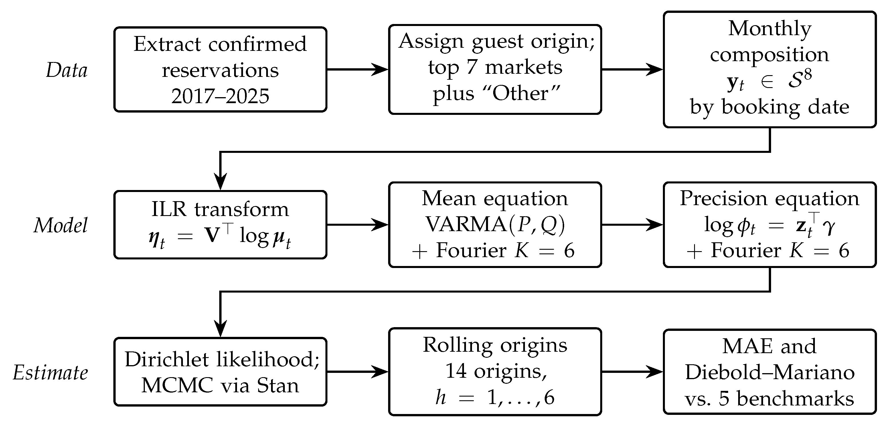
Figure 1 summarizes the analytical workflow, from reservation extraction through compositional construction, model specification, estimation, and rolling-origin evaluation. The subsections that follow develop each stage.

3.1. The BDARMA Model

Let y t = ( y t , 1 , , y t , C ) denote the vector of origin market shares at time t, where y t , c 0 and c = 1 C y t , c = 1 . We model y t as Dirichlet-distributed conditional on time-varying parameters:
y t μ t , ϕ t Dirichlet ( ϕ t μ t ) ,
where μ t = ( μ t , 1 , , μ t , C ) is the mean composition satisfying c = 1 C μ t , c = 1 , and ϕ t > 0 is the precision (concentration) parameter. Under this parameterization, E [ y t ] = μ t and Var ( y t , c ) = μ t , c ( 1 μ t , c ) / ( 1 + ϕ t ) .
To model temporal dynamics, we work with the isometric log-ratio (ILR) transformation of the mean:
η t = ILR ( μ t ) = V log ( μ t ) ,
where V is a C × ( C 1 ) contrast matrix satisfying V V = I C 1 and V 1 C = 0 . The ILR transformation maps the C-part simplex to R C 1 while preserving the geometry of compositional data [29]. The inverse transformation recovers μ t via the generalized softmax. We use the Helmert contrast basis throughout. The contrast matrix V is held fixed across all models, regions, and forecast origins, so every comparison below is made in a common coordinate system. Because the autoregressive priors below distinguish diagonal from off-diagonal elements, the prior specification is not invariant to the choice of basis, and results are conditional on this fixed basis.
The BDARMA ( P , Q ) specification determines η t through a VARMA-type recursion driven by the ILR-transformed observations:
η t = X t β + p = 1 P A p ILR ( y t p ) X t p β + q = 1 Q B q ϵ t q ,
where X t is a covariate matrix (including Fourier terms for seasonality), β contains regression coefficients, A p are ( C 1 ) × ( C 1 ) autoregressive coefficient matrices, B q are moving average coefficient matrices, and ϵ t = ILR ( y t ) η t are ILR-scale residuals. Both sums are functions of past observed compositions rather than of lagged latent means, in the manner of generalized autoregressive moving average models, so the recursion is available in closed form at estimation time and is iterated forward at forecast time by substituting posterior predictive draws for unobserved lags. These innovations do not have conditional mean zero under the Dirichlet likelihood; Appendix A states the bias and an available centered correction.

3.2. Seasonal Precision

A key modeling choice is whether the precision parameter varies over time. We allow the precision to depend on seasonal covariates:
log ϕ t = z t γ ,
where z t includes an intercept and Fourier terms ( K = 6 harmonics) capturing monthly seasonality. The same K = 6 harmonic set enters the mean covariates X t . At the monthly frequency, this is a saturated seasonal representation, equivalent in span to calendar-month effects; the sine harmonic at the Nyquist frequency is identically zero at integer monthly indices, so the seasonal block spans eleven nontrivial harmonic columns. This specification allows compositional volatility to vary seasonally, for example, summer months may exhibit tighter concentration around expected shares due to more predictable booking patterns, while shoulder seasons may show greater dispersion.
The specification is motivated by the descriptive evidence in Section 4 and evaluated directly in Section 5.4, where we compare it against an otherwise identical model in which the precision equation is reduced to an intercept, so that log ϕ t = γ 0 . That comparison isolates the contribution of the seasonal precision structure while holding the data, the ILR basis, the mean specification, the autoregressive and moving average orders, the priors, and the estimation settings fixed.

3.3. Prior Specification

We adopt weakly informative priors: for the intercept and regression coefficients, we use β j Normal ( 0 , 1 ) . For autoregressive coefficients, we place Normal ( 0.5 , 0.3 ) priors on diagonal elements (reflecting typical persistence) and Normal ( 0 , 0.2 ) on off-diagonal elements. Moving average coefficients receive Normal ( 0 , 0.3 ) priors. The precision intercept has a Normal ( 3 , 1 ) prior, implying moderate concentration, with seasonal coefficients receiving Normal ( 0 , 0.5 ) priors. The constant-precision specification of Section 5.4 retains the same precision-intercept prior, so the two arms of the ablation differ only in the presence of the seasonal harmonic columns.

3.4. Estimation

We estimate the model using Markov chain Monte Carlo (MCMC) via Stan [44], accessed through the darma R package (version 0.1.0), which requires R 4.1 or later and calls CmdStan 2.33 or later through cmdstanr 0.7.0 or later. We run four chains for 2000 iterations each (1000 warmup), yielding 4000 posterior draws. Convergence is assessed via the R ^ statistic and effective sample size [45].

3.5. Forecasting and Evaluation

Given posterior draws of model parameters, we generate h-step-ahead forecasts by iterating the VARMA recursion forward and sampling from the implied Dirichlet predictive distribution. Point forecasts are posterior means of the predictive composition; interval forecasts use posterior quantiles.
Our empirical evaluation focuses primarily on point-forecast accuracy. Specifically, we compute the mean absolute error (MAE) averaged across components, and this metric underlies the benchmark tables and Diebold–Mariano tests reported in Section 5. A fuller probabilistic assessment using log predictive density, interval coverage, and formal calibration analysis is important, but it lies beyond the scope of the present paper.
We compare BDARMA against five benchmarks: (i) naïve forecasts (last observation carried forward); (ii) seasonal naïve (same month previous year); (iii) rolling mean (12-month average); (iv) exponential smoothing (ETS) fitted to the ILR-transformed compositional series; and (v) SARIMA fitted to the ILR-transformed compositional series. The last two are the log-ratio comparators the compositional literature treats as standard practice: each ILR coordinate is modeled with automatic order selection, refitted at every forecast origin, and the fitted values are returned to the simplex by the inverse ILR transformation so that all forecasts are compared on a common scale. These are strong comparators rather than strawmen, and ETS in particular attains the lowest error averaged across the four regions. If anything, the design tilts toward the benchmarks: their structure is re-selected at every forecast origin while the BDARMA orders stay frozen. The set is intended to cover widely used operational baselines rather than to exhaust the space of multivariate or compositional competitors.
Model comparison within the BDARMA family uses leave-one-out cross-validation (LOO-CV) via Pareto-smoothed importance sampling [46]. We report the expected log pointwise predictive density (ELPD) and effective number of parameters ( p loo ). To test whether accuracy differences between methods are statistically significant, we employ the Diebold–Mariano test [47]; details are provided in Appendix A.

4. Data

4.1. Airbnb Booking Data and Forecast Target

Our analysis uses reservation data from Airbnb’s global platform spanning January 2017 through December 2025. Airbnb is one of the world’s largest peer-to-peer accommodation marketplaces, operating in over 220 countries and regions with more than 9 million active listings [48]. The platform’s standardized booking infrastructure enables consistent measurement of guest origin and destination across diverse markets.
Reservations are extracted from Airbnb’s internal bookings data warehouse, which records one row per reservation event with the booking date, the guest’s registered country of residence, and the listing’s destination country and region. We restrict to confirmed reservation events, excluding cancellations, and aggregate to monthly frequency by booking month, destination region, and guest origin country. The full sample comprises 108 monthly observations per destination region. Guests are assigned to origin countries by registered country of residence at the time of booking, which is the platform’s own account-level field rather than an inferred location.
Cancellation status is applied ex post: a reservation booked in month t and subsequently canceled is excluded from month t’s composition, so the historical series reflect final booking status rather than the exact information set available in real time, and the leading-indicator interpretation developed below should be read accordingly.
The time index in our analysis is the month in which the reservation is booked, not the month of check-in or realized stay. Accordingly, each composition in the paper should be read as the share of bookings made in month t that comes from each origin market. This makes the series useful as a forward-looking indicator of demand mix because bookings are observed before stays occur, but it also implies that the object of interest is booking composition rather than realized arrival-month tourism demand. When booking lead times shift, as they did during and after COVID-19 [43], booking-month and stay-month compositions need not move one-for-one.
The reservation-level data are proprietary to Airbnb and cannot be released. We return to the consequences for reproducibility in Section 6.4, and the Data and Code Availability statement sets out what is available.

4.2. Geographic Scope

We analyze bookings into four major destination regions defined by Airbnb’s financial planning and analysis (FPA) taxonomy:
  • EMEA: Europe, Middle East, and Africa, Airbnb’s largest region by booking volume, encompassing major destinations such as France, Spain, Italy, the United Kingdom, and Germany.
  • NAMER: North America, comprising the United States and Canada, with the U.S. representing the platform’s founding market.
  • APAC: Asia-Pacific (excluding mainland China), including Australia, Japan, South Korea, and southeast Asian markets.
  • LATAM: Latin America, spanning Mexico, Brazil, Argentina, and other Central and South American countries.
Three considerations motivate working at this level of aggregation rather than at country or city level. The regional taxonomy is the unit at which the platform’s own demand planning and financial reporting operate, so the compositions we forecast correspond to a level at which allocation decisions are actually taken, and a forecast that does not map onto a decision unit is of limited operational use. Disaggregation also multiplies the number of series while thinning the counts within each: monthly booking volumes for a given origin into a single city are small enough that the strictly positive shares required by both the Dirichlet likelihood and the ILR transformation are no longer guaranteed, whereas at the regional level, the minimum observed share is 0.8% with no exact zeros (Section 4.4). Finally, the regional level supports the cross-regional comparison that is central to our findings, since it is the contrast between compositionally diverse EMEA and concentrated NAMER that identifies where direct compositional modeling helps.
The cost of this choice is real, and we treat it as a limitation in Section 6.4: regional aggregation obscures within-region heterogeneity that matters to local destination managers. Section 6.5 discusses finer granularity as an extension, where hierarchical structure would be needed to borrow strength across sparse series.
For each destination region, we compute the monthly composition of guest origin markets.

4.3. Origin Market Classification

To obtain interpretable compositions, we consolidate origin countries into a manageable number of categories. For each destination region, we identify the top seven origin markets by average booking share over the sample period. Markets outside the top seven are aggregated into an “Other” category. This yields eight distinct origin categories per destination region. The same seven markets are obtained in every region when selection is restricted to the pre-evaluation window (January 2017 through December 2021), so the category definitions do not import information from the evaluation period.
The “Other” category is material rather than residual, averaging above 20% in several regions, and it pools origin markets whose dynamics need not resemble one another. Section 6.4 treats the consequences.
For interpretive convenience, we define a booking as within-region if the guest’s origin country falls within the same destination region (e.g., a French guest booking in Spain, both within EMEA), and outside-region otherwise. This distinction serves as a proxy for short-haul versus long-haul travel patterns in our subsequent analysis.
Table 2 presents descriptive statistics for each destination region, including the number of observations, origin market components, and summary statistics for compositional variability.

4.4. Descriptive Patterns

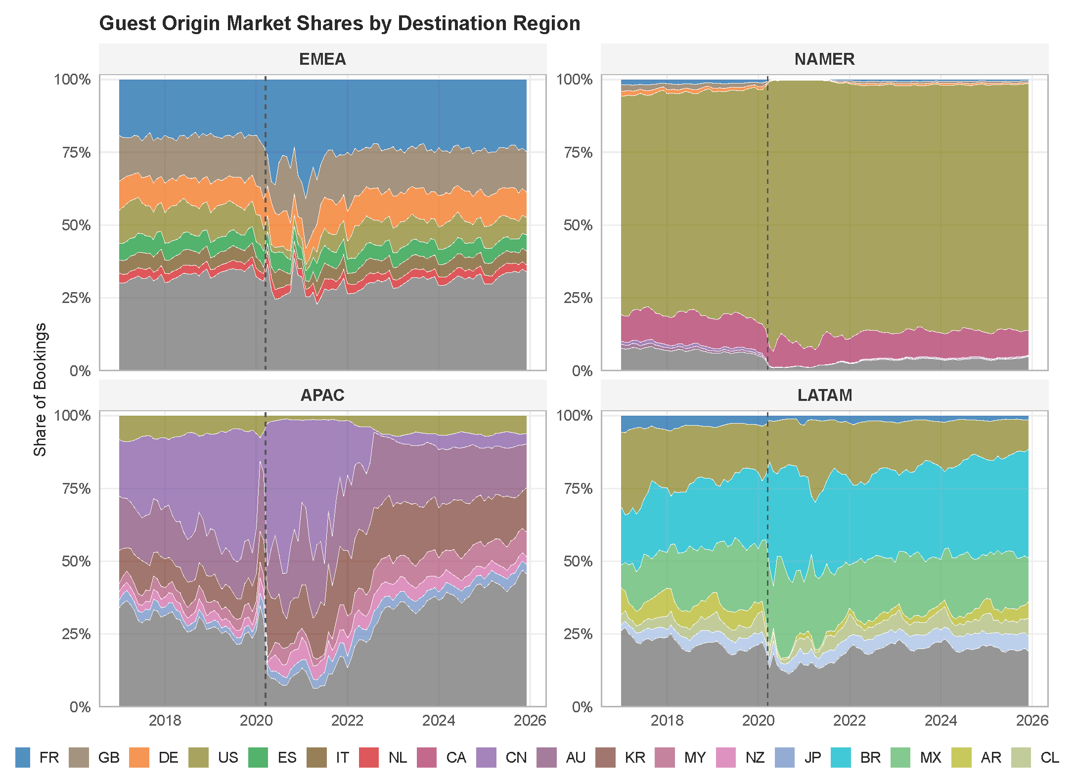
Figure 2 displays the evolution of origin market compositions over our sample period for each destination region. Several patterns emerge. First, compositions exhibit substantial temporal variation, with visible seasonal patterns (e.g., increased European-origin booking share into EMEA during summer months) and trend shifts. Second, the COVID-19 pandemic (beginning March 2020) caused dramatic compositional changes: within-region origin shares surged as long-haul booking activity collapsed. Third, the recovery from pandemic lows has been uneven across origin markets, with some shares returning to pre-pandemic levels while others show persistent deviations. Because the figure displays shares rather than counts, these movements describe changes in the booking mix; a rising share can reflect growth in that origin, contraction elsewhere, or both.
The high lag-1 autocorrelations of the raw share series (0.87–0.94 across regions; Table 2) confirm substantial persistence in compositional shares, motivating autoregressive modeling. APAC exhibits the most dramatic compositional variation, with the Chinese-origin booking share dropping from approximately 25% pre-pandemic to under 5% during restrictions, with gradual recovery thereafter. NAMER shows the least compositional variation, with U.S.-origin bookings consistently dominating at 75–90% of the total.
Both the Dirichlet likelihood and ILR transformation require strictly positive compositional components. In our data, the minimum observed share across all region-month-origin combinations is 0.8%, occurring for the “Other” category in NAMER during peak U.S.-origin months. No exact zeros appear in the data, a consequence of aggregating large booking volumes (tens of thousands of reservations per month) where even small origin markets contribute positive counts. We therefore apply no zero-replacement or smoothing procedures.

4.5. Compositional Dynamics

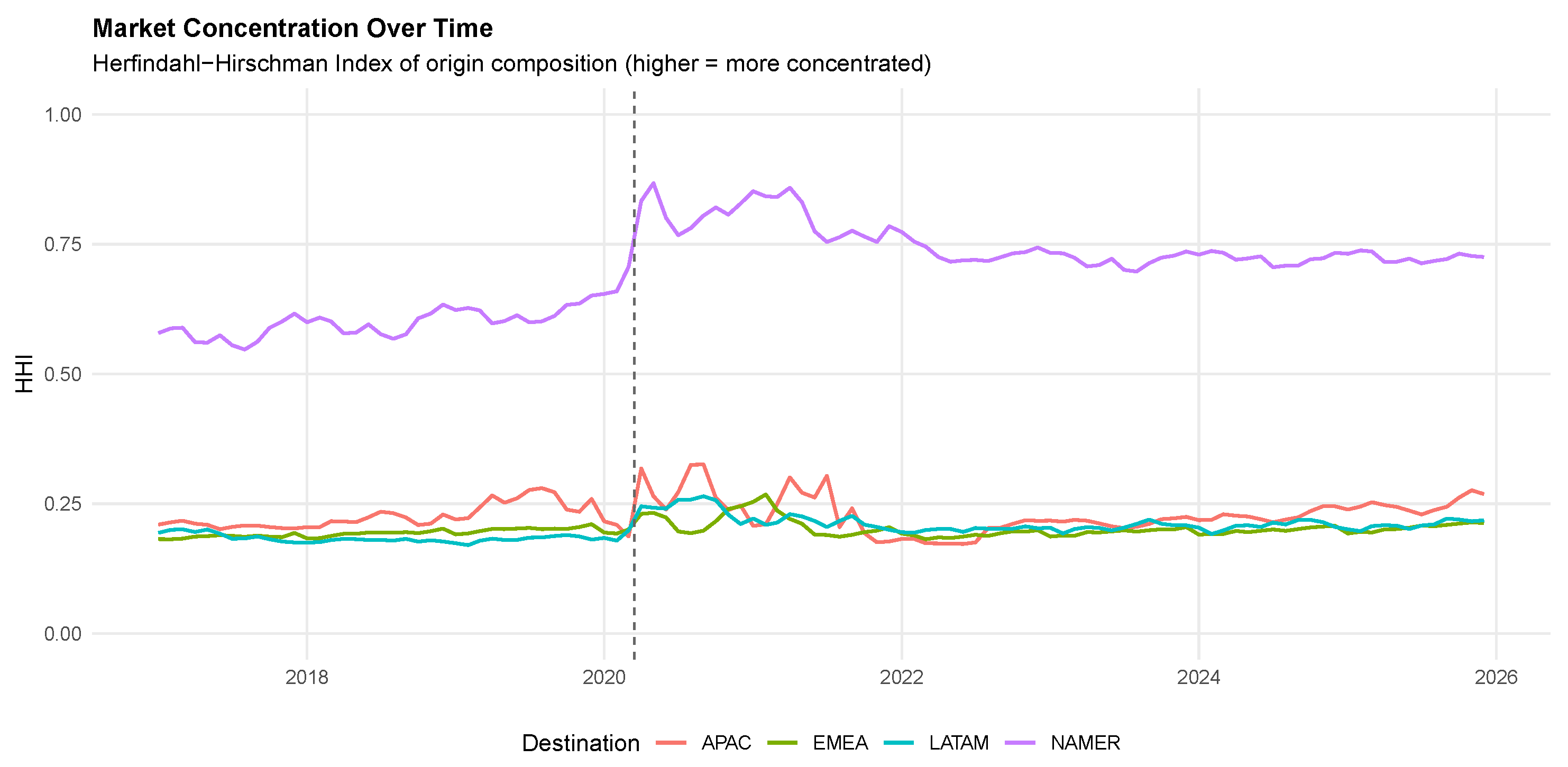
To motivate our modeling choices, we examine temporal patterns in compositional variability. Figure 3 plots the Herfindahl–Hirschman Index (HHI) of origin market concentration over time for each destination region. NAMER exhibits consistently high concentration (HHI ≈ 0.60–0.75), reflecting U.S. dominance, with a pandemic-induced spike to nearly 0.90 as Canadian cross-border travel collapsed. In contrast, EMEA, APAC, and LATAM maintain diverse origin portfolios (HHI ≈ 0.20) with only modest pandemic disruption.
Throughout, the index is computed over the eight modeled origin buckets. Because the “Other” category pools many small origins, the resulting HHI overstates concentration relative to a fully disaggregated country-level calculation: for positive shares a and b, ( a + b ) 2 > a 2 + b 2 . The index should therefore be read as concentration in the modeled composition rather than as a country-level concentration measure. This matters for the concentration-risk application discussed in Section 6.2, and we return to it in Section 6.4. The especially high concentration of NAMER is robust to this consideration, but finer comparisons among the remaining three regions should be interpreted cautiously.
This heterogeneity in market structure explains why forecast method performance varies across regions: BDARMA’s ability to model compositional dynamics provides greater value where multiple origin markets compete.
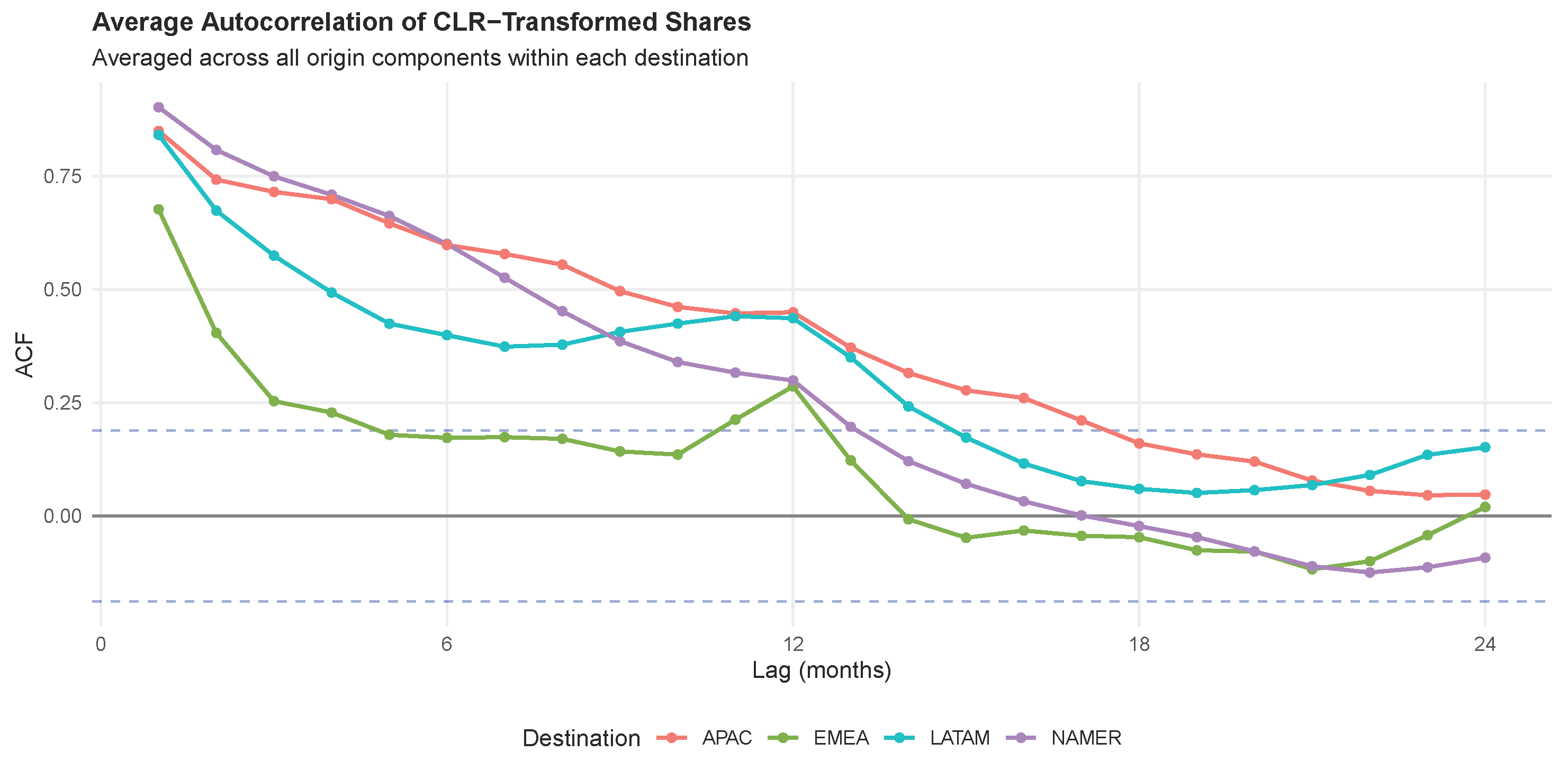
Figure 4 displays average autocorrelation functions of CLR-transformed shares by destination. All regions exhibit substantial persistence at short lags, with NAMER showing the slowest decay (lag-1 ACF ≈ 0.90) and EMEA the fastest (lag-1 ACF ≈ 0.70). APAC and LATAM display a secondary peak at lag 12, indicating seasonal patterns in composition. These autocorrelation structures motivate the AR(1) specification in our BDARMA models.
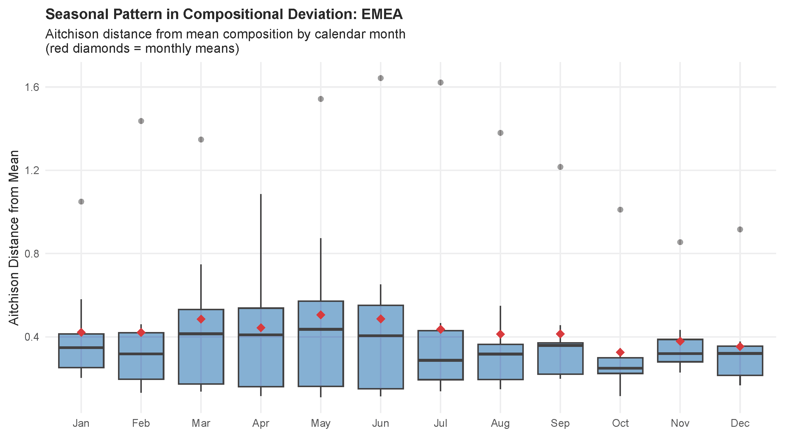
Critically, compositional variability itself exhibits seasonal patterns. Figure 5 shows boxplots of the Aitchison distance from the mean composition by calendar month for EMEA. Spring and early summer months (March–June) display substantially higher compositional dispersion than autumn months (September–October), with median Aitchison distances approximately 25% larger. This pattern reflects greater uncertainty in origin mix during shoulder seasons when booking patterns are less predictable compared to peak summer months when established seasonal flows dominate.
This empirical pattern motivates the seasonal precision specification of Equation (4): rather than assuming constant compositional volatility, we allow the Dirichlet precision parameter ϕ t to vary with Fourier seasonal terms.
Section 5.4 evaluates whether that structure earns its place.

5. Results

5.1. Model Selection

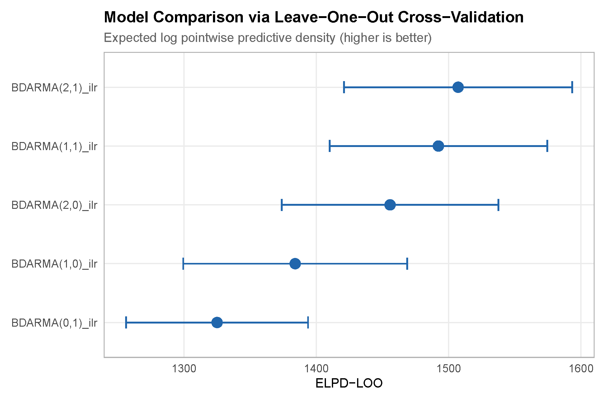
We estimate BDARMA models with varying autoregressive ( P { 0 , 1 , 2 } ) and moving average ( Q { 0 , 1 } ) orders for each destination region. All models use the ILR transformation and include Fourier terms ( K = 6 harmonics) for both the mean composition and the precision parameter. Table 3 reports LOO-CV results for EMEA, our primary analysis region. Because every specification in Table 3 includes the same seasonal-precision component, the comparison isolates dynamic order selection within the chosen model class. Section 5.4 addresses the precision specification separately, so the two model-structure questions are answered by separate comparisons rather than confounded within one.
The BDARMA(1,1) specification achieves the highest ELPD for three of four destination regions (NAMER, APAC, LATAM), while BDARMA(2,1) is preferred for EMEA, indicating that both autoregressive and moving average components contribute to forecast performance. The inclusion of the MA(1) term consistently improves model fit, suggesting that compositional shocks have effects that persist beyond what the AR dynamics alone capture. Figure 6 visualizes the LOO comparison for EMEA.

5.2. Evaluation Protocol

The out-of-sample comparison follows a fixed rolling-origin design. Forecast origins begin in January 2022 and advance in 3-month increments through April 2025, giving 14 origins per destination region. At each origin o, the information set is the monthly composition series through month o, and forecasts are produced for horizons h = 1 , , 6 , where h = 1 denotes the first calendar month after the origin. Origin categories are fixed once for the entire exercise, as described in Section 4, and are never re-selected at an origin. BDARMA orders are likewise fixed before the evaluation begins, selected by LOO-CV on the pre-evaluation window: BDARMA(2,1) for EMEA and BDARMA(1,1) for NAMER, APAC, and LATAM. At each origin, BDARMA parameters are re-estimated by MCMC on data through month o, and the ETS and SARIMA benchmarks are re-fit on the ILR-transformed series through month o with automatic order selection; naïve, seasonal naïve, and rolling-mean forecasts use only data through month o by construction. Point forecasts are posterior predictive means for BDARMA and standard point forecasts for the benchmarks, mapped back to the simplex where applicable, and accuracy is summarized by MAE averaged across the eight components and six horizons.

5.3. Forecast Accuracy

Under the protocol of Section 5.2, the 14 origins and six horizons yield 84 forecast observations per destination region.
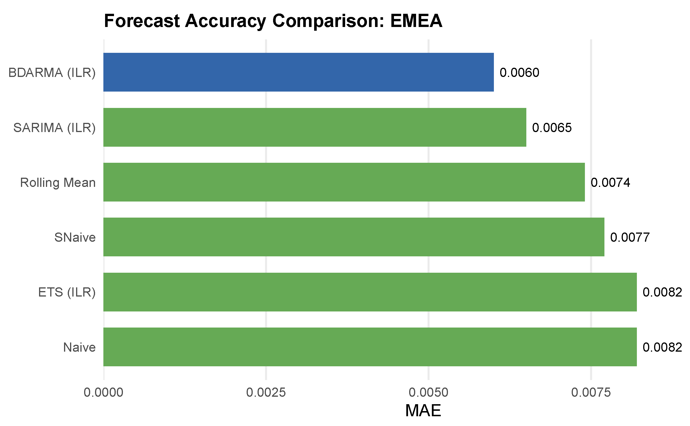
Table 4 presents the mean absolute error (MAE) for each method across destination regions. For EMEA, BDARMA achieves the lowest MAE (0.0060), representing 27% lower error than naïve forecasts (0.0082) and 8% lower than SARIMA (0.0065). Averaged across all four destinations, ETS achieves the lowest MAE (0.0086), followed closely by BDARMA (0.0089), SARIMA (0.0096), and naïve (0.0097).
The relative performance of methods varies systematically across destinations. BDARMA excels for EMEA, where compositional dynamics are rich, this region features multiple origin markets with shares between 5–25%, creating scope for autoregressive patterns to improve forecasts. For NAMER, where U.S.-origin bookings dominate at over 80%, the composition is nearly constant and all methods perform similarly. For LATAM, ETS achieves the lowest MAE (0.0075 vs. BDARMA’s 0.0108), suggesting that smooth trend dynamics dominate the autoregressive patterns that BDARMA targets. For APAC, naïve and ETS outperform BDARMA, likely because the post-pandemic recovery path for the Chinese-origin booking share is sufficiently persistent that simple extrapolation captures the dominant signal.
Figure 7 summarizes the forecast accuracy comparison for EMEA, showing BDARMA’s consistent advantage over benchmarks.
Table 5 examines forecast accuracy by horizon for EMEA. BDARMA maintains its advantage at horizons 2 and 3, with SARIMA slightly outperforming at h = 1 .
For NAMER (Table 6), where U.S.-origin bookings dominate at over 80%, all methods perform similarly. At h = 1 , ETS and naïve tie for lowest MAE (0.0009); at h = 2 , ETS leads (0.0018); at h = 3 , SARIMA leads (0.0026). BDARMA remains competitive but does not dominate in this low-variation setting.

5.4. Constant Versus Seasonal Precision

Section 3.2 introduced seasonal structure in the Dirichlet precision parameter, motivated by the descriptive evidence that compositional dispersion varies systematically across the calendar. Because every specification in Table 3 carries that structure, those comparisons cannot say what it contributes. This section addresses the question directly.
For each destination region, we refit the selected BDARMA specification with the precision equation reduced to an intercept, so that log ϕ t = γ 0 . Every other element is held fixed: the same compositions, the same Helmert ILR basis, the same K = 6 Fourier harmonics in the mean equation, the same autoregressive and moving average orders, the same priors including the precision intercept, the same 14 rolling origins and six horizons, and the same MCMC configuration. Fifty-six additional constant-precision fits are estimated, one for each of the four destination regions at each of the 14 forecast origins, and paired with the 56 seasonal-precision fits underlying Table 4. Thus, the comparison comprises 56 fits per arm, with the two arms differing only in the presence of the seasonal harmonic columns in Equation (4).
Table 7 reports the comparison. Seasonal precision lowers point forecast error in every region, by 13% in LATAM, 23% in EMEA, 34% in NAMER, and 35% in APAC. The advantage does not rest on a small number of origins: seasonal precision produces the lower error at 11 of 14 origins in EMEA and NAMER, 13 of 14 in APAC, and 10 of 14 in LATAM.
Taken together, the evidence supports seasonal precision as a component that earns its place on point accuracy across all four regions, conditional on the dynamic specification selected for each. Whether the gain extends to the predictive distribution is not addressed here, since the comparison is conducted on point accuracy alone. The result also sharpens the interpretation of Table 3: the dynamic order and the precision specification are evaluated through separate comparisons, so the LOO comparison of ARMA orders should not be read as evidence about the precision structure, and neither comparison identifies an interaction between the two.

5.5. Statistical Significance

Table 8 reports the pooled Diebold–Mariano comparisons for EMEA, treating the 14 origins and six horizons as 84 origin–horizon loss differentials. Under this pooled treatment, BDARMA has lower loss than the naïve benchmark ( p < 0.001 ), seasonal naïve ( p = 0.013 ), and ETS ( p < 0.001 ). The comparison with SARIMA is borderline ( p = 0.058 ). Because forecast horizons are nested within origins and target months overlap between adjacent origins, Appendix C reports a more conservative origin-level sensitivity analysis.
Appendix B reports the full matrix of pooled comparisons, covering all four destination regions against all five benchmarks. The pattern is regionally structured. At the unadjusted 5% level, BDARMA has lower loss than seasonal naïve in EMEA ( p = 0.013 ), NAMER ( p = 0.001 ), and APAC ( p < 0.001 ), and lower loss than the rolling mean in the same three regions. Against the naïve benchmark, the pooled evidence favors BDARMA in EMEA and LATAM ( p < 0.001 in both), shows no separation in NAMER, and favors naïve in APAC. The ETS comparison favors BDARMA in EMEA, is marginal in NAMER ( p = 0.048 ), and clearly favors ETS in LATAM, consistent with ETS attaining the lowest point accuracy for that region. Eleven of the twenty pooled comparisons reach the conventional 5% threshold.
Because the paper reports a family of twenty comparisons, Appendix B also reports Holm-adjusted p-values. Nine of the twenty pooled comparisons remain significant after adjustment; the EMEA seasonal-naïve and NAMER ETS comparisons are the two that reach the unadjusted 5% threshold but do not survive the Holm correction. Dependence within each comparison is examined separately in Appendix C, which averages the six horizons within each forecast origin and tests the resulting 14 ordered origin-level loss differentials. Under that more conservative analysis, the EMEA comparisons against naïve and ETS remain significant at p < 0.001 , and the APAC comparisons against seasonal naïve and the rolling mean remain significant. The seasonal-naïve differences for EMEA and NAMER do not remain statistically significant at the origin level and should therefore not be treated as established.

5.6. Forecast Visualization

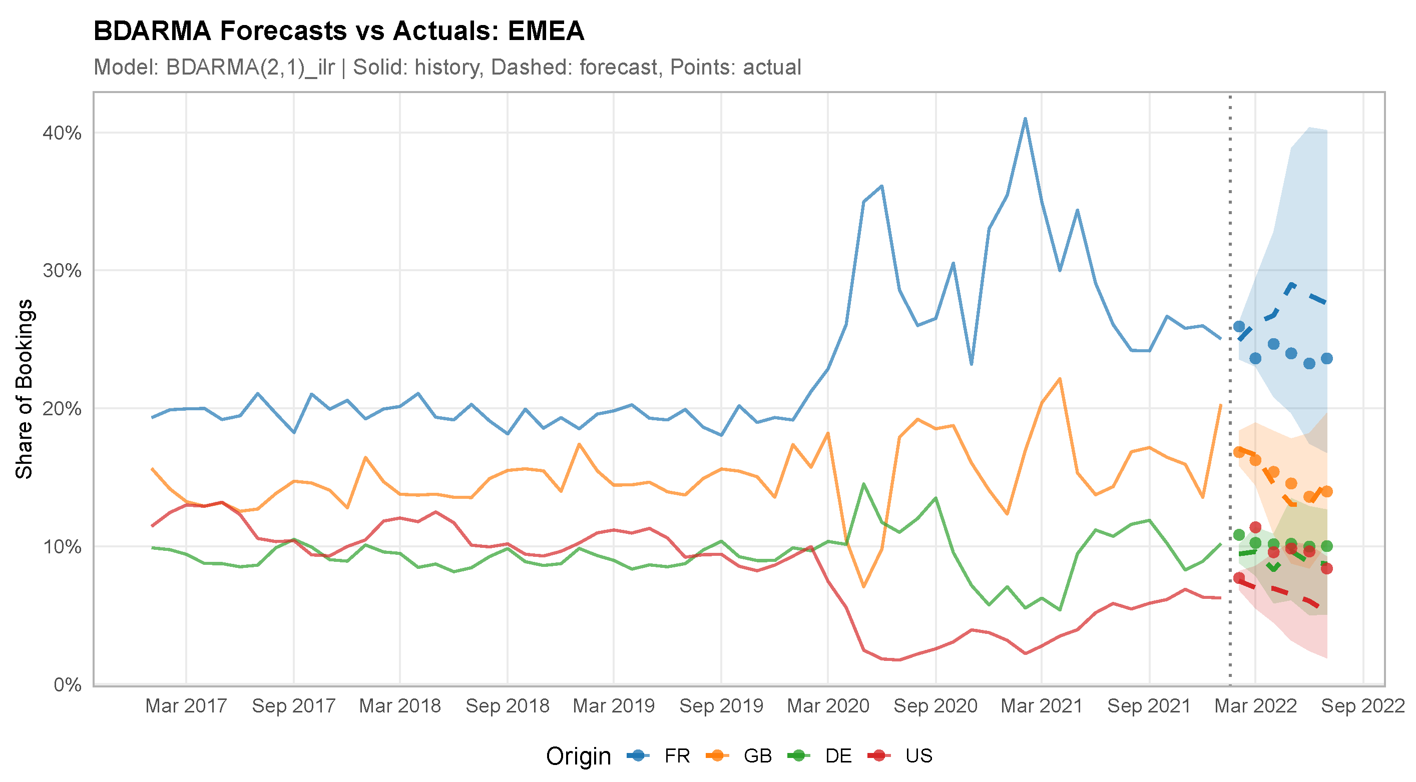
Figure 8 displays an illustrative BDARMA forecast from the first evaluation origin (January 2022) for EMEA, showing the four largest named origin markets (France, Great Britain, Germany, and the United States) with 6-month-ahead point forecasts and marginal 80% prediction intervals. The model captures the post-pandemic recovery dynamics, with shaded bands showing marginal 80% posterior predictive intervals for each plotted component, derived from the Dirichlet predictive distribution.

5.7. Component-Level Accuracy

Table 9 reports MAE by origin market component for EMEA. BDARMA achieves particularly strong accuracy for the United States component (44% improvement over naïve) and the Netherlands (50% improvement), and is second-best for Great Britain. It does not dominate component-wise: SARIMA leads for France, Italy, and Other, seasonal naïve for Great Britain, naïve for Spain, and ETS and SARIMA tie for Germany. The aggregate EMEA advantage therefore rests on large gains for a few components combined with adequate accuracy elsewhere, not on uniform superiority.

5.8. Pandemic-Era Compositional Shifts

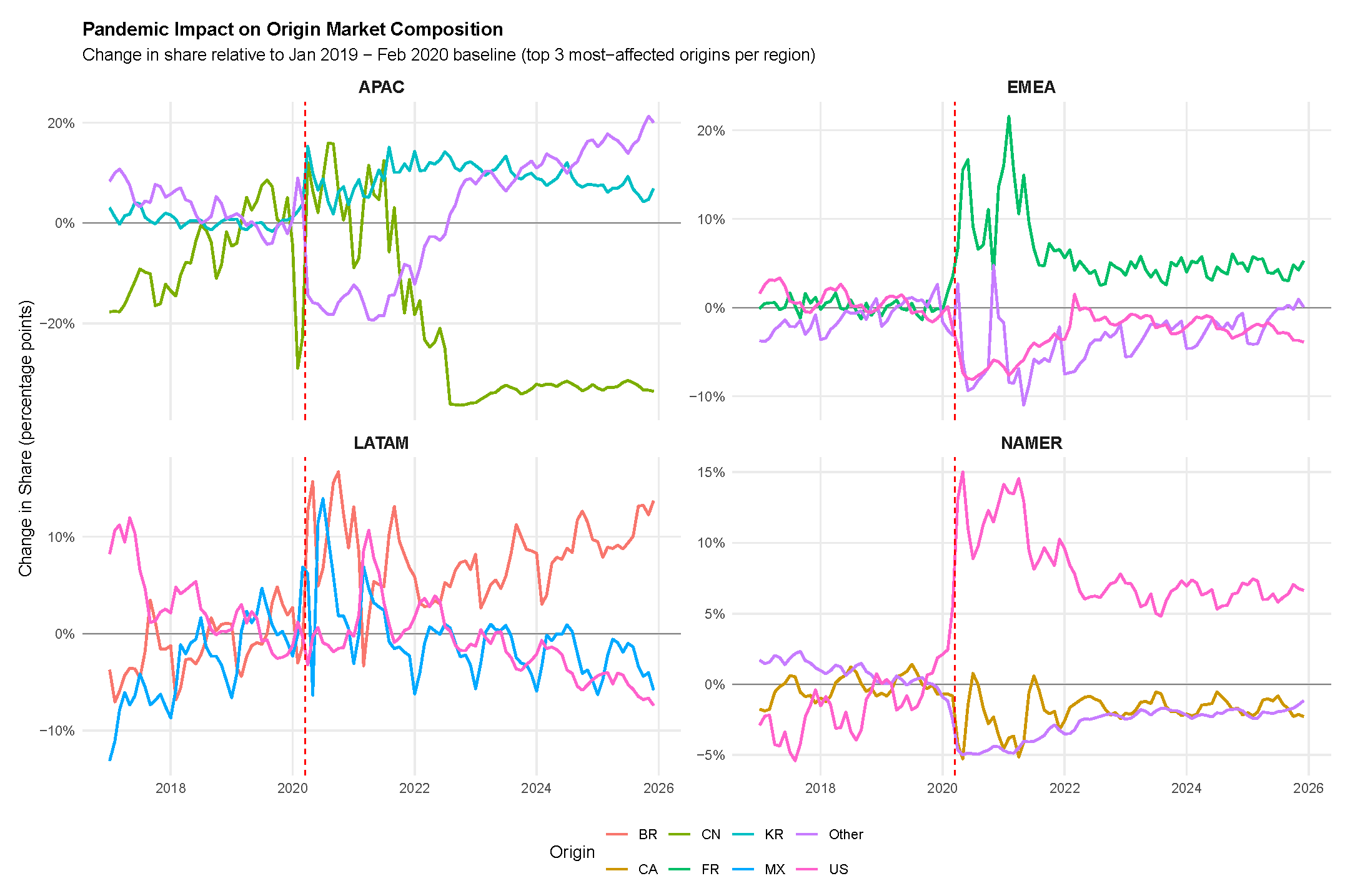
Figure 9 illustrates the pandemic’s impact on origin market compositions by plotting deviations from pre-pandemic baseline levels (January 2019–February 2020 average) for the three most-affected origin components in each destination region. The figure reveals substantial heterogeneity in how the pandemic reshaped tourism flows.
APAC experienced the most dramatic compositional shift: the Chinese-origin booking share fell by more than 20 percentage points as China maintained strict travel restrictions, while South Korean and other non-Chinese origin shares increased to partially fill the gap. EMEA saw a surge in France-origin bookings of nearly 25 percentage points during the initial lockdown period, reflecting increased within-region booking activity when international borders closed. NAMER, already dominated by U.S.-origin bookings, saw this dominance intensify by an additional 15 percentage points as Canadian cross-border travel declined. LATAM exhibited a temporary spike in Brazil-origin bookings followed by gradual normalization.
The poor performance of seasonal naïve forecasts, particularly in EMEA, NAMER, and APAC (Table 4), is consistent with the pandemic-era regime shift: using same-month-last-year values fails when the underlying compositional regime has moved. BDARMA’s autoregressive structure allows it to adapt to the new regime while still leveraging historical patterns through the Fourier seasonal terms.
The framework does not detect breaks. The models are estimated on data that already contain the pandemic shift and evaluated during the recovery, so adaptation is carried entirely by the autoregressive dynamics, and the results speak to adjustment after a break rather than to anticipating one. Specifications that identify breaks explicitly are discussed in Section 6.
Gunter et al. [35] report the same anatomy for European Airbnb occupancy: their seasonal Markov-switching autoregression forecast well during the pandemic period precisely because it detected the break while preserving seasonal structure. We return to this convergence in Section 6.

6. Discussion

6.1. Summary of Findings

Our analysis demonstrates that BDARMA models achieve the lowest forecast error for EMEA and competitive performance across other destination regions, with particular strength where multiple-origin markets exhibit rich compositional dynamics. For EMEA, BDARMA achieves 27% lower forecast error than naïve methods, with highly significant improvement ( p < 0.001 ). Averaged across all destinations, ETS slightly edges BDARMA in MAE, 0.0086 versus 0.0089, an average achieved under a protocol that permits the benchmarks to re-select their structure at every forecast origin while the BDARMA orders remain fixed. The model has lower error than seasonal naïve in EMEA, NAMER, and APAC, reflecting its ability to adapt to regime changes while still capturing underlying temporal patterns. All three comparisons reach the unadjusted 5% threshold, and the NAMER and APAC comparisons remain significant after Holm adjustment across the full family of tests. Throughout, these forecasts concern booking-month composition rather than realized stay-month arrivals, so they are best interpreted as leading indicators of market mix.
Seasonal precision earns its place in the specification. The ablation in Section 5.4 compares the selected model against an otherwise identical constant-precision version and finds lower point error in all four regions, ranging from 13% in LATAM to 35% in APAC, with seasonal precision producing the lower error at between 10 and 13 of the 14 forecast origins in each region. The mechanism is the one the descriptive evidence suggested: compositional volatility differs systematically across months, spring and early summer showing greater dispersion than autumn, and a model with constant precision has no way to represent that. The comparison establishes point accuracy rather than calibration; a full probabilistic assessment of the two specifications remains open and is identified as a near-term priority in Section 6.5.
The BDARMA(1,1) specification achieves the best in-sample fit for three of four destination regions (BDARMA(2,1) is preferred for EMEA), as measured by LOO-CV, indicating that both autoregressive and moving average components capture important features of compositional dynamics. The relative advantage of BDARMA varies systematically with the nature of compositional variation: it excels where multiple origin markets compete with shares in the 5–25% range (EMEA), performs comparably to simpler methods where one market dominates (NAMER), is outperformed by ETS in settings with smooth trend dynamics (LATAM), and is outperformed by naïve extrapolation where a single persistent recovery path dominates the signal (APAC). As shown in Section 4, the HHI concentration analysis (Figure 3) helps explain this pattern: BDARMA provides greatest value for destinations with diverse origin portfolios where compositional dynamics are meaningful.
The convergence with Gunter et al. [35] deserves emphasis. Working with occupancy levels rather than origin composition, across 43 European countries, and with a seasonal Markov-switching autoregression benchmarked against panel-data counterfactuals, they arrive at a conclusion our pandemic-era shift analysis supports from the compositional side: forecasting through the pandemic rewarded specifications that pair regime adaptation with explicit seasonal structure. Two independent routes to the same requirement make it more credible than either alone. In our framework, the adaptation is smooth, carried by the autoregressive terms. Abrupt shifts can instead be handled through gated intervention structure [49], and a Markov-switching Dirichlet ARMA in which latent regimes govern the ILR-level mean or the precision would be the direct compositional counterpart of their approach.

6.2. Implications for Destination Management

Our findings have three concrete implications for destination marketing organizations and tourism planners, corresponding to the business use cases motivating this study. We develop the first as a concise implementation workflow that links the forecast to the timing and information requirements of a decision, while treating the forecast as one input to that decision rather than as an automatic allocation rule.
Marketing budget allocation across source markets.
Consider a regional tourism-planning team responsible for source-market strategy across EMEA. At a regular planning date, the team would first generate one- to six-month forecasts of origin market composition and compare the projected changes with historical forecast error and posterior predictive uncertainty. A sufficiently large and persistent projected change would trigger managerial review rather than automatic reallocation. The team would then combine the composition forecast with campaign costs, expected incremental returns, operational constraints, and a separate forecast of aggregate booking volume before adjusting source-market allocations. The volume forecast is essential because a rising origin share may reflect growth in that origin, contraction elsewhere, or both.
The EMEA results provide the clearest empirical basis for this workflow: BDARMA reduces MAE by 27% relative to the naïve benchmark (Table 4). In NAMER, APAC, and LATAM, where simpler methods are competitive or superior, the same process should use the method with the strongest rolling-origin performance rather than assume that greater model complexity improves the decision. Predictive intervals can inform the review, but because their calibration is not formally assessed here, they should not serve as mechanical commitment thresholds. Because the forecast target is booking composition rather than stay-month arrivals, evaluation against realized visitor mix must also account for booking-to-stay lead-time drift [43].
Concentration risk monitoring.
The pandemic provided a stark illustration of the fragility that builds when origin portfolios become concentrated. As documented in Section 5.8, the Chinese-origin share of bookings into APAC fell by more than 20 percentage points within a few months. Aggregate volume forecasts alone do not reveal this form of exposure because they do not describe how demand is distributed across origin markets. BDARMA forecasts can be used alongside HHI trajectories to monitor baseline concentration exposure and identify persistent increases in dependence on a small number of source markets. This is a monitoring application rather than scenario-based stress testing, since the current model contains no explicit shock, intervention, or policy mechanism.
The caveat noted in Section 4 applies operationally as well as descriptively. The HHI is computed over the modeled origin buckets, and the aggregation of many countries into the “Other” category means that its level differs from a fully disaggregated country-level index. Its trajectory is therefore more informative for monitoring than any fixed concentration threshold.
Operational planning at the property level.
The regional forecasts estimated here are not property-specific. After extension to country- or city-level series, likely using hierarchical structure to borrow strength across sparse destinations, the same framework could support staffing, language capability, amenity, and service-design decisions. For example, a projected increase in Korean-origin share, interpreted jointly with expected total booking volume, could inform Korean-language staffing or service preparation before the travel period begins.
The seasonal-precision ablation in Section 5.4 shows that allowing compositional dispersion to vary across months improves point accuracy in every region. It does not, however, establish that the posterior predictive intervals attain their nominal coverage. The intervals should therefore be treated as indicative measures of uncertainty rather than as formal rules governing operational commitments.
These applications are most directly supported at the one- to six-month horizons evaluated in this study; longer-horizon strategic uses require separate validation. The heterogeneity in forecast performance also provides practical guidance about model complexity. BDARMA appears most useful in compositionally diverse markets where several origins hold material shares, whereas simpler methods remain competitive or superior where one origin dominates or where smooth trend dynamics carry most of the forecast signal.

6.3. Methodological Contributions

This study makes three contributions to the tourism-forecasting literature, corresponding to those stated in the abstract. We give each as a claim followed by the reason it holds, rather than resting on measured performance alone.
Contribution 1: Bayesian compositional time-series methods applied to booking-origin composition. The Dirichlet likelihood is appropriate to this problem for a structural reason rather than a convenient one: the support of the distribution and the sample space of the data coincide. Origin shares are non-negative and sum to one, which is exactly the unit simplex. Although the mean dynamics are parameterized in ILR coordinates, the observation likelihood and the posterior predictive distribution are supported directly on the simplex, so no post hoc normalization is required and every predictive draw is a valid composition. This differs from the ETS and SARIMA benchmarks used here, which fit Euclidean forecasting models to transformed coordinates and recover composition-valued forecasts only through inverse transformation.
The empirical case for this contribution rests on rolling-origin comparison against operational benchmarks, including log-ratio ETS and SARIMA with automatic order selection refitted at every origin. We report that comparison in full rather than selectively: BDARMA achieves the lowest error for EMEA and significantly outperforms naïve and ETS there, while its advantage over seasonal naïve reaches the unadjusted 5% threshold but not the Holm-adjusted threshold, and ETS attains the lowest error averaged across regions. Reporting the cases where simpler methods win is part of the point, because it identifies where compositional modeling is warranted and where it is not.
Contribution 2: Seasonal structure in the precision parameter, with its contribution isolated. The Dirichlet concentration parameter governs how tightly realizations cluster around the mean composition, and there is no principled reason to hold it constant when the dispersion of the data itself varies across the calendar. Section 4 documents that variation: the median Aitchison distance from the mean composition is roughly 25% larger in spring and early summer than in autumn. A constant-precision model must absorb that heterogeneity somewhere, and Section 5.4 measures what it costs when it cannot, finding higher point error in all four regions. The Dirichlet precision supplies a parsimonious and explicitly modeled dispersion process that the ETS and SARIMA benchmarks used here do not contain, since their predictive spread follows from the transformation and the fitted error variance rather than from a separately specified process. We note that other transformed families, logistic-normal state-space models among them, can parameterize time-varying covariance directly, so the contrast is with the specific benchmarks employed rather than with log-ratio methods in general.
Contribution 3: Booking-date indexing as a substantive choice. Indexing compositions by booking month rather than stay month makes the series observable ahead of realized arrivals, which is what allows the forecasts to inform decisions with long lead times. This is not a data-availability convenience. It changes what the forecast is for, and it introduces a linkage problem, since booking-month and stay-month compositions need not move together when lead times shift [43].

6.4. Limitations

Several limitations should be acknowledged, and we group them by what they constrain.
Data access and reproducibility. The reservation-level data underlying this study are proprietary to Airbnb and cannot be released. We mitigate it where we can: the estimation software is publicly available, the methodology is fully specified in Section 3, and the analysis code operates on any compositional series in the same layout, so the method is reproducible even where the empirics are not.
External validity. Our data capture Airbnb bookings, which represent a subset of total accommodation demand. Origin compositions may differ in both level and dynamics for hotel guests, for visitors staying with friends and relatives, and for other booking channels. Conclusions about which forecasting method suits which market structure should generalize more readily than the specific compositional trajectories we document.
Forecast horizon. We evaluate at horizons of one to six months, chosen to match the lead times of the marketing allocation decisions that motivate the study. Many tourism planning decisions operate on annual or multi-year cycles: market development strategy, language capability investment, and partnership structure among them. Longer-horizon performance is unknown, and extending the evaluation would require attention to whether the Dirichlet precision remains adequately specified as predictive uncertainty grows, since the concentration parameter governs how quickly the predictive distribution flattens.
Exogenous drivers not included. The specification estimated in this study uses lagged compositions and seasonal terms but does not include external predictors such as exchange rates, airline capacity, visa policy, fuel prices, or geopolitical indicators. Consequently, the analysis forecasts compositional dynamics without attributing them to particular external drivers or evaluating scenarios based on alternative paths of those variables. This reflects the covariate set used in the present application, not a limitation of the BDARMA framework, which can incorporate exogenous regressors through the X t covariate matrix.
Pandemic dominance of the sample. The 2017–2025 window is dominated by COVID-19 and its aftermath, and the evaluation period beginning in January 2022 falls entirely within the recovery. The advantages we document are therefore advantages under regime adaptation. Whether direct compositional modeling retains an edge over simple benchmarks in a stable tourism environment cannot be established from these results. The convergence with Gunter et al. [35], whose Markov-switching specification performed well precisely because the period rewarded regime adaptation, is consistent with this reading.
The “Other” aggregation. Consolidating markets outside the top seven into a single category simplifies estimation but pools origins whose dynamics need not resemble one another and may offset. Movement within the Other bucket is invisible to the model, and a stable Other share can conceal substantial reallocation among its constituents. This has a specific consequence for concentration-risk monitoring: the HHI reported in Section 4 is computed over the eight modeled buckets and therefore overstates concentration relative to a full country-level calculation. Since the Other category averages above 20% in several regions, the discrepancy is not negligible.
Aggregation to regions. Regional aggregation obscures within-region heterogeneity that may matter to local destination managers. A forecast for EMEA composition is of limited direct use to a manager in Lisbon.
Evaluation scope. The empirical evaluation focuses on point accuracy throughout, including the precision ablation of Section 5.4. Prediction intervals are shown illustratively rather than assessed through a calibration analysis using log scores, coverage, or Aitchison-based scoring rules. The benchmark set covers strong operational baselines but does not exhaust the space of multivariate or compositional alternatives.

6.5. Future Research

We group the extensions by what they require, since several could be undertaken immediately with the existing data and infrastructure while others need new linkage or substantial methodological development.

6.5.1. Near-Term Extensions

Probabilistic validation and calibration. The evaluation reports point accuracy throughout. A full assessment using log predictive density, interval coverage, and Aitchison-based scoring rules, applied to both the benchmark comparison and the precision ablation, would establish whether the point-accuracy gains carry over to the predictive distribution. This is the most immediate priority and requires no new data.
Exogenous predictors. Incorporating exchange rates, airline capacity, and search trends through the X t covariate matrix would improve accuracy and enable scenario analysis. The framework already accommodates this.
Broader comparator set. Extending the comparison to logistic-normal state-space models, multivariate log-ratio dynamics, and Markov-switching specifications would isolate which elements of the BDARMA specification drive its performance. The Markov-switching case is the most directly motivated: Gunter et al. [35] show that regime-switching structure carries much of the forecasting burden for pandemic-era Airbnb occupancy, and a Markov-switching Dirichlet ARMA would test whether the same holds when the target is a composition. Machine learning comparators including recurrent architectures belong here as well, though their evaluation would be more informative at the finer granularity discussed below, where the panel of series is large enough to support the parameter counts involved.

6.5.2. Longer-Term Programs

Booking-to-stay linkage. Linking booking-month compositions to check-in-month outcomes or official arrivals data would clarify when and how booking composition serves as a reliable leading indicator of realized visitor mix. This requires data integration beyond the present scope and is the most substantively important of the open questions, since it determines how the forecasts should be interpreted.
Finer geographic granularity. Country-level or city-level analysis would support targeted marketing decisions, but data sparsity at that resolution threatens the strict positivity that both the Dirichlet likelihood and the ILR transformation require. Hierarchical modeling that borrows strength across destinations would be necessary.
Combined volume and composition forecasts. Integrating compositional forecasts with aggregate volume forecasts would yield complete predictions of arrivals by origin market. Doing this coherently requires attention to how uncertainty in the two components combines.
Real-time implementation. Deploying BDARMA models in operational forecasting systems with automated updating would maximize practical value, and would require addressing the estimation cost of refitting at each origin.

7. Conclusions

This paper developed and applied Bayesian Dirichlet autoregressive moving average models to forecast the evolving composition of guest origin markets in Airbnb bookings. The target throughout is booking-month composition, so the results should be read as forecasts of platform booking demand and of the booking pipeline, not as direct forecasts of stay-month arrivals. Our analysis of 108 months of reservations across four major destination regions demonstrates that BDARMA achieves 27% lower forecast error than naïve methods for EMEA, with strong evidence under both the pooled and origin-level comparisons ( p < 0.001 ).
BDARMA also has lower error than seasonal naïve in EMEA, NAMER, and APAC. The pooled comparisons provide Holm-adjusted evidence in NAMER and APAC, while the more conservative origin-level sensitivity analysis retains clear statistical evidence only for APAC. Averaged across destinations, ETS attains the lowest error, with BDARMA close behind; BDARMA’s advantage is concentrated in compositionally diverse markets where multiple origin markets compete for shares in the 5–25% range.
The COVID-19 pandemic caused dramatic compositional shifts, most notably the collapse of the Chinese-origin booking share into APAC and the surge in within-region bookings across all destinations, with recovery trajectories that varied markedly across regions. Our models capture these dynamics through autoregressive and moving average terms while the Dirichlet likelihood ensures forecasts remain valid probability distributions.
Allowing seasonal variation in the precision parameter improves point accuracy in every destination region, by between 13% and 35% relative to an otherwise identical constant-precision specification, conditional on each region’s selected autoregressive and moving-average structure. The comparison concerns point accuracy; the corresponding effect on interval calibration is not established here.
The methodological contribution lies in bringing recent advances in Bayesian compositional time series to tourism forecasting with an explicit focus on booking-date origin shares. The empirical contribution documents substantial heterogeneity in how origin market compositions evolved during and after the pandemic, with direct implications for destination marketing strategy.
We opened this paper with three decisions that require knowing not just how many visitors may eventually arrive, but what the booking pipeline suggests about where they will come from: marketing budget allocation across source markets, concentration risk monitoring, and operational planning at the property level. These decisions share a common structure. They must be made months in advance, they are difficult to reverse once committed, and they depend critically on the composition of demand rather than its aggregate volume. A destination that watched its Chinese-origin booking share grow from 15% to 25% over three years before the pandemic was accumulating fragility that no aggregate volume forecast would have revealed. A DMO setting its Q3 campaign budget in January needs a distributional view of where its booking demand is coming from, not just how much there is. The BDARMA framework, with its coherent simplex-valued forecasts and uncertainty quantification, is designed precisely for this class of decision. As tourism markets continue to evolve in response to changing travel preferences, economic conditions, and potential future disruptions, the ability to forecast demand composition in forward-looking booking data will remain a practical imperative for destination stakeholders.


Funding

This research received no external funding.

Data Availability Statement

The reservation-level data underlying this study are proprietary to Airbnb, Inc. and cannot be shared, which prevents independent replication of the specific numerical results reported here. The darma R package (version 0.1.0) used for estimation is publicly available at https://github.com/harrisonekatz/darma (accessed on 13 August 2026). The code operates on any compositional time series supplied in the same layout, so the methodology is reproducible independently of the proprietary data.

Conflicts of Interest

The author is an employee of Airbnb, Inc., and the study uses Airbnb’s internal reservation data. The author declares no other competing interests.

Appendix A. Technical Details

Appendix A.1. Innovation Structure

The moving-average innovations in Equation (3) are the raw ILR-scale residuals ϵ t = ILR ( y t ) η t . Under the Dirichlet likelihood, these do not have conditional mean zero, because E [ log Y c ] log E [ Y c ] for Dirichlet-distributed random variables. Specifically, if Y Dirichlet ( ϕ μ ) , then
E [ log Y c ] = ψ ( ϕ μ c ) ψ ( ϕ ) ,
where ψ ( · ) denotes the digamma function, so that E [ ϵ t μ t , ϕ t ] = V E [ log Y t ] log μ t 0 in general. The bias is a smooth function of ( μ t , ϕ t ) and shrinks as the precision grows.
Centering would replace ϵ t with
ϵ ~ t = ILR ( y t ) E [ ILR ( Y t ) μ t , ϕ t ] ,
which restores E [ ϵ ~ t μ t , ϕ t ] = 0 [50]. The conditional expectation is obtained by applying the ILR contrast matrix to the vector of component-wise expectations ( ψ ( ϕ t μ t , 1 ) ψ ( ϕ t ) , , ψ ( ϕ t μ t , C ) ψ ( ϕ t ) ) , and the centered formulation is implemented in the same software as an alternative specification.

Appendix A.2. Diebold–Mariano Test Implementation

Let L m ( o , h ) denote the loss of method m at forecast origin o and horizon h, computed as the mean absolute error averaged across the C = 8 compositional components:
L m ( o , h ) = 1 C c = 1 C y ^ o , h , c ( m ) y o , h , c .
The loss differential between BDARMA and a benchmark is d ( o , h ) = L BDARMA ( o , h ) L benchmark ( o , h ) , so negative values favor BDARMA. The Diebold–Mariano statistic is
DM = k · d ¯ γ ^ 0 / n ,
where d ¯ = n 1 d ( o , h ) , γ ^ 0 = n 1 ( d ( o , h ) d ¯ ) 2 , and k = ( n + 1 2 h + h ( h 1 ) / n ) / n is the finite-sample correction of Harvey et al. [51]. With n = 84 forecast observations (14 origins × 6 horizons) and h = 1 , the correction reduces to k = ( n 1 ) / n . Given the moderate sample size, we report p-values from the t n 1 distribution rather than the asymptotic normal [47].

Appendix B. Complete Diebold–Mariano Comparisons

Table A1 reports the full set of Diebold–Mariano comparisons across all four destination regions and all five benchmarks, extending the EMEA results of Table 8. The one-sided alternative in every case is that BDARMA has lower loss, so negative statistics favor BDARMA.
Table A1. Diebold–Mariano comparisons: All destination regions and benchmarks.
RegionBenchmarkBDARMABench.MeanDMpHolm
MAEMAEDiff.Stat. p
EMEANaïve0.00600.0082 0.00221 5.93 <0.001<0.001
Seasonal naïve0.00600.0077 0.00165 2.26 0.0130.147
Rolling mean0.00600.0074 0.00134 3.49 <0.0010.006
ETS0.00600.0082 0.00220 7.34 <0.001<0.001
SARIMA0.00600.0065 0.00047 1.59 0.0580.523
NAMERNaïve0.00230.0025 0.00026 1.22 0.1120.897
Seasonal naïve0.00230.0035 0.00120 3.26 0.0010.010
Rolling mean0.00230.0030 0.00074 3.47 <0.0010.006
ETS0.00230.0027 0.00041 1.68 0.0480.480
SARIMA0.00230.0022 0.00004 0.17 0.5681.000
APACNaïve0.01630.0144 0.00198 2.01 0.9761.000
Seasonal naïve0.01630.0323 0.01596 8.02 <0.001<0.001
Rolling mean0.01630.0232 0.00686 6.44 <0.001<0.001
ETS0.01630.0160 0.00036 0.37 0.6431.000
SARIMA0.01630.0188 0.00245 2.81 0.0030.037
LATAMNaïve0.01080.0136 0.00278 4.10 <0.0010.001
Seasonal naïve0.01080.0110 0.00024 0.37 0.3541.000
Rolling mean0.01080.0110 0.00024 0.36 0.3621.000
ETS0.01080.0075 0.00325 6.98 1.0001.000
SARIMA0.01080.0107 0.00010 0.14 0.5551.000
Note: One-sided tests of the alternative that BDARMA has lower loss; negative mean differences and negative statistics favor BDARMA. Loss is component-wise MAE averaged across the eight compositional components at each of 14 forecast origins and six horizons, giving n = 84 observations per comparison. Statistics use the finite-sample correction of Harvey et al. [51] and are referred to a t 83 distribution; see Appendix A. The Holm column adjusts the one-sided p-values across the complete family of 20 comparisons. Eleven comparisons reach the 5% level unadjusted and nine after adjustment.

Appendix C. Origin-Level Sensitivity of the Diebold–Mariano Comparisons

The comparisons in Appendix B pool all 14 × 6 = 84 origin-horizon cells and estimate the variance of the loss differential from its contemporaneous autocovariance. That treatment does not account for the nesting of six horizons within each forecast origin, for target months that overlap between adjacent origins, or for the absence of a single natural time ordering across the pooled cells. The effective number of independent observations is closer to the 14 forecast origins than to 84.
Table A2 reports a sensitivity analysis under a more conservative treatment of that dependence. Loss differentials are averaged across the six horizons within each forecast origin, yielding 14 ordered paired differences per comparison. The mean is then tested with a Newey–West HAC standard error at lag one, without prewhitening and with the finite-sample adjustment, referred to a t 13 distribution.
Table A2. Origin-level sensitivity analysis of the Diebold–Mariano comparisons.
RegionBenchmarkMean Diff.HAC SEtpPooled p
EMEANaïve 0.00221 0.00047 4.75 <0.001<0.001
Seasonal naïve 0.00165 0.00201 0.82 0.2130.013
Rolling mean 0.00134 0.00085 1.58 0.069<0.001
ETS 0.00220 0.00035 6.27 <0.001<0.001
SARIMA 0.00047 0.00041 1.15 0.1350.058
NAMERNaïve 0.00026 0.00032 0.82 0.2130.112
Seasonal naïve 0.00120 0.00091 1.32 0.1050.001
Rolling mean 0.00074 0.00043 1.73 0.054<0.001
ETS 0.00041 0.00040 1.03 0.1610.048
SARIMA 0.00004 0.00037 0.11 0.5440.568
APACNaïve 0.00198 0.00227 0.87 0.8000.976
Seasonal naïve 0.01596 0.00565 2.83 0.007<0.001
Rolling mean 0.00686 0.00288 2.38 0.017<0.001
ETS 0.00036 0.00194 0.18 0.5720.643
SARIMA 0.00245 0.00178 1.38 0.0950.003
LATAMNaïve 0.00278 0.00111 2.50 0.013<0.001
Seasonal naïve 0.00024 0.00134 0.18 0.4320.354
Rolling mean 0.00024 0.00127 0.19 0.4250.362
ETS 0.00325 0.00091 3.56 0.9981.000
SARIMA 0.00010 0.00152 0.06 0.5250.555
Note: Loss differentials are averaged across the six horizons within each of the 14 forecast origins, giving n = 14 ordered paired observations per comparison. Standard errors use a Newey–West estimator at lag one without prewhitening and with finite-sample adjustment; p-values are one-sided against a t 13 reference. The final column repeats the pooled p-value from Table A1 for comparison. Negative differences favor BDARMA.
The two treatments agree qualitatively in 14 of the 20 comparisons at the 5% level. All six disagreements run in the same direction: a comparison significant under pooling is not significant under the origin-level treatment, which is the expected consequence of reducing the effective sample size from 84 to 14. The results that the paper’s conclusions rest on survive: BDARMA against naïve and against ETS in EMEA remain significant at p < 0.001 , and the APAC comparisons against seasonal naïve and rolling mean remain significant. The EMEA comparison against seasonal naïve is the most affected, moving from p = 0.013 to p = 0.213 , and should be regarded as suggestive rather than established. We report the pooled results in the main text because they follow the conventional Diebold–Mariano application to a rolling-origin design, and we report this analysis alongside them because the pooled degrees of freedom are optimistic.

References

  1. Song, H.; Qiu, R.T.R.; Park, J. A review of research on tourism demand forecasting: Launching the Annals of Tourism Research curated collection on tourism demand forecasting. Ann. Tour. Res. 2019, 75, 338–362. [Google Scholar] [CrossRef] [Scilit]
  2. Witt, S.F.; Witt, C.A. Forecasting tourism demand: A review of empirical research. Int. J. Forecast. 1995, 11, 447–475. [Google Scholar] [CrossRef] [Scilit]
  3. Song, H.; Li, G. Tourism demand modelling and forecasting: A review of recent research. Tour. Manag. 2008, 29, 203–220. [Google Scholar] [CrossRef] [Scilit]
  4. Assaf, A.G.; Li, G.; Song, H.; Tsionas, M.G. Modeling and forecasting regional tourism demand using the Bayesian global vector autoregressive (BGVAR) model. J. Travel Res. 2019, 58, 383–397. [Google Scholar] [CrossRef] [Scilit]
  5. Jiao, E.X.; Chen, J.L. Tourism forecasting: A review of methodological developments over the last decade. Tour. Econ. 2019, 25, 469–492. [Google Scholar] [CrossRef] [Scilit]
  6. Wu, D.C.; Song, H.; Shen, S. New developments in tourism and hotel demand modeling and forecasting. Int. J. Contemp. Hosp. Manag. 2017, 29, 507–529. [Google Scholar] [CrossRef] [Scilit]
  7. Wu, D.C.; Li, G.; Song, H. Economic analysis of tourism consumption dynamics: A time-varying parameter demand system approach. Ann. Tour. Res. 2012, 39, 667–685. [Google Scholar] [CrossRef] [Scilit]
  8. Divisekera, S. A model of demand for international tourism. Ann. Tour. Res. 2003, 30, 31–49. [Google Scholar] [CrossRef] [Scilit]
  9. Gössling, S.; Scott, D.; Hall, C.M. Pandemics, tourism and global change: A rapid assessment of COVID-19. J. Sustain. Tour. 2021, 29, 1–20. [Google Scholar] [CrossRef] [Scilit]
  10. Sigala, M. Tourism and COVID-19: Impacts and implications for advancing and resetting industry and research. J. Bus. Res. 2020, 117, 312–321. [Google Scholar] [CrossRef] [Scilit] [PubMed]
  11. Aitchison, J. The Statistical Analysis of Compositional Data; Chapman and Hall: London, UK, 1986. [Google Scholar] [CrossRef] [Scilit]
  12. Pawlowsky-Glahn, V.; Egozcue, J.J.; Tolosana-Delgado, R. Modeling and Analysis of Compositional Data; Wiley: Chichester, UK, 2015. [Google Scholar] [CrossRef] [Scilit]
  13. Aitchison, J. The statistical analysis of compositional data. J. R. Stat. Soc. Ser. B 1982, 44, 139–177. [Google Scholar] [CrossRef] [Scilit]
  14. Greenacre, M. Compositional data analysis. Annu. Rev. Stat. Its Appl. 2021, 8, 271–299. [Google Scholar] [CrossRef] [Scilit]
  15. Katz, H.; Brusch, K.T.; Weiss, R.E. A Bayesian Dirichlet auto-regressive moving average model for forecasting lead times. Int. J. Forecast. 2024, 40, 1556–1567. [Google Scholar] [CrossRef] [Scilit]
  16. Song, H.; Qiu, R.T.R.; Park, J. Progress in tourism demand research: Theory and empirics. Tour. Manag. 2023, 94, 104655. [Google Scholar] [CrossRef] [Scilit]
  17. Song, H.; Li, G.; Witt, S.F.; Athanasopoulos, G. Forecasting tourist arrivals using time-varying parameter structural time series models. Int. J. Forecast. 2011, 27, 855–869. [Google Scholar] [CrossRef] [Scilit]
  18. Li, G.; Song, H.; Witt, S.F. Time varying parameter and fixed parameter linear AIDS: An application to tourism demand forecasting. Int. J. Forecast. 2006, 22, 57–71. [Google Scholar] [CrossRef] [Scilit]
  19. Athanasopoulos, G.; Hyndman, R.J.; Song, H.; Wu, D.C. The tourism forecasting competition. Int. J. Forecast. 2011, 27, 822–844. [Google Scholar] [CrossRef] [Scilit]
  20. Song, H.; Liu, A.; Li, G.; Liu, X. Bayesian bootstrap aggregation for tourism demand forecasting. Int. J. Tour. Res. 2021, 23, 914–927. [Google Scholar] [CrossRef] [Scilit]
  21. Liu, X.; Liu, A.; Chen, J.L.; Li, G. Impact of decomposition on time series bagging forecasting performance. Tour. Manag. 2023, 97, 104725. [Google Scholar] [CrossRef] [Scilit]
  22. Sun, S.; Wei, Y.; Tsui, K.L.; Wang, S. Forecasting tourist arrivals with machine learning and internet search index. Tour. Manag. 2019, 70, 1–10. [Google Scholar] [CrossRef] [Scilit]
  23. Li, H.; Hu, M.; Li, G. Forecasting Tourism Demand with Multisource Big Data. Ann. Tour. Res. 2020, 83, 102912. [Google Scholar] [CrossRef] [Scilit]
  24. Li, X.; Law, R.; Xie, G.; Wang, S. Review of tourism forecasting research with internet data. Tour. Manag. 2021, 83, 104245. [Google Scholar] [CrossRef] [Scilit]
  25. Hu, M.; Li, H.; Song, H.; Li, X.; Law, R. Tourism demand forecasting using tourist-generated online review data. Tour. Manag. 2022, 90, 104490. [Google Scholar] [CrossRef] [Scilit]
  26. Wu, J.; Li, M.; Zhao, E.; Sun, S.; Wang, S. Can multi-source heterogeneous data improve the forecasting performance of tourist arrivals amid COVID-19? Mixed-data sampling approach. Tour. Manag. 2023, 98, 104759. [Google Scholar] [CrossRef] [Scilit] [PubMed]
  27. Mikulić, J.; Baumgärtner, R.M. Google trends and Baidu index data in tourism demand forecasting: A critical assessment of recent applications. Tour. Manag. 2025, 110, 105164. [Google Scholar] [CrossRef] [Scilit]
  28. Kynčlová, P.; Filzmoser, P.; Hron, K. Modeling compositional time series with vector autoregressive models. J. Forecast. 2015, 34, 303–314. [Google Scholar] [CrossRef] [Scilit]
  29. Egozcue, J.J.; Pawlowsky-Glahn, V.; Mateu-Figueras, G.; Barcelo-Vidal, C. Isometric logratio transformations for compositional data analysis. Math. Geol. 2003, 35, 279–300. [Google Scholar] [CrossRef] [Scilit]
  30. Grunwald, G.K.; Raftery, A.E.; Guttorp, P. Time series of continuous proportions. J. R. Stat. Soc. Ser. B 1993, 55, 103–116. [Google Scholar] [CrossRef] [Scilit]
  31. Zheng, T.; Chen, R. Dirichlet ARMA Models for Compositional Time Series. J. Multivar. Anal. 2017, 158, 31–46. [Google Scholar] [CrossRef] [Scilit]
  32. Gunter, U.; Önder, I. Determinants of Airbnb demand in Vienna and their implications for the traditional accommodation industry. Tour. Econ. 2018, 24, 270–293. [Google Scholar] [CrossRef] [Scilit]
  33. Gunter, U.; Önder, I.; Zekan, B. Modeling Airbnb demand to New York City while employing spatial panel data at the listing level. Tour. Manag. 2020, 77, 104000. [Google Scholar] [CrossRef] [Scilit]
  34. Milone, F.L.; Gunter, U.; Zekan, B. The pricing of European Airbnb listings during the pandemic: A difference-in-differences approach employing COVID-19 response strategies as a continuous treatment. Tour. Manag. 2023, 97, 104738. [Google Scholar] [CrossRef] [Scilit] [PubMed]
  35. Gunter, U.; Zekan, B.; Milone, F.L. Modelling and forecasting European Airbnb occupancy during the pandemic: The specific merits of panel-data and Markov-switching models. Tour. Econ. 2025, 31, 695–713. [Google Scholar] [CrossRef] [Scilit]
  36. Song, H.; Li, G.; Cai, Y. Tourism forecasting competition in the time of COVID-19: An assessment of ex ante forecasts. Ann. Tour. Res. 2022, 96, 103445. [Google Scholar] [CrossRef] [Scilit] [PubMed]
  37. Zervas, G.; Proserpio, D.; Byers, J.W. The rise of the sharing economy: Estimating the impact of Airbnb on the hotel industry. J. Mark. Res. 2017, 54, 687–705. [Google Scholar] [CrossRef] [Scilit]
  38. Sainaghi, R.; Chica-Olmo, J. The effects of location before and during COVID-19: Impacts on revenue of Airbnb listings in Milan (Italy). Ann. Tour. Res. 2022, 96, 103464. [Google Scholar] [CrossRef] [Scilit] [PubMed]
  39. Guttentag, D. Airbnb: Disruptive innovation and the rise of an informal tourism accommodation sector. Curr. Issues Tour. 2015, 18, 1192–1217. [Google Scholar] [CrossRef] [Scilit]
  40. Dolnicar, S. A review of research into paid online peer-to-peer accommodation: Launching the Annals of Tourism Research curated collection on peer-to-peer accommodation. Ann. Tour. Res. 2019, 75, 248–264. [Google Scholar] [CrossRef] [Scilit]
  41. Hall, C.M.; Prayag, G.; Safonov, A.; Coles, T.; Gössling, S.; Naderi Koupaei, S. Airbnb and the sharing economy. Curr. Issues Tour. 2022, 25, 3057–3067. [Google Scholar] [CrossRef] [Scilit]
  42. Nieuwland, S.; Van Melik, R. Regulating Airbnb: How cities deal with perceived negative externalities of short-term rentals. Curr. Issues Tour. 2020, 23, 811–825. [Google Scholar] [CrossRef] [Scilit]
  43. Katz, H.; Savage, E.; Coles, P. Lead times in flux: Analyzing Airbnb booking dynamics during global upheavals (2018–2022). Ann. Tour. Res. Empir. Insights 2025, 6, 100185. [Google Scholar] [CrossRef] [Scilit]
  44. Carpenter, B.; Gelman, A.; Hoffman, M.D.; Lee, D.; Goodrich, B.; Betancourt, M.; Brubaker, M.; Guo, J.; Li, P.; Riddell, A. Stan: A probabilistic programming language. J. Stat. Softw. 2017, 76, 1–32. [Google Scholar] [CrossRef] [Scilit] [PubMed]
  45. Vehtari, A.; Gelman, A.; Simpson, D.; Carpenter, B.; Bürkner, P.C. Rank-normalization, folding, and localization: An improved R ^ for assessing convergence of MCMC. Bayesian Anal. 2021, 16, 667–718. [Google Scholar] [CrossRef] [Scilit]
  46. Vehtari, A.; Gelman, A.; Gabry, J. Practical Bayesian model evaluation using leave-one-out cross-validation and WAIC. Stat. Comput. 2017, 27, 1413–1432. [Google Scholar] [CrossRef] [Scilit]
  47. Diebold, F.X.; Mariano, R.S. Comparing predictive accuracy. J. Bus. Econ. Stat. 1995, 13, 253–263. [Google Scholar] [CrossRef] [Scilit]
  48. Airbnb, Inc. Airbnb Q4 2024 Shareholder Letter; Investor Relations; Airbnb, Inc.: San Francisco, CA, USA, 2025. [Google Scholar]
  49. Katz, H. Directional-Shift Dirichlet ARMA Models for Compositional Time Series with Structural Break Intervention. arXiv 2026, arXiv:2601.16821. [Google Scholar] [CrossRef] [Scilit]
  50. Katz, H. Centered-Innovation MA for Bayesian Dirichlet ARMA: Theoretical Equivalence and an Application to Bank-Asset Shares. arXiv 2026, arXiv:2510.18903. [Google Scholar] [CrossRef] [Scilit]
  51. Harvey, D.; Leybourne, S.; Newbold, P. Testing the equality of prediction mean squared errors. Int. J. Forecast. 1997, 13, 281–291. [Google Scholar] [CrossRef] [Scilit]
Figure 1. Analytical workflow. Compositions are constructed on the booking-date axis, mapped to R C 1 by a fixed isometric log-ratio basis, and modeled with VARMA dynamics on the mean alongside a separate seasonal equation for the Dirichlet precision. The model is re-estimated at each of 14 forecast origins and evaluated against five operational benchmarks.
Forecasting 08 00074 g001
Figure 2. Guest origin market shares by destination region, January 2017–December 2025. Stacked area charts show the compositional evolution of the top seven origin markets plus “Other” for each destination. The vertical dashed line indicates March 2020 (onset of COVID-19 pandemic). Note the dramatic compositional shifts during 2020–2021, particularly the collapse of the Chinese-origin booking share into APAC and the surge in within-region bookings across all destinations.
Forecasting 08 00074 g002
Figure 3. Market concentration over time by destination region. The Herfindahl–Hirschman Index (HHI), computed over the eight modeled origin buckets, measures origin market concentration, with higher values indicating dominance by fewer markets. NAMER exhibits consistently high concentration due to U.S. dominance, while EMEA maintains diverse origin portfolios. The vertical dashed line indicates March 2020.
Forecasting 08 00074 g003
Figure 4. Average autocorrelation of CLR-transformed origin shares by destination region. All regions show substantial persistence, with NAMER exhibiting the slowest decay. The seasonal bump at lag 12 for APAC and LATAM motivates including Fourier terms for seasonality.
Forecasting 08 00074 g004
Figure 5. Seasonal pattern in compositional deviation for EMEA. Boxplots show Aitchison distance from mean composition by calendar month; red diamonds indicate monthly means. Spring and early summer months exhibit greater compositional dispersion than autumn, motivating the seasonal precision specification in our BDARMA models.
Forecasting 08 00074 g005
Figure 6. Model comparison via leave-one-out cross-validation for EMEA. Blue circles indicate posterior mean ELPD; error bars show ± 2 standard errors. The BDARMA(2,1) specification achieves the highest expected log predictive density.
Forecasting 08 00074 g006
Figure 7. Forecast accuracy comparison for EMEA destination. BDARMA achieves the lowest mean absolute error (0.0060), followed by SARIMA (0.0065), Rolling Mean (0.0074), and Seasonal Naïve (0.0077), with ETS and Naïve tied at 0.0082.
Forecasting 08 00074 g007
Figure 8. Illustrative BDARMA(2,1) forecast from the first evaluation origin (January 2022) for EMEA, showing the four largest named origin markets (France, Great Britain, Germany, United States). Solid lines show historical compositions; dashed lines show 6-month-ahead point forecasts; shaded regions indicate marginal 80% posterior predictive intervals for each component; points show realized values.
Forecasting 08 00074 g008
Figure 9. Pandemic impact on origin market composition by destination region. Lines show changes in market share relative to the January 2019–February 2020 baseline for the three most-affected origin components in each region. The vertical dashed red line indicates March 2020 (WHO pandemic declaration). Note the heterogeneous responses in booking composition: APAC saw the Chinese-origin share fall by more than 20 percentage points; EMEA experienced a France-origin surge of 25 percentage points; NAMER’s U.S.-origin dominance intensified; LATAM showed temporary Brazil-origin gains followed by normalization.
Forecasting 08 00074 g009
Table 1. Forecasting approaches in tourism demand and their treatment of compositional structure.
Method FamilyTypical ApplicationCompositional HandlingCentral Finding
Econometric demand models [2,3]Arrivals, overnights, expenditure by originNone; scalar outcomes modeled separatelyMacroeconomic drivers explain demand levels but require exogenous forecasts
Time-varying parameter and structural change [17,18]Arrivals under evolving relationshipsNoneParameter instability is material; adaptive formulations improve accuracy
Almost-ideal demand systems [7,18]Budget shares across products or destinationsShares modeled jointly; simplex not enforced by constructionExpenditure allocation responds to relative prices; linear forms admit incoherent shares
Univariate and automated benchmarks [19,20,21]Arrivals; competition settingsNot applicableSimple methods are difficult to beat; combination and stabilization help
Search and multisource big data [22,23,24,25,26]Short-horizon arrivals, disrupted periodsNoneDigital traces improve short-horizon accuracy; sensitive to query design [27]
Log-ratio time series [28,29]Compositional series outside tourismSimplex mapped to Euclidean space; coherence by transformationStandard multivariate machinery applies; interpretation and near-zero shares are costly
Dirichlet time series [15,30,31]Compositional series; lead times, asset sharesDistribution supported on the simplex; coherence by constructionDispersion is a modeled parameter; full predictive distributions available
Platform-data forecasting [32,33,34,35]Airbnb occupancy, demand volume, priceNone; scalar targetsPlatform demand is predictable; regime-switching structure matters during disruption
This paperGuest origin composition in bookingsDirichlet likelihood with seasonal mean and precisionCompositional modeling helps most where several origins hold material shares
Table 2. Descriptive statistics by destination region.
EMEANAMERAPACLATAM
Observations108108108108
Components8888
Top origin (avg. share)FR (23.4%)US (82.3%)AU (21.2%)BR (27.4%)
Second origin (avg. share)GB (14.9%)CA (9.6%)KR (17.8%)MX (19.7%)
Top origin share range0.18–0.410.75–0.900.15–0.280.20–0.33
Mean lag-1 autocorrelation (raw shares)0.890.940.870.91
Note: Mean lag-1 autocorrelation is computed on the untransformed share series and averaged across the eight components; it is not directly comparable to the autocorrelations of CLR-transformed shares reported in Section 4.5.
Table 3. Model Comparison via LOO-CV for EMEA.
ModelELPDSEploo Δ ELPD
BDARMA(2,1)1507.143.1333.30.0
BDARMA(1,1)1492.241.1302.1 14.9
BDARMA(2,0)1455.740.9237.3 51.4
BDARMA(1,0)1384.042.3214.0 123.1
BDARMA(0,1)1325.034.4134.6 182.1
Note: ELPD = expected log pointwise predictive density (higher is better); p loo = effective number of parameters; Δ ELPD = difference from best model. All models use ILR transformation with K = 6 Fourier harmonics for both mean and precision. The table therefore compares ARMA order within a common seasonal-precision specification rather than testing seasonal versus constant precision. BDARMA ( 0 , 0 ) reduces to static Dirichlet regression with seasonal covariates and is omitted. All specifications are compared on identical support: the first two observations of the window, corresponding to the greatest lag order in the grid, serve as conditioning observations for every model, and the pointwise predictive density is evaluated over the same n = 58 subsequent months throughout, so ELPD totals are directly comparable. The selected orders are held fixed thereafter throughout the rolling-origin evaluation.
Table 4. Forecast accuracy: Mean absolute error by destination region.
ModelEMEANAMERAPACLATAMAverage
BDARMA (ILR)0.00600.00230.01630.01080.0089
SARIMA (ILR)0.00650.00220.01880.01070.0096
ETS (ILR)0.00820.00270.01600.00750.0086
Naïve0.00820.00250.01440.01360.0097
Rolling Mean0.00740.00300.02320.01100.0112
Seasonal Naïve0.00770.00350.03230.01100.0136
Note: MAE computed as the mean absolute error averaged across components and forecast horizons. Bold indicates best performance for each destination and overall. Rolling evaluation uses 14 origins from January 2022 through April 2025 in 3-month increments with 6-month forecast horizon ( 14 × 6 = 84 observations per destination). ETS and SARIMA are fitted to the ILR-transformed compositional series with automatic order selection refitted at every origin, and returned to the simplex by the inverse ILR transformation.
Table 5. Forecast accuracy by horizon for EMEA.
HorizonBDARMASARIMAETSNaïveSNaïve
h = 1 0.00510.00480.00530.00540.0096
h = 2 0.00590.00670.00690.00750.0092
h = 3 0.00570.00630.00820.00900.0075
Note: Bold indicates best performance at each horizon. Results shown for h = 1 , 2 , 3 ; BDARMA maintains competitive accuracy at h = 4 , 5 , 6 with similar patterns. Overall MAE across all six horizons is reported in Table 4.
Table 6. Forecast accuracy by horizon for NAMER.
HorizonBDARMASARIMAETSNaïveSNaïve
h = 1 0.00120.00140.00090.00090.0043
h = 2 0.00210.00190.00180.00190.0037
h = 3 0.00280.00260.00290.00270.0039
Note: Bold indicates best performance at each horizon. Results shown for h = 1 , 2 , 3 ; overall MAE across all six horizons is reported in Table 4.
Table 7. Constant versus seasonal precision: Rolling-origin comparison.
EMEANAMERAPACLATAM
Constant precision, MAE0.007820.003460.025320.01245
Seasonal precision, MAE0.006020.002280.016330.01080
Difference 0.00180 0.00118 0.00899 0.00165
95% bootstrap interval [ 0.0032 , 0.0007 ] [ 0.0017 , 0.0006 ] [ 0.0121 , 0.0062 ] [ 0.0033 , 0.0003 ]
Reduction in MAE23%34%35%13%
Origins favoring seasonal11 of 1411 of 1413 of 1410 of 14
Note: Differences are seasonal minus constant, so negative values favor seasonal precision. Both arms hold the autoregressive and moving average orders fixed at the LOO-selected specification for each region and are estimated under identical sampler settings, so the comparison isolates the precision specification. The seasonal-precision row reports the same forecasts that underlie the BDARMA row of Table 4. Bootstrap intervals are percentile limits from a circular moving-block bootstrap over the 14 ordered forecast origins with block length two and 10,000 replications, computed on origin-level paired differences. They are descriptive summaries of the spread across origins rather than tests, and we do not treat an interval excluding zero as establishing significance: fourteen paired origins is a small sample and the blocks overlap.
Table 8. Pooled Diebold–Mariano tests for EMEA ( H 1 : BDARMA has lower error).
ComparisonDM Statisticp-ValueSignificant
BDARMA vs. Naïve 5.93 <0.001Yes
BDARMA vs. SNaïve 2.26 0.013Yes
BDARMA vs. ETS 7.34 <0.001Yes
BDARMA vs. SARIMA 1.59 0.058No
Note: One-sided tests at α = 0.05 . Component-wise MAE loss. n = 84 forecast observations, d f = 83 . See Appendix A for implementation details and Appendix B for the complete set of comparisons across all destination regions and benchmarks.
Table 9. Component-level MAE for EMEA.
ComponentNaïveSNaïveRollingETSSARIMABDARMA
FR0.01100.01490.01280.01890.00950.0103
GB0.01470.00650.00830.00920.01120.0075
DE0.00670.00500.00570.00490.00490.0059
US0.00870.01360.01010.00930.00960.0049
ES0.00240.00280.00250.00330.00340.0036
IT0.00390.00260.00260.00440.00210.0034
NL0.00260.00180.00180.00160.00220.0013
Other0.01570.01410.01510.01430.00910.0113
Note: Bold indicates best performance for each component. BDARMA achieves the best MAE for two of eight components (US, NL). SARIMA leads for FR, IT, and Other; SNaïve for GB; ETS/SARIMA tie for DE; and naïve for ES.
Disclaimer/Publisher’s Note: The statements, opinions and data contained in all publications are solely those of the individual author(s) and contributor(s) and not of MDPI and/or the editor(s). MDPI and/or the editor(s) disclaim responsibility for any injury to people or property resulting from any ideas, methods, instructions or products referred to in the content.