DG-TFT-CQR: A Dynamic Graph–Temporal Fusion Transformer with Conformalized Quantile Regression for Wind Power Forecasting

Highlights

What are the main findings?

• DG-TFT-CQR provides a unified probabilistic forecasting framework that combines dynamic graph learning, Temporal Fusion Transformer modeling, quantile regression, and conformal calibration for multi-site wind power forecasting.
• Across four forecasting horizons, H1, H3, H6, and H12, the proposed model achieves the strongest overall point-forecasting performance and the most balanced probabilistic performance compared with the evaluated baselines.

What are the implications of the main findings?

• The findings demonstrate that modeling temporal dynamics, inter-site dependencies, and uncertainty within a single framework can improve the accuracy of short-term wind power forecasting.
• DG-TFT-CQR can help with risk-aware renewable energy operations by producing accurate median forecasts and calibrated prediction intervals for scheduling, reserve planning, and grid flexibility management.

Abstract

The operational integration of renewable energy into contemporary power systems requires accurate and dependable wind power forecasting, particularly in multi-site settings with nonlinear temporal dynamics, inter-site dependence, and forecast uncertainty. Static site conditioning, conditional variable selection, dynamic graph learning, encoder–decoder temporal fusion, interpretable temporal attention, quantile regression, and post hoc split conformal calibration are all combined in this work to create DG-TFT-CQR, a global multi-site historical-power-based probabilistic forecasting framework. A representative eight-site subset of the AEMO 5 Minute Wind Power benchmark was used to evaluate the model under four different forecasting settings: H1, H3, H6, and H12. The proposed model demonstrated the most balanced probabilistic behavior and the strongest overall point-forecasting performance over these horizons among the compared baselines. The MAE/RMSE/R² values for the point-forecasting results were 0.025490/0.043186/0.980096 at H1, 0.037241/0.062569/0.958221 at H3, 0.047917/0.079747/0.932133 at H6, and 0.062891/0.102751/0.887340 at H12. Additionally, the model preserved competitive interval sharpness while maintaining empirical coverage near the nominal 90% target. DG-TFT-CQR is the most robust balanced framework, with particularly evident advantages at H1 and H12, according to ablation, site-wise, daily case, statistical, and complexity analyses. In pairwise comparisons, H3 and H6 correspond to more mixed regimes. All things considered, the suggested approach offers a reliable and practically significant solution for multi-site wind power forecasting that takes uncertainty into account.

1. Introduction

The integration of renewable energy into modern power systems depends on accurate and reliable wind power forecasting [1]. Wind generation forecasts affect short-term scheduling, reserve allocation, balancing actions, market participation, and grid stability [2,3]. Yet wind power is difficult to predict. It depends on intermittent weather conditions, nonlinear temporal patterns, sudden ramps, and strong short-term variability [4].

These challenges increase in multi-site forecasting. Wind farms at different locations have their own production behavior, but they also share cross-site relationships [5]. A useful operational model must therefore capture local temporal patterns, site heterogeneity, and spatial interaction across sites.

Earlier wind power forecasting methods relied mainly on statistical models and recurrent neural networks, especially Long Short-Term Memory (LSTM) models. These approaches improved sequence modeling compared with conventional machine learning methods. More recent studies have moved toward deep global forecasting models that learn shared patterns across related time series [6]. This direction is well-suited to multi-site renewable forecasting, where sites differ locally but still share broader temporal and meteorological structures. Attention-based and Transformer-style models are also useful because they can capture longer temporal dependencies more effectively than purely recurrent models.

Specifically, the use of transformer-based models has accelerated due to recent developments in time series forecasting. Through improved long-term dependency modeling, feature representation learning, and multi-horizon prediction, the models have demonstrated promising forecasting performance. Several transformer-centered approaches have recently been successfully applied to renewable energy forecasting, which still faces significant challenges due to nonlinear temporal dynamics, meteorological variability, and operational uncertainty. In this regard, recent studies have shown that attention-based models can improve the forecasting performance when employed with efficient attention mechanisms, adaptive feature fusion, and uncertainty-aware learning strategies [3,7,8].

In the forecasting literature, there is an increasing attention to integrated forecasting frameworks rather than isolated methodological improvements. Recent comparative studies and surveys have found that forecasting performance is dependent not only on temporal modeling capability but also on the effective integration of uncertainty quantification, interpretability, spatial dependency learning, and heterogeneous feature processing. This broader perspective is especially important in renewable energy forecasting, as forecasting decisions have a direct impact on reserve allocation, market participation, and grid flexibility management. Recent research has pointed to the need for more integrated forecasting architectures that combine accuracy, reliable uncertainty estimation, and operational decision support [3,7,9,10,11].

Point forecasts alone are no longer sufficient for high-renewable power systems. Operators need both expected production values and a reliable uncertainty estimate [12]. Probabilistic forecasting supports risk-aware scheduling and flexibility management. Quantile forecasting is a practical solution because it estimates prediction intervals directly without assuming a fixed forecast distribution [13,14]. However, useful uncertainty estimation must balance calibration and sharpness. Very narrow intervals can be misleading. Very wide intervals may be reliable but less useful. This issue is especially important in wind forecasting, where uncertainty changes across sites, states, and horizons [15].

Several important modeling requirements are frequently addressed independently. These include probabilistic prediction, interpretability, inter-site dependency modeling, heterogeneous input processing, and multi-horizon forecasting. This separation is limiting in practical energy applications. Static descriptors, past observations, and future-known inputs must all be combined in operational systems. Additionally, they must generate accurate forecasts over multiple time horizons while maintaining sufficient interpretability for analysis and implementation [15].

The Temporal Fusion Transformer offers a strong base for this task. TFT supports interpretable multi-horizon forecasting with heterogeneous inputs. It combines static covariate processing, variable selection, recurrent local modeling, and temporal attention in one architecture. This design fits wind power forecasting because it separates static descriptors, past observed variables, and future known covariates [16]. However, standard TFT does not explicitly model evolving cross-site relationships through a graph structure. This is a limitation for multi-site wind forecasting, where dependencies between farms can change over time.

This recent evolution is particularly relevant for multi-site renewable-energy forecasting, where temporal dynamics, inter-site interactions, and uncertainty-aware decision making must be considered jointly [3,7,8].

Recent work on graph-based forecasting and uncertainty-aware deep learning suggests a useful extension. Graph modeling can capture persistent site similarity and short-term dynamic interactions [17,18,19]. Conformal calibration can improve empirical interval reliability after training [20,21]. Still, added model complexity must be justified by consistent gains. Probabilistic refinement should also be interpreted through the calibration-sharpness trade-off, rather than assumed to improve every interval metric.

Recent forecasting research has also produced several high-performing Transformer-based architectures, including PatchTST, TimesNet, and related efficient attention models. Although these approaches have substantially improved long-horizon forecasting performance, most of them primarily focus on temporal representation learning and do not simultaneously address dynamic inter-site dependency modeling, probabilistic forecasting, conformal reliability correction, and interpretable heterogeneous input processing within a unified framework. This motivates the development of the proposed DG-TFT-CQR architecture.

This paper proposes DG-TFT-CQR, a Dynamic Graph Temporal Fusion Transformer with Conformalized Quantile Regression, for global multi-site probabilistic wind power forecasting. The framework includes four major components: TFT-style heterogeneous input handling, encoder-side dynamic graph refinement, direct multi-quantile prediction, and split conformal calibration. The model is intended to capture site heterogeneity, temporal evolution, spatial dependence, and predictive uncertainty in a single forecasting pipeline.

A statistically diverse eight-site subset of the AEMO 5 Minute Wind Power benchmark is used for the empirical evaluation under four forecasting settings: H1, H3, H6, and H12. The suggested framework can be systematically analyzed from very short-term to more difficult short-term horizons thanks to this design. Benchmark comparison, site-wise analysis, architectural ablation, probabilistic evaluation, statistical testing, daily forecasting examples, and complexity analysis are all included in the study. The aim is not only to assess whether the proposed model improves point accuracy, but also to determine whether it provides a more balanced uncertainty-aware forecasting behavior across horizons and sites.

The contribution of this study is primarily architectural and integrative, rather than the development of entirely new individual forecasting modules. Dynamic graph learning, Temporal Fusion Transformer modeling, quantile regression, and conformal prediction are well-established techniques. The uniqueness of DG-TFT-CQR lies in how these components are combined for historical-power-based multi-site probabilistic wind power forecasting.

More specifically, the proposed framework offers four design options. First, dynamic graph learning is applied to the encoder-side temporal representations of a TFT-style architecture, allowing inter-site dependencies to be updated from historical site representations prior to temporal fusion. Second, the learned dynamic graph is combined with a correlation-based prior graph, allowing the model to exploit both long-term structural similarity and short-term evolving interactions between wind farms. Third, multi-quantile forecasting is built directly into the forecasting backbone, allowing the model to generate both median forecasts and uncertainty bounds from the same architecture. Fourth, split conformal calibration serves as a reliability-oriented post-processing layer to improve empirical interval coverage while taking into account the calibration-sharpness trade-off.

Therefore, rather than being a technique that introduces completely new standalone modules, DG-TFT-CQR should be understood as a unified architectural framework that coordinates TFT-style heterogeneous input modeling, dynamic graph-enhanced spatial learning, quantile forecasting, and conformal reliability correction within one operational pipeline.

The remaining sections of this paper are organized as follows. Section 2 analyzes the literature on wind power forecasting, probabilistic prediction, TFT-style architectures, and uncertainty-aware Transformer models. Section 3 describes the dataset, preprocessing pipeline, proposed DG-TFT-CQR methodology, and experimental protocol. Section 4 includes a benchmark comparison, probabilistic evaluation, site-specific analysis, ablation studies, statistical significance analysis, daily forecasting illustrations, and complexity assessment. Section 5 discusses the primary empirical findings, practical implications, and study limitations. Finally, Section 6 summarizes the paper and discusses limitations and future research directions.

2. Related Work

2.1. Wind Power Forecasting: From Recurrent Models to Global Learning

Wind power forecasting is essential for the successful and cost-effective integration of renewable energy into modern power grids. However, wind generation is intermittent, nonlinear, and non-stationary, making accurate forecasting difficult, particularly in multi-step operational scenarios. Early forecasting methods relied heavily on statistical and traditional machine learning techniques, which were limited in their ability to represent complex temporal dependencies. LSTM networks were a significant step forward in modeling long-range sequential dependencies using memory cells and gating mechanisms [22].

In energy forecasting, the idea of global learning across related time series has become more popular than local single-series prediction. In this sense, DeepAR showed that a single autoregressive recurrent model trained on several related sequences can enhance cross-series generalization and generate precise probabilistic forecasts [23]. In multi-site wind power forecasting, where geographically separated wind farms can display site-specific behaviors while sharing larger temporal and meteorological structures, this perspective is particularly crucial. By presenting a sparse vector autoregressive framework for very-short-term probabilistic wind power forecasting across multiple locations, the authors in [24] highlighted the spatial dimension and illustrated the significance of explicitly utilizing spatio-temporal dependence in distributed wind systems [6].

Recent reviews have confirmed a broader methodological shift away from traditional forecasting methods and toward deep neural forecasting. Wang et al. examined deep learning approaches for wind speed and wind power forecasting, emphasizing the significance of nonlinear feature extraction, temporal dependency learning, and robustness under uncertain operating conditions [25]. Similarly, the work [26] presented a systematic overview of deterministic and probabilistic wind forecasting methods, demonstrating that modern research is increasingly shifting away from point predictions and toward uncertainty-aware forecasting frameworks [26]. Taken together, these studies show that modern wind forecasting research is no longer only concerned with reducing point prediction error, but also with capturing uncertainty, temporal evolution, and operational relevance.

2.2. Attention-Enhanced Recurrent Models and Deterministic Transformer Forecasting

Several studies examined hybrid designs that combined signal decomposition, recurrent sequence modeling, and attention mechanisms between forecasting-oriented Transformer models and classical recurrent architectures. These architectures were created to preserve recurrent networks’ sequential modeling capabilities while enhancing temporal feature extraction. By proposing an attention-based multi-input LSTM and a sliding-window two-stage decomposition strategy for wind speed forecasting, the authors in [27] showed how decomposition and attention can work together to improve temporal representation learning in highly variable wind-related sequences. relevant because it illustrates an important intermediate stage in the evolution toward more expressive temporal forecasting models.

Transformer-based models then emerged as a powerful alternative because self-attention can capture long-range temporal dependencies without the sequential bottleneck of recurrent computation. In wind power forecasting, deterministic Transformer variants have already shown promising results. Sun et al. proposed a short-term multi-step wind power forecasting framework based on spatio-temporal correlations and Transformer neural networks, demonstrating that Transformer-based temporal modeling can effectively exploit both temporal and spatial information [28]. Likewise, Powerformer further supported the use of Transformer backbones for wind power prediction by introducing a temporal-based Transformer architecture specifically designed for this task [29].

At the same time, much of the early Transformer literature in wind power forecasting remained primarily focused on deterministic point forecasting. While these models often improved point accuracy, they generally did not place uncertainty estimation at the center of the architectural design. As a result, their usefulness for risk-aware operational decision-making remained limited when compared with explicitly probabilistic forecasting approaches [28,29].

2.3. Temporal Fusion Transformer and Interpretable Multi-Horizon Forecasting

A major step forward in forecasting-specific Transformer design was introduced in the study [30] through the Temporal Fusion Transformer (TFT), an architecture explicitly developed for interpretable multi-horizon time series forecasting with heterogeneous inputs [30]. Unlike generic Transformer models, TFT distinguishes among static covariates, historically observed inputs, and known future inputs, ensuring that the model structure aligns with the organization of real-world forecasting tasks. It uses recurrent layers for local temporal processing, interpretable self-attention for long-range dependency modeling, and gating and variable selection mechanisms to filter out irrelevant data [30].

In energy forecasting, where inputs play various roles across horizons, variables, and sites, this design is particularly pertinent. Each prediction step receives different contributions from historical measurements, future-known calendar covariates, and static descriptors. This heterogeneity must therefore be directly addressed by a forecasting architecture.

TFT’s strong predictive ability and inherent interpretability make it a good fit in this context. The model can reveal key forecast drivers, persistent temporal patterns, and variable importance rather than relying solely on post hoc explanation tools [30].

2.4. Probabilistic Forecasting, Quantile Learning, and Proper Evaluation

Probabilistic forecasting is becoming increasingly important as renewable energy is used more widely. System operators require more than point forecasts. They also require uncertainty ranges to support dispatch, reserve allocation, and flexibility planning when generation fluctuates rapidly.

This change is based on quantile regression, which was first presented in [31]. Conditional quantiles are directly estimated by quantile regression. Strict presumptions regarding the error distribution are not necessary [31]. Because forecast errors are frequently asymmetric, state-dependent, and non-Gaussian, this is helpful for wind power forecasting.

Probabilistic forecasts also need proper evaluation. The significance of rigorously correct scoring guidelines for evaluating predictive distributions was demonstrated by the authors in [32]. These rules evaluate both calibration and sharpness rather than focusing only on point-error metrics [32].

This is important for forecasting renewable energy. Although very wide intervals have limited operational value, they may be dependable. Although extremely small intervals may appear helpful, they may not be properly calibrated. This shift to uncertainty-aware models and assessment techniques is also supported by recent wind forecasting reviews [26].

2.5. Recent Probabilistic and Uncertainty-Aware Deep Forecasting Models

By integrating probabilistic and deterministic forecasting into unified deep learning models, recent research has advanced this field. A multi-task Transformer-LSTM model for multi-step wind power forecasting was presented in Study [33]. Within a shared representation-learning framework, the model predicts both probabilistic outputs and point values [33].

The authors expanded on this idea by proposing a framework for predicting wind power generation and ramp rate in both deterministic and probabilistic forms [34]. This is significant for operations because system operators must understand power levels, ramp behavior, and uncertainty at the same time.

Hybrid uncertainty-aware models have also been linked to interpretability. The author developed a multiscale explainable-adaptive hybrid deep learning framework for wind forecasting [35]. The framework includes signal decomposition, deep temporal modeling, quantile regression, and SHAP-based interpretation. Although the study focuses on wind speed forecasting, it is still relevant because it demonstrates how multiscale modeling, uncertainty estimation, and interpretability can work together in a single forecasting pipeline.

Another advancement is the direct incorporation of uncertainty modeling into Transformer architectures. Guo and Yang proposed an uncertainty-aware transformer for wind power forecasting. Their model incorporates multiscale attention and adaptive feature fusion [7]. Sun et al. have recently proposed an uncertainty-aware temporal Transformer for probabilistic interval modeling in wind power forecasting [8]. This contributes to a broader trend of embedding uncertainty representation within temporal feature learning rather than adding it only at the output layer.

These studies demonstrate that current wind power forecasting research is moving toward unified architectures. These models combine deep temporal learning with probabilistic prediction to produce useful outputs for real-world power system operation.

2.6. Remaining Gaps and Positioning of the Present Study

Despite strong progress, the existing literature still has several limits. First, many high-performing forecasting models focus mainly on deterministic accuracy. This reduces their value in operational settings where uncertainty matters.

Second, key forecasting needs are often handled separately. These include multi-horizon prediction, probabilistic forecasting, heterogeneous input integration, and interpretability. Few studies combine them in one coherent architecture.

Third, some recent uncertainty-aware deep learning models improve interval estimation. However, they can remain weakly interpretable or too complex for practical deployment.

This study addresses these gaps by focusing on four active research directions: multi-horizon forecasting, probabilistic prediction, global learning across multiple sites, and intrinsic interpretability. TFT provides a particularly suitable conceptual foundation because it explicitly models static covariates, observed historical variables, and future-known inputs while supporting multi-horizon prediction and interpretable forecasting [30]. At the same time, recent uncertainty-aware Transformer studies confirm the growing importance of embedding probabilistic reasoning more deeply into temporal forecasting architectures [15,16]. Therefore, the present work follows the broader transition from point-oriented black-box prediction toward interpretable, probabilistic, and operationally meaningful forecasting frameworks for multi-site renewable energy systems.

The coordinated placement of these modules within the forecasting pipeline, rather than the isolated use of a single module, is what sets DG-TFT-CQR apart from other graph-enhanced, Transformer-based, and uncertainty-aware forecasting models. While existing graph-based models typically focus on spatial dependency learning, they may not offer interpretable multi-horizon temporal fusion, static site conditioning, or TFT-style heterogeneous input processing. On the other hand, TFT-based methods typically offer robust temporal modeling and variable selection, but they do not use a sample-dependent dynamic graph to explicitly update inter-site dependencies. In a similar vein, uncertainty-aware forecasting models frequently concentrate on conformal calibration or quantile estimation without concurrently integrating these mechanisms with dynamic spatial interaction learning.

To the best of our knowledge, current wind power forecasting studies only include a subset of these capabilities. Graph-enhanced forecasting models prioritize spatial dependency learning, whereas TFT-based approaches concentrate on heterogeneous temporal feature processing, variable selection, and interpretability. Similarly, uncertainty-aware Transformer models typically address quantile estimation or interval calibration without also incorporating dynamic graph refinement for changing inter-site interactions. As a result, DG-TFT-CQR sits at the crossroads of these research areas, combining TFT-style heterogeneous input modeling, encoder-side dynamic graph learning, direct multi-quantile forecasting, and conformal reliability correction into a single forecasting architecture. Instead of introducing fundamentally new individual forecasting components, the current study makes a contribution by evaluating and operationalizing this specific architectural integration for multi-site probabilistic wind power forecasting.

At this intersection, DG-TFT-CQR assesses whether this particular integration enhances the trade-off between interval reliability, probabilistic quality, and point accuracy.

3. Materials and Methods

3.1. Problem Formulation and General Framework

This study addresses the problem of global multi-site probabilistic wind power forecasting using synchronized time series stored in a multi-sheet Excel workbook, with each sheet representing one site and containing at least the variables Date and Production. Unlike local forecasting approaches, which train one model per site independently, the proposed framework learns a shared forecasting function across all sites at the same time, allowing it to take advantage of common temporal structures while preserving site-specific information via dedicated static encoding.

The forecasting task is formulated as a direct probabilistic prediction problem and evaluated over four different forecasting horizons: H1, H3, H6, and H12. These horizons correspond to 1, 3, 6, and 12 forecasting steps ahead, respectively, given the AEMO dataset’s temporal resolution of 5 min. Consequently, H1 means five minutes ahead, H3 means fifteen, H6 means thirty, and H12 means sixty. The notation Hk indicates k forecasting steps throughout the manuscript. This translates to four distinct experimental configurations (H = 1, 3, 6, 12).

Given a historical window of length T = 72, which corresponds to 6 h of previous observations with a temporal resolution of 5 min, the model predicts the next H target values for all sites simultaneously. The model computes three predictive quantiles: q_0.1, q_0.5, and q_0.9. The interval between q_0.1 and q_0.9 is a raw central 80% predictive interval. To improve reliability, a post hoc split conformal calibration stage is then used. This calibration step uses validation-based nonconformity scores to expand the raw interval, with the goal of achieving a final nominal coverage level of 90%. reliability. The overall methodology consists of five complementary components: (i) structured temporal feature construction from multi-site panel data; (ii) prior graph estimation from inter-site correlations; (iii) a Dynamic Graph–Temporal Fusion Transformer with quantile output (DG-TFT-CQR); (iv) end-to-end training using quantile loss minimization; and (v) split conformal calibration on the validation set.

3.2. Dataset Description

This study makes use of the Australian Electricity Market Operator (AEMO) 5 Minute Wind Power Data dataset, which includes 5 Minute Wind power measurements from 22 wind farms in south-east Australia from 1 January 2012 to 31 December 2013. The dataset’s high temporal resolution, which captures quick production fluctuations, short-term variability, and ramping behavior, makes it perfect for very-short-term wind power forecasting. It is also helpful for assessing forecasting frameworks that utilize both temporal and inter-site dependencies due to its multi-site structure. Additional details about the site-level organization, data acquisition protocol, and benchmark specification can be found in the original dataset [17].

This study’s raw data is arranged as a synchronized multi-site panel with timestamps and sites indexed. Even though the original benchmark comprises 22 wind farms, it can be computationally prohibitively expensive to train sophisticated probabilistic deep learning architectures across the entire dataset, particularly when global multi-site learning, uncertainty estimation, and repeated ablation studies are considered. Consequently, eight sites are chosen as a representative subset for the main experiments. In order to maintain the heterogeneity of the original benchmark while keeping the computational cost within the range of repeated probabilistic training and comparative experiments, this reduction is guided by site-level statistical diversity rather than being carried out at random.

Site selection is based on four complementary criteria: (i) average production level, (ii) production standard deviation, (iii) zero-output ratio, and (iv) ramp variability. These indicators define a wind farm’s average operating level, temporal volatility, frequency of low- or no-generation periods, and the magnitude of short-term fluctuations. By combining these criteria, the chosen subset maintains a diverse range of production regimes rather than focusing solely on the most accessible or active sites.

The site-selection statistics were computed over the full available historical period and were used only for descriptive dataset characterization and subset construction. They were not used as forecasting inputs, training variables, calibration variables, hyperparameter-selection criteria, or optimization objectives. To assess whether the reduced benchmark design could influence the conclusions, an additional validation experiment was conducted on the full 22-site AEMO benchmark. This complementary experiment is discussed in Section 4.8 and is used to determine whether the performance gains observed on the representative eight-site subset are sustained when all available wind farms are included.

The final subset includes the following eight wind farms: CULLRGWF, WPWF, CATHROCK, LKBONNY2, GUNNING1, WOOLNTH1, LKBONNY1, and OAKLAND1. These sites were chosen because they represent low-, medium-, and relatively high-production regimes, as well as varying levels of intermittency and short-term variability. In the processed dataset, all selected sites have the same number of time steps, resulting in a consistent multi-site experimental setting. The selected subset, therefore, provides a balanced compromise between computational feasibility and statistical representativeness of the original 22-site benchmark.

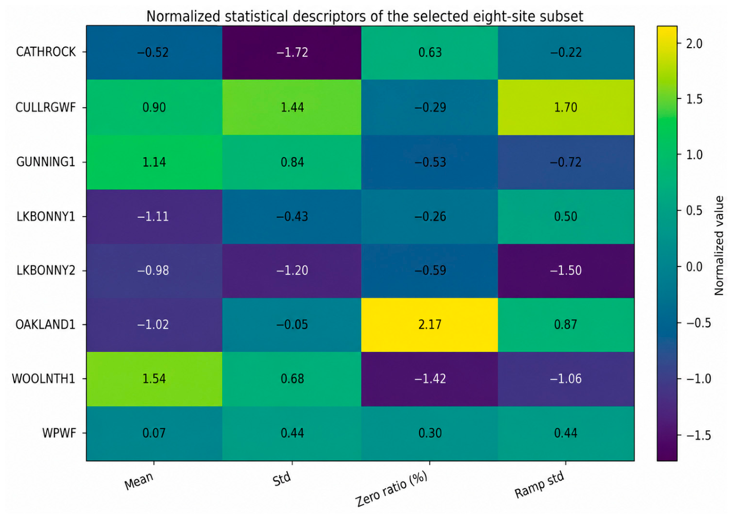
To further illustrate the diversity of the selected subset, Figure 1 presents the normalized site-level statistical descriptors. The figure clearly shows that the retained wind farms cover a broad range of operating levels, intermittency patterns, and ramping behaviors, thereby supporting the representativeness of the selected subset beyond the tabulated summary statistics.

Figure 1 summarizes the relative differences across sites in terms of mean production, production variability, zero-output ratio, and ramp variability, confirming that the retained subset preserves a broad range of operating regimes.

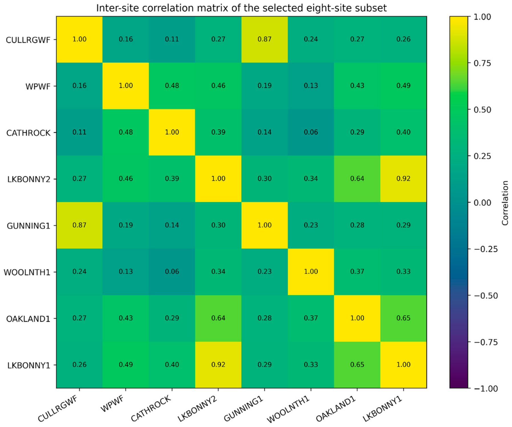
In addition, the statistical dependence between sites is visualized in Figure 2, which reports the inter-site correlation matrix of the selected subset. The presence of non-negligible cross-site dependencies supports the use of a graph-enhanced forecasting architecture and provides an empirical motivation for the prior graph construction adopted later in the proposed model.

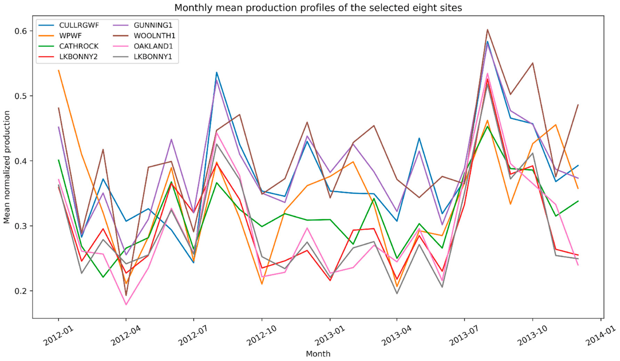
As an additional temporal illustration, Figure 3 shows the monthly mean production profiles of the selected wind farms over the study period. The figure highlights persistent differences in average generation level and temporal behavior across sites, further confirming that the selected subset captures diverse operating regimes rather than a narrow or homogeneous subset of the original benchmark.

Figure 3 illustrates the temporal diversity of the selected subset across the study period and highlights persistent differences in average generation levels among sites.

Overall, the combination of

Table 1. Statistical characteristics and functional role of the selected eight-site subset.

Site	Mean	Std	Zero Ratio	Ramp Std	Role in Subset
LKBONNY1	0.296	0.290	10.7%	0.0437	Low-output, irregular
OAKLAND1	0.300	0.298	20.7%	0.0450	Low-output, high intermittency
LKBONNY2	0.302	0.273	9.4%	0.0366	Intermediate, relatively stable
CATHROCK	0.321	0.262	14.3%	0.0411	Intermediate profile
WPWF	0.346	0.309	13.0%	0.0435	Medium-high variability
CULLRGWF	0.381	0.331	10.6%	0.0480	High variability
GUNNING1	0.390	0.318	9.6%	0.0394	High-output profile
WOOLNTH1	0.407	0.314	5.9%	0.0381	Highest-average output

and Figure 1, Figure 2 and Figure 3 confirms that the selected eight-site subset preserves the diversity of the original benchmark across production level, volatility, intermittency, temporal behavior, and inter-site dependence, while remaining compatible with repeated probabilistic training and comparative experiments. At the same time, the conclusions of the present study should be interpreted within the scope of this reduced benchmark setting.

3.3. Data Preparation and Feature Construction

3.3.1. Multi-Site Panel Construction

The raw data are first loaded from the Excel workbook and converted into a unified long-format table. For each site, timestamps are parsed, the target variable is cast to numeric format, and incomplete rows are removed. The site-level series are then merged into a shared panel indexed by time. To ensure temporal consistency across all sites, the panel is chronologically ordered and missing values are handled through time-based interpolation, followed by forward and backward filling when necessary.

3.3.2. Chronological Split and Site-Wise Standardization

To avoid temporal leakage, the dataset is divided chronologically into training, validation, and test subsets according to a 70%/15%/15% split. Standardization is then performed independently for each site using a StandardScaler fitted on the training segment only. The fitted transformation is subsequently applied to the full time series of the corresponding site. This design preserves local amplitude characteristics while ensuring that no future information contaminates the normalization process.

3.3.3. Static Site Descriptors

In addition to temporal variables, the model uses site-level static covariates computed from the training partition only. For each site, five descriptors are extracted: mean production, standard deviation of production, maximum production, standard deviation of the production ramp, and zero-production ratio. These variables are then standardized across sites and provided to the model as static real-valued covariates. Site identity is further encoded through a trainable embedding layer.

3.3.4. Historical Observed Variables

For each sample, past observed inputs are constructed from the standardized panel by a sliding-window procedure. Four variables are retained at each time step: scaled production, first-order ramp, rolling mean, and rolling standard deviation computed with a window of six time steps. Consequently, the historical input tensor has the form

$${\mathrm{X}}^{\left(\mathrm{p}\right)}\in {\mathrm{R}}^{\mathrm{N}\times \mathrm{T}\times \mathrm{S}\times {\mathrm{F}}_{\mathrm{p}}}$$

(1)

where N is the number of samples, T = 72 is the look-back length, S is the number of sites, and F_p = 4 denotes the number of past observed variables.

3.3.5. Future-Known Covariates and Forecasting Target

Future-known inputs are derived from deterministic calendar features, namely the sine and cosine encodings of hour-of-day, day-of-week, and month-of-year. These features are repeated across sites and organized as

$${\mathrm{X}}^{\left(\mathrm{f}\right)}\in {\mathrm{R}}^{\mathrm{N}\times \mathrm{H}\times \mathrm{S}\times {\mathrm{F}}_{\mathrm{f}}}$$

(2)

with H ∈ {1, 3, 6, 12} depending on the forecasting horizon considered in each experiment and F_f = 6. The forecasting target is the future scaled production tensor

$$Y\in R^{N\times H\times S}$$

(3)

This input design explicitly separates static covariates, past observed variables, and future-known variables in a way that is consistent with TFT-style forecasting.

3.4. Prior Spatial Graph Construction

To introduce structural dependence between sites, a prior adjacency matrix is estimated from the training data. The procedure relies on the absolute Pearson correlation matrix of the site-level production series. For each site, only the top-k most correlated neighbors are retained, with k = 5 in the present implementation. The resulting adjacency matrix is symmetrized, self-loops are added, and each row is normalized to sum to one. This yields a static prior graph that captures long-term inter-site similarity patterns.

This prior adjacency is not used as a fixed graph, but rather as a structural bias later combined with a sample-dependent dynamic graph inferred by the neural network itself.

3.5. Proposed DG-TFT-CQR Model

The proposed architecture, DG-TFT-CQR, builds on a TFT-style forecasting foundation by incorporating a dynamic graph block over encoder-side site representations. The conformal calibration stage is applied to the predicted quantiles after the fact during validation and test evaluation, rather than being built into the neural architecture.

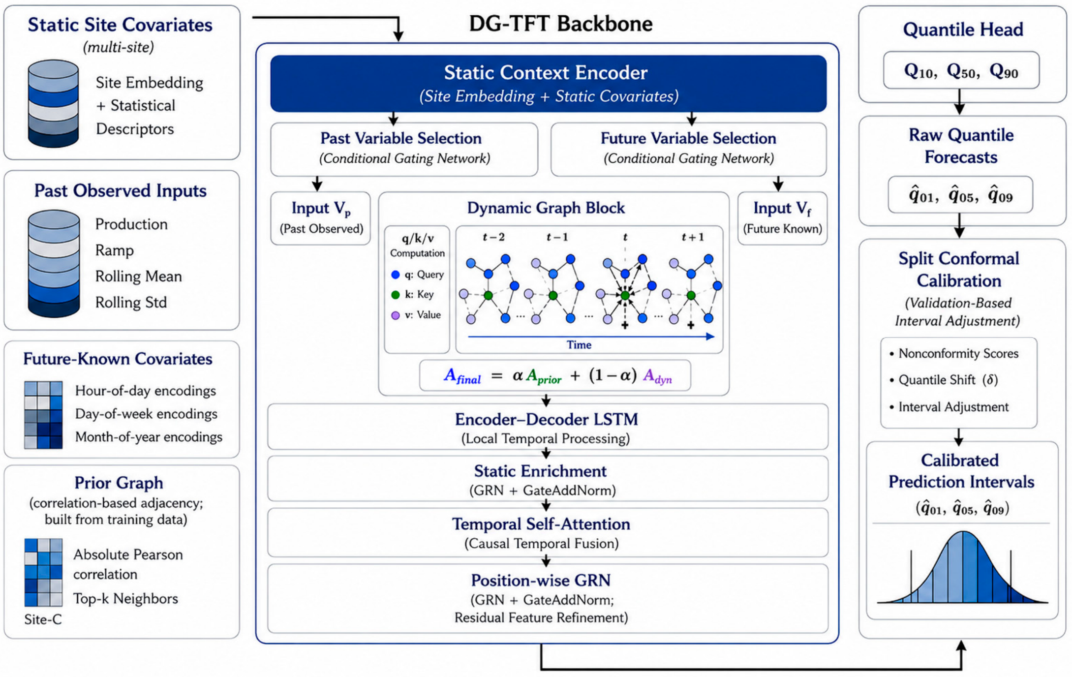
Figure 4 illustrates the overall structure of the proposed framework. The architecture is divided into three major components: input representations, the DG-TFT backbone, and probabilistic output with post hoc calibration. On the input side, four information sources are considered: static site covariates, previously observed inputs, future-known covariates, and a prior graph. Static site covariates combine learned site embeddings with standardized statistical descriptors, whereas the previous observed branch includes production-related temporal variables like production, ramp, rolling mean, and rolling standard deviation. The future branch includes known temporal encodings such as the hour of the day, day of the week, and month of the year. Finally, the prior graph summarizes correlation-based site relationships derived from the training data.

The framework in Figure 4 combines static site conditioning, conditional variable selection, encoder-side dynamic graph learning, encoder–decoder LSTM temporal modeling, static enrichment, causal temporal self-attention, position-wise gated refinement, quantile forecasting, and post hoc split conformal calibration for multi-site probabilistic wind power forecasting.

A static context encoder is the first component of the DG-TFT backbone to process static covariates. This module generates contextual representations that are used to condition downstream network components. In parallel, two distinct conditional variable selection networks process previously observed and future-known variables, allowing the model to adaptively weight the most informative inputs for the encoder and decoder branches. The dynamic graph block is a critical component of the proposed framework, as it operates on encoder-side representations derived from previous observations. At each time step, the model computes query, key, and value projections across sites, then creates a sparse dynamic adjacency matrix using top-k neighbor selection and combines it with the prior graph. The graph-enhanced past representation and the future-known representation are then processed through an encoder–decoder LSTM, followed by static enrichment, temporal self-attention with causal masking, and position-wise gated residual refinement. At the output stage, the refined decoder representations are projected through a quantile head to produce the raw predictive quantiles, which are then adjusted using split conformal calibration to obtain the final calibrated prediction intervals.

3.5.1. Static Encoding

Each site is represented by the concatenation of a learned embedding and the standardized static real-valued covariates. More formally, for each site sss, the static input is defined as

$${\mathrm{z}}_{\mathrm{s}}=\left[{\mathrm{e}}_{\mathrm{s}};{\mathrm{r}}_{\mathrm{s}}\right]$$

(4)

where e_s denotes the learned site embedding and r_s denotes the vector of standardized static real-valued descriptors. These inputs are processed by a static covariate encoder to produce a latent static representation

$${\mathrm{h}}_{\mathrm{s}}^{\mathrm{s}\mathrm{a}}={\mathrm{f}}_{\mathrm{s}\mathrm{t}\mathrm{a}\mathrm{t}}\left({\mathrm{z}}_{\mathrm{s}}\right)$$

(5)

together with four downstream context vectors used in subsequent components: a context for variable selection, a context for static enrichment, an initial hidden state for the LSTM, and an initial cell state for the LSTM, namely

$${\mathrm{h}}_{\mathrm{s}}^0={\mathrm{g}}_{\mathrm{h}}\left({\mathrm{h}}_{\mathrm{s}}^{\mathrm{s}\mathrm{a}}\right),{\mathrm{c}}_{\mathrm{s}}^0={\mathrm{g}}_{\mathrm{c}}\left({\mathrm{h}}_{\mathrm{s}}^{\mathrm{s}\mathrm{a}}\right)$$

(6)

3.5.2. Conditional Variable Selection

Past observed variables and future-known variables are processed separately by two Conditional Variable Selection Networks (VSNs). Each VSN receives both the temporal inputs and the static selection context, and outputs a weighted combination of variable-specific representations. Let ${\mathrm{X}}_{\mathrm{t},\mathrm{s}}\in {\mathrm{R}}^{\mathrm{F}}$ denote the input vector at time step t and site s, where F corresponds either to the number of past observed variables or to the number of future-known covariates. Each variable is first transformed through a dedicated context-conditioned nonlinear block

$${\mathrm{v}}_{\mathrm{t},\mathrm{s},\mathrm{j}}=\mathrm{G}\mathrm{R}{\mathrm{N}}_{\mathrm{j}}$$

(7)

Then, a context-conditioned weighting network produces normalized variable-selection weights

$${\mathsf{\pi }}_{\mathrm{t},\mathrm{s}}=\mathrm{s}\mathrm{o}\mathrm{f}\mathrm{t}\mathrm{m}\mathrm{a}\mathrm{x}\left(\mathrm{G}\mathrm{R}{\mathrm{N}}_{\mathrm{w}}\left({\mathrm{x}}_{\mathrm{t},\mathrm{s}},{\mathrm{c}}_{\mathrm{s}}^{\mathrm{s}\mathrm{l}}\right)\right)$$

(8)

The final selected representation is obtained as a weighted sum of the variable-specific hidden representations

$$\widetilde{{\mathrm{x}}_{\mathrm{t},\mathrm{s}}}={\displaystyle {\sum }_{\mathrm{j}=1}^{\mathrm{F}}}{\mathsf{\pi }}_{\mathrm{t},\mathrm{s},\mathrm{j}}{\mathrm{v}}_{\mathrm{t},\mathrm{s},\mathrm{j}}$$

(9)

This mechanism allows the model to adaptively emphasize the most informative variables as a function of site context and temporal configuration.

3.5.3. Dynamic Graph Block

A key extension of the model consists of a dynamic graph block applied to encoder-side temporal representations. At each historical time step, the model projects the site representations into query, key, and value spaces, computes pairwise similarity scores across sites, and constructs a sparse dynamic adjacency matrix by retaining only the top-k neighbors for each node.

Let ${\mathrm{X}}_{\mathrm{t}}^{\left(\mathrm{p}\right)}\in {\mathbb{R}}^{\mathrm{S}\mathrm{\ast }\mathrm{d}}$ denote the selected encoder-side representation across the S sites at historical step t, where d is the hidden representation size. Query, key, and value representations are obtained through three learnable linear transformations:

$${\mathrm{Q}}_{\mathrm{t}}=\widetilde{{\mathrm{X}}_{\mathrm{t}}^{\left(\mathrm{p}\right)}{\mathrm{W}}_{\mathrm{Q}}}$$

(10)

$${\mathrm{K}}_{\mathrm{t}}=\widetilde{{\mathrm{X}}_{\mathrm{t}}^{\left(\mathrm{p}\right)}{\mathrm{W}}_{\mathrm{K}}}$$

(11)

$${\mathrm{V}}_{\mathrm{t}}=\widetilde{{\mathrm{X}}_{\mathrm{t}}^{\left(\mathrm{p}\right)}{\mathrm{W}}_{\mathrm{V}}}$$

(12)

where ${\mathrm{W}}_{\mathrm{Q}};{\mathrm{W}}_{\mathrm{K}},{\mathrm{W}}_{\mathrm{v}}\in {\mathbb{R}}^{\mathrm{d}\mathrm{\ast }{\mathrm{d}}_{\mathrm{k}}}$ are trainable projection matrices and d_k denotes the projection dimension used for similarity computation.

The instantaneous similarity between all pairs of sites is computed using scaled dot-product attention

$${\mathrm{E}}_{\mathrm{t}}={\displaystyle \frac{{\mathrm{Q}}_{\mathrm{t}}{\mathrm{K}}_{\mathrm{t}}^{\mathrm{\top }}}{\sqrt{{\mathrm{d}}_{\mathrm{k}}}}}$$

(13)

where each element E_t(i,j) measures the dynamic affinity between site i and site j at time step t.

To reduce noise and avoid a fully connected graph, only the strongest k neighbors are retained for each site. The value k = 5 was selected as a compromise between graph sparsity and sufficient neighborhood information, preventing noisy fully connected interactions while preserving the strongest inter-site dependencies. A binary top-k mask M_t is constructed such that

$${\mathrm{M}}_{\mathrm{t}}(\mathrm{i},\mathrm{j})=\left\{\begin{array}{c}1, j\in \mathrm{TopK}\left({\mathrm{E}}_{\mathrm{t}}\right(i,:\left)\right)\\ 0, \mathrm{otherwise}\end{array}\right.$$

(14)

where $\mathrm{T}\mathrm{o}\mathrm{p}\mathrm{K}\left({\mathrm{E}}_{\mathrm{t}}\right(\mathrm{i},:\left)\right)$ denotes the set of the five largest similarity scores associated with site i.

$$\widetilde{{\mathrm{E}}_{\mathrm{t}}}={\mathrm{E}}_{\mathrm{t}}\odot {\mathrm{M}}_{\mathrm{t}}$$

(15)

where ⊙ denotes element-wise multiplication.

The sparse dynamic adjacency matrix is then obtained through row-wise softmax normalization

$${\mathrm{A}}_{\mathrm{t}}^{\mathrm{dyn}}\left(\mathrm{i},\mathrm{j}\right)={\displaystyle \frac{\exp \left(\widetilde{{\mathrm{E}}_{\mathrm{t}}}\left(\mathrm{i},\mathrm{j}\right)\right)}{{\sum }_{\mathrm{m}=1}^{\mathrm{S}}\exp \left(\widetilde{{\mathrm{E}}_{\mathrm{t}}}\left(\mathrm{i},\mathrm{m}\right)\right)}}$$

(16)

which guarantees that each row sums to one and therefore defines a valid graph aggregation operator.

The normalized dynamic graph is combined with the correlation-based prior graph introduced in Section 3.4

$${\mathrm{A}}_{\mathrm{t}}^{\mathrm{blend}}=\mathsf{\alpha }{\mathrm{A}}^{\mathrm{prior}}+\left(1-\mathsf{\alpha }\right){\mathrm{A}}_{\mathrm{t}}^{\mathrm{dyn}}$$

(17)

where ${\mathrm{A}}^{\mathrm{prior}}$ denotes the correlation-based adjacency matrix described in Section 3.4 and α = 0.30 controls the contribution of the prior graph relative to the dynamically inferred graph.

Where ${\mathrm{A}}^{\mathrm{prior}}$ denotes the prior adjacency matrix and α = 0.30 controls the trade-off between long-term structural dependencies and short-term dynamic interactions.

The blended matrix ${\mathrm{A}}_{\mathrm{t}}^{\mathrm{blend}}$ combines structural information from the prior graph and sample-dependent information extracted from the current input sequence.

A second row-normalization step is applied after blending in order to preserve stochasticity of the final adjacency matrix

$${\mathrm{A}}_{\mathrm{t}}={\mathrm{D}}_{\mathrm{t}}^{-1}{\mathrm{A}}_{\mathrm{t}}^{\mathrm{blend}}$$

(18)

where D_t is the diagonal degree matrix associated with $A_t^{\mathrm{blend}}$

$${\mathrm{D}}_{\mathrm{t}}\left(\mathrm{i},\mathrm{i}\right)={\sum }_{\mathrm{j}=1}^{\mathrm{S}}{\mathrm{A}}_{\mathrm{t}}^{\mathrm{blend}}\left(\mathrm{i},\mathrm{j}\right)$$

(19)

The resulting matrix ${\mathrm{W}}_{\mathrm{v}}\in {\mathbb{R}}^{\mathrm{S}\mathrm{\ast }\mathrm{S}}$ is used for graph propagation and neighborhood aggregation.

The graph-aggregated representation is computed as

$${\mathrm{G}}_{\mathrm{t}}={\mathrm{A}}_{\mathrm{t}}{\mathrm{V}}_{\mathrm{t}}$$

(20)

where each site representation becomes a weighted aggregation of information received from its dynamically selected neighboring sites.

And the resulting graph-enhanced representation is passed through a gated residual normalization block

$$\widehat{{\mathrm{H}}_{\mathrm{t}}}=\mathrm{LayerNorm}\left({\mathrm{H}}_{\mathrm{t}}+{\mathrm{G}}_{\mathrm{t}}\right)$$

(21)

This residual fusion mechanism preserves the original temporal representation while incorporating dynamically learned spatial interactions. The graph-enhanced representation $\widehat{{\mathrm{H}}_t}$ is subsequently forwarded to the encoder–decoder LSTM module described in Section 3.5.4.

3.5.4. Local Temporal Processing

The graph-enhanced encoder inputs and the decoder future-known representations are reshaped site-wise and processed by an encoder–decoder LSTM with hidden size 64 and one recurrent layer. The encoder states are initialized using the static context vectors described above. Formally, for each site s, the encoder processes the graph-enhanced historical sequence as

$${\mathrm{H}}_{1:\mathrm{T},\mathrm{s}}^{\mathrm{e}\mathrm{n}\mathrm{c}}={\mathrm{L}\mathrm{S}\mathrm{T}\mathrm{M}}_{\mathrm{e}\mathrm{n}\mathrm{c}}\widehat{{(\mathrm{H}}_{1:\mathrm{T},\mathrm{s}})}$$

(22)

While the decoder processes the selected future-known sequence using the final encoder state

$${\mathrm{H}}_{1:\mathrm{T},\mathrm{s}}^{\mathrm{d}\mathrm{e}\mathrm{c}}={\mathrm{L}\mathrm{S}\mathrm{T}\mathrm{M}}_{\mathrm{d}\mathrm{e}\mathrm{c}}\left(\widetilde{{\mathrm{x}}_{1:\mathrm{T},\mathrm{s}}}\right)$$

(23)

After the local temporal modeling stage, a gated residual connection is applied to preserve lower-level information and stabilize optimization. The concatenated encoder–decoder representation is therefore written as

$${\mathrm{H}}_{1:\mathrm{T}+\mathrm{H},\mathrm{s}}^{\mathrm{f}\mathrm{s}}=\mathrm{G}\mathrm{a}\mathrm{t}\mathrm{e}\mathrm{A}\mathrm{d}\mathrm{d}\mathrm{N}\mathrm{o}\mathrm{r}\mathrm{m}\left(\right[{\mathrm{H}}_{1:\mathrm{T},\mathrm{s}}^{\mathrm{e}\mathrm{n}\mathrm{c}};{\mathrm{H}}_{1:\mathrm{T},\mathrm{s}}^{\mathrm{d}\mathrm{e}\mathrm{c}}\left]\right)$$

(24)

3.5.5. Static Enrichment and Temporal Attention

The concatenated encoder–decoder sequence is enriched using the static context through a dedicated static enrichment Gated Residual Network. This step can be written as

$${\mathrm{H}}_{1:\mathrm{T}+\mathrm{H},\mathrm{s}}^{\mathrm{S}\mathrm{E}}=\mathrm{G}\mathrm{R}{\mathrm{N}}_{\mathrm{e}\mathrm{n}\mathrm{r}}\left({\mathrm{H}}_{1:\mathrm{T}+\mathrm{H},\mathrm{s}}^{\mathrm{f}\mathrm{s}}\right)$$

(25)

Subsequently, an interpretable temporal self-attention layer with four heads is applied over the full sequence. A causal mask ensures that no temporal position attends to information located ahead in time. The attention block is therefore expressed as

$${\mathrm{H}}^{\mathrm{A}\mathrm{T}\mathrm{T}}=\mathrm{MultiHead}!\left({\mathrm{H}}^{\mathrm{S}\mathrm{E}},{\mathrm{H}}^{\mathrm{S}\mathrm{E}},{\mathrm{H}}^{\mathrm{S}\mathrm{E}},{\mathrm{M}}_{\mathrm{c}\mathrm{a}\mathrm{u}\mathrm{s}\mathrm{a}\mathrm{l}}\right)$$

(26)

This attention mechanism allows the model to capture long-range temporal dependencies beyond the local receptive field of the LSTM. The attended sequence is further refined through a position-wise gated residual feed-forward block before the decoder-side outputs are extracted for final prediction. This refinement step is written as

$${\mathrm{H}}_{1:\mathrm{T}+\mathrm{H},\mathrm{s}}^{\mathrm{f}\mathrm{s}}=\mathrm{G}\mathrm{a}\mathrm{t}\mathrm{e}\mathrm{A}\mathrm{d}\mathrm{d}\mathrm{N}\mathrm{o}\mathrm{r}\mathrm{m}$$

Finally, only the decoder-side outputs are retained for prediction

$${\mathrm{H}}_{1:\mathrm{H},\mathrm{s}}^{\mathrm{o}\mathrm{u}\mathrm{t}}={\mathrm{H}}_{1:\mathrm{T}+\mathrm{H},\mathrm{s}}^{\mathrm{f}\mathrm{s}}$$

(27)

3.5.6. Quantile Output Layer

The decoder representations are finally projected to three quantiles, ${\mathrm{q}}_{0.1}$, ${\mathrm{q}}_{0.5}$, and ${\mathrm{q}}_{0.9}$, for each site and forecast step.

This step can be written as

$$\widehat{{\mathrm{Q}}_{1:\mathrm{H},\mathrm{s}}^{\mathrm{r}\mathrm{a}\mathrm{w}}}={{\mathrm{W}}_{\mathrm{Q}}\mathrm{H}}_{1:\mathrm{H},\mathrm{s}}^{\mathrm{o}\mathrm{u}\mathrm{t}}$$

(28)

To guarantee quantile monotonicity, the outputs are explicitly sorted along the quantile dimension:

$$\widehat{{\mathrm{Q}}_{1:\mathrm{H},\mathrm{s}}}=\mathrm{s}\mathrm{o}\mathrm{r}\mathrm{t}\left(\widehat{{\mathrm{Q}}_{1:\mathrm{H},\mathrm{s}}^{\mathrm{r}\mathrm{a}\mathrm{w}}}\right)$$

(29)

ensuring $q_{0.1}\le q_{0.5}\le q_{0.9}$ for all samples and sites. That is,

$$\widehat{{\mathrm{q}}_{0.1}}\le \widehat{{\mathrm{q}}_{0.5}}\le \widehat{{\mathrm{q}}_{0.9}}$$

(30)

Although explicit sorting effectively prevents quantile crossing and guarantees monotonic prediction intervals, it is used as a post-processing operation and thus has no direct influence on the learning dynamics of quantile outputs. Other approaches reported in the literature include monotonic quantile parameterization, which predicts higher quantiles with positive cumulative increments, and quantile-crossing penalty terms added to the training objective. These approaches require monotonicity during optimization rather than after prediction. Explicit sorting was chosen for this project because of its simplicity, numerical stability, and low computational overhead.

3.6. Algorithm for the Proposed DG-TFT-CQR Framework

To synthesize the full methodological workflow, Algorithm 1 summarizes the complete DG-TFT-CQR pipeline from data preparation to calibrated probabilistic forecasting. The procedure follows the actual implementation used in the experiments and highlights the interaction between multi-site feature construction, prior graph estimation, dynamic graph learning, TFT-based temporal fusion, quantile forecasting, and post hoc conformal calibration.

Algorithm 1. Training and inference procedure of DG-TFT-CQR

Input: Multi-sheet Excel workbook containing synchronized site-level wind power series; look-back length T; forecasting horizon H; quantile set Q = {0.1, 0.5, 0.9}; top-k neighborhood size; graph blending coefficient α. Output: Median forecasts, calibrated prediction intervals, global metrics, site-wise metrics, and horizon-wise metrics. 1. Load the multi-site Excel workbook and construct a unified temporal panel indexed by timestamp and site. 2. Sort the panel chronologically and impute missing values using time interpolation followed by forward/backward filling. 3. Split the panel chronologically into training, validation, and test subsets. 4. Fit one scaler per site on the training subset only, then standardize the full panel using these site-specific transformations. 5. Compute static site descriptors from the training subset only, including mean production, production standard deviation, maximum production, ramp standard deviation, and zero-production ratio. 6. Construct deterministic future-known calendar covariates using sine/cosine encodings of hour-of-day, day-of-week, and month-of-year. 7. Generate supervised samples by a sliding-window procedure. 8. Estimate the prior spatial adjacency matrix from the absolute Pearson correlation matrix of the training panel and retain the top-k neighbors per site. 9. Initialize DG-TFT-CQR with site embeddings, static covariate encoder, conditional variable selection networks, dynamic graph block, encoder–decoder LSTM backbone, static enrichment layer, interpretable temporal attention, position-wise gated residual network, and quantile output head. 10. In each training epoch, use forward propagation, quantile loss minimization, gradient clipping, and Adam updates. 11. Monitor validation loss and retain the best model based on early stopping. 12. Apply inference to the validation and test sets to obtain raw quantile forecasts. 13. For each site, inverse-transform forecasts and targets to their original scale. 14. Calculate the conformal nonconformity scores for the validation set and estimate the pooled calibration threshold. 15. Using the conformal threshold, expand the test set’s lower and upper raw quantiles to obtain calibrated prediction intervals. 16. Assess point forecasts using MAE, RMSE, and R2, and probabilistic forecasts using pinball loss, PICP, PINAW, and interval score. 17. Export global metrics, site metrics, horizon metrics, and calibrated predictions.

3.7. Hyperparameter Settings

The DG-TFT-CQR hyperparameters, summarized in

Table 2. Hyperparameter configuration of DG-TFT-CQR.

Category	Hyperparameter	Value
Data window	Look-back length T	72
Forecasting setup	Horizon H	{1, 3, 6, 12} depending on the experiment
Data split	Train/Val/Test	70%/15%/15%
Optimization	Optimizer	Adam
Optimization	Learning rate	1 × ${10}^{-3}$
Optimization	Weight decay	1 × ${10}^{-5}$
Optimization	Batch size	300
Optimization	Maximum epochs	200
Optimization	Early stopping patience	20
Optimization	Gradient clipping	1.0
Reproducibility	Random seed	42
Static encoding	Site embedding dimension	16
Static encoding	Static hidden dimension	32
Backbone	Hidden size	64
Backbone	LSTM layers	1
Backbone	Dropout	0.15
Temporal attention	Number of heads	4
Dynamic graph	Top-k neighbors	5
Dynamic graph	Graph blending coefficient α	0.30
Probabilistic output	Quantiles	{0.1, 0.5, 0.9}
Conformal calibration	Miscoverage level α	0.10

, were chosen for multi-site wind power forecasting to strike a balance between computational efficiency, training stability, and predictive accuracy. The look-back window was set to T = 72, which corresponds to six hours of historical data with a five-minute temporal resolution. In contrast, the forecasting horizon was varied in four different experiments (H = 1, H = 3, H = 6, and H = 12), with forecast lead times of 5, 15, 30, and 60 min, respectively. The dataset was divided chronologically into training, validation, and test subsets using a 70%/15%/15% ratio. The model was optimized using the Adam optimizer, with a learning rate of 10⁻³ and a weight decay of 10⁻⁵. The batch size was set to 300, the maximum number of training epochs to 200, and early stopping was used after 20 epochs based on the validation pinball loss. Gradient clipping with a maximum norm of 1.0 was used to improve optimization stability. All experiments were conducted with a random seed of 42 to ensure reproducibility.

On the architectural side, the site embedding dimension was fixed to 16, the static hidden dimension to 32, and the main latent representation size to 64. The encoder and decoder recurrent blocks each used one LSTM layer, the dropout rate was set to 0.15, and the interpretable temporal attention module employed four attention heads. In the dynamic graph component, the number of retained neighbors was fixed to k = 5, and the final graph adjacency matrix was obtained by combining the prior graph and the dynamic graph with a convex blending coefficient α = 0.30. Probabilistic forecasting was performed through three output quantiles, namely $q_{0.1}$, $q_{0.5}$ and $q_{0.9}$. Finally, split conformal calibration was applied with α = 0.10, corresponding to a nominal 90% prediction interval.

3.8. Training Objective and Optimization Strategy

All experiments were conducted in Google Colab (Google LLC, Mountain View, CA, USA) using Python (version 3.12.13; Python Software Foundation, Wilmington, DE, USA) and the PyTorch deep learning framework (version 2.11.0 with CUDA 12.8; PyTorch Foundation, San Francisco, CA, USA). The model was trained using the Adam optimizer. The training objective is the standard quantile loss (pinball loss):

$${\mathcal{L}}_{\mathcal{q}}\left(\mathrm{y},\widehat{{\mathrm{y}}^{\left(\mathrm{q}\right)}}\right)=\max \left(\mathrm{q}\left(\mathrm{y}-\widehat{{\mathrm{y}}^{\left(\mathrm{q}\right)}}\right),\left(\mathrm{q}-1\right)\left(\mathrm{y}-\widehat{{\mathrm{y}}^{\left(\mathrm{q}\right)}}\right)\right)$$

(31)

where y denotes the observed target value, $\widehat{{\mathrm{y}}^{\left(\mathrm{q}\right)}}$) denotes the predicted quantile associated with quantile level q, and q ∈ (0,1). The pinball loss penalizes overestimation and underestimation asymmetrically according to the selected quantile level. During training, the total objective is obtained by averaging the loss over all samples, sites, forecasting horizons, and predicted quantiles {0.1, 0.5, 0.9}.

During training, the validation pinball loss is monitored, and the best model is retained according to early stopping. Gradient clipping with a maximum norm of 1.0 is applied to improve optimization stability.

3.9. Conformal Calibration

To improve the empirical reliability of the predicted intervals, the raw quantile outputs are post-processed through split conformal calibration on the validation set.

It should be noted that the neural network first predicts three raw quantiles, namely $\widehat{{\mathrm{q}}_{0.1}}$, $\widehat{{\mathrm{q}}_{0.5}}$, and $\widehat{{\mathrm{q}}_{0.9}}$. Before calibration, the interval between $\widehat{{\mathrm{q}}_{0.1}}$ and $\widehat{{\mathrm{q}}_{0.9}}$ corresponds to a central 80% predictive interval. The nominal 90% interval reported in this study is obtained after the split conformal calibration step.

Let $\widehat{{\mathrm{q}}_{0.1}}$ and $\widehat{{\mathrm{q}}_{0.9}}$ denote the lower and upper predicted quantiles, respectively. For each validation observation y, the nonconformity score is defined as

$$\mathrm{s}=\mathrm{m}\mathrm{a}\mathrm{x}\{\widehat{{\mathrm{q}}_{0.1}}-\mathrm{y},\mathrm{y}-\widehat{{\mathrm{q}}_{0.9}},0\}$$

(32)

where s measures the amount by which the observed value falls outside the raw 80% predictive interval.

A pooled quantile threshold $\widehat{{\mathrm{q}}_{\mathsf{\alpha }}}$ is then estimated across all validation samples for α = 0.10, corresponding to a target marginal coverage level of 90%. The calibrated interval is obtained as

$$\widetilde{{\mathrm{q}}_{0.1}}=\widehat{{\mathrm{q}}_{0.1}}-\widehat{{\mathrm{q}}_{\mathsf{\alpha }}},\widetilde{{\mathrm{q}}_{0.9}}=\widehat{{\mathrm{q}}_{0.9}}+\widehat{{\mathrm{q}}_{\mathsf{\alpha }}}$$

(33)

Thus, the raw interval between $\widehat{{\mathrm{q}}_{0.1}}$ and $\widehat{{\mathrm{q}}_{0.9}},$ should be interpreted as an 80% quantile interval, whereas the final interval between q-tilde 0.1 and q-tilde 0.9 is the conformally calibrated interval designed to achieve approximately 90% marginal coverage.

This calibration step adjusts interval width in a distribution-free manner while leaving the point forecast unchanged. In practical terms, the conformal layer acts as a post hoc reliability correction applied after model training and raw quantile inference.

In the present study, a pooled split conformal strategy is adopted to provide a simple, stable, and uniform calibration layer across sites and forecast steps. This choice is motivated by operational simplicity and by the desire to apply the same post-processing rule across all forecasting settings considered in the benchmark. However, this design also implies that the calibration layer may smooth out part of the site-specific and horizon-specific heterogeneity in predictive uncertainty.

For this reason, the conformal stage should not be interpreted as a universally optimal calibration design for multi-site wind forecasting. Rather, it is used here as a practical reliability-oriented post-processing mechanism that can be consistently integrated into the DG-TFT-CQR pipeline. Its main role is to improve empirical coverage and probabilistic interpretability, not to guarantee superiority on every individual interval-based metric.

More specialized calibration strategies, such as horizon-conditional, site-conditional, or locally adaptive conformal procedures, may further improve the calibration–sharpness trade-off. These extensions are beyond the scope of the present study but represent an important direction for future research in uncertainty-aware multi-site renewable energy forecasting.

3.10. Evaluation Protocol

Model performance is evaluated both globally and by site. Following an inverse transformation to the original scale, the standard point-forecast metrics MAE, RMSE, and R are computed using the median forecast q0.5.

For training purposes, the wind power series are normalized. However, all reported deterministic performance metrics are derived from inverse transformation and expressed in the original power unit (kW). As a result, the reported MAE and RMSE values reflect actual forecasting errors in physical power units and can be interpreted directly from an operational perspective.

Raw quantile forecasts are evaluated using pinball loss, while calibrated prediction intervals are evaluated using the Prediction Interval Coverage Probability (PICP), Prediction Interval Normalized Average Width (PINAW), and Interval Score at 90% confidence level. In addition, the experimental pipeline offers metrics by site, global aggregated metrics, and forecasting horizon. The final results are exported as Excel files containing global results, site-specific metrics, horizon-specific metrics, and calibrated and uncalibrated predictions for each site and timestamp.

To ensure a fair comparison, all benchmark models are evaluated using the same train/validation/test sequence, preprocessing pipeline, forecasting horizon definitions, and overall evaluation protocol. This includes consistent data scaling, identical horizon settings, and shared evaluation metrics among all competing approaches. Although each model family could potentially benefit from architecture-specific hyperparameter tuning, the current benchmark prioritizes protocol consistency across models over exhaustive model-by-model optimization.

Furthermore, following consistency verification, all benchmark, ablation, and probabilistic result tables presented in the manuscript are meant to be produced from the same completed experimental pipeline. Ensuring comparability across models, horizons, and probabilistic settings is the goal of this design. As a result, a controlled comparative study using a single experimental protocol should be used to interpret the reported results.

In addition to global average performance, the manuscript examines deployment relevance through complexity analysis, inferential support through statistical significance testing, spatial robustness through site-wise evaluation, and component importance through ablation analysis. This more comprehensive protocol seeks to evaluate whether the suggested model offers more dependable and operationally significant forecasting behavior across various sites and time horizons, in addition to whether it lowers pointwise error.

3.11. Summary of the Methodological Contribution

In conclusion, the contribution of DG-TFT-CQR should be viewed as an architectural integration strategy rather than the introduction of new standalone forecasting modules. The framework incorporates (i) global multi-site supervised learning, (ii) site-aware static conditioning, (iii) conditional variable selection, (iv) encoder-side dynamic graph refinement, (v) TFT-style local and long-range temporal fusion, (vi) direct multi-quantile forecasting, and (vii) conformalized prediction interval calibration into a single forecasting pipeline. This formulation is ideal for operational wind power forecasting because it combines temporal dependence, evolving spatial inter-site interactions, predictive uncertainty, and interval reliability into a unified framework. As a result, the current study’s primary methodological contribution is the coordinated integration of these complementary capabilities, rather than the creation of fundamentally new graph-learning, Transformer, quantile-regression, or conformal-prediction modules.

4. Results

This section provides an empirical assessment of the proposed DG-TFT-CQR model from six complementary perspectives. First, the global point-forecasting accuracy is calculated for four prediction horizons: H1, H3, H6, and H12. Second, interval-based metrics are used to evaluate the accuracy of probabilistic predictions. Third, a site-specific analysis is carried out to determine the model’s spatial robustness across all eight wind farms. Fourth, ablation studies are used to assess the relative importance of the major architectural components. Fifth, formal statistical tests are run to see if the observed performance differences are statistically valid. Finally, a complexity analysis is used to evaluate the proposed architecture’s accuracy-efficiency trade-off. Furthermore, a small set of representative daily forecasting examples is provided to demonstrate the model’s behavior under favorable, typical, and challenging forecasting conditions.

Benchmark, ablation, statistical, and complexity analyses were conducted in four experimental settings, representing forecasting horizons H ∈ {1, 3, 6, 12}.

For clarity, lower values indicate better performance for MAE, RMSE, pinball loss, PINAW, and interval score, whereas higher values indicate better performance for R2. For PICP, the best result is the one closest to the nominal target coverage.

4.1. Benchmark Comparison of Point Forecasting Performance

Table 3. Consolidated benchmark results for point forecasting across H1, H3, H6, and H12.

Horizon	Model	MAE (kW)	RMSE (kW)	R2
H1	DG-TFT-CQR	0.025490	0.043186	0.980096
	Graph WaveNet	0.026171	0.043351	0.979943
	TSG-Net	0.025940	0.043573	0.979738
	CNN-LSTM-CQR	0.025841	0.043594	0.979718
	Quantile_LSTM	0.025872	0.043595	0.979717
	CNN-LSTM	0.026189	0.043628	0.978589
	MTGNN	0.026237	0.043746	0.979576
	LSTM	0.026143	0.043759	0.979565
	TCN	0.026129	0.043780	0.979545
	STGCN	0.026445	0.043870	0.979460
	Transformer	0.026319	0.044198	0.979152
	PatchTST	0.026634	0.044272	0.979082
	NLinear	0.026820	0.044937	0.978449
	DLinear	0.027278	0.045031	0.978359
	Quantile_Transformer	0.028169	0.045647	0.977763
	TimesNet	0.030351	0.047563	0.975856
	MDN_Meta_Reptile	0.240318	0.282127	0.150538
H3	DG-TFT-CQR	0.037241	0.062569	0.958221
	Graph WaveNet	0.046143	0.074520	0.940735
	MTGNN	0.045855	0.074632	0.940556
	STGCN	0.046578	0.075232	0.939596
	CNN-LSTM	0.046529	0.075291	0.936251
	TSG-Net	0.047009	0.075530	0.939117
	CNN-LSTM-CQR	0.045811	0.075709	0.938828
	Transformer	0.046581	0.075744	0.938772
	LSTM	0.046463	0.075816	0.938655
	Quantile_LSTM	0.046004	0.075883	0.938547
	TCN	0.046938	0.075929	0.938472
	PatchTST	0.047339	0.076097	0.938199
	Quantile_Transformer	0.046193	0.076299	0.937871
	TimesNet	0.050163	0.077945	0.935162
	DLinear	0.048371	0.077978	0.935107
	NLinear	0.048769	0.078439	0.934338
	MDN_Meta_Reptile	0.240696	0.282460	0.148530
H6	DG-TFT-CQR	0.047917	0.079747	0.932133
	Graph WaveNet	0.064469	0.099484	0.894376
	MTGNN	0.064083	0.099775	0.893758
	STGCN	0.064817	0.100667	0.891849
	CNN-LSTM	0.064933	0.100517	0.886691
	TSG-Net	0.064892	0.100720	0.891736
	Transformer	0.064899	0.100774	0.891619
	LSTM	0.064724	0.101302	0.890481
	PatchTST	0.065237	0.101240	0.890615
	TCN	0.065218	0.101609	0.889816
	Quantile_LSTM	0.063822	0.101629	0.889772
	CNN-LSTM-CQR	0.063550	0.101641	0.889747
	Quantile_Transformer	0.064164	0.101976	0.889019
	DLinear	0.066869	0.103645	0.885355
	TimesNet	0.068586	0.103867	0.884864
	NLinear	0.066728	0.104309	0.877984
	MDN_Meta_Reptile	0.241135	0.283149	0.144371
H12	DG-TFT-CQR	0.062891	0.102751	0.887340
	MTGNN	0.088503	0.130549	0.818114
	Graph WaveNet	0.088449	0.130876	0.817201
	STGCN	0.088959	0.132090	0.813795
	TSG-Net	0.090857	0.132269	0.813288
	CNN-LSTM	0.089721	0.132501	0.803792
	Transformer	0.090877	0.132852	0.811639
	PatchTST	0.089975	0.133438	0.809974
	TCN	0.091354	0.133647	0.809378
	LSTM	0.090387	0.133896	0.808668
	Quantile_Transformer	0.088045	0.134609	0.806625
	Quantile_LSTM	0.088090	0.134759	0.806194
	CNN-LSTM-CQR	0.087915	0.135500	0.804056
	DLinear	0.091852	0.136065	0.802418
	TimesNet	0.095381	0.136193	0.802045
	NLinear	0.091306	0.138770	0.794485
	MDN_Meta_Reptile	0.242502	0.284563	0.135807

Note: Because the evaluation metrics are reported in the original power scale (kW), the obtained MAE and RMSE values correspond to actual forecasting errors rather than normalized quantities. This simplifies the operational interpretation of forecasting performance across horizons.

presents the consolidated benchmark comparison of DG-TFT-CQR against the main competing baselines across the four forecasting horizons. The evaluation is based on MAE, RMSE, and R2, thereby providing a comprehensive view of both absolute- and squared-error behavior.

The benchmark comparison includes a diverse set of competing models from both traditional forecasting literature and recent time-series and spatio-temporal forecasting studies. The evaluated baselines include CNN-LSTM-CQR, Quantile-LSTM, TSG-Net, TCN, LSTM, CNN-LSTM, Transformer, Quantile-Transformer, MDN-Meta-Reptile, PatchTST, TimesNet, DLinear, NLinear, MTGNN, Graph WaveNet, and STGCN. This selection offers a comprehensive benchmark that includes recurrent, convolutional, Transformer-based, quantile-based, linear, and graph-based forecasting architectures.

DG-TFT-CQR had the best point-forecasting performance across all horizons, as Table 3 illustrates. As might be expected in a very short-term setting where local persistence is already highly informative, the performance gap over the strongest competitors remained relatively small at H1. Even in the most advantageous forecasting regime for simpler baselines, the suggested model continued to rank first simultaneously in MAE, RMSE, and R2, suggesting that the gain is already apparent.

The benchmark strengthens the proposed model by incorporating recent cutting-edge forecasting architectures from both the time-series and spatio-temporal forecasting literature, namely PatchTST, TimesNet, DLinear, NLinear, MTGNN, Graph WaveNet, and STGCN. This broader comparison confirms that DG-TFT-CQR is still competitive not only against traditional recurrent and Transformer-based baselines, but also with modern graph neural network and foundation-style forecasting models.

At H1, forecasting is relatively simple because the wind power series already exhibits strong short-term temporal persistence. As a result, the performance differences between the leading models are still relatively small. Nonetheless, DG-TFT-CQR has the best overall results with an RMSE of 0.043186, outperforming the strongest competing baseline, Graph WaveNet (RMSE = 0.043351).

The superiority of DG-TFT-CQR becomes increasingly evident as the forecasting horizon increases. With an RMSE of 0.074520 at H3, Graph WaveNet is the strongest competitor, whereas DG-TFT-CQR lowers the error to 0.062569, a 16.04% improvement. In comparison to Graph WaveNet, the RMSE improvement at H6 is roughly 19.84% (0.099484 versus 0.079747). At H12, DG-TFT-CQR achieves 0.102751, a 21.29% improvement, while MTGNN becomes the strongest competing baseline with an RMSE of 0.130549.

The fact that the top-performing rival models are mostly graph-based architectures like Graph WaveNet, MTGNN, and STGCN is a significant discovery. These models consistently outperform purely temporal methods such as PatchTST, TimesNet, DLinear, and NLinear over all forecasting horizons. This result highlights the necessity of explicitly modeling inter-site interactions and spatial dependencies in multi-site wind power forecasting problems.

The benchmark results generally support the conclusion that the proposed architecture is competitive at short horizons and becomes more advantageous as temporal uncertainty increases.

4.2. Probabilistic Forecasting Performance

Table 4. Consolidated probabilistic forecasting results across H1, H3, H6, and H12. For PICP, the best value is the one closest to the nominal 90% level.

Horizon	Model	Pinball	PICP	PINAW	Interval Score
H1	DG-TFT-CQR	0.008289	0.887562	0.094770	0.156348
	CNN-LSTM-CQR	0.008418	0.890326	0.096990	0.159734
	Quantile_LSTM	0.008650	0.883757	0.099794	0.166258
	Quantile_Transformer	0.009233	0.876774	0.102044	0.176266
	MDN_Meta_Reptile	—	0.786705	0.690362	1.170688
H3	DG-TFT-CQR	0.012120	0.889894	0.138525	0.229642
	CNN-LSTM-CQR	0.014966	0.892408	0.174544	0.283573
	Quantile_LSTM	0.015236	0.887721	0.175802	0.294251
	Quantile_Transformer	0.015364	0.891371	0.180071	0.298672
	MDN_Meta_Reptile	—	0.784788	0.689958	1.173919
H6	DG-TFT-CQR	0.015623	0.891503	0.179016	0.294191
	CNN-LSTM-CQR	0.020722	0.890733	0.240426	0.392851
	Quantile_LSTM	0.020985	0.884015	0.242053	0.398799
	Quantile_Transformer	0.021169	0.889902	0.247991	0.407404
	MDN_Meta_Reptile	—	0.950339	0.967935	1.937042
H12	DG-TFT-CQR	0.020478	0.891706	0.236781	0.386924
	CNN-LSTM-CQR	0.028586	0.891961	0.337239	0.537562
	Quantile_Transformer	0.028807	0.885963	0.336191	0.542019
	Quantile_LSTM	0.028821	0.895472	0.349935	0.542030
	MDN_Meta_Reptile	—	0.782544	0.691412	1.188797

summarizes the probabilistic forecasting performance of the proposed model and the main uncertainty-aware baselines using pinball loss, PICP, PINAW and interval score.

The probabilistic results confirm that DG-TFT-CQR provides the best overall trade-off between predictive sharpness, coverage reliability, and interval quality across the four forecasting horizons. Across all horizons, the proposed model achieved the lowest pinball loss, the narrowest prediction intervals, and the best interval score, while maintaining empirical coverage consistently close to the nominal 90% target. Although DG-TFT-CQR does not systematically achieve the PICP value closest to 0.90 at every horizon, it remains the most balanced probabilistic model overall. This pattern is particularly clear at H3, H6, and H12, where the gains in pinball loss, PINAW, and interval score over the competing baselines become substantial. Therefore, Table 4 supports the conclusion that DG-TFT-CQR is the strongest overall probabilistic model in the benchmark, although not necessarily the best on every individual metric taken in isolation.

4.3. Site-Wise RMSE Analysis

To determine whether the superiority of DG-TFT-CQR is also preserved locally, a site-wise RMSE analysis was conducted across the eight wind farms of the AEMO dataset.

Table 5. Average site-wise RMSE (kW) across the benchmark models. Lower values indicate better local forecasting accuracy.

Site	DG-TFT-CQR	CNN-LSTM-CQR	TSG-Net	CNN-LSTM	TCN	LSTM	MDN_Meta_Reptile	Quantile_LSTM	Quantile_Transformer
CATHROCK	0.066218	0.081393	0.082046	0.080806	0.082444	0.081025	0.282325	0.081248	0.081689
CULLRGWF	0.080772	0.099286	0.096788	0.099607	0.098785	0.099251	0.287676	0.099279	0.100153
GUNNING1	0.071639	0.089951	0.087854	0.089678	0.089407	0.089761	0.281047	0.089719	0.090586
LKBONNY1	0.072224	0.088391	0.087347	0.087729	0.088983	0.088243	0.281396	0.088477	0.089465
LKBONNY2	0.064523	0.080592	0.079618	0.079930	0.080793	0.080655	0.277969	0.080624	0.081485
OAKLAND1	0.076901	0.094974	0.093271	0.093913	0.095091	0.094869	0.284516	0.094931	0.095188
WOOLNTH1	0.059370	0.075091	0.074986	0.073953	0.075184	0.074515	0.277816	0.074775	0.075277
WPWF	0.079901	0.099639	0.099171	0.098351	0.096912	0.098574	0.285857	0.099222	0.099752

shows that DG-TFT-CQR achieved the lowest RMSE on all eight sites. This result demonstrates that the superiority of the proposed model is spatially consistent and is not driven by only one or two favorable locations.

The site-wise analysis also reveals substantial variability in forecasting difficulty. WOOLNTH1 appears to be the easiest site overall, with the lowest average RMSE for DG-TFT-CQR (0.059370), followed by LKBONNY2 (0.064523) and CATHROCK (0.066218). By contrast, CULLRGWF (0.080772) and WPWF (0.079901) remain the most challenging sites.

Table 6. Best and worst DG-TFT-CQR sites by horizon according to RMSE(kW).

Horizon	Best Site	Best RMSE	Best R2	Worst Site	Worst RMSE	Worst R2
H1	WOOLNTH1	0.033800	0.987600	CULLRGWF	0.051837	0.976016
H3	WOOLNTH1	0.050700	0.972200	CULLRGWF	0.070114	0.956122
H6	WOOLNTH1	0.066100	0.952700	WPWF	0.089180	0.915237
H12	WOOLNTH1	0.086800	0.918400	WPWF	0.114684	0.859824

further details this site-level variability by identifying best and worst DG-TFT-CQR sites at each forecasting horizon. WOOLNTH1 always has the best performance site from H1 to H12, CULLRGWF is the most difficult site at H1 and H3, while WPWF is the most difficult site at H6 and H12.

Overall, the site-wise RMSE analysis strengthens the central empirical conclusion of the paper. DG-TFT-CQR does not only optimize the global average; it also generalizes effectively across all sites, including both the easiest and the most difficult wind farms.

4.4. Point-Wise Ablation Analysis

To assess the contribution of the main architectural components, point-wise ablation experiments were conducted by removing or modifying one module at a time.

Table 7. Point-wise ablation results across H1, H3, H6, and H12.

Horizon	Model	MAE (kW)	RMSE (kW)	R2
H1	DG-TFT-CQR	0.025490	0.043186	0.980096
	Ablation_No_Dynamic_Graph	0.025680	0.043433	0.979868
	TFT	0.026040	0.043461	0.979842
	Ablation_no_static	0.025647	0.043498	0.979808
	TFT-CQR	0.025740	0.043540	0.979769
	Ablation_no_conformal	0.026210	0.043883	0.979448
	Ablation_point_only	0.026820	0.043915	0.979418
	Ablation_no_static_enrichment	0.026649	0.044170	0.979179
	Ablation_no_vsn	0.026366	0.044218	0.979134
	Ablation_no_temporal_attention	0.027383	0.044477	0.978888
H3	DG-TFT-CQR	0.037241	0.062569	0.958221
	Ablation_no_static_enrichment	0.037464	0.062808	0.957900
	Ablation_no_temporal_attention	0.037446	0.062963	0.957693
	Ablation_no_vsn	0.037264	0.063064	0.957557
	Ablation_point_only	0.046504	0.074480	0.940799
	Ablation_no_conformal	0.045388	0.074823	0.940251
	Ablation_no_static	0.045637	0.075196	0.939655
	TFT	0.046562	0.075396	0.939332
	Ablation_No_Dynamic_Graph	0.045918	0.075899	0.938521
	TFT-CQR	0.046032	0.076176	0.938072
H6	DG-TFT-CQR	0.047917	0.079747	0.932133
	Ablation_point_only	0.064093	0.099063	0.895267
	Ablation_no_conformal	0.062792	0.100009	0.893259
	TFT	0.064921	0.100640	0.891909
	Ablation_no_static	0.063402	0.101286	0.890516
	Ablation_no_temporal_attention	0.063850	0.101493	0.890068
	Ablation_no_vsn	0.064081	0.101936	0.889105
	Ablation_no_static_enrichment	0.064057	0.101938	0.889101
	Ablation_No_Dynamic_Graph	0.063882	0.102055	0.888848
	TFT-CQR	0.063791	0.102177	0.888580
H12	DG-TFT-CQR	0.062891	0.102751	0.887340
	Ablation_point_only	0.088602	0.130227	0.819008
	Ablation_no_conformal	0.086362	0.132040	0.813933
	TFT	0.089275	0.132413	0.812881
	Ablation_no_temporal_attention	0.086618	0.132449	0.812779
	Ablation_no_static_enrichment	0.087373	0.132894	0.811519
	Ablation_no_vsn	0.087357	0.133452	0.809935
	Ablation_no_static	0.087593	0.134184	0.807844
	TFT-CQR	0.087689	0.134454	0.807069
	Ablation_No_Dynamic_Graph	0.088352	0.135306	0.804617

shows that the complete DG-TFT-CQR framework consistently achieves the best forecasting performance across all forecasting horizons. The proposed model obtains the lowest MAE and RMSE values together with the highest R² scores, indicating that the combination of dynamic graph learning, temporal fusion, static conditioning, and uncertainty-aware training provides the most effective forecasting configuration.

Table 7 shows that the full DG-TFT-CQR model gives the best results across all four forecasting horizons, including H1. At the shortest horizon, it records the lowest MAE (0.025490), the lowest RMSE (0.043186), and the highest R (0.980096) among all ablated variants.

Because of the wind power series’ strong short-term persistence, performance differences between the leading configurations remain relatively small at H1. Nonetheless, DG-TFT-CQR provides the best overall results. The closest competing configurations are Ablation_No_Dynamic_Graph, Ablation_No_Static, TFT, and TFT-CQR, all of which are slightly inferior to the entire framework.

At H3, the impact of dynamic graph learning becomes clearer. While several architectural components, such as the variable selection network, temporal attention, and static enrichment, are nearly identical to the complete model, removing the dynamic graph significantly reduces forecasting accuracy. TFT and TFT-CQR show similar behavior, with forecasting errors significantly higher than DG-TFT-CQR. These findings suggest that adaptive modeling of inter-site dependencies has a greater impact on forecasting performance than any individual refinement module.

The dynamic graph component becomes even more important at H6 and H12. At these longer forecasting horizons, all reduced variants show a significant decrease in predictive accuracy compared to the complete framework. The most significant performance degradation is consistently associated with the removal of dynamic graph learning or static site conditioning. Furthermore, the performance gap between DG-TFT-CQR and TFT-based baselines widens as the forecasting horizon lengthens, indicating that adaptive inter-site dependency modeling becomes more valuable as forecasting uncertainty increases.

The results also show that the variable selection network, temporal attention mechanism, and static enrichment layer function primarily as complementary refinement modules. Although removing these components degrades performance, the impact is much smaller than that of removing the dynamic graph component.

Overall, the ablation study shows that DG-TFT-CQR’s superiority is not due to a single architectural element. Instead, it is the result of the interaction of several complementary components, with dynamic graph learning emerging as the most significant contributor to forecasting performance.

4.5. Probabilistic Ablation Analysis

The probabilistic ablation study provides deeper insight into the role of conformal calibration and the uncertainty-aware behavior of the proposed framework.

As shown in

Table 8. Probabilistic ablation results across H1, H3, H6, and H12. For PICP, the best value is the one closest to the nominal 90% level.

Horizon	Model	Pinball	PICP 90%	PINAW 90%	Interval Score 90%
H1	DG-TFT-CQR	0.008289	0.887562	0.094770	0.156348
	Ablation_No_Dynamic_Graph	0.008339	0.887788	0.095804	0.155970
	Ablation_no_static	0.008345	0.887744	0.095540	0.157467
	TFT-CQR	0.008389	0.890872	0.097636	0.157441
	Ablation_no_conformal	0.008546	0.810487	0.080753	0.169924
	Ablation_no_vsn	0.008640	0.889807	0.099769	0.164688
	Ablation_no_static_enrichment	0.008658	0.887701	0.099095	0.163585
	Ablation_no_temporal_attention	0.008856	0.891062	0.101182	0.163337
H3	DG-TFT-CQR	0.012120	0.889894	0.138525	0.229642
	Ablation_no_vsn	0.012165	0.885741	0.136212	0.233299
	Ablation_no_temporal_attention	0.012206	0.890918	0.139117	0.230885
	Ablation_no_static_enrichment	0.012233	0.891628	0.140099	0.232274
	Ablation_no_conformal	0.014776	0.821723	0.145415	0.287290
	Ablation_no_static	0.014911	0.887693	0.171491	0.281700
	Ablation_No_Dynamic_Graph	0.014988	0.890052	0.172966	0.285243
	TFT-CQR	0.015044	0.891850	0.174216	0.286322
H6	DG-TFT-CQR	0.015623	0.891503	0.179016	0.294191
	Ablation_no_conformal	0.020418	0.792996	0.192830	0.404314
	Ablation_no_static	0.020704	0.893002	0.242716	0.391346
	Ablation_No_Dynamic_Graph	0.020788	0.891905	0.241309	0.392281
	Ablation_no_temporal_attention	0.020826	0.873931	0.228252	0.395439
	TFT-CQR	0.020840	0.892428	0.244272	0.393650
	Ablation_no_vsn	0.020944	0.872862	0.228777	0.401415
	Ablation_no_static_enrichment	0.020946	0.870122	0.228165	0.401295
H12	DG-TFT-CQR	0.020478	0.891706	0.236781	0.386924
	Ablation_no_conformal	0.027939	0.773679	0.263123	0.549608
	Ablation_no_temporal_attention	0.028061	0.873496	0.312845	0.522040
	Ablation_no_static_enrichment	0.028232	0.872898	0.314248	0.526353
	Ablation_no_vsn	0.028321	0.880254	0.323539	0.525087
	Ablation_no_static	0.028441	0.895987	0.341278	0.527374
	TFT-CQR	0.028496	0.889403	0.332423	0.535738
	Ablation_No_Dynamic_Graph	0.028648	0.893505	0.340132	0.532557

, DG-TFT-CQR consistently has the lowest pinball loss across all forecasting horizons, with values of 0.008289 at H1, 0.012120 at H3, 0.015623 at H6, and 0.020478 at H12. This indicates that the complete architecture has the highest quantile forecasting quality among the configurations tested.

Interval-based metrics reveal a more nuanced but consistent pattern. At H1, several configurations achieve nearly identical probabilistic performance. Ablation_No_Dynamic_Graph produces the lowest interval score, while TFT-CQR produces the PICP value closest to the nominal 90% target. However, among the calibrated probabilistic configurations, DG-TFT-CQR has the best pinball loss and the narrowest calibrated interval, implying a more favorable overall calibration-sharpness trade-off.

The advantages of the entire framework become evident after H3. At H3, H6, and H12, DG-TFT-CQR has the best interval score (0.229642, 0.294191, and 0.386924, respectively). TFT-CQR attains higher interval scores of 0.286322, 0.393650, and 0.535738 during the same time periods. This illustrates how adding dynamic inter-site dependency modeling enhances the quality of predictive intervals as well as point forecasting accuracy.

The comparison of DG-TFT-CQR and TFT-CQR is especially useful because both models use quantile forecasting and conformal calibration, but only DG-TFT-CQR includes dynamic graph learning. DG-TFT-CQR outperforms TFT-CQR for pinball loss, interval size, and interval score across all horizons. This finding indicates that the probabilistic gains are due not only to conformalized quantile regression, but also to the proposed architecture’s ability to capitalize on changing spatial dependencies between wind farms.

The nonconformal variant continues to provide the most significant contrast. Although this variant can produce relatively narrow intervals, its empirical coverage is significantly lower than the nominal target. The PICP values are 0.810487 for H1, 0.821723 for H3, 0.792996 for H6, and 0.773679 for H12. These values show systematic under-coverage, demonstrating that sharper intervals are insufficient for accurate probabilistic forecasting. Pinball loss, coverage, interval width, and interval score must all be calculated concurrently.

The remaining ablations clarify the role of the architectural components. Removing the dynamic graph or static covariates tends to increase pinball loss and interval score, especially over longer time periods. In contrast, variants lacking VSN, temporal attention, or static enrichment are closer to the full model in some settings, implying that these modules serve primarily as complementary refinement mechanisms rather than dominant standalone components.

Overall, the probabilistic ablation results show that DG-TFT-CQR achieves the best balance of calibration reliability, interval sharpness, and quantile forecasting accuracy. The findings confirm that conformal calibration increases coverage reliability, while dynamic graph learning and static conditioning improve the quality and efficiency of the resulting predictive intervals.

4.6. Statistical Significance Analysis

Two methods were used to supplement the benchmark and ablation results with a formal statistical significance analysis. First, Diebold–Mariano tests with the Harvey–Leybourne–Newbold correction, or DM-HLN, were applied to paired losses from aligned time-indexed predictions. These tests ascertain whether the loss difference between DG-TFT-CQR and each competing model is statistically significant on the same evaluation samples. Second, Wilcoxon signed-rank tests were applied to site-wise aggregated metrics. The consistency of the observed variations between the eight wind farms is assessed by these tests. Holm correction was used in both approaches to take multiple comparisons into consideration.

The results are presented in two distinct tables for clarity. The DM-HLN results, including the loss differential, corrected test statistic, and Holm-adjusted p-value, are shown in

Table 9. DM–HLN results for the main pairwise comparisons.

Baseline	Horizon	Metric	Δ (Reported)	HLN/DM–HLN Stat	Holm-Adjusted P	Winner
TSGNet	H1	AE_q50	0.000450	25.2413	1.16 × 10−138	DG-TFT-CQR
TSGNet	H1	SE_q50	0.0000335	7.98377	4.13 × 10−14	DG-TFT-CQR
TSGNet	H3	AE_q50	0.001058	18.5116	9.36 × 10−75	DG-TFT-CQR
TSGNet	H3	SE_q50	−0.0000608	−4.01486	0.001249	Baseline
TSGNet	H6	AE_q50	0.001284	13.4329	1.72 × 10−39	DG-TFT-CQR
TSGNet	H6	SE_q50	−0.0000969	−3.06456	0.030521	Baseline
TSGNet	H12	AE_q50	0.004599	22.8804	5.16 × 10−114	DG-TFT-CQR
TSGNet	H12	SE_q50	0.0000880	1.26065	1.000000	Not significant
CNN-LSTM-CQR	H1	AE_q50	0.000350	25.4926	2.03 × 10−141	DG-TFT-CQR
CNN-LSTM-CQR	H1	SE_q50	0.0000354	10.7635	1.82 × 10−25	DG-TFT-CQR
CNN-LSTM-CQR	H3	AE_q50	−0.000140	−4.26117	0.000468	Baseline
CNN-LSTM-CQR	H3	SE_q50	−0.0000338	−3.47853	0.008068	Baseline
CNN-LSTM-CQR	H6	AE_q50	−0.0000584	−0.773757	1.000000	Not significant
CNN-LSTM-CQR	H6	SE_q50	0.0000895	3.33136	0.012965	DG-TFT-CQR
CNN-LSTM-CQR	H12	AE_q50	0.001657	8.68201	1.25 × 10−16	DG-TFT-CQR
CNN-LSTM-CQR	H12	SE_q50	0.000953	11.8131	1.33 × 10−30	DG-TFT-CQR
NoConformal	H1	AE_q50	0.000906	52.1723	0.000000	DG-TFT-CQR
NoConformal	H1	SE_q50	0.0000675	19.4924	7.64 × 10−83	DG-TFT-CQR
NoConformal	H3	AE_q50	0.000000	0.00000	1.000000	Not significant
NoConformal	H3	SE_q50	0.000000	0.00000	1.000000	Not significant
NoConformal	H6	AE_q50	0.000000	—	—	Not significant
NoConformal	H6	SE_q50	0.000000	—	—	Not significant
NoConformal	H12	AE_q50	0.000000	0.00000	1.000000	Not significant
NoConformal	H12	SE_q50	0.000000	0.00000	1.000000	Not significant
TFT	H1	AE_q50	0.000550	38.7355	0.000000	DG-TFT-CQR
TFT	H1	SE_q50	0.0000238	8.19138	8.04 × 10−15	DG-TFT-CQR
TFT	H3	AE_q50	0.000612	14.9714	5.34 × 10−49	DG-TFT-CQR
TFT	H3	SE_q50	−0.0000810	−7.03647	5.34 × 10−11	Baseline
TFT	H6	AE_q50	0.001313	15.1559	3.43 × 10−50	DG-TFT-CQR
TFT	H6	SE_q50	−0.000113	−4.07024	0.001034	Baseline
TFT	H12	AE_q50	0.003016	15.0926	8.78 × 10−50	DG-TFT-CQR
TFT	H12	SE_q50	0.000126	1.67275	0.849398	Not significant
TFT-CQR	H1	AE_q50	0.000250	19.3784	6.89 × 10−82	DG-TFT-CQR
TFT-CQR	H1	SE_q50	0.0000307	10.8370	8.39 × 10−26	DG-TFT-CQR
TFT-CQR	H3	AE_q50	0.0000812	2.32897	0.238340	Not significant
TFT-CQR	H3	SE_q50	0.0000371	3.65330	0.004920	DG-TFT-CQR
TFT-CQR	H6	AE_q50	0.000183	2.07887	0.413937	Not significant
TFT-CQR	H6	SE_q50	0.000199	6.59402	1.12 × 10−9	DG-TFT-CQR
TFT-CQR	H12	AE_q50	0.001431	8.07497	2.03 × 10−14	DG-TFT-CQR
TFT-CQR	H12	SE_q50	0.000671	9.07810	3.67 × 10−18	DG-TFT-CQR
Graph WaveNet	H1	AE_q50	0.000681	36.9802	8.76 × 10−297	DG-TFT-CQR
Graph WaveNet	H1	SE_q50	0.0000143	3.90981	0.001848	DG-TFT-CQR
Graph WaveNet	H3	AE_q50	0.000192	3.60581	0.005454	DG-TFT-CQR
Graph WaveNet	H3	SE_q50	−0.000212	−13.3666	4.11 × 10−39	Baseline
Graph WaveNet	H6	AE_q50	0.000861	7.75079	2.57 × 10−13	DG-TFT-CQR
Graph WaveNet	H6	SE_q50	−0.000344	−9.10401	2.98 × 10−18	Baseline
Graph WaveNet	H12	AE_q50	0.002191	11.1277	3.46 × 10−27	DG-TFT-CQR
Graph WaveNet	H12	SE_q50	−0.000279	−3.61278	0.005454	Baseline
STGCN	H1	AE_q50	0.000955	44.3794	0.000000	DG-TFT-CQR
STGCN	H1	SE_q50	0.0000595	13.2798	1.28 × 10−38	DG-TFT-CQR
STGCN	H3	AE_q50	0.000627	11.2568	8.28 × 10−28	DG-TFT-CQR
STGCN	H3	SE_q50	−0.000106	−6.22725	1.19 × 10−8	Baseline
STGCN	H6	AE_q50	0.001209	11.9983	1.48 × 10−31	DG-TFT-CQR
STGCN	H6	SE_q50	−0.000108	−2.99323	0.035889	Baseline
STGCN	H12	AE_q50	0.002700	14.3918	2.67 × 10−45	DG-TFT-CQR
STGCN	H12	SE_q50	0.0000405	0.552961	1.000000	Not significant
PatchTST	H1	AE_q50	0.001144	56.6579	0.000000	DG-TFT-CQR
PatchTST	H1	SE_q50	0.0000950	22.7338	1.44 × 10−112	DG-TFT-CQR
PatchTST	H3	AE_q50	0.001389	27.4647	4.64 × 10−164	DG-TFT-CQR
PatchTST	H3	SE_q50	0.0000252	2.02974	0.423844	Not significant
PatchTST	H6	AE_q50	0.001629	17.6641	4.19 × 10−68	DG-TFT-CQR
PatchTST	H6	SE_q50	0.0000081	0.271709	1.000000	Not significant
PatchTST	H12	AE_q50	0.003717	18.4784	1.69 × 10−74	DG-TFT-CQR
PatchTST	H12	SE_q50	0.000399	5.13438	6.80 × 10−6	DG-TFT-CQR
DLinear	H1	AE_q50	0.317533	620.995	0.000000	DG-TFT-CQR
DLinear	H1	SE_q50	0.180200	413.465	0.000000	DG-TFT-CQR
DLinear	H3	AE_q50	0.295189	374.947	0.000000	DG-TFT-CQR
DLinear	H3	SE_q50	0.174046	261.675	0.000000	DG-TFT-CQR
DLinear	H6	AE_q50	0.274068	240.806	0.000000	DG-TFT-CQR
DLinear	H6	SE_q50	0.165650	177.595	0.000000	DG-TFT-CQR
DLinear	H12	AE_q50	0.245543	147.416	0.000000	DG-TFT-CQR
DLinear	H12	SE_q50	0.152044	115.419	0.000000	DG-TFT-CQR
TimesNet	H1	AE_q50	0.316451	621.340	0.000000	DG-TFT-CQR
TimesNet	H1	SE_q50	0.178937	413.701	0.000000	DG-TFT-CQR
TimesNet	H3	AE_q50	0.291792	368.788	0.000000	DG-TFT-CQR
TimesNet	H3	SE_q50	0.170453	257.452	0.000000	DG-TFT-CQR
TimesNet	H6	AE_q50	0.272961	236.421	0.000000	DG-TFT-CQR
TimesNet	H6	SE_q50	0.164223	173.898	0.000000	DG-TFT-CQR
TimesNet	H12	AE_q50	0.242816	139.909	0.000000	DG-TFT-CQR
TimesNet	H12	SE_q50	0.149072	108.771	0.000000	DG-TFT-CQR

Note 1: Δ denotes the loss differential reported in the workbook; its sign follows the original export convention. The Winner column indicates the direction of the result after Holm correction.

. The Wilcoxon results, including the adjusted p-value, test statistic, and site-level effect pattern, are shown in

Table 10. Site-wise Wilcoxon signed-rank results for the main pairwise comparisons.

Baseline	Horizon	Metric	Site-Level Effect	Wilcoxon Stat	Holm-Adjusted P	Winner
TSGNet	H1	MAE	−0.000480	0	0.031250	DG-TFT-CQR
TSGNet	H1	RMSE	−0.000399	0	0.031250	DG-TFT-CQR
TSGNet	H3	MAE	−0.001059	0	0.031250	DG-TFT-CQR
TSGNet	H3	RMSE	0.000532	10	0.468750	Not significant
TSGNet	H6	MAE	−0.001396	0	0.031250	DG-TFT-CQR
TSGNet	H6	RMSE	0.000632	11	0.468750	Not significant
TSGNet	H12	MAE	−0.004505	0	0.031250	DG-TFT-CQR
TSGNet	H12	RMSE	−0.000934	13	0.468750	Not significant
CNN-LSTM-CQR	H1	MAE	−0.000295	0	0.031250	DG-TFT-CQR
CNN-LSTM-CQR	H1	RMSE	−0.000346	0	0.031250	DG-TFT-CQR
CNN-LSTM-CQR	H3	MAE	0.000106	0	0.031250	Baseline
CNN-LSTM-CQR	H3	RMSE	0.000239	1	0.031250	Baseline
CNN-LSTM-CQR	H6	MAE	0.0000637	16	0.421875	Not significant
CNN-LSTM-CQR	H6	RMSE	−0.000493	2	0.031250	DG-TFT-CQR
CNN-LSTM-CQR	H12	MAE	−0.001663	0	0.031250	DG-TFT-CQR
CNN-LSTM-CQR	H12	RMSE	−0.003848	0	0.031250	DG-TFT-CQR
NoConformal	H1	MAE	−0.000893	0	0.023438	DG-TFT-CQR
NoConformal	H1	RMSE	−0.000674	0	0.023438	DG-TFT-CQR
NoConformal	H3	MAE	0.000000	—	1.000000	Not significant
NoConformal	H3	RMSE	0.000000	—	1.000000	Not significant
NoConformal	H6	AE_q50	0.000000	—	—	Not significant
NoConformal	H6	SE_q50	0.000000	—	—	Not significant
NoConformal	H12	MAE	0.000000	—	1.000000	Not significant
NoConformal	H12	RMSE	0.000000	—	1.000000	Not significant
TFT	H1	MAE	−0.000523	0	0.031250	DG-TFT-CQR
TFT	H1	RMSE	−0.000202	0	0.031250	DG-TFT-CQR
TFT	H3	MAE	−0.000518	0	0.031250	DG-TFT-CQR
TFT	H3	RMSE	0.000517	0	0.031250	Baseline
TFT	H6	MAE	−0.001303	0	0.031250	DG-TFT-CQR
TFT	H6	RMSE	0.000535	0	0.031250	Baseline
TFT	H12	MAE	−0.003014	0	0.031250	DG-TFT-CQR
TFT	H12	RMSE	−0.000408	10	0.156250	Not significant
TFT-CQR	H1	MAE	−0.000216	0	0.031250	DG-TFT-CQR
TFT-CQR	H1	RMSE	−0.000284	1	0.031250	DG-TFT-CQR
TFT-CQR	H3	MAE	0.00000663	14	0.320312	Not significant
TFT-CQR	H3	RMSE	−0.000158	4	0.082031	Not significant
TFT-CQR	H6	MAE	−0.000188	9	0.250000	Not significant
TFT-CQR	H6	RMSE	−0.000970	0	0.031250	DG-TFT-CQR
TFT-CQR	H12	MAE	−0.001601	0	0.031250	DG-TFT-CQR
TFT-CQR	H12	RMSE	−0.002399	0	0.031250	DG-TFT-CQR
Graph WaveNet	H1	MAE	−0.000698	0	0.031250	DG-TFT-CQR
Graph WaveNet	H1	RMSE	−0.000231	6	0.164062	Not significant
Graph WaveNet	H3	MAE	−0.000101	13	0.273438	Not significant
Graph WaveNet	H3	RMSE	0.001197	0	0.031250	Baseline
Graph WaveNet	H6	MAE	−0.000956	6	0.164062	Not significant
Graph WaveNet	H6	RMSE	0.001822	1	0.039062	Baseline
Graph WaveNet	H12	MAE	−0.002055	0	0.031250	DG-TFT-CQR
Graph WaveNet	H12	RMSE	0.000556	4	0.109375	Not significant
STGCN	H1	MAE	−0.000906	0	0.031250	DG-TFT-CQR
STGCN	H1	RMSE	−0.000477	0	0.031250	DG-TFT-CQR
STGCN	H3	MAE	−0.000675	1	0.039062	DG-TFT-CQR
STGCN	H3	RMSE	0.000672	6	0.164062	Not significant
STGCN	H6	MAE	−0.001192	2	0.046875	DG-TFT-CQR
STGCN	H6	RMSE	0.000521	11	0.382812	Not significant
STGCN	H12	MAE	−0.002638	0	0.031250	DG-TFT-CQR
STGCN	H12	RMSE	−0.000490	16	0.421875	Not significant
PatchTST	H1	MAE	−0.000949	0	0.031250	DG-TFT-CQR
PatchTST	H1	RMSE	−0.000730	0	0.031250	DG-TFT-CQR
PatchTST	H3	MAE	−0.001263	0	0.031250	DG-TFT-CQR
PatchTST	H3	RMSE	0.0000199	18	1.000000	Not significant
PatchTST	H6	MAE	−0.001238	0	0.031250	DG-TFT-CQR
PatchTST	H6	RMSE	0.000199	18	1.000000	Not significant
PatchTST	H12	MAE	−0.003455	0	0.031250	DG-TFT-CQR
PatchTST	H12	RMSE	−0.001629	1	0.031250	DG-TFT-CQR
DLinear	H1	MAE	−0.314899	0	0.031250	DG-TFT-CQR
DLinear	H1	RMSE	−0.378370	0	0.031250	DG-TFT-CQR
DLinear	H3	MAE	−0.291591	0	0.031250	DG-TFT-CQR
DLinear	H3	RMSE	−0.342907	0	0.031250	DG-TFT-CQR
DLinear	H6	MAE	−0.269187	0	0.031250	DG-TFT-CQR
DLinear	H6	RMSE	−0.313363	0	0.031250	DG-TFT-CQR
DLinear	H12	MAE	−0.239458	0	0.031250	DG-TFT-CQR
DLinear	H12	RMSE	−0.278191	0	0.031250	DG-TFT-CQR
TimesNet	H1	MAE	−0.314419	0	0.031250	DG-TFT-CQR
TimesNet	H1	RMSE	−0.377642	0	0.031250	DG-TFT-CQR
TimesNet	H3	MAE	−0.287127	0	0.031250	DG-TFT-CQR
TimesNet	H3	RMSE	−0.337456	0	0.031250	DG-TFT-CQR
TimesNet	H6	MAE	−0.267648	0	0.031250	DG-TFT-CQR
TimesNet	H6	RMSE	−0.311322	0	0.031250	DG-TFT-CQR
TimesNet	H12	MAE	−0.235262	0	0.031250	DG-TFT-CQR
TimesNet	H12	RMSE	−0.272448	0	0.031250	DG-TFT-CQR

. Because this format reports both the size of the difference and its statistical strength, it is more informative than a qualitative verdict table. Comparisons based on q_0.1–q_0.9 in the statistical workbook refer to a central 80% interval rather than a 90% interval.

Table 9 provides a clear inferential view of the benchmark results. DG-TFT-CQR outperforms TSGNet on absolute-error metrics across all four horizons, with very small Holm-adjusted p-values. However, the squared-error comparison is significant only at H1, favoring TSGNet at H3 and H6, and becomes non-significant after H3. This suggests that MAE-type criteria outperform TSGNet more consistently than RMSE-type criteria.

The comparison with CNN-LSTM-CQR shows a horizon-dependent pattern. At H1 and H12, DG-TFT-CQR is significantly better on all four main metrics: AE, SE, raw average pinball loss, and calibrated interval score. At H3, the result is mixed. CNN-LSTM-CQR is significantly better on AE, SE, and raw average pinball loss, while DG-TFT-CQR remains significantly better on calibrated interval score. At H6, AE is non-significant, CNN-LSTM-CQR remains better on raw average pinball loss, and DG-TFT-CQR becomes significantly better on SE and calibrated interval score.

The comparison with NoConformal is clearer in this format. At H1, DG-TFT-CQR is significantly better on point-wise, raw probabilistic, and calibrated probabilistic metrics. From H3 onward, the exported point-wise and raw probabilistic metrics are exact ties, not only non-significant differences. This means that both variants produce identical median predictions and identical raw quantile forecasts in the exported evaluation outputs. Therefore, the statistical differences beyond H1 come only from the conformal calibration stage. For calibrated metrics, NoConformal becomes significantly better than DG-TFT-CQR at H3, H6, and H12. This does not imply that NoConformal is globally superior. Despite having lower calibrated interval scores, NoConformal’s empirical coverage remains significantly below the nominal confidence level, indicating under-coverage rather than improved uncertainty quantification. It shows that beyond H1, the conformal layer mainly acts as a reliability-oriented post-processing step, and this reliability gain comes with reduced interval efficiency.

The TFT-family comparisons improve our understanding of the proposed architecture’s contribution. DG-TFT-CQR achieves statistically significant AE gains over the standard TFT baseline across all forecasting horizons. The SE results are more mixed, with TFT being preferred in H3 and H6, but no significant difference in H12. This pattern suggests that the proposed framework enhances robust absolute-error behavior while making squared-error performance more horizon-dependent.

The comparison to TFT-CQR is especially useful because it assesses the proposed framework against a probabilistic TFT-based baseline. DG-TFT-CQR performs significantly better in H1 and H12 for both AE and SE. At H3 and H6, the AE differences are not statistically significant, but SE remains favorable to DG-TFT-CQR. These findings show that the dynamic graph component adds predictive value beyond the TFT-CQR backbone, particularly at the shortest and longest forecasting horizons.

The graph-based comparisons reveal that DG-TFT-CQR consistently outperforms Graph WaveNet and STGCN across all four horizons. However, SE findings are more nuanced. SE favors Graph WaveNet at H3, H6, and H12, while STGCN prefers H3 and H6. This suggests that DG-TFT-CQR is more stable in absolute error terms, whereas some graph-based architectures may reduce larger squared deviations at intermediate time scales.

The transformer-based and linear-model comparisons add to the robustness of DG-TFT-CQR. DG-TFT-CQR outperforms PatchTST in terms of AE across all horizons, while SE favors DG-TFT-CQR at H1 and H12 but not at H3 and H6. DG-TFT-CQR outperforms DLinear and TimesNet on both AE and SE across all horizons. These findings show that the proposed framework consistently outperforms purely temporal Transformer-based and linear forecasting alternatives using the same evaluation protocol.

Table 10 adds an important spatial consistency layer to the interpretation. Against TSGNet, the Wilcoxon results show that DG-TFT-CQR is consistently better in MAE across all horizons, while the RMSE advantage is significant only at H1. This matches the temporal DM–HLN evidence and strengthens the interpretation that DG-TFT-CQR is primarily more robust in absolute-error terms.

Against CNN-LSTM-CQR, the site-wise evidence is particularly informative. At H1 and H12, DG-TFT-CQR is significant on all four reported metrics, with all site-level median differentials favoring DG. At H3, the pattern is mixed exactly as in the DM–HLN table: the baseline is better on MAE, RMSE, and raw average pinball loss, whereas DG-TFT-CQR remains significantly better on calibrated interval score. At H6, only the calibrated interval score remains significant by site, while MAE, RMSE, and raw average pinball loss become non-significant. This is a strong example of why temporal tests and site-wise tests should be shown separately rather than merged into one compressed verdict.

The comparison with NoConformal becomes especially transparent in the Wilcoxon table. At H1, DG-TFT-CQR wins on all point and pinball criteria across all eight sites, whereas the calibrated interval score is only borderline, with a 6-2-0 site pattern but an adjusted p-value of 0.054688. From H3 onward, all point-wise and raw probabilistic metrics are complete ties across the eight sites, while the calibrated metrics switch entirely in favor of the baseline with a 0-8-0 pattern. This is one of the strongest arguments for presenting the NoConformal comparison with exact counts rather than a single verbal verdict.

The site-wise comparisons of TFT-family baselines are consistent with the temporal tests. DG-TFT-CQR outperforms TFT in MAE across all horizons, whereas RMSE favors TFT at H3 and H6, but is non-significant at H12. DG-TFT-CQR outperforms TFT-CQR at H1 and H12, while the H3 and H6 MAE comparisons are not significant. This confirms that the performance gain from the dynamic graph component is most noticeable at the shortest and longest horizons.

For the graph-based baselines, the Wilcoxon tests show significant MAE gains over STGCN across all horizons, while RMSE differences are mostly non-significant. Against Graph WaveNet, DG-TFT-CQR is significantly better in MAE at H1 and H12, whereas H3 and H6 are non-significant in MAE and favor Graph WaveNet in RMSE. This result supports a balanced interpretation: DG-TFT-CQR improves absolute-error robustness, while graph convolution models can remain competitive on squared-error criteria at intermediate horizons.

The Wilcoxon test results for PatchTST, DLinear, and TimesNet all consistently support DG-TFT-CQR. The proposed model significantly improves MAE for these baselines across all horizons, as well as RMSE compared to DLinear and TimesNet. These findings demonstrate that the proposed framework outperforms transformer-based and linear forecasting models.

Together, Table 9 and Table 10 provide a more rigorous conclusion than a qualitative summary alone. DG-TFT-CQR outperforms absolute-error metrics across forecasting horizons. It also shows the most distinct and consistent advantage at H1 and H12. At H3 and H6, the pairwise results become more metric-dependent, particularly in RMSE/SE comparisons with CNN-LSTM-CQR, TFT, Graph WaveNet, and STGCN. These horizons should be interpreted as competitive regimes, not examples of uniform dominance.

The comparison with NoConformal also requires a careful interpretation. The conformalized model should not be claimed to outperform its non-conformal counterpart on every probabilistic metric. Its main contribution is a better overall trade-off, with stronger calibration reliability and more balanced probabilistic behavior. However, some interval-efficiency metrics may favor NoConformal beyond H1. Overall, the statistical evidence supports DG-TFT-CQR as the strongest balanced framework, not as a model that is superior on every single criterion.

4.7. Daily Forecasting Illustration

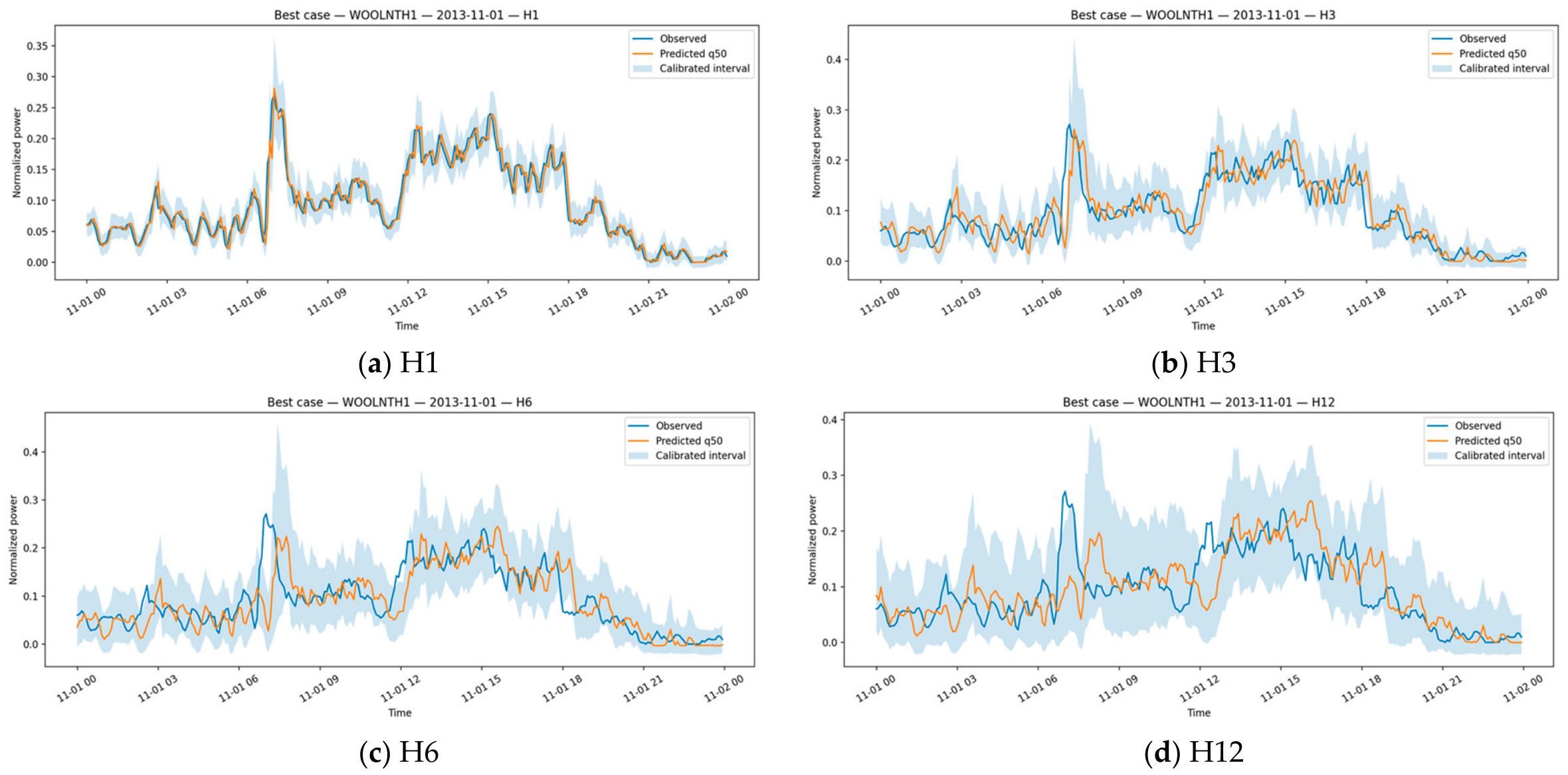
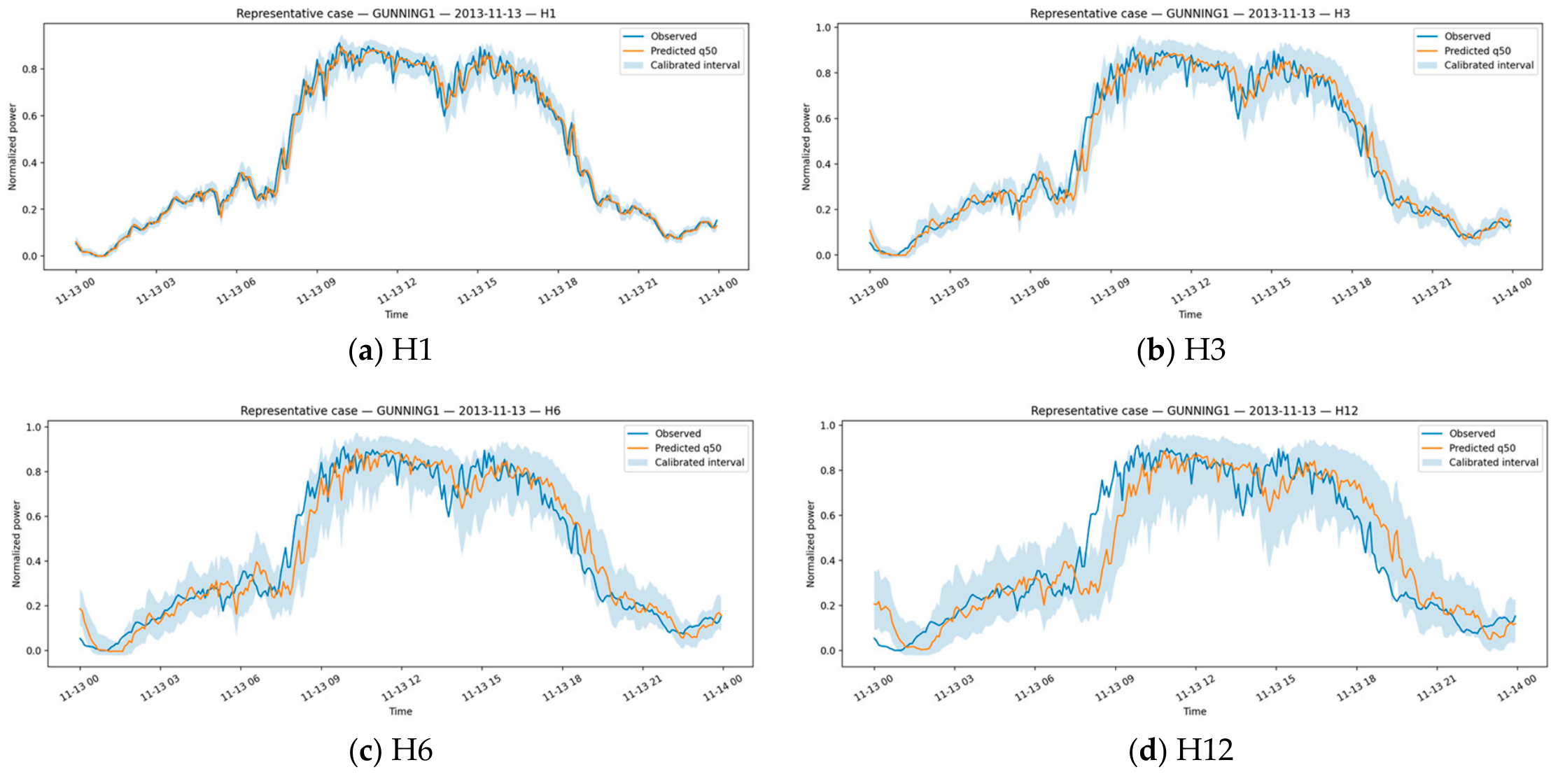
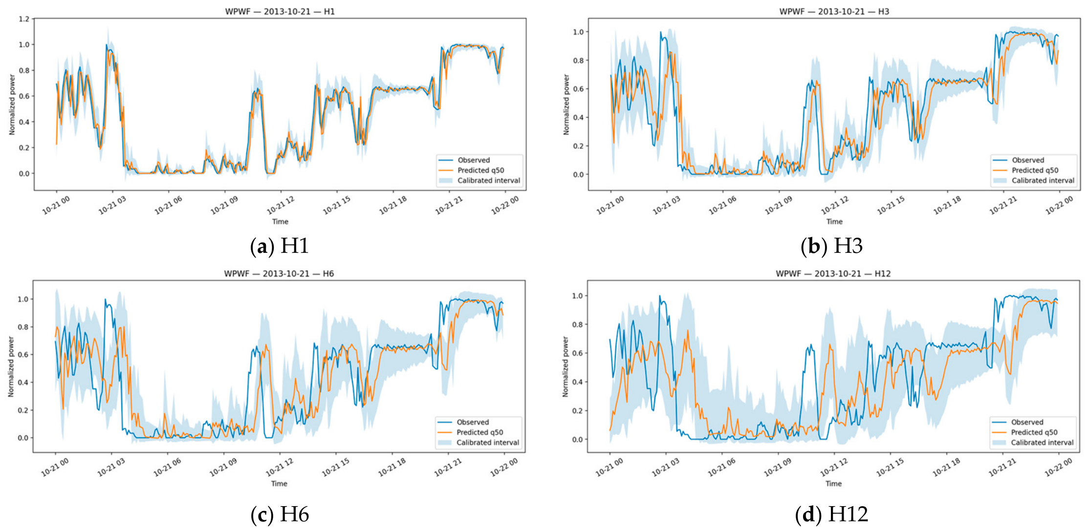
Three typical daily forecasting scenarios were chosen from the test set to offer an operational perspective of the suggested model. A representative scenario on GUNNING1, dated 13 November 2013; a challenging scenario on WPWF, dated 21 October 2013; and a best-case scenario on WOOLNTH1, dated 1 November 2013, represent complementary error regimes. DG-TFT-CQR was assessed at H1, H3, H6, and H12 for each case using the calibrated prediction interval, the median forecast q0.5, and the observed power series. These everyday instances serve as examples. The complete quantitative benchmark shown in Table 3, Table 4, Table 5, Table 6, Table 7, Table 8, Table 9 and Table 10 is not replaced by them.

Figure 5 illustrates that DG-TFT-CQR closely tracks the daily production profile over all horizons in the best-case scenario for WOOLNTH1. As the forecast horizon lengthens, performance only slightly deteriorates. The daily RMSE is still low, rising from 0.0162 at H1 to 0.0328 at H3, 0.0443 at H6, and 0.0493 at H12.

The representative case on GUNNING1, shown in Figure 6a–d, illustrates a more typical daily behavior. The model accurately captures the main upward and downward transitions at H1 and H3, while moderate smoothing effects become visible at H6 and H12. The daily RMSE increases gradually from 0.0377 at H1 to 0.0539 at H3, 0.0732 at H6, and 0.1174 at H12.

The difficult case on WPWF, reported in Figure 7a–d, provides a complementary stress-test perspective. At H1, the model still follows the observed sequence reasonably well, but the mismatch becomes progressively larger at H3, H6, and especially H12. The daily RMSE values rise from 0.0879 at H1 to 0.1567 at H3, 0.2145 at H6, and 0.2554 at H12.

Taken together, these daily examples are fully consistent with the aggregate quantitative results. They show that DG-TFT-CQR provides accurate short-horizon tracking, a progressive and expected degradation with horizon, and uncertainty intervals that broaden under more difficult conditions.

4.8. Complexity and Accuracy–Efficiency Trade-Off

To complement the predictive and probabilistic evaluation, the computational complexity of the compared models was analyzed using the averaged profiling results reported across the available horizons in

Table 11. Average complexity metrics across the available horizons. Lower values indicate lower computational cost.

Model	Avg Params	Avg Training Time (s)	Avg Inference (ms/Sample)	Avg GPU Train (MB)	Avg GPU Inference (MB)	Avg GFLOPs/Sample
CNN-LSTM	58,497	170.63	0.0036	661.48	483.27	0.01438
CNN-LSTM-CQR	100,995	324.89	0.0053	698.02	481.50	0.01479
TSG-Net	364,170	146.50	0.0073	313.62	119.47	0.18196
No_Dynamic_Graph	408,349	773.36	0.0319	4948.51	1157.52	0.09912
DG-TFT-CQR	433,437	1608.11	0.1344	5580.44	533.44	0.09913
DG-TFT-CQR-NoConformal	433,437	1602.86	0.0854	5580.11	1241.32	0.09912

.

The complexity analysis confirms a clear accuracy–efficiency trade-off. DG-TFT-CQR provides the strongest forecasting performance but at the highest computational cost. CNN-LSTM and CNN-LSTM-CQR are much lighter and may therefore be attractive in strongly resource-constrained settings, but they do not match the accuracy and uncertainty quality of the proposed model. TSG-Net offers an efficient alternative with a favorable runtime and memory profile, but its forecasting performance remains below that of DG-TFT-CQR. These findings indicate that the forecasting architecture selected should be based on the operational requirements of the target application. When computational resources are limited, rapid model retraining is required, or inference latency is a major concern, lighter architectures such as CNN-LSTM-CQR or TSG-Net may offer a better cost-performance ratio. On the other hand, applications such as reserve scheduling, grid balancing, renewable energy integration, and uncertainty-aware decision support, in which forecasting errors have significant operational or economic consequences, justify the increased complexity of DG-TFT-CQR. In these cases, the observed improvements in cross-site forecasting robustness, probabilistic reliability, and deterministic accuracy may outweigh the increased computational demands.

DG-TFT-CQR maintained its overall performance advantage over the assessed baselines despite the larger forecasting task, suggesting that the advantages of dynamic graph learning go beyond the scaled-down benchmark setting. However, as more sites are monitored, the computational load inevitably rises.

Overall, the results indicate that DG-TFT-CQR offers the most favorable balance between forecasting performance, uncertainty reliability, and cross-site robustness when predictive quality is prioritized over computational efficiency.

4.9. Robustness Evaluation on the Full 22-Site Benchmark

Although the primary benchmark analysis was conducted on a representative eight-site subset, an additional validation experiment was conducted on the entire 22-site AEMO benchmark to evaluate the proposed framework’s scalability and generalization capabilities. The experiment uses the same training protocol and forecasting settings as the main study.

Table 12. Robustness evaluation on the complete 22-site AEMO benchmark.

Horizon	Model	MAE	RMSE	R2
H1	DG-TFT-CQR	0.024950	0.042753	0.981804
H1	CNN-LSTM-CQR	0.024974	0.042775	0.981786
H1	TFT-CQR	0.025050	0.042838	0.981732
H3	DG-TFT-CQR	0.043417	0.072805	0.947233
H3	TFT-CQR	0.044231	0.074179	0.945222
H3	CNN-LSTM-CQR	0.044188	0.074220	0.945162
H6	DG-TFT-CQR	0.061174	0.099473	0.901498
H6	TFT-CQR	0.062677	0.102079	0.896269
H6	CNN-LSTM-CQR	0.062766	0.102295	0.895829
H12	DG-TFT-CQR	0.088791	0.136157	0.815448
H12	TFT-CQR	0.089028	0.138207	0.809851
H12	CNN-LSTM-CQR	0.089325	0.138658	0.808607

shows the forecasting performance of DG-TFT-CQR, TFT-CQR, and CNN-LSTM-CQR across the entire benchmark. DG-TFT-CQR consistently outperforms other forecasting models across all time horizons. For H1, the model yields MAE/RMSE/R² values of 0.024950/0.042753/0.981804. Similar improvements are seen in H3 (0.043417/0.072805/0.947233), H6 (0.061174/0.099473/0.901498), and H12 (0.088791/0.136157/0.815448).

These findings show that the advantages of dynamic graph learning are preserved as the number of sites increases from eight to twenty-two. The observed improvements thus cannot be attributed solely to the selected subset and are consistent across the entire AEMO benchmark. This additional experiment demonstrates the robustness and scalability of the proposed DG-TFT-CQR framework.

4.10. Robustness Analysis Across Random Seeds

To assess the sensitivity of the forecasting models to stochastic training effects and random initialization, the original experiments with fixed random seed 42 were supplemented with two additional independent runs with random seeds 123 and 456. The proposed DG-TFT-CQR model was tested for robustness against two strong competing baselines: CNN-LSTM-CQR and TSG-Net. All additional runs used the same dataset, data partitions, preprocessing pipeline, model hyperparameters, and training protocol as the main experiments, with only the random seed changed.

Table 13. Multi-seed robustness analysis of forecasting performance based on MAE.

Model	Horizon	Seed 42	Seed 123	Seed 456	Mean MAE	Std	CV (%)
DG-TFT-CQR	H1	0.025490	0.025786	0.025738	0.025671	0.000161	0.63
DG-TFT-CQR	H3	0.037241	0.037296	0.037305	0.037281	0.000035	0.09
DG-TFT-CQR	H6	0.047917	0.047613	0.047699	0.047743	0.000158	0.33
DG-TFT-CQR	H12	0.062891	0.062651	0.062713	0.062752	0.000126	0.20
CNN-LSTM-CQR	H1	0.025841	0.025767	0.025786	0.025798	0.000039	0.15
CNN-LSTM-CQR	H3	0.045811	0.045903	0.045806	0.045840	0.000055	0.12
CNN-LSTM-CQR	H6	0.063550	0.063847	0.063664	0.063687	0.000150	0.24
CNN-LSTM-CQR	H12	0.087915	0.087682	0.087374	0.087657	0.000271	0.31
TSG-Net	H1	0.025940	0.026041	0.026195	0.026059	0.000129	0.50
TSG-Net	H3	0.047009	0.046913	0.047201	0.047041	0.000147	0.31
TSG-Net	H6	0.064892	0.064849	0.064909	0.064883	0.000031	0.05
TSG-Net	H12	0.090857	0.089082	0.091312	0.090417	0.001186	1.31

summarizes the forecasting performance obtained using three random seeds. To quantify performance variability, we calculated the mean MAE, standard deviation, and coefficient of variation (CV) for each forecasting horizon.

The results show that all of the models tested are highly reproducible. For DG-TFT-CQR, the coefficient of variation was less than 0.63% for all forecasting horizons and averaged only 0.31% across the entire evaluation. CNN-LSTM-CQR demonstrated comparable stability (average CV = 0.21%), whereas TSG-Net showed slightly higher variability (average CV = 0.54%), particularly for the longest forecasting horizon.

Importantly, the ranking of competing models remained consistent across random seeds. DG-TFT-CQR consistently produced the highest forecasting accuracy, followed by CNN-LSTM-CQR and TSG-Net. These findings show that the reported forecasting improvements are not due to a favorable random initialization, and they provide further evidence of the proposed framework’s robustness and reproducibility.

5. Discussion

According to the experimental findings, DG-TFT-CQR offers the best overall forecasting framework over the four assessed horizons (H1, H3, H6, and H12). The suggested model is the best for point forecasting in terms of MAE, RMSE, and R2 at each horizon. The more difficult the forecasting task, the greater its advantage. In comparison to the strongest competing baseline, the RMSE improvement rises from 1.36% at H1 to 16.90% at H3, 20.66% at H6, and 22.32% at H12. This demonstrates that when temporal uncertainty rises, the suggested architecture maintains predictive accuracy more successfully than the compared baselines.

A similar pattern appears in the probabilistic results. DG-TFT-CQR keeps relatively narrow intervals and maintains empirical coverage close to the nominal 90% target across all four horizons. By combining competitive interval sharpness and reliable empirical coverage, the suggested model displays the most balanced uncertainty-aware behavior rather than being consistently better for all probabilistic metrics. This distinction is important because, while conformal calibration increases reliability, it may also cause prediction intervals to widen, which can have an impact on interval-score efficiency over specific time periods. This balance is important from an operational standpoint because uncertainty intervals need to continue to be useful as the forecast horizon lengthens. They shouldn’t get too broad to allow for sensible choices.

The ablation and statistical results need careful interpretation. DG-TFT-CQR should not be described as uniformly superior across every metric and horizon. A more accurate conclusion is that it is the strongest balanced framework in the benchmark. Its advantage is clearest at H1 and H12, where both descriptive and statistical evidence support the proposed model. Results at H3 and H6 are more mixed, especially in pairwise comparisons with CNN-LSTM-CQR and NoConformal. In these cases, some point-wise or raw probabilistic metrics become less decisive or may favor the baseline.

Particularly helpful for comprehending split conformal calibration is the comparison with NoConformal. DG-TFT-CQR and NoConformal generate identical median forecasts and raw quantile predictions in the exported outputs starting with H3. This indicates that the conformal calibration stage is the only source of the observed differences. The conformalized version becomes more conservative but increases reliability in this situation.

However, increased conservatism may reduce interval-score efficiency and calibrated pinball performance over medium and long time horizons. As a result, conformal calibration should not be regarded as uniformly superior across all probabilistic measures. Its primary contribution is improved uncertainty reliability, rather than a systematic improvement in interval sharpness or efficiency.

The site-wise analysis further supports the benchmark interpretation. DG-TFT-CQR achieves the lowest RMSE on all eight wind farms. This shows that the gain is not caused by one or two favorable sites. The model generalizes well across both easier and more difficult locations, which supports its robustness in the reduced multi-site setting considered in this study.

Furthermore, the multi-seed robustness analysis confirms that these gains remain stable across independent training runs, with DG-TFT-CQR achieving an average coefficient of variation of only 0.31% across the evaluated horizons. This low variability indicates that the reported gains are not the result of a favorable random initialization, but reflect a stable training behavior of the proposed architecture.

6. Limitations and Scope of Interpretation

Although the empirical findings are encouraging, they should be interpreted within the scope of the present experimental design.

First, the primary benchmark analysis is performed on a representative eight-site subset of the AEMO dataset, enabling detailed site-specific probabilistic calibration, ablation, and complexity analyses. Although an additional validation experiment on the entire 22-site benchmark confirms the proposed framework’s scalability, further validation on independent datasets, across different geographical regions, and in alternative operational forecasting settings would provide stronger evidence of generalizability.

Second, the input configuration used in this study is intentionally restricted to historical power measurements, production-derived temporal variables, static site descriptors, and deterministic calendar encodings. The current experimental setting excludes meteorological observations and numerical weather prediction variables such as wind speed, wind direction, temperature, pressure, and forecast weather fields. This option allows the evaluation to concentrate on the contributions of the proposed dynamic graph, temporal fusion, quantile regression, and conformal calibration components in a controlled historical-power-based environment. However, it also limits the operational interpretation of the results, especially for longer short-term horizons like H6 and H12, where meteorological and NWP data can provide significant predictive value. As a result, the proposed framework should be viewed as a historical-power-based short-term wind power forecasting model, rather than a fully operational forecasting system that incorporates meteorological or NWP inputs. Future work will broaden the input space by incorporating meteorological observations and NWP forecast fields to test the model under more realistic operational forecasting scenarios.

Third, the conformal calibration stage is implemented through a pooled split conformal strategy. This choice provides a simple and robust reliability-oriented post- processing layer, but it may not fully capture horizon-specific or site-specific heterogeneity in predictive uncertainty. More localized calibration procedures may yield a different calibration–sharpness trade-off.

Fourth, although the proposed framework inherits interpretable components from the TFT design, the present manuscript focuses primarily on predictive evaluation. A deeper interpretability analysis, including variable importance patterns, temporal attention behavior, and dynamic graph structure analysis, is left for future work. As a result, the paper demonstrates the predictive usefulness of these mechanisms more strongly than their explanatory behavior.

Finally, the benchmark emphasizes experimental consistency across models rather than exhaustive architecture-specific tuning for every competing baseline. This makes the comparison controlled and coherent, but it also means that the reported results should be interpreted as evidence under a unified evaluation framework rather than as individually optimized best-case performance for every model family.

7. Conclusions

This paper proposed DG-TFT-CQR, a global multi-site probabilistic wind power forecasting framework that integrates static site conditioning, conditional variable selection, dynamic graph learning, encoder–decoder temporal modeling, interpretable temporal attention, quantile forecasting, and post hoc split conformal calibration. The model was evaluated under four distinct forecasting settings, namely H1, H3, H6, and H12, on a representative eight-site subset of the AEMO wind power benchmark. Although the primary benchmark was conducted on this representative eight-site subset, an additional validation experiment on the full 22-site AEMO benchmark was also performed to assess the robustness of the observed conclusions further.

The key findings can be summarized as follows. First, DG-TFT-CQR achieved the strongest overall point-forecasting performance across the four horizons, with MAE/RMSE/R² values of 0.025490/0.043186/0.980096 at H1, 0.037241/0.062569/0.958221 at H3, 0.047917/0.079747/0.932133 at H6, and 0.062891/0.102751/0.887340 at H12. Second, it also delivered the most balanced probabilistic performance, with pinball loss/PICP/PINAW/interval score of 0.008289/0.887562/0.094770/0.156348 at H1, 0.012120/0.889894/0.138525/0.229642 at H3, 0.015623/0.891503/0.179016/0.294191 at H6, and 0.020478/0.891706/0.236781/0.386924 at H12. Third, the advantages of the proposed framework were observed across the eight wind farms and were further supported by the ablation results, which showed that the complete architecture remained the best-performing overall configuration across the evaluated horizons.

At the same time, the results suggest that DG-TFT-CQR should be interpreted as the strongest overall trade-off rather than as a method that dominates all alternatives on every single criterion. This conclusion is particularly well supported at H1 and H12, whereas H3 and H6 should be interpreted more cautiously as mixed regimes. The comparison with NoConformal further shows that conformal calibration improves reliability, but may reduce some interval-efficiency metrics beyond H1. Therefore, the practical value of DG-TFT-CQR lies in its ability to provide a robust balance between point accuracy, probabilistic reliability, and operational usefulness.

Although DG-TFT-CQR introduces higher computational requirements than several competing baselines, the empirical results indicate that the additional complexity is justified in forecasting environments where both predictive accuracy and uncertainty quantification are critical. Future work should therefore focus on broader validation settings, richer exogenous predictors, and improved calibration strategies that better preserve interval sharpness at medium and long horizons. Overall, the present study shows that DG-TFT-CQR is a robust and practically meaningful forecasting framework for uncertainty-aware multi-site wind power prediction, whose principal strength lies in jointly addressing forecasting accuracy and uncertainty reliability across diverse forecasting settings.