Standardized Precipitation Index Forecasting Comparison Using Transformer Models

Highlights

What are the main findings?

• PatchTST achieved the lowest RMSE in three of the four climatic regions of Zacatecas and statistically outperformed the other Transformer models according to the Diebold-Mariano test (p < 0.05).
• The Vanilla Transformer showed superior performance in the Highlands region, demonstrating that model accuracy is strongly influenced by regional climatic variability.

What are the implication of the main findings?

• The results highlight the importance of region-specific model selection for operational drought forecasting in semi-arid environments.
• Transformer-based models, particularly PatchTST, offer a robust and efficient tool to strengthen the Mexico Drought Monitor operated by CONAGUA and improve early warning systems under climate change.

Abstract

Accurate long-horizon drought forecasting is essential for water resource management and early warning systems in semi-arid regions. This study evaluates five state-of-the-art Transformer architectures—Vanilla Transformer, Informer, Autoformer, Temporal Fusion Transformer (TFT), and PatchTST—for 24-month forecasting of the Standardized Precipitation Index (SPI-12) across four climatically homogeneous regions of Zacatecas, Mexico (Semi-arid, Highlands, Mountains, and Canyons). Models were trained on monthly precipitation data from 1965–2022 and evaluated on an independent test period (2023–2024) using MAE, RMSE, Pearson correlation, and the Diebold–Mariano test. The results show that PatchTST achieved the best overall performance in three of the four regions, significantly outperforming the other models in most cases. The Vanilla Transformer performed best in the less variable Highlands region. These findings demonstrate that the model’s suitability is strongly dependent on regional climatic characteristics. PatchTST’s patch-based approach proved particularly effective for capturing complex temporal dependencies in highly variable semi-arid environments. This study highlights the potential of Transformer architectures, especially PatchTST, to improve long-horizon SPI forecasting and strengthen operational drought monitoring systems in water-scarce regions.

1. Introduction

Climate change is increasingly recognized as a major driver of alterations in global precipitation patterns, leading to more frequent and severe extreme events such as prolonged droughts and intense rainfall episodes [1,2]. In arid and semi-arid regions, these changes pose significant threats to water security, agricultural productivity, and socio-economic stability [3,4]. Accurate forecasting of drought conditions is therefore essential for proactive water resource management and the development of early warning systems, particularly in vulnerable areas such as north-central Mexico.

Among the various drought monitoring tools available, the Standardized Precipitation Index (SPI) has become one of the most widely adopted indicators worldwide due to its simplicity, flexibility across multiple timescales, and reliance solely on precipitation records [5,6]. The SPI quantifies the deviation of observed precipitation from the long-term climatological mean, enabling consistent comparison of drought severity across space and time. In Mexico, the SPI has been successfully applied to delineate homogeneous precipitation zones and to characterize regional drought dynamics, particularly in states such as Zacatecas [7].

Over the past decade, machine learning approaches have demonstrated strong potential for SPI forecasting. Traditional statistical models such as ARIMA and SARIMA often struggle with the nonlinear and non-stationary nature of precipitation time series [8,9]. In response, artificial neural network (ANN) models have been increasingly adopted, with promising results reported using Multilayer Perceptron (MLP) networks [10], Nonlinear Autoregressive Networks with Exogenous Inputs (NARX) [11], Neural Hierarchical Interpolation for Time Series Forecasting (N-HiTS) [12], and automated machine learning (AutoML) frameworks [13]. Complementary regional studies have further confirmed the increasing frequency and severity of drought events in central Zacatecas using ANN-based approaches [14] and climate variability indices [15].

Despite these advances, conventional ANN and recurrent architectures still face limitations in capturing long-range dependencies and complex seasonal patterns that characterize monthly SPI series. Recurrent models, in particular, process sequences sequentially, which can hinder their ability to model multi-scale variability effectively.

Recent breakthroughs in deep learning have introduced Transformer-based models as a powerful alternative. Architectures such as PatchTST [16], Autoformer [17], Informer [9], and Temporal Fusion Transformer (TFT) [18] leverage self-attention mechanisms, patching strategies, and decomposition techniques to outperform recurrent networks in long-horizon forecasting tasks [19,20,21]. However, their application in hydroclimatology, especially for SPI forecasting in Latin America and Mexico remains limited [21,22].

Building on a progressive research line that includes MLP [10], NARX [11], N-HiTS [12], and AutoML approaches [13], the present study represents the next methodological step by evaluating five state-of-the-art Transformer architectures—Vanilla Transformer, Informer, Autoformer, PatchTST, and TFT—for monthly SPI-12 forecasting. The analysis focuses on four climatically homogeneous regions of Zacatecas (Semi-arid, Highlands, Mountains, and Canyons) using long-term time series and a 24-month forecast horizon. Model performance is assessed through MAE, RMSE, Pearson correlation, and the Diebold–Mariano test.

The main contributions of this study are threefold: (i) a comprehensive comparison of multiple Transformer architectures for long-horizon SPI forecasting in semi-arid conditions; (ii) an evaluation of model performance across distinct climatic regions, highlighting the role of regional variability; and (iii) an extension of previous ANN-based work by demonstrating the effectiveness of direct multi-step SPI forecasting with attention-based models, supported by rigorous statistical validation.

The remainder of this paper is organized as follows. Section 2 describes the study area, data, and methodology. Section 3 presents the forecasting results. Section 4 discusses the main findings and their operational implications. Finally, Section 5 summarizes the conclusions and outlines directions for future research.

2. Materials and Methods

2.1. Study Region and Datasets

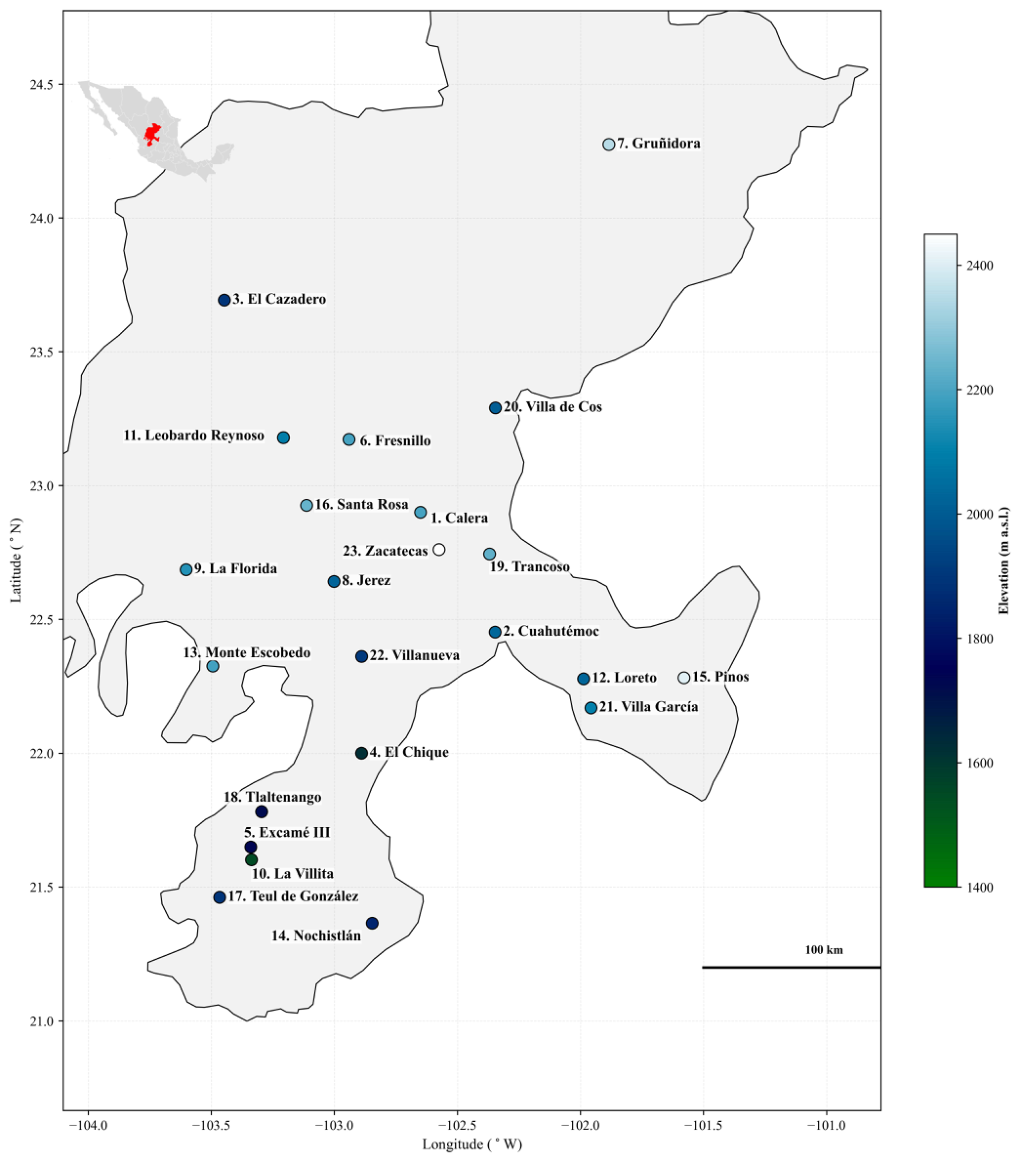
This study used monthly rainfall time series collected from weather stations across the state of Zacatecas, Mexico (Figure 1).

Data were obtained from the National Meteorological Service network and cover the period 1965–2022. Prior to analysis, a comprehensive quality control was performed to remove outliers, missing values, and erroneous records. Stations with incomplete records or evident data gaps were excluded, resulting in 23 stations with continuous series. The cleaned precipitation data were then used to compute the Standardized Precipitation Index time series.

2.2. Standardized Precipitation Index

The Standardized Precipitation Index is a widely recognized drought indicator that quantifies the deviation of observed precipitation from the long-term climatological mean [5]. It is calculated solely from precipitation records and allows consistent comparison across regions and timescales. Following McKee et al. [5] and the SPEI package implementation, monthly rainfall was fitted to a gamma distribution:

$$g\left(x\right)={\displaystyle \frac{1}{{\beta }^{\alpha }\mathsf{\Gamma }\left(\alpha \right)}}{x}^{\alpha -1}{e}^{{\displaystyle \frac{-x}{\beta }}},$$

(1)

for $x>0$.

Where $g\left(x\right)$ is the probability density function, $\alpha$ is the shape parameter $(\alpha >0)$, $\beta$ is a scale parameter $(\beta >0)$, and

$$\mathsf{\Gamma }\left(\alpha \right)={\int }_0^{\infty }{y}^{\alpha -1}{e}^{-y}dy.$$

(2)

where $\mathsf{\Gamma }\left(\alpha \right)$ is the gamma function.

The parameters $\alpha$ and $\beta$ are estimated as follows:

$$\alpha ={\displaystyle \frac{1}{4A}}\left(1+\sqrt{1+{\displaystyle \frac{4A}{3}}}\right)$$

(3)

$$\beta ={\displaystyle \frac{\overline{x}}{A}}$$

(4)

$$A=ln\left(\overline{x}\right)-{\displaystyle \frac{\sum ln\left(\overline{x}\right)}{n}}$$

(5)

where n is the number of precipitation observations and $\overline{x}$ is the arithmetic mean over the time scale of interest. A cumulative probability $G\left(x\right)$ of an observed amount of rainfall in a given month and time scale (if $\alpha$ and $\beta$ estimators were used to integrate the probability density function with respect to x) is obtained as follows:

$$G\left(x\right)={\int }_0^{x}g\left(x\right)dx={\displaystyle \frac{1}{{\beta }^{-\overline{\alpha }}\mathsf{\Gamma }\left(\overline{\alpha }\right)}}{\int }_0^x{x}^{\overline{\alpha }}{e}^{{\displaystyle \frac{\overline{x}}{\overline{\beta }}}}dx$$

(6)

When substituting t for ${\displaystyle \frac{\overline{x}}{\overline{\beta }}}$ in the previous equation, it results in the incomplete gamma function:

$$G\left(x\right)={\displaystyle \frac{1}{\mathsf{\Gamma }\left(\overline{\alpha }\right)}}{\int }_0^x{t}^{\overline{\alpha }-1}{e}^{-t}dt$$

(7)

Nevertheless, the gamma distribution function is undefined for $x=0$ and $q=P(x=0)>0$; where $P(x=0)$ is the probability of zero precipitation. Hence, the actual probability of non-exceedance $H\left(x\right)$ should be calculated as follows:

$$H\left(x\right)=q+\left(1-q\right)G\left(x\right)$$

(8)

where $H\left(x\right)$ is the actual probability of non-exceedance and q the probability of $x=0$. If m is zero in a sample of size n, then q is estimated as

$$q={\displaystyle \frac{m}{n}}$$

(9)

Finally, $H\left(x\right)$ is transformed to a standard normal variable to obtain the SPI value.

The SPI values derived can be categorized according to their magnitude. Negative values reflect conditions that are dryer than the average, whereas positive values denote conditions that are wetter than the average.

Table 1. Classification of drought/wetness conditions according to SPI values (McKee et al., 1993) [5].

Region	PP (mm)
≥ 2.0	Extremely Wet
1.5 to 1.99	Severely wet
1.0 to 1.49	Moderately wet
−0.99 to 0.99	Near normal
−1.49 to −0.99	Moderately dry
−1.99 to −1.49	Severely dry
≤−2.0	Extremely dry

provides a classification of SPI values ranging from “extremely dry” to “extremely wet,” with intermediate categories that reflect different levels of drought or wetness, including moderate to severe conditions.

The SPI calculations incorporate multiple time scales due to the impact of precipitation variability on different components of the hydrological cycle [6]. Specifically, SPI values calculated over a 3-month duration provide insight into short- to medium-term moisture conditions, whereas 6-month SPI values are particularly relevant for assessing drought conditions that have implications for agricultural practices. In addition, the 12-month SPI values serve to assess drought effects that are significant for aquifer health and groundwater levels.

This research involved the computation of SPI values across a 12- month time scale, utilizing R software version 4.4.1 [23] in conjunction with the ‘SPEI’ package version 1.8.1 [24].

2.3. Regionalization of the Study Area

The study area was divided into four climatically homogeneous regions using hierarchical cluster analysis. Monthly SPI-12 time series from the 23 weather stations (1965–2022) were used as input variables. Ward’s minimum variance method combined with Minkowski distance was applied as the agglomeration criterion.

Prior to clustering, a Pearson correlation matrix was computed among all stations to identify potential redundant information. Most paired correlations were below 0.75, with 0.89 being the highest observed value between stations 5 (Excame III) and 10 (La Villita). It is worth noting that station Excame III is situated immediately adjacent to a major reservoir (the third largest dam in the state of Zacatecas). This massive body of water exerts a distinct microclimatic regulation effect via localized evaporation and thermal stabilization, contrasting with Station La Villita, which lacks this direct hydrological influence. For this reason, this pair of stations was retained because it captures complementary microclimatic signals due to differences in elevation. This is clearly illustrated in Figure 1, where the altitude colormap functions as a simplified digital elevation model.

Following the identification of the four climatically homogeneous clusters, the representative regional SPI-12 time series were synthesized using the arithmetic mean of the individual monthly SPI-12 values from all stations belonging to each respective zone. While the arithmetic mean successfully preserves the shared macro-climatic trend of the cluster, it inherently acts as a statistical filter that smooths out extreme localized variance. In high-variability regions characterized by complex topography, such as the Canyons, this smoothing effect can suppress fine-grained local fluctuations, contributing to delayed temporal tracking and systematic model biases during rapid climatic shifts.

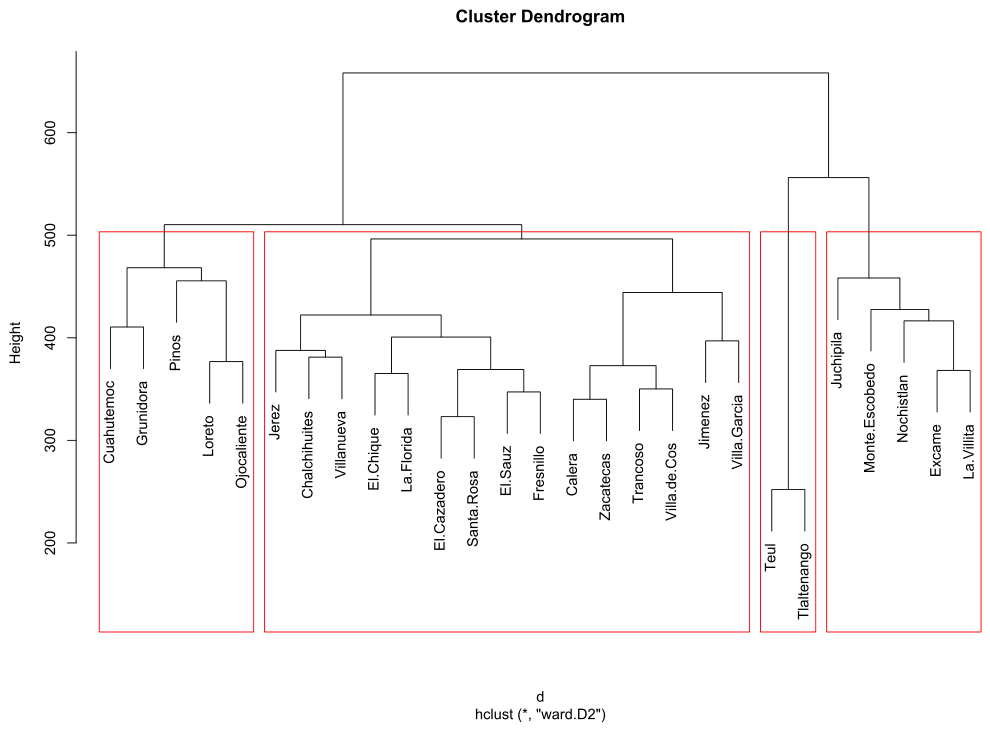
The resulting clusters align well with the spatial distribution of the pluvial regime. The dendrogram supported the selection of four distinct groups corresponding to the regions denominated Semi-arid, Highlands, Mountains, and Canyons. These regions exhibit markedly different precipitation regimes and variability levels, justifying separate model evaluation.

2.4. Neural Time Series Forecasting

Machine learning methods have proven effective for modeling nonlinear and non-stationary climate time series [25,26]. In this study, five state-of-the-art Transformer architectures were implemented using the NeuralForecast library (version 1.7.0) [27]: Vanilla Transformer, Informer, Autoformer, Temporal Fusion Transformer (TFT), and PatchTST.

2.4.1. Transformer Architectures and Model Descriptions

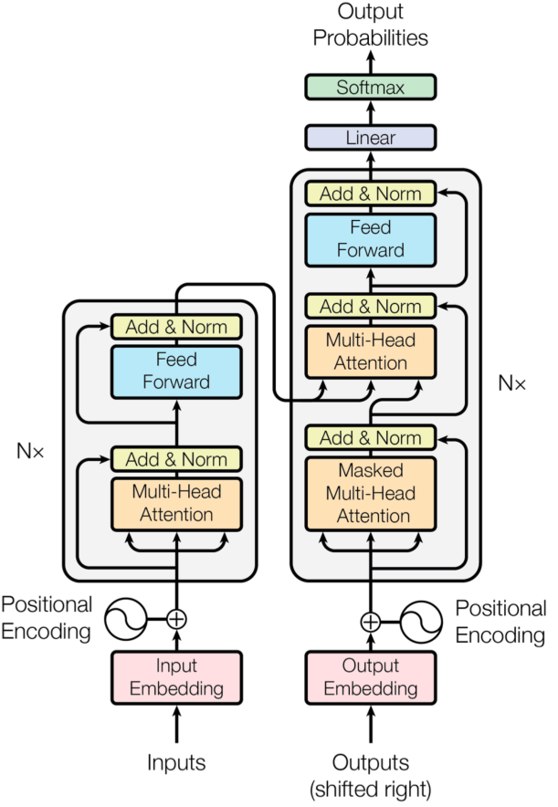
Transformer-based models were implemented in this study to capture the complex temporal dependencies of the SPI-12 series. A general structural schematic of the operational framework and data processing pipeline for these architectures is presented in Figure 2. To enhance the clarity of our comparative analysis and address the architectural evolution across variants, the internal mechanisms unique to each evaluated configuration are detailed below:

Vanilla Transformer

The standard Transformer originally proposed by [28] for natural language processing, relies entirely on the classical Multi-Head Attention mechanism, which computes global pairwise dependencies across the entire sequence. While highly effective for capturing multi-scale seasonal contexts, its quadratic computational and memory complexity, $\mathcal{O}\left(L^2\right)$, can pose challenges when training on extensive climate records.

Informer

Designed specifically for long-horizon forecasting, the Informer introduces the ProbSparse self-attention mechanism, which selectively computes attention scores only for the dominant “active” queries. By optimizing the sequence processing to $\mathcal{O}(LlnL)$ complexity and utilizing a distilling operation to reduce temporal dimensions, it mitigates computational overhead while remaining robust to the high variability of semi-arid climate data.

Autoformer

This architecture replaces pointwise self-attention with an Auto-Correlation mechanism based on the Wiener-Khinchin theorem. By computing series-level dependencies in the frequency domain via Fast Fourier Transforms, Autoformer focuses on multi-scale periodic patterns. Additionally, it natively integrates a deep series decomposition block within its hidden layers to isolate trend-cyclical components from seasonal fluctuations, making it highly suitable for long-term hydrological indices.

Temporal Fusion Transformer

Specialized for multi-horizon forecasting, the TFT incorporates Gated Residual Networks and Variable Selection Networks to automatically identify and weigh the most relevant input features. It leverages self-attention layers strictly to capture long-term temporal relationships while utilizing specialized LSTM-based components for localized processing, providing an interpretable framework for tracking climatic transitions.

PatchTST

Unlike traditional models that process individual time steps, PatchTST aggregates sequential monthly records into continuous, overlapping patches. This patch-based approach preserves localized semantic information and reduces the attention matrix sequence length from L to approximately $L/P$ (where P is patch length), shifting the complexity to $\mathcal{O}\left({(L/P)}^2\right)$. Furthermore, it employs a channel-independence strategy where each regional time series is modeled as an independent univariate channel, significantly enhancing generalization and preventing cross-feature noise during extreme drought horizons.

Detailed mathematical formulations of the core multi-head self-attention layout, positional encodings, and the precise matrix equations for these architectural modifications are provided in Appendix A.

FEDformer was excluded from the final comparative analysis due to specific convergence failures when processing noisy univariate series. This architecture relies on an attention mechanism computed over compact wavelets or frequency modes via Fourier transforms. When applied to our specific dataset (a normalized, univariate climatic index characterized by high stochastic noise and a lack of smooth continuous periodic transitions), the model suffered from extreme validation loss oscillations and eventual gradient explosion. The architecture failed to isolate a stable, dominant set of compact frequency components, leading to a complete failure to converge during early epochs, which highlights its operational boundaries when processing high-frequency, noisy univariate meteorological inputs without multivariable context.

2.4.2. Model Configuration and Hyperparameter Optimization

All models were configured for direct multi-step forecasting with a lookback window (input_size) and forecast horizon (h) both equal to 24 months. This configuration is consistent with the monthly resolution of the SPI-12 series and the operational requirements of drought early warning systems.

A sensitivity analysis was performed by varying the number of training epochs from 50 to 400 (in increments of 50), while keeping all other hyperparameters constant: batch size = 16, loss function = Mean Absolute Error (MAE), random seed = 42 (for reproducibility), and Adam optimizer with default learning rate. Validation performance (RMSE) stabilized at 250 epochs, after which marginal improvements were observed together with increased computational cost and risk of overfitting. Therefore, 250 epochs were selected as the final training configuration for all models and regions.

The models were trained using a chronological 80/20 train-validation split of the 1965–2022 period to preserve temporal order and avoid data leakage. Specifically, the historical data was partitioned into a training set spanning 1965–2011 and a validation set spanning 2012–2022. This validation timeline is highly strategic for the experimental design, as it encompasses major multi-scale climatic anomalies in Mexico (including the historic severe multi-state drought of 2011–2012 and subsequent intense wet recovery phases) thereby providing a highly rigorous and realistic stress-test environment for hyperparameter optimization and model selection.

Table 2. Main hyperparameters used for each Transformer model. Patch length and stride are specific to the PatchTST architecture, while the other models do not use a patching strategy.

Model	Patch Length	Stride	d_Model	Heads	Learning Rate
Vanilla Transformer	-	-	512	8	1 $\times {10}^{-4}$
Informer	-	-	512	8	1 $\times {10}^{-4}$
Autoformer	-	-	512	8	1 $\times {10}^{-4}$
TFT	-	-	512	8	1 $\times {10}^{-4}$
PatchTST	16	8	128	8	1 $\times {10}^{-4}$

summarizes the main hyperparameters used for each model.

2.4.3. Evaluation Metrics

Model performance was assessed using three complementary metrics: Mean Absolute Error (MAE), Root Mean Square Error (RMSE), and Pearson correlation coefficient (r). These metrics were calculated on the independent test set (January 2023–December 2024). In addition, the Diebold–Mariano test was applied to statistically compare the predictive accuracy of the different models. Squared errors were used as the loss function for the test. A p-value < 0.05 was considered statistically significant.

2.4.4. Limitations of the Current Approach and Future Extensions

Although the present study provides a comprehensive comparison among state-of-the-art Transformer architectures, certain limitations should be acknowledged. First, classical statistical benchmarks such as ARIMA or SARIMA were not included. This decision was made to maintain focus on modern deep learning approaches. Future work will incorporate these traditional methods as baselines.

Second, the models implemented in this study are univariate. While this facilitates interpretation and computational efficiency, it restricts the incorporation of large-scale climate drivers such as the El Niño-Southern Oscillation (ENSO).

Finally, the current evaluation is based solely on point forecasts. Extending the analysis to probabilistic forecasting (e.g., quantile outputs from TFT or ensemble strategies in PatchTST) would provide uncertainty estimates that are highly valuable for operational drought risk management.

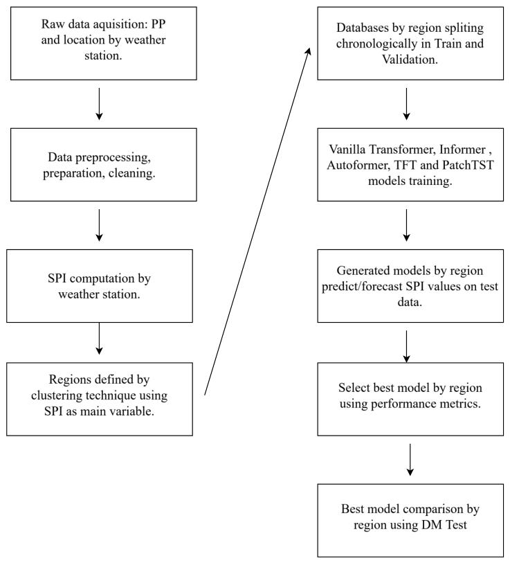
The data flow of the whole process is shown in Figure 3.

3. Results

3.1. Cluster Analysis

The dataset initially comprised 23 distinct rainfall time series, from which SPI-12 time series were derived. Hierarchical cluster analysis was applied to the complete SPI dataset, resulting in the identification of four climatically homogeneous regions—Semi-arid, Highlands, Mountains, and Canyons—characterized by similar SPI patterns (Figure 4). The regional SPI time series for these four areas were subsequently used as inputs for predictive modeling with Vanilla Transformer, Informer, Autoformer, TFT, and PatchTST architectures.

3.2. Descriptive Statistics of Input Predictors

Table 3. Descriptive statistics of monthly precipitation (PP) by region (1965–2022).

Region	Mean	Max	SD
Semi-arid	39.300	325.317	44.119
Highlands	38.757	299.900	44.647
Mountains	56.438	355.880	66.838
Canyons	65.589	347.501	81.612

and

Table 4. Descriptive statistics of Standardized Precipitation Index (SPI) by region based on observed time series (1965–2022).

Region	Min	Mean	Max	SD
Semi-arid	−2.255	0.022	2.148	0.787
Highlands	−1.994	0.032	1.966	0.764
Mountains	−2.307	−0.090	2.214	0.800
Canyons	−3.549	0.042	2.531	0.952

summarize the descriptive statistics for monthly precipitation (PP) and Standardized Precipitation Index (SPI) across the four climatic regions of Zacatecas, based on observed time series from 1965 to 2022. The Semi-arid region showed the lowest mean PP (39.300 mm) and SPI (0.022), with maximum values of 325.317 mm and 2.148, respectively. This region also presented high variability (SD = 44.119 mm for PP and 0.787 for SPI). The Highlands region exhibited a similar low mean PP (38.757 mm) but a slightly higher mean SPI (0.032), with SD values of 44.647 mm and 0.764.

In contrast, the Mountains and Canyons regions displayed higher precipitation levels, with mean PP of 56.438 mm and 65.589 mm, and mean SPI values of −0.090 and 0.042, respectively. These regions showed greater variability (SD = 66.838 mm and 81.612 mm for PP; 0.800 and 0.952 for SPI). Minimum SPI values ranged from −1.994 to −3.549 across regions, highlighting severe drought episodes, while maximum values (1.966 to 2.531) indicated periods of above-average wetness. These statistics confirm the diverse climatic regimes in Zacatecas and justify the regional clustering approach for model evaluation.

3.3. Sensitivity Analysis on Training Epochs

A sensitivity analysis was conducted by varying the number of training epochs from 50 to 400 (in increments of 50), while keeping all other hyperparameters constant. Validation performance (RMSE) improved progressively up to 250 epochs, after which gains became marginal while computational cost and risk of overfitting increased. PatchTST maintained strong performance beyond 200 epochs in three regions, while Vanilla Transformer performed best in the Highlands. Therefore, 250 epochs were selected as the optimal configuration for all models and regions.

3.4. Historical Metrics (One-Step-Ahead Forecasting)

Table 5. Summary of model performance metrics by region based on SPI observed time series (1965–2022).

Region	Model	MAE	RMSE
Semi-arid	Vanilla Transformer	0.433	0.576
	Informer	0.365	0.524
	Autoformer	0.486	0.636
	TFT	0.349	0.498
	PatchTST	0.407	0.560
Highlands	Vanilla Transformer	0.460	0.606
	Informer	0.398	0.571
	Autoformer	0.716	0.905
	TFT	0.442	0.699
	PatchTST	0.543	0.734
Mountains	Vanilla Transformer	0.385	0.486
	Informer	0.332	0.445
	Autoformer	0.408	0.525
	TFT	0.359	0.583
	PatchTST	0.336	0.458
Canyons	Vanilla Transformer	0.592	0.854
	Informer	0.523	0.815
	Autoformer	0.776	1.012
	TFT	0.412	0.637
	PatchTST	0.603	0.887

summarizes the Mean Absolute Error (MAE) and Root Mean Square Error (RMSE) for the five Transformer models in one-step-ahead forecasting on the historical data (1965–2022). In the Semi-arid region, TFT achieved the lowest errors (MAE = 0.349, RMSE = 0.498), followed by Informer and PatchTST. In the Highlands, Informer obtained the best performance (MAE = 0.398, RMSE = 0.571). Similar patterns were observed in the Mountains and Canyons regions, where TFT and Informer generally performed well. Overall, TFT and Informer showed strong in-sample performance, particularly in regions with lower variability.

3.5. Test Metrics (24-Month Out-of-Sample Forecasting)

Table 6. Summary of model performance metrics by region based on SPI test time series (2023–2024).

Region	Model	MAE	RMSE	r
Semi-arid	Vanilla Transformer	1.132	1.256	0.357
	Informer	1.378	1.538	0.299
	Autoformer	0.968	1.082	0.239
	TFT	0.902	1.039	−0.507
	PatchTST	0.554	0.615	0.397
Highlands	Vanilla Transformer	0.432	0.536	0.790
	Informer	0.765	0.898	−0.264
	Autoformer	0.726	0.877	0.463
	TFT	0.568	0.703	−0.498
	PatchTST	0.583	0.691	0.080
Mountains	Vanilla Transformer	0.498	0.619	0.218
	Informer	0.561	0.703	−0.092
	Autoformer	0.340	0.491	0.153
	TFT	0.417	0.604	0.162
	PatchTST	0.317	0.425	0.362
Canyons	Vanilla Transformer	1.407	1.718	−0.453
	Informer	1.268	1.511	0.529
	Autoformer	1.205	1.530	−0.325
	TFT	1.205	1.406	−0.032
	PatchTST	0.802	1.053	0.508

presents the MAE, RMSE, and Pearson correlation coefficient (r) for the 24-month out-of-sample test period (2023–2024). PatchTST emerged as the best model in three regions: Semi-arid (MAE = 0.554, RMSE = 0.615, r = 0.397), Mountains (MAE = 0.317, RMSE = 0.425, r = 0.362), and Canyons (MAE = 0.802, RMSE = 1.053, r = 0.508). Vanilla Transformer performed best in the Highlands (MAE = 0.432, RMSE = 0.536, r = 0.790). These results highlight PatchTST’s superior generalization capability for long-horizon SPI forecasting in variable environments.

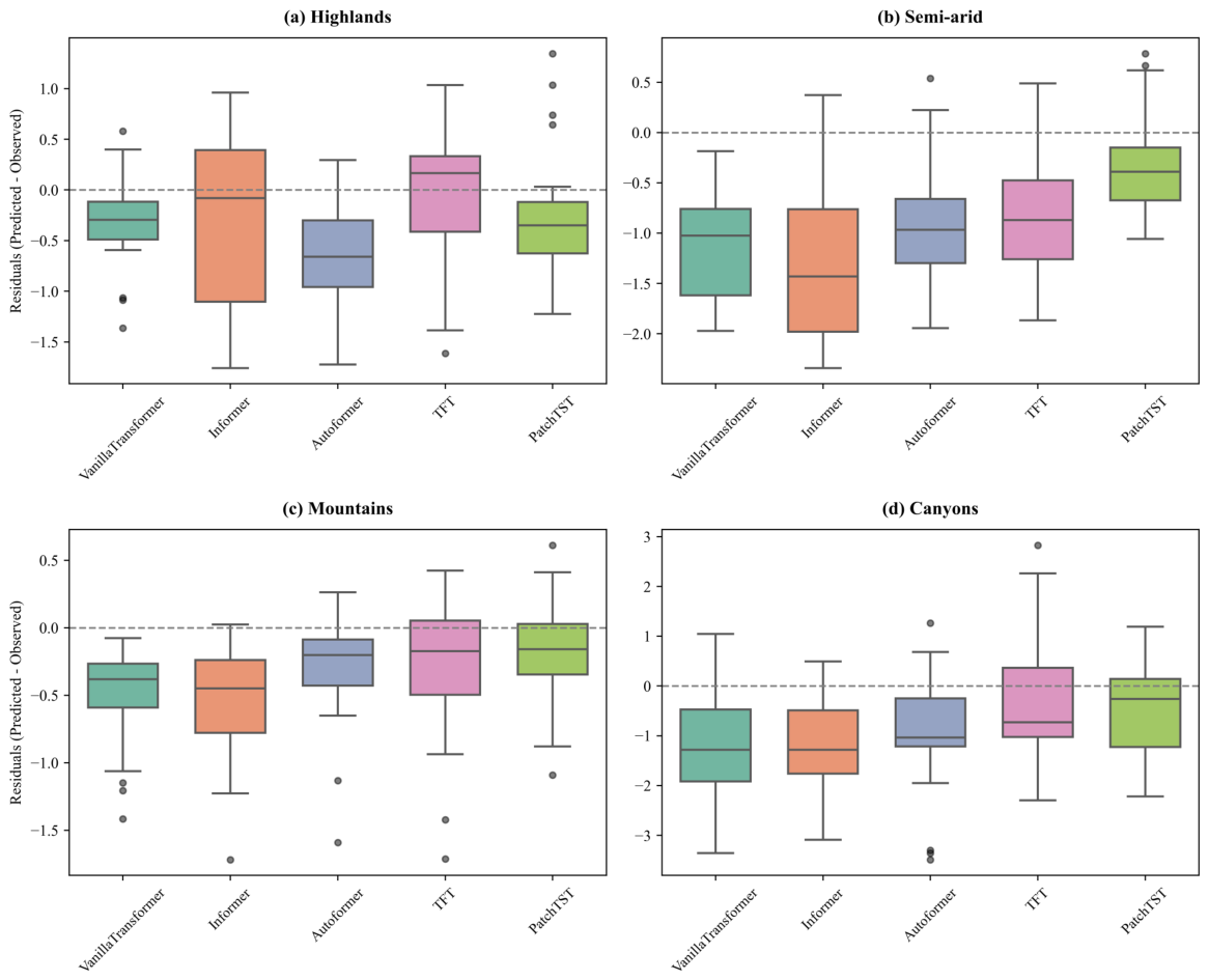
Additionally, a systematic negative bias (dry bias) was observed in several regions, particularly in Canyons, where the median residual was consistently below zero across most models. This underprediction tendency occurs primarily because deep learning architectures, optimized via mean squared error loss functions, naturally exhibit a conservative smoothing behavior during abrupt and unprecedented climate transitions to avoid large penalty errors. Consequently, during rapid shifts from wet to extreme dry conditions (which strictly characterized the regional meteorology of Zacatecas during the 2023–2024 test horizon) the models exhibit a delayed response in tracking the full magnitude of the drought onset, resulting in the observed dry bias.

Regarding the structural tracking of long-horizon dependencies, several architectures exhibited localized performance degradation during the independent evaluation phase. Specifically, in topographically complex regions such as Canyons, some models manifested negative Pearson correlation values. This behavior is fundamentally characterized by localized predictive non-linearities and is possibly related to phase misalignment caused by climate state transitions under a compact 24-month independent test period horizon. This localized drop underscores the operational boundaries of deep neural networks when forced to map sudden shifts from a strong El Niño event to neutral and La Niña conditions without multivariable boundary conditions.

A more detailed exploration of these residual distributions and their underlying climatological drivers is provided in Section 4.

3.6. Diebold–Mariano Test

Table 7. Summary of Diebold–Mariano test of best model performance by region based on SPI test time series (2023–2024).

Region	Best Model	Compared Model	DM Statistic	p-Value
Semi−arid	PatchTST	Vanilla Transformer	−5.267	<0.001
		Informer	−5.419	<0.001
		Autoformer	−4.500	<0.001
		TFT	−3.219	0.001
Highlands	Vanilla Transformer	Informer	−4.714	<0.001
		Autoformer	−3.647	<0.001
		PatchTST	−2.297	0.023
		TFT	−3.329	0.001
Mountains	PatchTST	Vanilla Transformer	−2.806	0.005
		Informer	−2.986	0.003
		Autoformer	−0.810	0.418
		TFT	−1.597	0.110
Canyons	PatchTST	Vanilla Transformer	−3.699	<0.001
		Informer	−3.620	<0.001
		Autoformer	−2.437	0.015
		TFT	−1.484	0.138

summarizes the Diebold–Mariano test results comparing the best-performing model per region against the remaining architectures. This focused layout was selected for space optimization, as including full cross-comparison matrices for all model pairs would significantly disrupt the manuscript’s page structure. In the Semi-arid region, PatchTST significantly outperformed all alternative models (p < 0.001). In the Highlands, Vanilla Transformer showed statistically significant superiority over most models (p ≤ 0.023). In the Mountains region, although PatchTST achieved the lowest RMSE, its superiority was statistically significant only against Vanilla Transformer (p = 0.005) and Informer (p = 0.003), but not against Autoformer (p = 0.418) or TFT (p = 0.110). In the Canyons region, PatchTST demonstrated statistically significant superiority over all other models except TFT (p = 0.138). Overall, the best-performing model in each region showed statistical superiority over the majority of alternatives at the 5% significance level.

3.7. State-Level Comparative Summary

Table 8. Summary of state-level best model performance by region based on SPI test time series (2023–2024).

Region	Best Model	RMSE Test	Model Outperformed
Highlands	Vanilla	0.536	4
Semi-arid	PatchTST	0.615	4
Canyons	PatchTST	1.053	3
Mountains	PatchTST	0.425	2

provides a state-level overview. PatchTST was the most consistent model, achieving the best performance in three regions and significantly outperforming 3–4 alternatives per region. Vanilla Transformer excelled in the Highlands. The average RMSE across regions was 0.657, with the lowest error in the Mountains (0.425) and the highest in the Canyons (1.053). These results underscore the importance of region-specific model selection for effective SPI forecasting in Zacatecas.

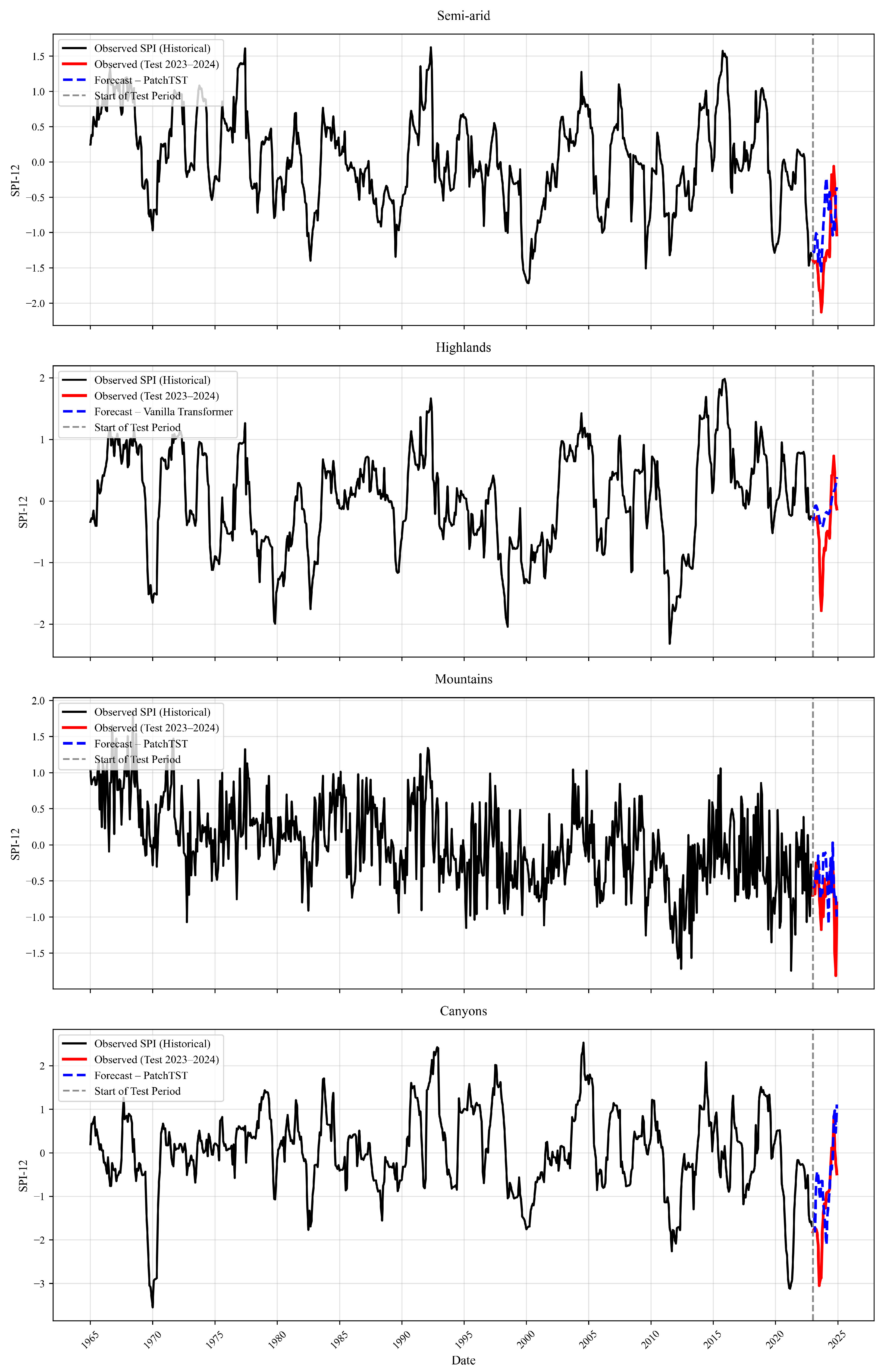
Figure 5 illustrates the complete SPI time series for the four regions of Zacatecas (1965–2024), distinguishing training/validation (black), observed test values (red), and forecasts from the best-performing model per region (blue dashed). The forecasts closely follow the observed test data (2023–2024), demonstrating reasonable alignment with historical variability. In Semi-arid, Mountains, and Canyons, PatchTST captures both seasonal patterns and extreme drought events (SPI < −2) effectively. In Highlands, Vanilla Transformer accurately reproduces the less variable dynamics of this region, with minimal deviation in the test period.

Figure 6 illustrates the distribution of residuals for each Transformer model across the four regions. In general, residuals are centered around zero, confirming unbiased predictions in most cases. Negative median residuals indicate a systematic tendency to underpredict across most models and regions. However, noticeable differences in spread exist: the Highlands region shows the tightest interquartile range (indicating lower variability in errors), particularly for Vanilla Transformer and TFT, while the Canyons and Mountains exhibit wider distributions, reflecting greater challenge in modeling more variable SPI series. Outliers are present in all regions, especially for models with higher RMSE (e.g., Autoformer), but they remain within reasonable bounds for SPI values.

4. Discussion

This study demonstrates that Transformer-based architectures, particularly PatchTST, provide a substantial improvement for long-horizon (24-month) forecasting of the Standardized Precipitation Index (SPI-12) in semi-arid environments. PatchTST achieved the best overall performance in three of the four climatic regions of Zacatecas and showed statistically significant superiority over most competing models according to the Diebold–Mariano test.

The superior performance of PatchTST in the more variable Semi-arid, Mountains, and Canyons regions is largely attributable to its patch-based design, which effectively captures local seasonal structures while modeling global dependencies. In contrast, the Vanilla Transformer performed best in the less variable Highlands, suggesting that model complexity should be aligned with the intrinsic variability of the target series. Negative Pearson correlations observed in some models during the 2023–2024 test period likely reflect a phase-shift issue associated with the strong post-El Niño climatic transition, rather than outright predictive failure.

Several limitations should be noted regarding the current experimental design. The models implemented in this study are univariate, which limits the direct incorporation of large-scale climatological drivers such as the El Niño-Southern Oscillation (ENSO). Furthermore, the empirical evaluation relied on a single 24-month independent test period (2023–2024). This specific window coincided with an intense macro-climatic transition from a strong El Niño event to neutral and La Niña states. While this temporal boundary effectively subjects the networks to stress conditions, covering only one anomalous climate cycle constrains the ability to draw definitive conclusions about structural long-term generalization. To mitigate this test-period selection bias and enhance validation stability, future studies should prioritize the integration of a rolling-origin validation framework across extended multi-decadal horizons. Additionally, this research produced exclusively point forecasts, and classical statistical benchmarks (such as SARIMA) were not included, which represent clear opportunities for future methodological expansions.

Future research should address these limitations by incorporating multivariate inputs (e.g., ENSO indices), adopting rolling-origin cross-validation, and extending the analysis to probabilistic forecasts using quantile outputs or ensemble strategies, evaluated with proper scoring rules such as Continuous Ranked Probability Score.

From an operational perspective, the strong performance of PatchTST, especially in highly variable regions, represents a valuable advancement for strengthening drought early warning systems such as the Mexico Drought Monitor operated by CONAGUA. Overall, this study highlights the potential of Transformer models—particularly PatchTST—for improving long-horizon SPI forecasting in water-scarce semi-arid environments.

5. Conclusions

This study demonstrates that Transformer-based models, particularly PatchTST, offer a robust solution for long-horizon (24-month) SPI-12 forecasting in semi-arid environments. PatchTST achieved the best performance in three of the four climatic regions of Zacatecas and showed statistically significant superiority over most competing models according to the Diebold–Mariano test. The results also confirm that model suitability is region-dependent: PatchTST excelled in highly variable areas, while the Vanilla Transformer performed best in the more stable Highlands.

Key limitations include the univariate nature of the models and the relatively short out-of-sample test period coinciding with an ENSO phase transition. Future research should incorporate multivariate inputs (e.g., ENSO indices), rolling-origin validation, and probabilistic forecasting outputs.

Overall, the findings highlight the potential of Transformer architectures—especially PatchTST—to strengthen operational drought early warning systems such as the Mexico Drought Monitor (CONAGUA), supporting more timely and region-specific decision-making in water-scarce environments.

References

- Fares, A.; Awal, R.; Fares, S.; Johnson, A.; Valenzuela, H. Irrigation Water Requirements for Seed Corn and Coffee under Potential Climate Change Scenarios. J. Water Clim. Change 2016, 7, 39–51. [Google Scholar] [CrossRef] [Scilit]
- Nieto Ferreira, R.; Nissenbaum, M.; Rickenbach, T. Climate Change Effects on Summertime Precipitation Organization in the Southeast United States. Atmos. Res. 2018, 214, 348–363. [Google Scholar] [CrossRef] [Scilit]
- Hayes, M.; Svoboda, M.; Wall, N.; Widhalm, M. The Lincoln Declaration on Drought Indices: Universal Meteorological Drought Index Recommended. Bull. Am. Meteorol. Soc. 2011, 92, 485–488. [Google Scholar] [CrossRef] [Scilit]
- Koudahe, K.; Kayode, A.; Samson, A.; Adebola, A.; Djaman, K. Trend Analysis in Standardized Precipitation Index and Standardized Anomaly Index in the Context of Climate Change in Southern Togo. Atmos. Clim. Sci. 2017, 7, 401–423. [Google Scholar] [CrossRef]
- McKee, T.; Doesken, N.; Kleist, J. The Relationship of Drought Frequency and Duration to Time Scales. In Proceedings of the 8th Conference on Applied Climatology, Anaheim, CA, USA, 17–22 January 1993; Volume 17, pp. 179–183. [Google Scholar]
- Caloiero, T. Drought Analysis in New Zealand Using the Standardized Precipitation Index. Environ. Earth Sci. 2017, 76, 569. [Google Scholar] [CrossRef] [Scilit]
- Giddings, L.; Soto, M.; Rutherford, B.; Maarouf, A. Standardized Precipitation Index Zones for México. Atmósfera 2005, 18, 33–56. [Google Scholar]
- Taiwo, A.; Folorunso, S.; Ogunwobi, Z. Forecast Performance of Univariate Time Series and Artificial Neural Network Models. LAUJET J. Eng. Technol. 2019, 12, 67–71. [Google Scholar]
- Zhou, H.; Zhang, S.; Peng, J.; Zhang, S.; Li, J.; Xiong, H.; Zhang, W. Informer: Beyond Efficient Transformer for Long Sequence Time-Series Forecasting. Proc. AAAI Conf. Artif. Intell. 2021, 35, 11106–11115. [Google Scholar] [CrossRef] [Scilit]
- Magallanes-Quintanar, R.; Galván-Tejada, C.; Galvan-Tejada, J.; de Jesús Méndez-Gallegos, S.; Blanco-Macías, F.; Valdez-Cepeda, R. Artificial Neural Network Models for Prediction of Standardized Precipitation Index in Central Mexico. Agrociencia 2023, 57, 245–262. [Google Scholar] [CrossRef] [Scilit]
- Magallanes-Quintanar, R.; Galván-Tejada, C.; Galván-Tejada, J.; Méndez-Gallegos, S.d.J.; García-Domínguez, A.; Gamboa-Rosales, H. Narx Neural Networks Models for Prediction of Standardized Precipitation Index in Central Mexico. Atmosphere 2022, 13, 1254. [Google Scholar] [CrossRef] [Scilit]
- Magallanes-Quintanar, R.; Galván-Tejada, C.; Galván-Tejada, J.; Gamboa-Rosales, H.; Méndez-Gallegos, S.; García-Domínguez, A. Neural Hierarchical Interpolation for Standardized Precipitation Index Forecasting. Atmosphere 2024, 15, 912. [Google Scholar] [CrossRef] [Scilit]
- Magallanes-Quintanar, R.; Galván-Tejada, C.; Galván-Tejada, J.; Gamboa-Rosales, H.; Méndez-Gallegos, S.; García-Domínguez, A. Auto-Machine-Learning Models for Standardized Precipitation Index Prediction in North–Central Mexico. Climate 2024, 12, 102. [Google Scholar] [CrossRef] [Scilit]
- Esquivel-Saenz, P.; Ortiz-Gómez, R.; Zavala, M.; Flowers-Cano, R. Artificial Neural Networks for Drought Forecasting in the Central Region of the State of Zacatecas, Mexico. Climate 2024, 12, 131. [Google Scholar] [CrossRef] [Scilit]
- Pita-Díaz, O.; Ortega-Gaucin, D. Analysis of Anomalies and Trends of Climate Change Indices in Zacatecas, Mexico. Climate 2020, 8, 55. [Google Scholar] [CrossRef] [Scilit]
- Nie, Y.; Nguyen, N.; Sinthong, P.; Kalagnanam, J. A Time Series Is Worth 64 Words: Long-Term Forecasting with Transformers. arXiv 2023, arXiv:2211.14730. [Google Scholar] [CrossRef] [Scilit]
- Wu, H.; Xu, J.; Wang, J.; Long, M. Autoformer: Decomposition Transformers with Auto-Correlation for Long-Term Series Forecasting. Adv. Neural Inf. Process. Syst. 2021, 34, 22419–22430. [Google Scholar]
- Lim, B.; Arık, S.; Loeff, N.; Pfister, T. Temporal Fusion Transformers for Interpretable Multi-Horizon Time Series Forecasting. Int. J. Forecast. 2021, 37, 1748–1764. [Google Scholar] [CrossRef] [Scilit]
- Alsharef, A.; Aggarwal, K.; Kumar, M.; Mishra, A. Review of ML and AutoML Solutions to Forecast Time-Series Data. Arch. Comput. Methods Eng. 2022, 29, 5297–5311. [Google Scholar] [CrossRef] [Scilit]
- Waqas, M.; Humphries, U. A Critical Review of RNN and LSTM Variants in Hydrological Time Series Predictions. MethodsX 2024, 13, 102946. [Google Scholar] [CrossRef] [Scilit] [PubMed]
- Pathania, A.; Gupta, V. Interpretable Transformer Model for National Scale Drought Forecasting: Attention-Driven Insights across India. Environ. Model. Softw. 2025, 187, 106394. [Google Scholar] [CrossRef] [Scilit]
- Shang, J.; Zhao, B.; Hua, H.; Wei, J.; Qin, G.; Chen, G. Application of Informer Model Based on SPEI for Drought Forecasting. Atmosphere 2023, 14, 951. [Google Scholar] [CrossRef] [Scilit]
- R Core Team. R: A Language and Environment for Statistical Computing; R Foundation for Statistical Computing: Vienna, Austria, 2024. [Google Scholar]
- Beguería, S.; Vicente-Serrano, S. SPEI: Calculation of the Standardised Precipitation-Evapotranspiration Index, R Package Version 1.8.1. 2017. Available online: https://climatedataguide.ucar.edu/climate-data/standardized-precipitation-evapotranspiration-index-spei (accessed on 1 March 2026).
- Farajzadeh, J.; Fakheri Fard, A.; Lotfi, S. Modeling of Monthly Rainfall and Runoff of Urmia Lake Basin Using “Feed-Forward Neural Network” and “Time Series Analysis” Model. Water Resour. Ind. 2014, 7–8, 38–48. [Google Scholar] [CrossRef] [Scilit]
- Lara-Benítez, P.; Carranza-García, M.; Riquelme, J. An Experimental Review on Deep Learning Architectures for Time Series Forecasting. arXiv 2021, arXiv:2103.12057. [Google Scholar] [CrossRef] [Scilit] [PubMed]
- Olivares, C.; Challú, C.; Garza, F.; Canseco, M.; Dubrawski, A. NeuralForecast: User-Friendly State-of-the-Art Neural Forecasting Models, R package version 1.0.0; Nixtlaverse: San Francisco, CA, USA, 2022.
- Vaswani, A.; Shazeer, N.; Parmar, N.; Uszkoreit, J.; Jones, L.; Gomez, A.N.; Kaiser, Ł.; Polosukhin, I. Attention Is All You Need. In Advances in Neural Information Processing Systems; Guyon, I., Luxburg, U.V., Bengio, S., Wallach, H., Fergus, R., Vishwanathan, S., Eds.; Curran Associates, Inc.: Red Hook, NY, USA, 2017; Volume 30, pp. 5998–6008. [Google Scholar]