Highlights
What are the main findings?
- A simple price threshold of 0.80 is introduced as a novel and robust real-time indicator for stablecoin failure, validated against benchmarks like CoinMarketCap delistings and volume-based methods.
- Lagged monthly market capitalization and stablecoin volatility are identified as the most significant predictors of default. These coin-specific drivers consistently outperform macroeconomic factors, and the panel Cauchit model with fixed effects (Cauchit FE) delivers the best out-of-sample forecasting performance.
What is the implication of the main findings?
- Investors and risk managers gain a practical, interpretable framework to assess stability. The 0.80 threshold can be used as a real-time signal to reassess risk or exit positions, while low volatility and high market capitalization serve as key indicators of a stablecoin’s resilience.
- Regulators can use the proposed threshold and forecasting models to monitor stablecoin stability and potential systemic risks in the DeFi market. The findings also imply that oversight should prioritize stablecoin-specific factors like reserve quality and transparency over broader macroeconomic controls.
Abstract
In this study, we extend research on stablecoin credit risk by introducing a novel rule-of-thumb approach to determine whether a stablecoin is “dead” or “alive” based on a simple price threshold. Using a comprehensive dataset of 98 stablecoins, we classify a coin as failed if its price falls below a predefined threshold (e.g., $0.80), validated through sensitivity analysis against established benchmarks such as CoinMarketCap delistings and Feder et al. (2018) methodology. We employ a wide range of panel binary models to forecast stablecoins’ probabilities of default (PDs), incorporating stablecoin-specific regressors. Our findings indicate that panel Cauchit models with fixed effects outperform other models across different definitions of stablecoin failure, while lagged average monthly market capitalization and lagged stablecoin volatility emerge as the most significant predictors—outweighing macroeconomic and policy-related variables. Random forest models complement our analysis, confirming the robustness of these key drivers. This approach not only enhances the predictive accuracy of stablecoin PDs but also provides a practical, interpretable framework for regulators and investors to assess stablecoin stability based on credit risk dynamics.
Keywords:
stablecoins; crypto-assets; cryptocurrencies; credit risk; probability of default; probability of death; panel binary models; fixed effects; cauchit; ZPP JEL Classification:
C32; C35; C51; C53; C58; G12; G17; G32; G33
1. Introduction
Stablecoins, designed to maintain a stable value typically pegged to $1, have emerged as critical components of decentralized finance (DeFi), powering transactions, lending, and liquidity provision in digital asset markets. With billions of dollars locked in DeFi protocols, stablecoins facilitate seamless interactions across blockchain ecosystems. However, their promise of stability has been repeatedly tested by high-profile failures. The collapse of TerraUSD in 2022, where the price fell precipitously below the $0.80 threshold we validate in this study, exposed catastrophic credit risks and triggered widespread market disruptions. These events underscore the urgent need for robust, real-time tools to assess and predict stablecoin stability—a need echoed by regulators like the Financial Stability Oversight Council [1] concerned about systemic risks. These events underscore the urgent need for robust tools to assess and predict stablecoin stability, both to protect investors and to address regulatory concerns about systemic risks in digital markets [2].
Despite their importance, the literature on stablecoin risk assessment remains limited in offering practical, real-time solutions. Prior studies, such as [3], focus on peg maintenance mechanisms, highlighting the role of reserves and arbitrage in ensuring stability. Others, like [2], warn of systemic risks from algorithmic stablecoins prone to runs, while [4] emphasize liquidity and regulatory challenges. However, these works often overlook simple, interpretable methods for detecting failures early. For instance, volume-based criteria, such as those adapted from [5] for cryptocurrencies, rely on lagging indicators like trading volume drops, which fail to capture depegging events in real time. Moreover, existing models rarely prioritize coin-specific predictors, such as market capitalization and volatility, which drive stablecoin survival compared to macroeconomic factors; see [6].
This study addresses these gaps by proposing a straightforward, data-driven framework to detect stablecoin failures and forecast probabilities of default (PDs). First, we introduce a novel rule-of-thumb: a stablecoin is classified as “dead” if its price falls below $0.80, a threshold validated against CoinMarketCap delistings and volume-based benchmarks. This approach enables real-time monitoring, overcoming the delays of traditional indicators. Second, we develop a large suite of panel binary models, including Cauchit fixed-effects (FE) and random-effects (RE) models, to forecast PDs, with lagged monthly market capitalization and stablecoin volatility as primary predictors. These models achieve superior out-of-sample performance, with AUC up to 0.947 and H-measure up to 0.842 for 30-day forecasts. Third, we validate the framework’s robustness using a time series-based Zero Price Probability (ZPP) model to forecast PDs, as well as different categorizations of stablecoins into long-lived and short-lived groups, depending on the length of their time series.
Beyond traditional binary response models, recent research in financial econometrics has increasingly emphasized frameworks that represent market conditions or asset states through latent binary or multi-state processes evolving over time. In particular, hidden Markov models (HMMs), Markov-switching regressions, and other state-space approaches have been employed to capture discrete shifts between stable and turbulent regimes in returns, volatility, or liquidity [7,8,9]. Similar probabilistic state representations have also been applied to the cryptocurrency market to identify regime transitions associated with crashes or depegging episodes [10,11]. These models share a conceptual link with the threshold-based binary framework adopted in this paper: in both cases, the system alternates between discrete states driven by past information. However, while regime-switching or state-space models infer transitions probabilistically, the present analysis relies on explicit and optimized threshold rules that directly map observable predictors (such as lagged market capitalization and volatility) into failure or survival states. Our threshold-based classification approach provides a transparent, real-time analog to these more complex state representations, offering practical advantages for regulatory monitoring and risk management applications.
The contributions of this study are threefold: it provides a simple, transparent $0.80 price threshold for immediate failure detection, a set of high-performing panel models for PD forecasting, and robustness checks that reinforce the importance of stablecoin market capitalization and volatility over external factors, aligning with S&P Global Ratings’ [12] emphasis on stablecoin reserve quality. These tools offer practical value for investors seeking to manage credit risk and regulators monitoring DeFi stability, addressing critical gaps in the literature. By focusing on coin-specific dynamics and real-time applicability, this study provides an actionable framework to navigate the complex and rapidly evolving stablecoin market.
2. Literature Review
Early studies on stablecoins focused on their design and stabilization mechanisms. Ref. [3] examined the factors maintaining stablecoin pegs, highlighting the role of reserve backing and market confidence in fiat-collateralized stablecoins like Tether (USDT) and USD Coin (USDC). They found that deviations from the peg are often temporary and corrected through arbitrage, though transparency in reserve management remains a persistent concern. In contrast, algorithmic stablecoins, which rely on smart contracts to adjust supply and demand, have been critiqued for their inherent fragility. Ref. [2] likened these to historical private currencies prone to runs—a view reinforced by the TerraUSD collapse, where a loss of investor confidence triggered a rapid depeg and systemic contagion within DeFi markets.
Building on this foundation, Ref. [6] marked a significant advancement by explicitly estimating the credit risk of stablecoins, in what was the first study to focus exclusively on this market segment. Using [5]’s methodology, they identified that 21% of a sample of 121 stablecoins were “abandoned” at least once, with only 36% achieving subsequent “resurrection” and 11% maintaining that status. They employed structural break tests to detect significant peg deviations, finding an average of 10 days between a break and a coin’s collapse or stabilization. Probabilities of default (PDs) were estimated using market-capitalization-based forecasting models, revealing that stablecoins on robust blockchains like Ethereum exhibited lower default risk. These findings underscored the importance of coin-specific factors—–such as market capitalization and blockchain ecosystem strength—in assessing credit risk, beyond the broader market dynamics explored in earlier works.
Prior financial literature has examined stablecoin credit risk, particularly in the context of regulatory and financial stability concerns. Ref. [4] analyzed stablecoins’ role within the crypto-asset ecosystem, noting their critical function as liquidity providers in DeFi and their potential to transmit risks to traditional financial systems. They highlighted operational, liquidity, and settlement risks, exacerbated by inadequate redemption policies among major issuers like Tether, which imposes weekly redemption limits or high minimum thresholds. This evidence aligns with recent observations of stablecoin vulnerabilities highlighted by [6] and motivates our proposal of a rule-of-thumb threshold to detect failure events.
More recently, the 2024 Annual Report by the U.S. Financial Stability Oversight Council (FSOC) [1], released in December 2024, warned that stablecoins remain a potential risk to financial stability, citing their vulnerability to runs in the absence of robust risk management standards. This report underscores ongoing policy attention to credit risk, complementing our empirical focus. Additionally, S&P Global Ratings [12] evaluated the creditworthiness of USDC, emphasizing reserve transparency and liquidity management as key stability drivers, though it stopped short of econometric modelling. These works reinforce the relevance of stablecoin-specific variables—such as market capitalization and volatility—over external factors, a hypothesis we test in this study.
Econometric approaches to stablecoin credit risk have also evolved. Ref. [6] employed the Zero-Price Probability (ZPP) model and the [13]’s Proportional Hazards model—a widely used framework in survival analysis—to forecast stablecoin PDs. Ref. [14] modeled the probability of death for over two thousand cryptocurrencies, including a small number of stablecoins, using credit scoring models, machine learning, and time-series-based methods, identifying market capitalization as a critical predictor. Interestingly, he also found that the (pooled) cauchit model and the ZPP model were the best approaches for newly established coins, whereas credit-scoring models and machine-learning methods were better suited for older coins. Given this evidence and our available dataset, we extend the cauchit model to a panel setting to capture potential unobserved heterogeneity.
The literature has also explored alternative predictors of stablecoin stability. Ref. [15] modeled multivariate market and credit risks for cryptocurrencies, finding volatility to be a significant driver—a result we confirm for stablecoins in this study. Conversely, macroeconomic variables such as policy indices or Bitcoin volatility, while influential in broader crypto markets [4], appear less critical for forecasting stablecoin PDs, a distinction we investigate further. Economic intuition suggests that short-term lags (e.g., daily) capture immediate market shocks affecting peg stability, while longer lags (e.g., monthly) reflect persistent trends in investor confidence and liquidity, as stablecoins are less volatile than other cryptocurrencies [3]. Moreover, Ref. [3] examined how improved arbitrage mechanisms stabilize stablecoin prices and consistently highlighted market capitalization and volatility as dominant features.
In summary, the stablecoin literature has evolved from design analyses to PD modeling, emphasizing coin-specific variables under regulatory scrutiny. Our study advances this with threshold-based detection and panel models.
3. Methodology
This section outlines the methodology employed to assess stablecoin credit risk and forecast their probabilities of default (PDs). It is structured into three subsections: detecting stablecoin failure using threshold rules, modelling PDs with panel binary and random forest models, and evaluating forecasting performance with specific metrics.
3.1. Detecting Stablecoin Failure with Simple Thresholds
We introduce a novel rule-of-thumb approach to classify stablecoins as dead or alive, based on a simple price threshold applied to their closing prices. A stablecoin is deemed dead (Status = 1) if its price falls below a predefined threshold (e.g., $0.80), and alive (Status = 0) otherwise.
Economically, a threshold like $0.80 reflects the point where depegging erodes investor confidence, triggering potential runs or liquidity crises, as stablecoins’ value proposition relies on near-$1 parity; we validate this via sensitivity analysis across $0.05 to $0.95 against benchmarks like CoinMarketCap delistings. To operationalize this, we define Status variables across a range of thresholds from $0.05 to $0.95 in increments of $0.05, using two panel datasets: stablecoins with fewer than 730 observations (11,558 observations across 39 coins) and stablecoins with more than 730 observations (76,176 observations across 59 coins). We compare our approach to existing benchmarks, such as the CoinMarketCap delisting criterion and the methodology proposed in [5], which we use to validate our threshold-based classification through a detailed sensitivity analysis.
CoinMarketCap, a leading cryptocurrency data aggregator, delists a crypto-asset when it no longer meets specific listing criteria, such as sufficient trading volume, liquidity, or project activity. See the detailed requirements here: (https://coinmarketcap.com/academy/glossary/delisting, accessed on 15 November 2025). Delisting typically occurs when a coin is deemed inactive or abandoned by its developers, often following a significant decline in market relevance or a failure to maintain its peg (in the case of stablecoins). In our sample of 98 stablecoins, 25 were delisted from CoinMarketCap by the end of the observation period, providing a benchmark for “dead” status. However, delisting is a lagging indicator, as it reflects decisions made after a coin’s decline and lacks transparency regarding exact thresholds, necessitating alternative methods for real-time detection.
The methodology in [5] offers another approach to identify crypto-asset failure. However, its original approach, which identifies failure based on price peaks, is unsuitable for stablecoins designed for price stability; see [6] and references therein. To address this, we adapt their method to focus solely on trading volume. In our modified approach, a “candidate peak” is defined as the date when the 7-day rolling average trading volume surpasses any recorded volume within a surrounding 30-day period, both forward and backward. Following a similar filtering process to the original method [5], we retain only those volume peaks that exceed the lowest observed volume in the preceding 30 days by at least 50% and account for at least 5% of the stablecoin’s all-time maximum trading volume. Once these volume-based peaks are identified, each is assessed against subsequent daily trading volumes, and we apply the final classification rules unchanged: a stablecoin is deemed “dead” if its average daily trading volume falls below 1% of its peak volume. Conversely, a previously “dead” stablecoin is reclassified as “resurrected” if its trading volume recovers to exceed 10% of its peak volume. This volume-centric adaptation provides a more effective measure of stablecoin abandonment.
An important caveat of the volume-based Feder criterion, and any methodology relying on reported trading volume in cryptocurrency markets, is the potential impact of wash trading and other forms of volume manipulation. Wash trading—the practice of simultaneously buying and selling an asset to create artificial activity—is a known issue on some cryptocurrency exchanges [16,17]. This manipulation can artificially inflate reported trading volumes, creating a misleading impression of liquidity and market interest. In the context of our adapted Feder method, sustained wash trading could potentially delay the classification of a stablecoin as “dead” by keeping its average daily trading volume artificially above the 1% of peak volume threshold, even if genuine economic activity and organic market demand have evaporated. This inherent vulnerability to data manipulation further motivates the need for alternative, more robust failure detection methods, such as our price-threshold approach, which is based on the more directly observable and economically fundamental metric of price stability.
In this study, we applied only the volume-based Feder et al. method [5] to our sample of 98 stablecoins, alongside our threshold-based approach, to compare their effectiveness. Table 1 presents these classifications for all 98 stablecoins, displaying the CoinMarketCap (final) listing status, the outcomes from the volume-based approach [5] (number of deaths, resurrections, and final status), and the results of our price threshold method at $0.80 (number of deaths, resurrections, and final status).

Table 1.
A stablecoin-by-stablecoin comparison of failure classification using three distinct methods. The table reports the final listing status from CoinMarketCap, alongside the number of failure (’death’) and recovery (’resurrection’) events detected by the volume-based Feder et al. (2018) method and our proposed $0.80 price threshold method. ’Final Status’ indicates whether the stablecoin was classified as ’Dead’ or ’Alive’ at the end of the sample period according to each dynamic method.
For validation, we performed a sensitivity analysis comparing our threshold-based method to the CoinMarketCap and Feder benchmarks. We considered two classification criteria: Final Status (a stablecoin is classified as dead if its price remains below the threshold at the end of the sample) and Dynamic Threshold (a stablecoin is classified as dead if its price drops below the threshold at least once during its lifetime). We computed overlap percentages for dead coins, alive coins, and overall accuracy (i.e., both dead and alive combined). Table 2 reports these results for thresholds ranging from $0.05 to $0.95, using CoinMarketCap (25 dead, 73 alive) and the Feder volume-only method (39 dead/59 alive for Final Status and 41 dead/57 alive for Dynamic Threshold) as reference classifications.
Table 2.
Sensitivity analysis of our price-based failure classification method. This table evaluates the classification overlap (in percentage) between various price thresholds (from $0.05 to $0.95) and two benchmarks: CoinMarketCap delistings and the volume-based Feder et al. (2018) method. The analysis is presented for two scenarios: ’Final Status’ assesses classification at the end of the sample, while ’Dynamic Threshold’ classifies a coin as dead if it ever breached the threshold. The $0.80 threshold, used in our main analysis, is highlighted in bold.
At a threshold of $0.80, our approach identifies 25 stablecoins as “dead” under the Final Status criterion, with an overlap of 52% with CoinMarketCap delistings and 41.03% with the method proposed by [5]. When applying the Dynamic Threshold criterion, our method identifies 32 dead stablecoins, increasing the overlap to 56% with CoinMarketCap and 53.66% with the Feder method. Raising the threshold to $0.85 increases the proportion of detected dead coins (60% and 72% overlap with CoinMarketCap for the Final and Dynamic criteria, respectively), but decreases the overlap for alive coins. This trade-off suggests that $0.80 serves as a balanced and practical threshold for detecting stablecoin failure.
This specific threshold is further supported by a straightforward price distribution analysis, where we examine histograms of both the final observed prices and the minimum prices of stablecoins over their respective time series. This visualization, presented in Figure 1, illustrates where most stablecoins’ prices lie relative to the $0.80 threshold, reinforcing its empirical relevance as a benchmark for classification.
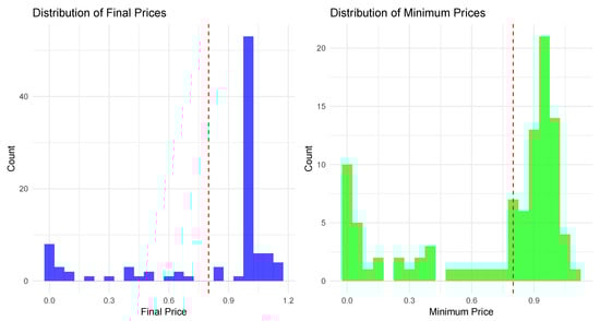
Figure 1.
Visual justification for the $0.80 failure threshold. The figure displays histograms for two key price points across the 98 stablecoins in our sample: their final observed price (left panel) and their all-time minimum price (right panel). The red vertical line at $0.80 illustrates how this threshold effectively separates the distribution of failed or distressed stablecoins (concentrated below the line) from those that maintained their peg (concentrated near $1.00).
At a conceptual level, the choice of a $0.80 threshold is rooted in established financial principles where a 20% deviation from a target price is widely recognized as a signal of a structural break or bear market. For a stablecoin, this threshold is not arbitrary: it represents a critical point where its primary function—to maintain its peg—has fundamentally failed. Economically, a persistent drop to $0.80 erodes the coin’s perceived ‘moneyness’ [3] and often triggers automated risk-management protocols, margin calls, and liquidation cascades, particularly in leveraged DeFi environments. It serves as a psychological coordination point where investors collectively reassess the asset’s credibility, potentially leading to a terminal loss of confidence, as exemplified by the TerraUSD collapse [18]. This threshold thus provides an economically meaningful and empirically observable boundary for classifying failure.
Therefore, by leveraging both sensitivity analysis and price distribution insights, our approach offers a real-time, transparent, and interpretable alternative to existing failure detection methods. Unlike CoinMarketCap’s delisting process, which operates with inherent delays, or the volume-based method in [5], which relies solely on trading activity, our price-based threshold provides an immediate and robust indicator of stablecoin distress. This novel approach enhances risk assessment by offering a clear, data-driven framework that can be easily implemented by researchers, investors, and regulators seeking timely insights into stablecoin stability.
3.2. Models for Stablecoin Probability of Default Forecasting
We briefly discuss the models employed to forecast the probability of default (PD) for stablecoins. Following [14,15,19], direct forecasts were computed using lagged regressors. Specifically, 1-day lagged regressors were used to forecast the 1-day ahead PD, 30-day lagged regressors for the 30-day ahead PD, and for stablecoins with over 730 observations, 365-day lagged regressors for the 365-day ahead PD. These specific forecast horizons were chosen to capture distinct economic risk dimensions: 1-day ahead for immediate market shocks and liquidity stress, 30-day ahead to align with medium-term portfolio and reporting cycles, and 365-day ahead to assess long-term viability, analogous to traditional annual credit risk. The regressors included lagged changes in market capitalization, stablecoin historical volatility, Bitcoin implied volatility, and economic policy uncertainty indexes (further details are provided in the Empirical section below).
The following models estimate the probability of default for stablecoin i at time t. The vector contains the lagged regressors for stablecoin i at time t.
- Pooled Logit Model: The pooled logit model assumes homogeneity across stablecoins, ignoring the panel structure. The probability of default is modeled as:where is the binary outcome (1 for default, 0 otherwise), is the vector of regressors, and is the vector of coefficients.
- Panel Logit Model with Fixed Effects: This model accounts for unobserved heterogeneity across stablecoins by including individual-specific intercepts :
- Panel Logit Model with Fixed Effects and Asymptotic Bias Correction: Fixed effects logit models suffer from the incidental parameters problem, leading to biased estimates in short panels. To mitigate this, asymptotic bias correction methods based on [20], and [21,22] were applied. These methods adjust the estimated coefficients to reduce bias:where is the fixed effects estimator. See also [23] for more details.
- Conditional Logit Model: This model eliminates the individual fixed effects by conditioning on the sum of for each stablecoin. The probability is given by:The denominator sums over all time observations for each stablecoin, representing the conditional probability given exactly one default of the stablecoin occurs.
- Panel Logit Model with Random Effects: The random effects model treats individual-specific effects as random variables drawn from a distribution, typically normal:where .
- Pooled Cauchit Model: The pooled cauchit model uses the Cauchy cumulative distribution function instead of the logistic function:
- Panel Cauchit Model with Fixed Effects: This model extends the pooled cauchit model by incorporating individual-specific intercepts:
- Panel Cauchit Model with Random Effects: This model introduces random effects into the cauchit framework:
- Random Forests Model: In addition to the panel binary models, a random forests model was employed. This non-parametric ensemble method builds multiple decision trees on random subsets of the data and averages their predictions. It was selected due to its proven effectiveness in forecasting PDs of cryptocurrencies, crypto exchanges, and in detecting pump-and-dump schemes involving crypto assets, as documented in [14,24,25].
The model was implemented using the randomForest package in R. We set the number of trees to to ensure stable predictions. All other hyperparameters were set to the package’s default values, which are standard in the literature and yielded robust performance. The key defaults include: the number of variables randomly sampled as candidates at each split (‘mtry’) was set to , where p is the total number of predictors; the minimum size of terminal nodes (‘nodesize’) was 1; and no maximum depth was enforced for the trees (‘maxnodes = NULL’). The Gini impurity index was used as the splitting criterion. Preliminary tuning indicated that the model’s performance was robust to variations in these parameters; therefore, we proceeded with these standard and well-established settings.
The predicted PD is given by:
where is the b-th tree in the ensemble.
We remark that the inclusion of the Cauchit model is motivated not only by its empirical performance but also by its theoretical suitability for the dynamics observed in cryptocurrency markets. The Cauchit specification, which employs the cumulative distribution function of the Cauchy distribution as its link function, features much heavier tails than the Logit or Probit alternatives. This heavy-tailed structure makes it more robust to outliers and extreme realizations, features that are pervasive in cryptocurrency data due to abrupt price jumps, liquidity shocks, and irregular trading activity. In such environments, the Cauchit link can better accommodate extreme values of the latent variable without allowing them to disproportionately influence coefficient estimates or predicted probabilities, thereby improving robustness and interpretability [26,27]. From a conceptual perspective, the Cauchit model is particularly well suited for modelling binary outcomes characterized by long periods of stability followed by sudden regime shifts, such as stablecoin defaults. For most of their lifespan, stablecoins exhibit near-zero probabilities of failure that remain largely insensitive to small fluctuations in volatility or market capitalization. However, when confidence erodes, due to events like a breakdown in arbitrage mechanisms or a run on reserves, the same explanatory variables can trigger a rapid, nonlinear jump in the probability of default. The fatter tails of the Cauchit link function capture this abrupt transition more effectively than the smoother response of the Logit model, allowing for a more realistic representation of these threshold-driven dynamics [28]. Moreover, the Cauchit model’s slower tail decay allows for flexible modelling of rare but economically meaningful events, where the probability mass in the extremes carries critical information about systemic fragility. This property makes it especially appropriate for stablecoin markets, where extreme depegging episodes (such as the TerraUSD collapse) represent defining moments for the system’s stability. Its robustness to heavy-tailed distributions ensures more stable parameter estimates even in the presence of volatile price movements or sudden market capitalization changes. Additionally, when applied to panel data, the Cauchit specification accommodates unobserved heterogeneity across stablecoins with varying lifespans, further enhancing its suitability for this context. These theoretical advantages, together with its strong empirical performance with cryptoassets [14], justify its inclusion alongside the Logit and Probit models as a robustness check against thin-tailed assumptions.
3.3. Evaluation Metrics for Binary Models
To assess the predictive performance of our models in forecasting stablecoin probabilities of default (PDs), we employ several standard evaluation metrics for binary classification: the Area Under the receiver operating characteristic Curve (ROC AUC), the H-measure by [29], the Brier score [30], and classification accuracy, sensitivity, and specificity under different thresholding approaches.
- ROC AUC
The receiver operating characteristic (ROC) curve plots the true positive rate (TPR) against the false positive rate (FPR) at varying classification thresholds. The true positive rate, also known as sensitivity or recall, is given by:
where TP (true positives) represents correctly classified positive cases, and FN (false negatives) denotes misclassified positive cases. The false positive rate is defined as:
where FP (false positives) represents misclassified negative cases, and TN (true negatives) denotes correctly classified negative cases. The area under the ROC curve (AUC) summarizes the overall performance, with a value of 0.5 indicating random guessing and 1 representing perfect classification; see [31] for more details.
- H-measure
The H-measure, introduced by [29], addresses key limitations of the ROC AUC metric by explicitly incorporating application-specific misclassification costs. While AUC evaluates a classifier’s ability to rank positive instances above negative ones across all possible thresholds, it does not account for situations where ROC curves intersect or where certain regions of the curve are more relevant—such as minimizing false positives in financial risk assessment. The H-measure overcomes these limitations by defining an optimal classification threshold that minimizes the expected misclassification cost, given by:
where represents the severity ratio, which adjusts the relative misclassification costs for the two classes , while denotes the class priors and the cumulative distribution function of predicted scores for class i. The misclassification loss at a threshold t is then:
The general loss is obtained by substituting the optimal threshold from (12) into (13). This value is then weighted using a Beta severity distribution and integrated over all possible severity ratios c [32]:
where the Beta distribution parameters are defined as and .
The H-measure is then defined as the normalized ratio of the general loss to the worst-case loss scenario:
This formulation allows the H-measure to adapt to real-world cost structures, making it particularly useful in domains such as fraud detection and credit risk modelling, where false positives and false negatives carry asymmetric consequences.
- Brier Score
The Brier score quantifies the accuracy of probabilistic predictions by computing the mean squared error between the predicted probability and the true binary outcome :
where N is the total number of observations. Lower Brier scores indicate better calibration of the model’s probability estimates.
- Accuracy, Sensitivity, and Specificity
Classification performance is also assessed using accuracy, sensitivity, and specificity, computed under two thresholding schemes: (i) a fixed threshold of 50% and (ii) the empirical prevalence of positive cases in the dataset. Accuracy measures overall correctness and is given by:
Sensitivity (or recall) is computed using Equation (10), while specificity, which measures the proportion of correctly identified negative cases, is defined as:
By evaluating these metrics across different thresholds, we ensure a comprehensive assessment of model discrimination, calibration, and classification performance.
- The Model Confidence Set (MCS) Procedure
The Model Confidence Set (MCS), introduced by [33], is a statistical framework designed to compare forecasting models while accounting for uncertainty. Unlike conventional selection methods that pinpoint a single best model, the MCS approach identifies a subset of models that are statistically equivalent to the best-performing model at a given confidence level. This procedure employs an iterative hypothesis testing process to systematically remove underperforming models. It begins with an initial set of candidate models, denoted as , consisting of models. The performance of each model is assessed using a predefined loss function. In the case of binary classification, a commonly used loss function is the Brier score (16).
The objective of the MCS procedure is to retain a subset of models, denoted as , that are not significantly worse than the best-performing model in . This is achieved by testing the null hypothesis that the expected loss difference between all model pairs is zero:
where represents the difference in loss between models i and j. To assess the relative performance of models, test statistics based on the loss differences are computed. Two commonly used statistics are the Range Statistic:
where denotes the sample mean of , and the T-Statistic:
where represents the average loss difference of model i relative to all other models.
Through an iterative elimination process, models that fail the hypothesis test are progressively excluded until the remaining models form a set in which performance differences are no longer statistically significant at a given confidence level . By applying the MCS procedure, we identify a robust subset of models that deliver comparably strong performance in probabilistic forecasting of binary outcomes. This approach is particularly valuable in financial applications, where ensuring model reliability and interpretability is essential, and minor predictive improvements can lead to meaningful practical outcomes.
4. Empirical Analysis
4.1. Data
We collected daily data on 98 stablecoins from three primary cryptocurrency data platforms: CoinMarketCap, CoinGecko, and TokenInsight. CoinMarketCap (https://coinmarketcap.com, accessed on 15 November 2025) is a widely recognized aggregator that provides historical and real-time data on cryptocurrency prices, market capitalization, and trading volumes, alongside listing status updates. CoinGecko (https://www.coingecko.com, accessed on 15 November 2025) offers a complementary dataset, tracking similar metrics with an emphasis on community-driven insights and additional market indicators. TokenInsight (https://tokeninsight.com, accessed on 15 November 2025) provides detailed analytics on blockchain assets, including stablecoins, with a focus on risk ratings and market performance. Given that data for some stablecoins are no longer available online due to delisting or project abandonment, we supplemented our dataset using the Wayback Machine (https://web.archive.org/,waybackmachine, accessed on 15 November 2025) [34]. The Wayback Machine is an initiative by the Internet Archive that archives snapshots of websites over time, enabling us to retrieve historical data from these platforms when primary sources were inaccessible. The full list of stablecoins analyzed is reported in Table 1 of Section 3.1 (“Detecting Stablecoin Failure with Simple Thresholds”).
Our dataset includes daily observations of open, high, low, and close prices, market capitalization, and trading volume for these 98 stablecoins, spanning January 2019 to November 2024. Following [14], we categorized the coins into two groups based on observation count: 39 stablecoins with fewer than 730 observations, used to forecast 1-day and 30-day ahead probabilities of death, and 59 stablecoins with more than 730 observations, used to forecast 1-day, 30-day, and 365-day ahead probabilities of death. For each stablecoin, we computed several market capitalization differences: today’s value minus yesterday’s (), today’s minus 7 days ago (), and today’s minus 30 days ago (). Additionally, we calculated daily stablecoin volatility using a modified estimator [35] that accounts for opening gaps, as proposed by [36], and defined as:
where , , , and denote the open, high, low, and close prices on day t. We also computed weekly and monthly rolling averages of the daily historical volatilities. This regressor structure, incorporating daily, weekly, and monthly horizons, draws inspiration from the Heterogeneous Auto-Regressive (HAR) model in [37].
The selection of daily, weekly, and monthly horizons for market capitalization changes and volatility captures both immediate market reactions and sustained trends, providing a comprehensive view of stability dynamics across different time frames relevant to investors and regulators.
We included the T3 Bitcoin Volatility Index [38], a 30-day implied volatility (IV) measure for Bitcoin derived from Bitcoin option prices via linear interpolation between the expected variances of the two nearest expiration dates. Sourced from (https://t3index.com/indexes/bit-vol/, accessed on 15 January 2025) until its discontinuation in February 2025, the full methodology is archived at (https://web.archive.org/web/20221114185507/https://t3index.com/wp-content/uploads/2022/06/Bit-Vol-process_guide-Jan-2019-2022_03_22-06_02_32-UTC.pdf, accessed on 15 November 2025). We also computed weekly and monthly rolling averages of this index for each stablecoin. Alternative implied volatility indices exist, such as those from Deribit (https://www.deribit.com, accessed on 15 November 2025), a leading crypto options exchange that calculates volatility from its Bitcoin and Ethereum option markets, and other institutions like Skew or CryptoCompare, which provide similar metrics. The Bitcoin IV is potentially an important regressor because Bitcoin volatility often drives broader crypto market dynamics, potentially destabilizing stablecoins through correlated price shocks or shifts in investor confidence, thereby influencing their probability of default.
The daily news-based Economic Policy Uncertainty (EPU) Index, sourced from (https://www.policyuncertainty.com/us_monthly.html, accessed on 15 November 2025), is constructed from newspaper archives in the NewsBank Access World News database, which aggregates thousands of global news sources. We restricted our analysis to newspaper articles, excluding magazines and newswires, to ensure consistency. Weekly and monthly rolling averages of this index were also computed for each stablecoin. The EPU Index captures macroeconomic and policy-related uncertainty, which may affect stablecoin stability by altering investor risk appetite or triggering capital flows that impact peg maintenance, making it a relevant predictor of PDs. This index has been successfully used in a large number of academic and professional articles; see (https://www.policyuncertainty.com/research.html, accessed on 15 November 2025) and all references therein. A notation Table A14 was added in the Appendix A that lists all our main variables.
Differently from past literature (see [14] and references therein), we excluded daily Google Trends data on stablecoin searches due to several limitations: for many stablecoins, daily data were unavailable because search volumes fell below Google Trends’ reporting threshold, which standardizes searches between 0 and 1 only for sufficient activity. Moreover, for coins with available data, searches predominantly reflected interest in the real dollar rather than the stablecoin, introducing noise and potential bias. Thus, we discarded this variable entirely. Furthermore, we did not consider Google Trends data for Bitcoin in our analysis, following the evidence provided by [39,40]. These studies compared the predictive performance of models using implied volatility against those using Google search data for forecasting volatility and risk measures across various financial and commodity markets. Their findings indicate that implied volatility models generally outperform those based on Google Trends data. This result is attributed to the fact that the information captured by Google search activity is already embedded within implied volatility, whereas the reverse does not hold. These authors argue that this is likely because implied volatility reflects the forward-looking expectations of sophisticated market participants—such as institutional investors with access to superior information—while Google Trends primarily reflect the behavior and expectations of retail investors with limited information.
As detailed in Section 3.1, we applied two competing criteria to classify stablecoins daily as dead or alive/resurrected: the volume-based approach in [5], and our price threshold method at $0.80, deeming a coin dead if its price falls below 80 cents, and alive or resurrected if above or recovering above 80 cents, respectively. The CoinMarketCap final listing status was not used for daily analysis, as it reflects only the end-of-sample status. The dataset of 39 stablecoins with fewer than 730 observations spans February 2021 to November 2024 (11,558 daily observations), while the 59 stablecoins with more than 730 observations span January 2019 to November 2024 (76,176 daily observations). Following [14,15], we employed direct forecasts, using 1-day lagged regressors for 1-day ahead PDs, 30-day lagged regressors for 30-day ahead PDs, and, for coins with over 730 observations, 365-day lagged regressors for 365-day ahead PDs.
Table 3 reports the total number of “dead days”—days when stablecoins are classified as dead under the two criteria—both in absolute value and as a percentage.
Table 3.
Total count and percentage of “dead days” under two different failure classification criteria. The table shows the total number of days stablecoins were classified as failed, both for the volume-based Feder et al. (2018) method and our $0.80 price threshold method. Results are shown separately for stablecoins with shorter (<730 days) and longer (≥730 days) time series.
It appears that the price threshold method is more restrictive, requiring a significant price drop below 80 cents, whereas the volume-based Feder method captures more days as dead, potentially including periods of low activity that do not necessarily reflect a loss of peg stability.
Figure 2 illustrates the total number of stablecoins available each day (blue line) and the number of dead stablecoins each day according to the Feder method (green line) and the $0.80 threshold (red line), split by observation groups.
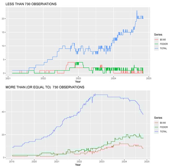
Figure 2.
Evolution of stablecoin failures over time according to two classification methods. The panels show results for stablecoins with fewer than 730 observations (top) and 730 or more (bottom). The blue line tracks the total number of active stablecoins each day. The green line represents the count of ’dead’ stablecoins using the volume-based Feder et al. (2018) method, while the red line shows the count using our $0.80 price threshold.
For stablecoins with fewer than 730 observations, the $0.80 method reacts more quickly to failure events, as seen in sharper spikes (e.g., August 2022 and mid-2023), while the Feder method shows more sustained periods of dead stablecoins, reflecting its sensitivity to prolonged low volume. For stablecoins with 730 or more observations, the $0.80 method again responds faster, with notable peaks (e.g., 2022), compared to the Feder method’s broader plateaus. This quicker reaction aligns with the price threshold’s focus on immediate peg deviations, making it a more responsive indicator of stablecoin distress in real-time monitoring scenarios.
4.2. In-Sample Analysis
The in-sample analysis evaluates the performance of various panel models and a random forest model in explaining the probability of stablecoin failure, using the full available data sample and the two classification criteria outlined in Section 3.1: the $0.80 price threshold and the volume-based approach of [5].
The in-sample results are visualized in Figure 3, Figure 4, Figure 5, Figure 6, Figure 7 and Figure 8. Specifically, Figure 3 and Figure 4 show the panel model coefficient estimates for the $0.80 price threshold approach, segmented by stablecoin lifespan (≥730 and <730 observations). The corresponding Random Forest variable importance measures are displayed in Figure 5. Similar visual summaries for the Volume-based Feder et al. (2018) approach are provided in Figure 6, Figure 7 and Figure 8. In the variable importance charts, results are broken down by lifespan and metric, with variables ranked and forecast horizons distinguished by color.
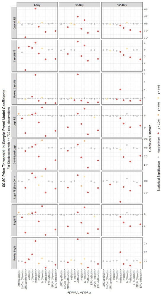
Figure 3.
In-sample coefficient estimates from various panel binary models for stablecoins with ≥730 observations, using the $0.80 price threshold for failure classification. Each panel corresponds to a different forecast horizon (1-day, 30-day, 365-day). The x-axis lists the predictor variables, and the y-axis shows the coefficients’ magnitudes and their statistical significance.
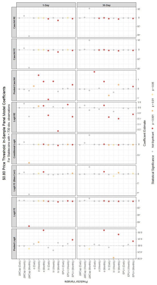
Figure 4.
In-sample coefficient estimates from various panel binary models for stablecoins with <730 observations, using the $0.80 price threshold for failure classification. Each panel corresponds to a different forecast horizon (1-day, 30-day, 365-day). The x-axis lists the predictor variables, and the y-axis shows the coefficients’ magnitudes and their statistical significance.
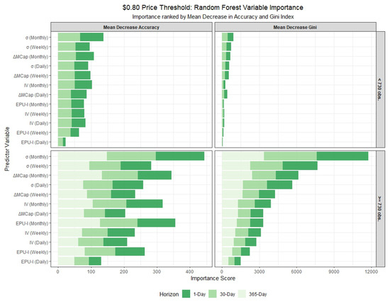
Figure 5.
In-sample variable importance from the Random Forest model, using the $0.80 price threshold definition of failure. The plots show results for stablecoins with fewer (<730) and more (≥730) observations across different forecast horizons. Importance is measured by Mean Decrease in Accuracy (MDA, higher is better) and Mean Decrease in Gini (MDG, higher is better). Variables are ranked by MDA, highlighting the most predictive features for each group and horizon.
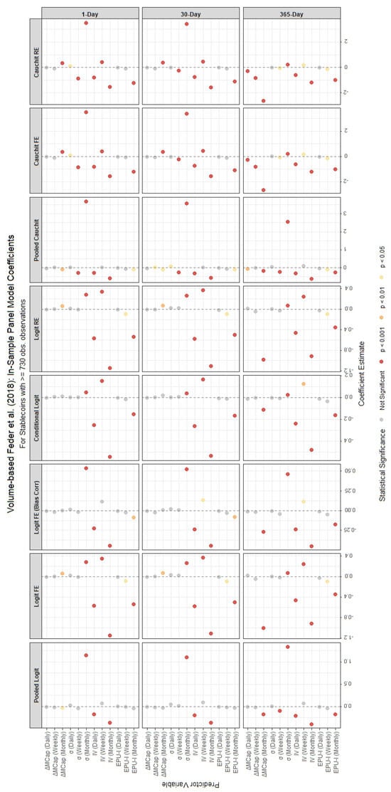
Figure 6.
In-sample coefficient estimates from various panel binary models for stablecoins with ≥730 observations, using the volume-based Feder et al. (2018) method for failure classification. Each panel corresponds to a different forecast horizon (1-day, 30-day, 365-day). The x-axis lists the predictor variables, and the y-axis shows the coefficients’ magnitudes and their statistical significance.
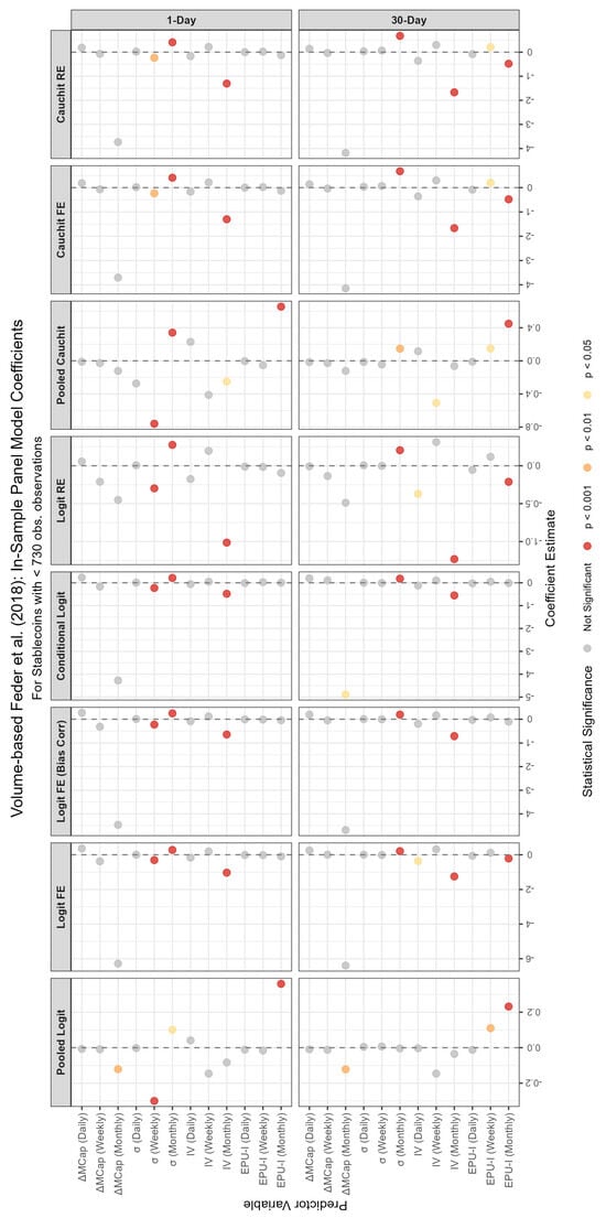
Figure 7.
In-sample coefficient estimates from various panel binary models for stablecoins with <730 observations, using the volume-based Feder et al. (2018) method for failure classification. Each panel corresponds to a different forecast horizon (1-day, 30-day, 365-day). The x-axis lists the predictor variables, and the y-axis shows the coefficients’ magnitudes and their statistical significance.
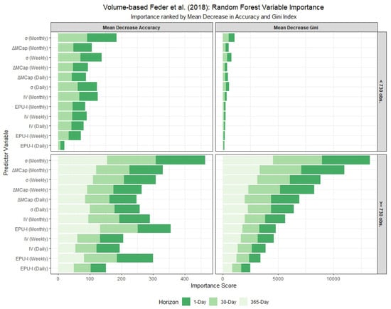
Figure 8.
In-sample variable importance from the Random Forest model, using the volume-based Feder et al. (2018) definition of failure. The plots show results for stablecoins with fewer (<730) and more (≥730) observations across different forecast horizons. Importance is measured by Mean Decrease in Accuracy (MDA, higher is better) and Mean Decrease in Gini (MDG, higher is better). Variables are ranked by MDA, highlighting the most predictive features for each group and horizon under this failure definition.
Detailed tabular results are available in the Appendix A. Panel model coefficient estimates are presented in Table A1 and Table A4 for stablecoins with ≥730 observations, and in Table A2 and Table A5 for those with fewer observations. Variable importance measures for the Random Forest models, covering both lifespan categories, are located in Table A3 and Table A6. The tables provide coefficient estimates for a suite of panel models (logit and cauchit variants with pooled, fixed effects (FE), bias-corrected FE, conditional logit, and random effects (RE) specifications) and key variable importance metrics (Mean Decrease Accuracy and Mean Decrease Gini) for 1-day, 30-day, and 365-day forecast horizons where applicable. In the random forest model, ‘Mean Decrease Accuracy’ (MDA) measures the average reduction in out-of-bag prediction accuracy when a variable is permuted, indicating its contribution to classification performance. ‘Mean Decrease Gini’ (MDG) quantifies the total decrease in node impurity (using the Gini index) across all splits involving the variable, reflecting its importance in tree construction.
4.2.1. Differences Between the $0.80 Price Threshold and the Feder Method
For stablecoins with fewer than 730 observations, the panel models under the $0.80 price threshold method (Table A2) reveal a mix of significant and insignificant regressors, with varying signs and magnitudes. The monthly market capitalization change () and volatilities (, ) consistently show statistical significance across most models for the 1-day horizon, with coefficients indicating strong effects—generally negative for (i.e., an increase in market cap reduces the PD) and positive for the volatilities (highlighting increased credit risk). Bitcoin volatility () and the monthly Economic Policy Uncertainty Index () also exhibit significant negative impacts, suggesting that higher Bitcoin volatility and economic uncertainty influence stablecoin failure. In contrast, for stablecoins with 730 or more observations (Table A1), the results are more consistent across models and horizons. For instance, and remain highly significant with mostly negative and positive signs, respectively, and Bitcoin volatility terms (, ) are uniformly negative and significant. This suggests that longer data histories enhance the stability and reliability of coefficient estimates, likely due to reduced noise and greater statistical power.
Under the Feder et al. (2018) volume-based criterion, differences between the two stablecoin groups are similarly pronounced. For coins with fewer than 730 observations (Table A5), the 1-day horizon shows fewer significant regressors, with consistently negative and positive, while is significant only in the pooled logit. For coins with 730 or more observations (Table A4), the 1-day horizon highlights (positive sign) and (negative sign) as key drivers, with more regressors achieving significance across models (e.g., particularly with negative effects). The 365-day horizon further amplifies these effects, with showing large negative coefficients. The increased significance and magnitude for coins with longer histories suggest that the volume-based Feder criterion benefits from extended data, capturing prolonged low-volume periods more effectively than the price threshold method, which reacts to immediate price drops.
Summarizing, the results exhibit notable differences depending on the method used to define stablecoin failures. For the $0.80 price threshold, variables such as the lagged monthly market capitalization change () and monthly volatility () are consistently significant across most panel models, particularly for stablecoins with ≥730 observations. In contrast, the Feder method places greater emphasis on volatility measures, with and showing strong predictive power. The Feder method also highlights the importance of economic policy uncertainty (), which is less pronounced in the price threshold analysis. This suggests that the Feder method, which incorporates trading volume, may capture broader market dynamics and systemic risks, while the price threshold focuses more on direct price declines.
4.2.2. Panel Models vs. Random Forest Models
Comparing panel models to random forest models reveals distinct interpretive strengths. Panel models (Table A1, Table A2, Table A4 and Table A5) provide coefficient estimates with statistical significance, allowing directional inference. For example, under the $0.80 threshold, has mainly a positive effect, implying that higher volatility increases the failure probability. Random forest models (Table A3 and Table A6), however, focus on variable importance via Mean Decrease Accuracy (MDA) and Mean Decrease Gini (MDG), without directional insight. For stablecoins with fewer than 730 observations (Table A3), tops the 1-day horizon for both criteria, followed by and , aligning with panel model significance but offering a non-parametric perspective.
Therefore, panel models and random forest approaches offer complementary insights. Panel models provide interpretable coefficients, revealing that lagged volatility and market capitalization changes are critical predictors. In contrast, random forest models prioritize variables based on predictive accuracy and Gini importance, with the stablecoin monthly volatility consistently ranking highest. This suggests that while panel models identify specific directional effects, random forest models capture non-linear relationships and interactions, particularly for volatility and market-derived variables.
4.2.3. Differences Across Forecast Horizons and Stablecoin Lifespans
Differences across forecast horizons are evident in both model types. For the $0.80 threshold with 730 or more observations (Table A1), the 1-day horizon shows strong effects from (mainly positive) and (mainly negative), which persist but weaken in magnitude at 30 days and further diminish at 365 days. This attenuation suggests that short-term volatility and market dynamics are more predictive of immediate failure, while longer horizons dilute these effects. For fewer than 730 observations (Table A2), the 30-day horizon shows fewer significant terms compared to the 1-day, indicating limited predictive power with shorter data spans. Random forest results (Table A3) mirror this, with MDA values for slightly decreasing from the 1-day to the 30-day horizon for stablecoins with fewer observations but remaining stable for those with longer histories, suggesting robustness across horizons when data is sufficient.
Under the Feder criterion, horizon effects differ. For 730 or more observations (Table A4), the 365-day horizon introduces more significant terms compared to the 1-day, reflecting the criterion’s sensitivity to prolonged low volume. For fewer observations (Table A5), the 30-day horizon shows reduced significance, likely due to data constraints. Random forest results (Table A6) confirm as the top predictor across all horizons, with and gaining importance at longer horizons, highlighting their role in sustained volume-based failure.
Summarizing, the forecast horizon significantly influences the results. For 1-day-ahead forecasts, daily and weekly variables play a more prominent role, while longer horizons (30-day and 365-day) emphasize monthly variables. The random forest results align with this pattern, showing higher importance scores for monthly variables at longer horizons. This indicates that short-term failures are driven by recent market movements, while long-term failures are influenced by sustained trends in volatility and market capitalization, as well as macroeconomic and systemic factors. Moreover, forecast horizon differences underscore short-term sensitivity in the $0.80 threshold and longer-term relevance in the Feder criterion, informing their suitability for different monitoring contexts.
Finally, we remark that stablecoins with 730 or more observations yield more robust and significant results across both forecasting models and definitions of stablecoin death, benefiting from longer data histories. These stablecoins exhibit more stable and statistically significant coefficients, particularly for monthly variables such as and . For these variables, the panel models consistently show strong negative coefficients for , indicating that declines in market capitalization are a robust predictor of failure, and positive coefficients for , suggesting that increases in stablecoin volatility are a reliable signal of impending failure. In contrast, stablecoins with fewer than 730 observations display more erratic results, with fewer significant coefficients and larger standard errors, likely due to limited data availability. The random forest results corroborate this evidence, showing higher variable importance scores for and in the larger dataset, further underscoring their reliability as predictors for more established stablecoins.
4.2.4. Economic Interpretation of In-Sample Drivers of Stablecoin Default
The in-sample results, consistently across model specifications, forecast horizons, sample lengths, and death definitions, reveal a coherent economic narrative linking market stability, investor confidence, and systemic trust mechanisms within the stablecoin ecosystem. Beyond statistical relationships, the estimated coefficients highlight how macro-financial and crypto-specific forces jointly determine the credibility and resilience of individual stablecoins.
First, the negative and highly significant effect of stablecoin volatility on the probability of default underscores the central role of price stability as a coordination device. In theoretical terms, lower volatility reduces uncertainty about redemption value and reinforces expectations of convertibility, which in turn strengthens the self-fulfilling confidence loop sustaining the peg. This finding is consistent with models of monetary trust and coordination equilibria, where small deviations from parity are tolerated, but increasing fluctuations erode collective confidence and trigger runs or liquidity withdrawals. Across model types, this effect remains the most robust determinant of survival, particularly at shorter forecast horizons, indicating that day-to-day price discipline is essential for maintaining the perception of “moneyness” [3,41]. For example, when significant volatility emerges for algorithmic stablecoins, this could indicate a breakdown in the arbitrage incentives designed to correct price deviations [3]. For collateralized stablecoins, it may reflect mounting concerns over the quality, liquidity, or transparency of the underlying reserves, raising redemption fears akin to a bank run [2]. High volatility deters a stablecoin’s use as a medium of exchange or unit of account within the decentralized finance (DeFi) ecosystem, eroding its utility and demand [4]. Consequently, elevated volatility is not merely a statistical feature but a direct symptom of a loss of monetary confidence—the core of what defines a stablecoin’s failure—as seen in the TerraUSD collapse, where amplified fluctuations eroded trust and triggered systemic contagion [18]. Our models quantitatively confirm that periods of high price instability are strong leading indicators of a terminal loss of peg and its final demise.
Second, larger increases in market capitalization are associated with a lower probability of failure, confirming that market depth and adoption act as stabilizing forces. Expanding capitalization reflects growing transactional use, network effects, and greater distribution of coin holdings, all of which contribute to reducing idiosyncratic liquidity shocks (S&P Global Ratings, 2025). Conversely, a declining market cap reflects net outflows, capital flight, and a collapse in confidence. This can trigger a negative feedback loop: as investors redeem or sell their holdings, the reduced market cap makes the coin more susceptible to large trades and liquidity crises, further increasing its fragility. Therefore, from an economic standpoint, higher capitalization signals stronger user trust and institutional anchoring, mitigating the risk of destabilizing redemptions. Interestingly, this protective effect becomes more pronounced in models estimated on longer time series (over 730 observations), where structural market expansion rather than short-term speculative inflows appears to drive stability. This distinction highlights how the accumulation of user base and transactional liquidity operates as a form of endogenous insurance for the peg (see [42,43]).
Third, a more nuanced finding is the generally negative relationship between Bitcoin’s implied volatility () and stablecoin default risk. At first glance, one might expect that turmoil in the core crypto asset (Bitcoin) would spill over and destabilize the entire ecosystem, including stablecoins. However, the negative coefficient suggests the opposite: when Bitcoin becomes more volatile, stablecoins appear to become safer in a relative sense. This admits a compelling economic interpretation as a flight-to-quality or flight-to-safety phenomenon within the digital asset space. During periods of extreme uncertainty and price swings in the crypto market, investors seek to de-risk their portfolios. They often divest from volatile assets like Bitcoin and Ethereum and park their capital in stablecoins to preserve value and await clearer market directions. This surge in demand for stability can temporarily bolster stablecoin prices, increase their trading volumes, and reduce their perceived default risk. This effect positions certain stablecoins as a type of “safe haven” asset within the crypto ecosystem—a role that becomes particularly prominent during internal market crises, even if they remain risky from a traditional finance perspective. This inverse relationship, consistent across almost all our models, underscores that stablecoin stability cannot be analyzed in isolation but must be viewed as embedded within the larger crypto-financial network (see [44,45,46,47,48]).
Finally, the role of the Economic Policy Uncertainty Index (EPU-I) is less dominant than the coin-specific factors, and its effect varies. However, when significant, it often carries a negative sign, implying that higher traditional economic uncertainty is associated with lower stablecoin default risk. In periods of heightened policy uncertainty, investors and institutions may increase their use of stablecoins as settlement or collateral instruments that combine the benefits of digital liquidity with perceived U.S. dollar stability. This effect is consistent with the safe-haven hypothesis observed for other dollar-denominated instruments: when traditional financial markets become riskier or regulatory uncertainty rises, stablecoins (particularly asset-backed designs) gain attractiveness as alternative transactional media. Conversely, during tranquil periods of low EPU, demand for stablecoins as a hedging or reserve instrument diminishes, potentially amplifying idiosyncratic fragility. This finding highlights the hybrid nature of stablecoins as both crypto assets and synthetic money-like instruments whose demand is countercyclical to global uncertainty (see [49,50,51,52]). However, the varying significance across models indicates that while EPU-I plays a role, coin-specific factors dominate, consistent with SP’s emphasis on internal reserve quality over external shocks [12].
When interpreted jointly, these results reveal a unified mechanism: stablecoin survival depends on the interaction between micro-level stability signals (volatility and capitalization) and macro-level credibility anchors (crypto and policy uncertainty). The consistency of these relationships across model types, forecast horizons, and definitions of failure suggests that the identified determinants reflect fundamental economic forces rather than model-specific artifacts. At a conceptual level, the evidence supports the view that stablecoins operate as endogenous confidence assets, sustained by liquidity, predictability, and systemic calm, whose failure dynamics mirror those of traditional monetary systems when the equilibrium of trust collapses. For investors, these insights advocate monitoring capitalization and volatility as early indicators, while regulators can leverage them to mitigate systemic risks, as warned by the Financial Stability Oversight Council (2024) [1]. Future research could extend this by incorporating real-time reserve data to refine these interpretations.
4.3. Out-of-Sample Analysis
We assess the forecasting performance of our eight panel models and the random forest model in detecting stablecoin failures, using both the $0.80 price threshold and the volume-based criterion of [5], as outlined in Section 3.1.
The initial dataset for estimating panel models and the Random Forest model spanned February 2021 to February 2022 for coins with fewer than 730 observations and January 2019 to January 2021 for coins with more than 730 observations. In essence, all stablecoin data were pooled together up to a specific time point (e.g., time t), and panel models along with the Random Forest model were estimated with this dataset to calculate the out-of-sample probabilities of death. Subsequently, the time window was extended by one day, and the process was repeated. For both the panel models and the Random Forest model, direct forecasts were generated by estimating the models multiple times, corresponding to the number of forecast horizons, using regressors lagged by the duration of each forecast horizon (e.g., 1-day lagged regressors for 1-day-ahead probability of death predictions, and so forth).
The out-of-sample performance of nine different models, tested under the two competing definitions of a stablecoin death, is visualized in Figure 9 and Figure 10. The plots evaluate performance using the AUC, H-measure, and Brier Score, segmenting the results by the stablecoin’s lifespan and the forecasting horizon. Models that are included in the Model Confidence Set (MCS), which is based on the Brier Score as a loss function at a 10% significance level, are highlighted with a solid point to denote them as statistically superior forecasting models. Detailed forecasting results are presented in tabular format in the Appendix A. Table A7 and Table A8 provide a comprehensive breakdown of performance, evaluated separately by stablecoin lifespan (<730 observations and ≥730 observations) and forecast horizon (1-day, 30-day, and 365-day, with the 365-day horizon applied only to stablecoins with longer histories). The tables include the aforementioned performance metrics (AUC, H-measure, Brier Score) along with standard classification metrics—Accuracy, Sensitivity, and Specificity—derived using two alternative thresholds (50% and empirical prevalence). Finally, the tables explicitly report each model’s inclusion in the Model Confidence Set.
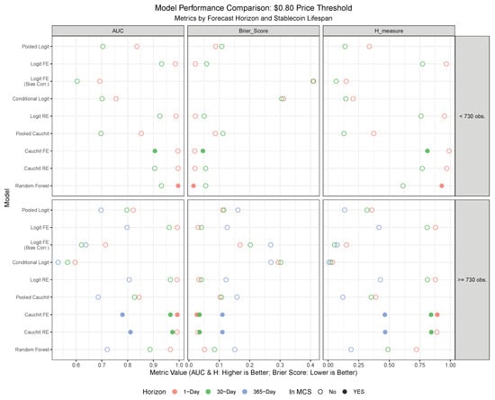
Figure 9.
Out-of-sample forecasting performance of nine models using the $0.80 price threshold definition of failure. Results are grouped by stablecoin lifespan (<730 and ≥730 observations) and forecast horizon (1-day, 30-day, 365-day). Performance is measured by the Area Under the Curve (AUC) and H-measure (where higher is better) and the Brier Score (where lower is better). Models marked with a solid point are included in the Model Confidence Set (MCS), indicating they are statistically among the best-performing models based on the Brier Score.
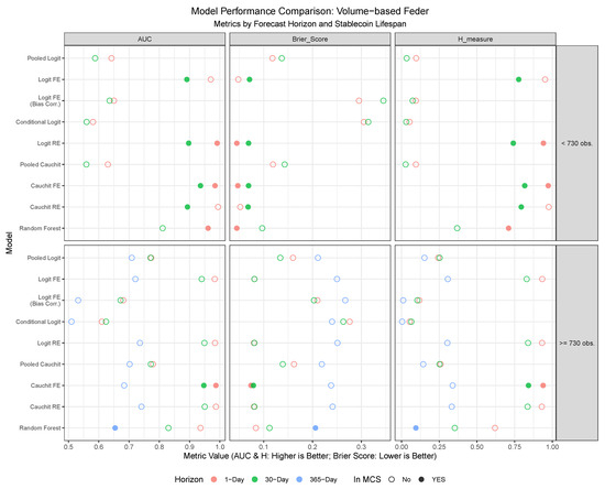
Figure 10.
Out-of-sample forecasting performance of nine models using the volume-based Feder et al. (2018) definition of failure. Results are grouped by stablecoin lifespan (<730 and ≥730 observations) and forecast horizon (1-day, 30-day, 365-day). Performance is measured by the Area Under the Curve (AUC) and H-measure (where higher is better) and the Brier Score (where lower is better). Models marked with a solid point are included in the Model Confidence Set (MCS), indicating they are statistically among the best-performing models based on the Brier Score.
Among the evaluated forecasting models, the panel Cauchit model with fixed effects consistently emerges as the top performer across multiple evaluation criteria, forecast horizons, and stablecoin classifications. This model demonstrates superior predictive power, as evidenced by its frequent inclusion in the Model Confidence Set (MCS), its consistently high AUC and H-measure values, and its low Brier Scores under both the $0.80 price threshold and the volume-based Feder approach. Particularly noteworthy is its robustness at shorter forecast horizons, where it achieves near-optimal sensitivity and specificity, making it highly reliable for real-time failure detection. For stablecoins with fewer than 730 observations, the panel Cauchit FE model excels in navigating volatility and limited data availability, while for longer-lived stablecoins, it leverages historical patterns to maintain strong performance. While other models, such as Random Forest and Logit RE, also perform well in specific contexts—particularly for short-term forecasts of stablecoins with fewer than 730 observations—their results are less consistent compared to the panel Cauchit FE model. In contrast, the bias-corrected logit model with fixed effects and the Conditional Logit model consistently underperform across both classification criteria, likely due to overfitting or misspecification in sparse data settings.
Based on these findings, the Cauchit FE model clearly emerges as the preferred choice for predicting stablecoin failures, particularly when aiming for a balance between accuracy, adaptability, and robustness across varying conditions.
In terms of differences among classification criteria, under the $0.80 price threshold (Table A7), models generally exhibit higher predictive power compared to the Feder criterion (Table A8), as evidenced by higher AUC and H-measure values across most horizons and lifespans. In contrast, the volume-based Feder approach incorporates trading volume dynamics, introducing additional complexity and noise into the classification process. Consequently, models evaluated under this criterion exhibit lower sensitivity and specificity, particularly at shorter forecast horizons, reflecting the inherent challenges of capturing failure events based on volume fluctuations.
The distinction between stablecoins with fewer than 730 observations and those with 730 or more observations also plays a significant role in shaping the results. Under the $0.80 threshold, stablecoins with fewer than 730 observations show excellent performance in short-term forecasts, particularly at the 1-day-ahead horizon. For stablecoins with 730 or more observations, performance remains strong, but sensitivity is generally lower, suggesting that longer histories dilute the ability to detect rare failure events amidst more stable periods. The Feder criterion generally mirrors this trend.
Across forecast horizons, predictive performance declines as the horizon extends, more markedly under the Feder criterion. This suggests that the $0.80 threshold retains more predictive power over longer horizons due to its focus on price signals, whereas the Feder criterion struggles as volume trends become less informative over time. Notably, models such as Logit RE and Cauchit RE maintain relatively strong performance across horizons for stablecoins with longer lifespans, underscoring their adaptability to varying forecasting requirements, even though they are considerably more difficult to estimate and computationally demanding.
In summary, based on these findings, we recommend the panel Cauchit FE model as the preferred choice for predicting stablecoin failures, particularly when aiming for a balance between accuracy, adaptability, and robustness across varying conditions. For applications where interpretability is less critical, the Random Forest model offers a competitive alternative, especially for short-term forecasts. The $0.80 price threshold method appears to outperform the Feder criterion in out-of-sample forecasting, particularly for short-term horizons and stablecoins with shorter lifespans, due to its sensitivity to immediate price deviations. Stablecoins with fewer than 730 observations benefit from higher precision in short-term forecasts, while those with 730 or more observations show robust but less sensitive predictions. Forecasting performance degrades across horizons, more so under the Feder approach, where long-term volume signals weaken.
5. Robustness Checks
5.1. A Time Series-Based Method
The Zero Price Probability (ZPP) method, adapted from [6,14,24], was employed to estimate market-implied probabilities of default or “death” for stablecoins. Rather than relying on prices, the method uses market capitalization, which provides a more comprehensive metric by reflecting both price and circulating supply—offering a better gauge of market sentiment and stability compared to trading volume. The ZPP method estimates the probability that a stablecoin’s market capitalization will fall to zero within specified time horizons (1-day, 30-day, and 365-day ahead). It involves three steps: modelling changes in market capitalization using a conditional model, simulating multiple future trajectories, and calculating the probability of default as the proportion of simulations where market capitalization falls to zero. This approach allows for flexible distributions beyond the log-normal and accommodates truncated variables like market capitalization, making it a robust indicator of default risk. For further details, see [53]. We also tested the Cox Proportional Hazards model used in [6], but encountered several numerical instability issues, particularly for stablecoins with fewer than 730 observations, consistent with the problems discussed in [6]. For this reason, we did not include this model in our analysis. The investigation of survival-type models with shrinkage estimators for stablecoin credit risk is left for future research.
As a robustness check, we applied the ZPP method under the assumption that a stablecoin’s market capitalization follows a simple random walk [ZPP(RW)], making this approach suitable for coins with limited data availability. Unlike the panel models, the ZPP model was estimated individually for each stablecoin. Given the relatively short length of historical market capitalization time series, we adopted an initial estimation sample of 30 observations. In this robustness check, we applied the ZPP(RW) alongside the previous forecasting models and the two classification criteria: the $0.80 price threshold and the volume-based method of [5].
It is important to note that the datasets used to estimate the panel and random forest models differed from those used for the ZPP models. As a result, there were certain dates for which not all models produced forecasts. Consequently, the evaluation metrics reported in Table A9 and Table A10 in the Appendix A are based exclusively on the subset of dates for which forecasts from all models were simultaneously available.
Overall, the results indicate that while the ZPP(RW) model performs reasonably well in terms of AUC, it generally exhibits lower accuracy, sensitivity, and specificity compared to more sophisticated models, and often fails to be included in the Model Confidence Set (MCS). Under the $0.80 price threshold, the ZPP(RW) achieves moderate AUC values for 1-day and 30-day forecasts, but its performance deteriorates sharply for longer horizons. The volume-based [5] criterion yields even weaker ZPP(RW) results, reflecting the method’s sensitivity to the failure definition. In contrast, models such as the panel Cauchit FE and Random Forest consistently outperform the ZPP(RW) under both criteria, underscoring their robustness.
The ZPP(RW) model performs relatively better for stablecoins with shorter lifespans (fewer than 730 observations), likely due to fewer structural breaks. However, even in this case, it is outperformed by panel models with fixed effects.
Across forecast horizons, the predictive power of the ZPP(RW) declines markedly beyond short-term forecasts (1-day and 30-day ahead), reflecting its simplicity and inability to capture complex dynamics over longer periods. This limitation arises because more advanced ZPP variants incorporating GARCH models require 500–1000 observations for stable parameter estimation and cannot be reliably applied to most of our dataset. See the large simulation studies on GARCH models by [54,55] for further details.
While the ZPP(RW) is outperformed by more complex panel models, its simplicity translates into specific practical advantages where sophisticated modelling is infeasible. This approach is particularly valuable in three scenarios:
- (a)
- Severe data scarcity: For a newly launched stablecoin or one with a very short trading history (e.g., less than 30-60 days), estimating panel models with multiple regressors or even a GARCH-based ZPP model is impossible. The ZPP(RW), requiring only a minimal initial window (e.g., 30 observations), provides a immediate, data-parsimonious method to generate an initial, market-implied PD estimate where no other model can run.
- (b)
- New stablecoin launches: Investors and exchanges listing a new stablecoin lack the coin-specific history needed for a fundamental credit assessment. In this vacuum, the ZPP(RW) can be applied from the first day of trading to monitor its market capitalization trajectory, offering a purely market-based, real-time signal of initial stability or distress that complements other due diligence.
- (c)
- Real-time monitoring and baselining: The computational simplicity of the ZPP(RW) allows it to be updated and calculated instantaneously with new market data. This makes it suitable for building real-time dashboards that monitor a large universe of stablecoins. It can serve as a high-level baseline alert system; if the ZPP(RW) for a coin spikes, it can trigger a deeper, more resource-intensive analysis using the superior panel Cauchit FE model.
In essence, the ZPP(RW) should not be seen as a competitor to the panel models but as a complementary tool for early-stage, resource-constrained, or high-frequency monitoring situations. It embodies a trade-off, sacrificing predictive power for immediacy and applicability in data-scarce environments.
In conclusion, while the ZPP(RW) offers a viable benchmark for short-term forecasts with minimal data requirements, its simplicity comes at the cost of lower accuracy—particularly for longer horizons or more complex failure definitions. These results reinforce the superiority of structured models such as the panel Cauchit model with fixed effects and highlight the trade-off between simplicity and predictive power in small-sample settings.
5.2. Alternative Sample Cutoff at 365 Observations
In our baseline analysis, we adopted a cutoff of 730 observations for stablecoin time series to ensure sufficient data for forecasting 365-day ahead probabilities of stablecoin death. This cutoff was chosen because it allows for a minimum of one year of training data for model initialization, with an additional year to evaluate forecasting performance, ensuring robust model training and reliable long-term predictions. To assess the robustness of our findings to the choice of sample size cutoff, we conducted an additional analysis using a smaller cutoff of 365 observations. This alternative cutoff aligns with standard practices in financial time series analysis, where a one-year period is often sufficient to capture meaningful patterns while including a broader set of stablecoins with shorter histories. We applied this alternative cutoff to both panel models and Random Forest models, using both the $0.80 price threshold approach and the volume-based Feder et al. (2018) methodology, as presented in Table A2, Table A3, Table A4, Table A5, Table A6, Table A11, Table A12 and Table A13. Below, we discuss the key findings from comparing the results for stablecoins with fewer than 730 observations versus fewer than 365 observations.
In the panel models (Table A2 and Table A11), the results for both cutoffs confirm the importance of monthly variables, particularly monthly volatility (), monthly market capitalization changes (), and monthly Bitcoin implied volatility (), which are significant across most models for both 1-day and 30-day ahead forecasts. However, the smaller 365-observation sample (Table A11) exhibits larger and more volatile coefficient estimates, especially in fixed effects (FE) and random effects (RE) models. For instance, in the 1-day ahead forecast, has coefficients of −222.158*** in Logit FE and −32.471 in Cauchit RE for the 365-observation sample, compared to −70.313*** and −41.741 in the 730-observation sample. This suggests increased sensitivity to data limitations or outliers in the smaller sample. Additionally, weekly volatility () is more significant in the 365-observation sample for the 1-day forecast, while economic uncertainty () gains prominence in the 30-day forecast, indicating that shorter samples may amplify certain effects. Similarly, in the volume-based Feder et al. (2018) panel models (Table A5 and Table A12), monthly variables remain dominant predictors. The 365-observation sample (Table A12) shows significantly larger coefficients for , such as −410.578*** in Logit FE and −1126.429*** in Cauchit FE for the 1-day forecast, compared to −6.279 and −3.702 in the 730-observation sample. The smaller sample also reverses the sign of in FE models (e.g., −0.901*** vs. 0.280*** in Logit FE), suggesting potential overfitting or data-specific effects. Weekly economic uncertainty () is more significant in the smaller sample for the 30-day forecast, further highlighting the sensitivity of shorter time series to specific variables.
In the Random Forest models (Table A3 and Table A13 for the $0.80 price threshold approach, and Table A6 and Table A13 for the Feder et al. approach), monthly variables (, , ) consistently rank among the top predictors for both cutoffs and forecast horizons. However, the 730-observation sample (Table A3 and Table A6) yields higher Mean Decrease in Accuracy and Mean Decrease in Gini values, indicating greater model robustness with larger datasets. For example, in the Random Forest model for the $0.80 price threshold approach, has an M.D. Accuracy of 71.59 and M.D. Gini of 462.49 for the 1-day forecast in the 730-observation sample, compared to 51.218 and 197.714 in the 365-observation sample. Similarly, in the Feder et al. approach, has an M.D. Accuracy of 92.731 and M.D. Gini of 532.785 in the 730-observation sample, versus 55.495 and 100.240 in the 365-observation sample. The smaller 365-observation sample elevates the relative importance of certain variables, such as and in the $0.80 price threshold approach, and and in the Feder et al. approach, particularly for the 1-day forecast. Weekly volatility () is more prominent in the 730-observation sample, especially in the Feder et al. approach, where it ranks second for both forecast horizons. These differences suggest that smaller samples may emphasize financial and economic indicators over volatility measures due to data constraints.
The robustness check using a 365-observation cutoff confirms that our primary findings are not overly sensitive to the choice of sample size, as monthly variables remain the most consistent predictors across both cutoffs, methodologies, and forecast horizons. The 730-observation cutoff, designed to support 365-day ahead forecasting with sufficient training data, provides more stable coefficient estimates in panel models and higher importance scores in Random Forest models, reflecting greater robustness with larger datasets. In contrast, the smaller 365-observation sample produces larger and more volatile coefficients in panel models and lower importance scores in Random Forest models, indicating potential overfitting or increased sensitivity to data limitations. These results highlight the trade-off between including more stablecoins with shorter histories and maintaining model stability with larger datasets. By presenting results for both cutoffs, we provide a comprehensive view of how sample size influences predictive performance, reinforcing the reliability of our conclusions.
6. Discussion and Conclusions
This study advances the understanding of stablecoin credit risk by introducing a novel rule-of-thumb approach to classify stablecoins as “dead” or “alive” using a $0.80 price threshold, validated against CoinMarketCap delistings and the volume-based methodology of [5]. The $0.80 threshold proved to be a robust and practical indicator of stablecoin failure, offering a real-time, transparent alternative to lagging indicators such as delistings or volume-based methods. Sensitivity analyses confirmed its balanced trade-off between detecting failures and preserving accuracy for surviving coins.
Employing a comprehensive dataset of 98 stablecoins, we utilized a suite of panel binary models and a random forest model to forecast probabilities of default (PDs), revealing that lagged monthly market capitalization () and stablecoin volatility () are the most significant predictors across both in-sample and out-of-sample analyses. The panel Cauchit model with fixed effects (Cauchit FE) consistently outperformed alternative specifications, achieving high AUC and H-measure values while remaining robust across forecast horizons and failure criteria. Random forest models complemented these findings, likewise ranking and as the top variables. In contrast, other factors such as Bitcoin implied volatility and economic policy uncertainty indices played a secondary role, underscoring the primacy of stablecoin-specific dynamics in stablecoin stability.
The in-sample results reveal that stablecoin survival is not random but driven by identifiable and economically meaningful forces. The empirical evidence shows that lower price volatility and larger market capitalization significantly reduce default risk, confirming that internal stability and scale are key to maintaining investor trust and transactional credibility. At the same time, the counterintuitive negative relationships between Bitcoin implied volatility and the Economic Policy Uncertainty Index with the probability of death indicate that stablecoins tend to benefit from periods of heightened uncertainty, functioning as relative safe havens within both the crypto ecosystem and the broader financial landscape. These findings emphasize that stablecoins operate at the intersection of micro-level market dynamics and macro-level confidence channels, behaving simultaneously as digital assets and synthetic money substitutes. From a policy perspective, the evidence highlights the importance of transparency in reserves and mechanisms that anchor redemption credibility, since these characteristics underpin stability across regimes. Future research could extend this framework by examining whether the same economic mechanisms apply to newer stablecoins or to those integrated into regulated payment systems, thereby testing the resilience of these relationships as the market and regulatory landscape evolve
The out-of-sample analysis further highlighted the superiority of the $0.80 threshold over the Feder criterion, particularly for short-term forecasts (1-day and 30-day), where the Cauchit FE and random forest models excelled. Stablecoins with fewer than 730 observations demonstrated higher precision in short-term predictions, likely due to reduced noise, while those with ≥730 observations exhibited robust performance but lower sensitivity, suggesting that longer time series dilute the ability to detect rare failure events amidst more stable periods. Model performance deteriorated over longer horizons, especially under the volume-based Feder method, as volume signals weakened. The robustness check using the Zero Price Probability with a random walk [ZPP(RW)] confirmed these general trends; however, this approach exhibited modest performance, limited by its simplicity and inability to capture complex dynamics, particularly beyond the 30-day forecast horizon.
The practical contributions of this study are directly applicable to financial regulators seeking to develop effective market surveillance tools. The simplicity and high accuracy of the $0.80 price threshold make it an ideal candidate for a first-tier, automated alert system to flag stablecoins experiencing acute distress. The TerraUSD collapse serves as a powerful case-study validation: had this framework been applied, the breach of the $0.80 threshold would have provided an unambiguous, real-time signal of its failure, far quicker than volume-based metrics or post-mortem delistings. Furthermore, our panel Cauchit FE model, which identified falling market capitalization and surging volatility as key predictors, would have shown a rapidly escalating probability of default (PD) in the days preceding the final de-peg. This demonstrates that regulators could use the price threshold for immediate triage and the panel model for more granular, forward-looking risk assessment, allowing for proactive intervention. Our findings thus provide a clear, data-driven roadmap for integrating stablecoin-specific risk factors into supervisory frameworks, consistent with the recommendations of the Financial Stability Oversight Council [1] and with S&P Global Ratings’ stablecoin assessment [12].
Despite its contributions, this study has limitations. The dataset, while extensive, may not capture all stablecoin failures due to missing data for delisted or obscure coins, potentially biasing results toward more prominent assets. The $0.80 threshold, though validated, is static and may not adapt to evolving market conditions or stablecoin designs (e.g., algorithmic vs. fiat-backed). Moreover, while the current framework relies on an instantaneous price threshold to classify stablecoin failures, it does not explicitly account for the duration of a depegging episode. Incorporating time as an additional dimension could meaningfully refine the identification of persistent versus transient instability. For instance, a stablecoin might be classified as failed only after remaining below the $0.80 threshold for a sustained period (e.g., several consecutive days), thereby distinguishing short-lived volatility from a genuine loss of confidence. Such a duration-based extension would align with survival or hazard models commonly used in credit-risk analysis, where the persistence of distress carries more predictive information than momentary breaches [56]. Although implementing duration models proved numerically challenging with the current dataset, this represents a promising avenue for future research, offering a natural bridge between threshold-based classification and state-transition modelling to better capture the temporal dynamics of stablecoin failure. Besides, the ZPP(RW)’s poor performance reflects data constraints—most stablecoins lack the 1000+ observations required for advanced GARCH-based ZPP variants—limiting its utility as a benchmark. Additionally, unobserved heterogeneity beyond fixed effects (e.g., governance or blockchain-specific risks) may influence PDs, yet our models cannot fully account for these due to data limitations.
Future research could address these gaps by expanding the dataset to include emerging stablecoins and refining the threshold approach with dynamic or coin-specific cutoffs, possibly using machine learning to optimize thresholds in real time. Incorporating blockchain-level data (e.g., transaction volumes, smart contract activity) could enhance model precision by capturing governance or operational risks absent from market-based regressors. Extending the ZPP framework with alternative time series models suited for small samples (e.g., Bayesian methods) could improve its performance with stablecoins exhibiting limited time series. Finally, exploring the interplay between stablecoin credit risk and DeFi ecosystem dynamics—such as liquidity pool dependencies—offers a promising avenue to assess systemic implications, building on [2,4]. Together, these efforts would refine the predictive tools and theoretical insights needed to navigate the evolving stablecoin landscape.
Funding
The author gratefully acknowledges financial support from the grant of the Russian Science Foundation n. 25-18-00319.
Data Availability Statement
The data are available from the authors upon request.
Acknowledgments
During the preparation of this manuscript, the author used Grok 4 for proofreading the written English. The author has reviewed and edited the output and takes full responsibility for the content of this publication.
Conflicts of Interest
The author declares no conflicts of interest.
Appendix A
Table A1.
$0.80 Price threshold: in-sample coefficient estimates for Panel models. The regressors are lagged according to the forecast horizon used for the direct forecasts. Stablecoins with ≥730 observations. Regressors lagged according to forecast horizon.
Table A1.
$0.80 Price threshold: in-sample coefficient estimates for Panel models. The regressors are lagged according to the forecast horizon used for the direct forecasts. Stablecoins with ≥730 observations. Regressors lagged according to forecast horizon.
| 1-DAY AHEAD FORECAST | ||||||||
| Pooled Logit | Logit FE | Logit FE (Bias Corr) | Conditional Logit | Logit RE | Pooled Cauchit | Cauchit FE | Cauchit RE | |
| −0.006 | 0.169 ** | 0.003 | −0.004 | 0.162 ** | −0.024 | 0.663 *** | 0.563 * | |
| −0.016 | −0.226 *** | −0.012 | −0.001 | −0.218 *** | −0.022 | −0.704 | −0.312 | |
| −0.089 *** | −1.483 *** | −0.276 *** | −0.066 *** | −1.417 *** | −0.136 * | −5.889 *** | −4.673 *** | |
| 0.110 *** | 0.053 * | 0.066 | 0.005 | 0.053 * | 0.072 | 0.996 *** | 0.006 | |
| 0.397 *** | 0.115 *** | 0.331 *** | 0.029 *** | 0.115 *** | 0.470 *** | 0.608 *** | −0.118 | |
| 1.164 *** | 0.187 *** | 0.156 *** | 0.081 *** | 0.187 *** | 5.744 *** | 2.145 *** | 5.349 *** | |
| −0.150 ** | −0.561 *** | −0.165 * | −0.198 *** | −0.562 *** | −0.502 *** | −1.067 *** | −0.993 *** | |
| 0.150 * | 0.690 *** | 0.210 * | 0.181 ** | 0.690 *** | 0.291 * | 0.439 * | 0.434 * | |
| −0.390 *** | −1.669 *** | −0.470 *** | −0.484 *** | −1.665 *** | −0.984 *** | −2.718 *** | −2.805 *** | |
| 0.001 | 0.017 | 0.001 | 0.003 | 0.017 | 0.003 | 0.030 | 0.039 | |
| −0.023 | −0.034 | −0.028 | 0.011 | −0.034 | 0.004 | 0.155 | 0.164 | |
| −0.217 *** | −1.236 *** | −0.305 *** | −0.282 *** | −1.231 *** | −1.041 *** | −2.610 *** | −2.491 *** | |
| 30-DAY AHEAD FORECAST | ||||||||
| Pooled Logit | Logit FE | Logit FE (Bias Corr) | Conditional Logit | Logit RE | Pooled Cauchit | Cauchit FE | Cauchit RE | |
| − 0.011 | −0.015 | −0.007 | −0.013 | −0.016 | −0.040 | −0.075 | −0.081 | |
| −0.020 | −0.067 | −0.006 | 0.000 | −0.069 | −0.028 | 0.161 | 0.178 | |
| −0.078 *** | −0.985 *** | −0.268 *** | −0.062 *** | −0.954 *** | −0.105 | −1.144 *** | −1.151 *** | |
| 0.054 * | 0.016 | −0.021 | 0.003 | 0.016 | 0.113 * | 0.059 | 0.111 * | |
| 0.036 | 0.039 | 0.007 | 0.013 | 0.039 | −0.338 *** | −0.015 | −0.205 ** | |
| 1.275 *** | 0.176 *** | 0.248 *** | 0.080 *** | 0.176 *** | 5.843 *** | 2.469 *** | 2.534 *** | |
| −0.162 ** | −0.672 *** | −0.193 ** | −0.216 *** | −0.672 *** | −0.473 *** | −1.753 *** | −1.746 *** | |
| 0.128 * | 0.585 *** | 0.194 * | 0.170 ** | 0.584 *** | 0.139 | 1.320 *** | 1.346 *** | |
| −0.373 *** | −1.536 *** | −0.464 *** | −0.456 *** | −1.533 *** | −0.889 *** | −3.157 *** | −3.166 *** | |
| −0.000 | 0.006 | −0.000 | 0.002 | 0.006 | −0.010 | 0.007 | 0.008 | |
| −0.041 | −0.135 * | −0.054 | −0.017 | −0.135 * | −0.045 | −0.034 | −0.041 | |
| −0.175 *** | −1.204 *** | −0.280 *** | −0.287 *** | −1.199 *** | −0.867 *** | −2.605 *** | −2.564 *** | |
| 365-DAY AHEAD FORECAST | ||||||||
| Pooled Logit | Logit FE | Logit FE (Bias Corr) | Conditional Logit | Logit RE | Pooled Cauchit | Cauchit FE | Cauchit RE | |
| −0.004 | −0.001 | −0.001 | −0.002 | −0.001 | −0.017 | −0.005 | −0.005 | |
| −0.013 | 0.015 | 0.030 | 0.003 | 0.015 | −0.049 * | 0.049 | 0.049 | |
| −0.018 | −0.041 | −0.136 *** | −0.019 | −0.041 | 0.037 | −0.109 * | −0.109 * | |
| 0.024 | −0.010 | −0.014 | −0.002 | −0.010 | −0.038 | −0.030 | −0.030 | |
| 0.021 | −0.033 | −0.034 | −0.010 | −0.033 | −0.128 *** | −0.263 | −0.263 | |
| 0.515 *** | −0.197 *** | −0.860 *** | −0.036 * | −0.195 *** | 2.207 *** | −0.565 *** | −0.565 *** | |
| −0.176 *** | −0.650 *** | −0.238 *** | −0.205 *** | −0.649 *** | −0.381 *** | −1.440 *** | −1.440 *** | |
| 0.056 | 0.154 | 0.118 | 0.070 | 0.153 | 0.059 | 0.418 * | 0.418 * | |
| −0.266 *** | −0.955 *** | −0.395 *** | −0.313 *** | −0.953 *** | −0.486 *** | −2.141 *** | −2.141 *** | |
| 0.005 | −0.000 | −0.004 | 0.004 | −0.000 | 0.032 | 0.015 | 0.015 | |
| 0.014 | −0.034 | −0.054 | −0.009 | −0.033 | 0.080 | 0.046 | 0.046 | |
| −0.086 ** | −0.808 *** | −0.186 *** | −0.178 *** | −0.805 *** | −0.422 *** | −2.723 *** | −2.722 *** | |
*** for p-value < 0.001, ** for p-value < 0.01, * for p-value < 0.05.
Table A2.
$0.80 Price threshold: in-sample coefficient estimates for Panel models (no intercept). The regressors are lagged according to the forecast horizon used for the direct forecasts. Stablecoins with <730 observations. Regressors lagged according to forecast horizon.
Table A2.
$0.80 Price threshold: in-sample coefficient estimates for Panel models (no intercept). The regressors are lagged according to the forecast horizon used for the direct forecasts. Stablecoins with <730 observations. Regressors lagged according to forecast horizon.
| 1-DAY AHEAD FORECAST | ||||||||
| Pooled Logit | Logit FE | Logit FE (Bias Corr) | Conditional Logit | Logit RE | Pooled Cauchit | Cauchit FE | Cauchit RE | |
| −0.008 | 1.242 | 0.110 | 0.194 | 0.026 | −0.019 | 0.273 | 0.171 | |
| −0.007 | 1.321 | 0.390 | 2.201 | 0.400 | −0.024 | 4.687 | 5.251 | |
| −0.111 * | −70.313 *** | −4.258 | −16.821 ** | −0.770 | −0.187 | −46.821 | −41.741 | |
| 0.069 | 0.010 | 0.057 | 0.011 | 0.014 | 0.306 ** | −0.003 | −0.003 | |
| 0.139 ** | 0.162 * | 0.130 * | 0.061 * | 0.159 ** | 1.483 *** | 0.191 * | 0.190 * | |
| 0.597 *** | 0.175 ** | 0.448 *** | 0.180 *** | 0.190 *** | 0.807 *** | 0.199 * | 0.201 * | |
| −0.065 | −0.658 *** | −0.085 | −0.236 ** | −0.668 *** | −1.114 *** | −1.659 *** | −1.654 *** | |
| −0.174 | 0.066 | −0.140 | 0.063 | 0.106 | 0.833 *** | 0.378 | 0.377 | |
| 0.119 | −2.164 *** | −0.026 | −0.789 *** | −2.096 *** | −0.258 | −5.621 *** | −5.608 *** | |
| −0.007 | −0.011 | −0.004 | −0.002 | 0.005 | 0.027 | 0.023 | 0.021 | |
| 0.077 | 0.306 *** | 0.083 | 0.107 ** | 0.308 *** | 0.056 | 0.285 * | 0.289 * | |
| 0.233 *** | −0.801 *** | 0.168 ** | −0.141 *** | −0.794 *** | 0.456 *** | −1.260 *** | −1.258 *** | |
| 30-DAY AHEAD FORECAST | ||||||||
| Pooled Logit | Logit FE | Logit FE (Bias Corr) | Conditional Logit | Logit RE | Pooled Cauchit | Cauchit FE | Cauchit RE | |
| −0.008 | −0.236 | −0.059 | −0.257 | 0.032 | −0.018 | −0.296 | −0.241 | |
| −0.008 | 1.698 | 0.019 | 1.492 | 0.234 | −0.015 | 1.425 | 1.377 | |
| −0.115 * | 6.939 | 1.514 | 8.686 | −0.191 | −0.154 | 25.446 | 21.860 | |
| 0.056 | 0.011 | 0.041 | 0.012 | 0.012 | 1.840 *** | 0.003 | 0.004 | |
| 0.028 | −0.101 | 0.000 | −0.033 | −0.101 | 0.080 | −0.395 *** | −0.400 *** | |
| 0.593 *** | 0.231 *** | 0.498 *** | 0.184 *** | 0.231 *** | 0.804 *** | 0.304 *** | 0.305 *** | |
| −0.055 | −0.842 *** | −0.093 | −0.265 ** | −0.830 *** | −0.685 ** | −1.380 *** | −1.377 *** | |
| −0.453 ** | −0.321 | −0.397 * | −0.258 * | −0.329 | −0.360 | −0.261 | −0.262 | |
| 0.439 *** | −0.984 *** | 0.292 ** | −0.307 *** | −0.977 *** | 0.453 ** | −2.478 *** | −2.473 *** | |
| −0.007 | −0.022 | −0.007 | −0.009 | −0.023 | 0.003 | 0.008 | 0.009 | |
| 0.045 | −0.051 | 0.033 | −0.037 | −0.051 | 0.034 | −0.112 | −0.114 | |
| 0.179 *** | −0.582 *** | 0.128 * | −0.109 ** | −0.576 *** | 0.271 *** | −1.013 *** | −1.012 *** | |
*** for p-value < 0.001, ** for p-value < 0.01, * for p-value < 0.05.
Table A3.
$0.80 Price threshold: Random Forest variable importance measures. The variables are sorted in decreasing order according to the Out-Of-Bag accuracy for each forecasting horizon. Regressors lagged according to forecast horizon.
Table A3.
$0.80 Price threshold: Random Forest variable importance measures. The variables are sorted in decreasing order according to the Out-Of-Bag accuracy for each forecasting horizon. Regressors lagged according to forecast horizon.
| Stablecoins with <730 observations. | ||||||||
| 1-DAY AHEAD FORECAST | 30-DAY AHEAD FORECAST | |||||||
| M.D. Accuracy | M.D. Gini | M.D. Accuracy | M.D. Gini | |||||
| 71.59 | 462.49 | 66.45 | 453.91 | |||||
| 55.31 | 334.60 | 53.86 | 326.27 | |||||
| 52.14 | 137.11 | 52.89 | 371.98 | |||||
| 47.55 | 243.89 | 50.90 | 258.33 | |||||
| 47.20 | 295.53 | 50.21 | 134.45 | |||||
| 43.21 | 348.89 | 49.29 | 276.18 | |||||
| 41.74 | 293.42 | 41.29 | 94.43 | |||||
| 41.35 | 75.08 | 41.00 | 110.23 | |||||
| 39.24 | 82.86 | 40.36 | 89.73 | |||||
| 38.55 | 63.55 | 39.41 | 195.03 | |||||
| 26.20 | 42.90 | 37.81 | 62.88 | |||||
| 9.05 | 30.92 | 14.30 | 37.26 | |||||
| Stablecoins with ≥730 observations. | ||||||||
| 1-DAY AHEAD FORECAST | 30-DAY AHEAD FORECAST | 365-DAY AHEAD FORECAST | ||||||
| M.D. Accuracy | M.D. Gini | M.D. Accuracy | M.D. Gini | M.D. Accuracy | M.D. Gini | |||
| 147.34 | 4170.00 | 148.36 | 4227.32 | 148.34 | 3380.54 | |||
| 114.78 | 1058.70 | 112.97 | 1067.48 | 132.88 | 2418.49 | |||
| 109.24 | 1296.23 | 108.88 | 1897.56 | 127.59 | 1191.95 | |||
| 101.63 | 1816.94 | 102.36 | 1331.41 | 105.25 | 1299.73 | |||
| 92.32 | 2801.37 | 95.58 | 2623.14 | 94.73 | 2263.76 | |||
| 92.26 | 2048.69 | 93.01 | 727.75 | 88.02 | 1655.30 | |||
| 89.60 | 700.83 | 89.36 | 1933.23 | 80.74 | 820.46 | |||
| 82.17 | 1018.08 | 77.90 | 1046.30 | 78.13 | 1295.40 | |||
| 72.72 | 1303.10 | 76.23 | 926.57 | 76.58 | 1682.79 | |||
| 72.64 | 898.06 | 73.03 | 1315.23 | 72.49 | 1079.72 | |||
| 60.84 | 1005.85 | 64.37 | 1008.46 | 60.93 | 938.19 | |||
| 37.58 | 479.25 | 44.30 | 494.27 | 49.36 | 530.11 | |||
Table A4.
Volume-based Feder et al. (2018): in-sample coefficient estimates for Panel models. The regressors are lagged according to the forecast horizon used for the direct forecasts. Stablecoins with ≥730 observations. Regressors lagged according to forecast horizon.
Table A4.
Volume-based Feder et al. (2018): in-sample coefficient estimates for Panel models. The regressors are lagged according to the forecast horizon used for the direct forecasts. Stablecoins with ≥730 observations. Regressors lagged according to forecast horizon.
| 1-DAY AHEAD FORECAST | ||||||||
| Pooled Logit | Logit FE | Logit FE (Bias Corr) | Conditional Logit | Logit RE | Pooled Cauchit | Cauchit FE | Cauchit RE | |
| −0.005 | −0.001 | −0.003 | 0.000 | −0.001 | −0.013 | −0.007 | −0.007 | |
| −0.013 | 0.008 | −0.015 | 0.007 | 0.007 | 0.040 | −0.072 | −0.071 | |
| −0.031 * | 0.066 ** | 0.003 | 0.013 | 0.066 ** | −0.076 ** | 0.368 *** | 0.368 *** | |
| 0.031 | 0.022 | 0.015 | 0.001 | 0.022 | 0.047 | 0.123 * | 0.123 * | |
| −0.039 | −0.006 | −0.017 | 0.002 | −0.006 | −0.261 *** | −0.846 *** | −0.846 *** | |
| 1.150 *** | 0.290 *** | 0.539 *** | 0.048 *** | 0.291 *** | 3.706 *** | 3.515 *** | 3.515 *** | |
| −0.176 *** | −0.564 *** | −0.225 *** | −0.252 *** | −0.564 *** | −0.276 *** | −0.788 *** | −0.788 *** | |
| 0.076 | 0.350 *** | 0.120 | 0.155 *** | 0.349 *** | 0.030 | 0.420 *** | 0.420 *** | |
| −0.358 *** | −1.140 *** | −0.444 *** | −0.544 *** | −1.138 *** | −0.558 *** | −1.541 *** | −1.541 *** | |
| 0.002 | −0.000 | 0.001 | −0.001 | −0.000 | 0.004 | −0.000 | −0.000 | |
| −0.010 | −0.086 * | −0.021 | −0.015 | −0.085 * | −0.035 | −0.071 | −0.071 | |
| −0.035 | −0.538 *** | −0.084 ** | −0.153 *** | −0.537 *** | −0.079 * | −1.194 *** | −1.194 *** | |
| 30-DAY AHEAD FORECAST | ||||||||
| Pooled Logit | Logit FE | Logit FE (Bias Corr) | Conditional Logit | Logit RE | Pooled Cauchit | Cauchit FE | Cauchit RE | |
| −0.004 | −0.001 | −0.003 | −0.000 | −0.001 | −0.021 | −0.008 | −0.008 | |
| −0.016 | 0.001 | −0.018 | 0.003 | 0.001 | 0.042 * | −0.071 | −0.072 | |
| −0.025 | 0.076 ** | 0.010 | 0.020 | 0.076 ** | −0.070 * | 0.394 *** | 0.400 *** | |
| 0.048 | 0.030 | 0.024 | 0.002 | 0.030 | 0.094 * | −0.010 | −0.007 | |
| 0.012 | 0.029 | 0.013 | 0.008 | 0.029 | −0.242 *** | −0.228 *** | −0.234 *** | |
| 1.110 *** | 0.265 *** | 0.528 *** | 0.041 *** | 0.266 *** | 3.582 *** | 3.406 *** | 3.459 *** | |
| −0.192 *** | −0.570 *** | −0.238 *** | −0.260 *** | −0.569 *** | −0.301 *** | −0.733 *** | −0.732 *** | |
| 0.093 | 0.374 *** | 0.138 * | 0.168 *** | 0.373 *** | 0.047 | 0.472 *** | 0.470 *** | |
| −0.359 *** | −1.106 *** | −0.441 *** | −0.532 *** | −1.105 *** | −0.545 *** | −1.547 *** | −1.547 *** | |
| −0.000 | −0.007 | −0.002 | −0.004 | −0.007 | −0.003 | −0.010 | −0.010 | |
| −0.014 | −0.087 * | −0.025 | −0.011 | −0.086 * | −0.045 | −0.076 | −0.077 | |
| −0.031 | −0.499 *** | −0.078 ** | −0.165 *** | −0.497 *** | −0.079 * | −1.085 *** | −1.078 *** | |
| 365-DAY AHEAD FORECAST | ||||||||
| Pooled Logit | Logit FE | Logit FE (Bias Corr) | Conditional Logit | Logit RE | Pooled Cauchit | Cauchit FE | Cauchit RE | |
| −0.010 | 0.023 | −0.005 | −0.012 | 0.022 | −0.043 ** | −0.256 *** | −0.257 *** | |
| −0.015 | −0.040 | −0.017 | −0.002 | −0.044 | 0.001 | −0.813 *** | −0.810 *** | |
| −0.170 *** | −0.999 *** | −0.266 *** | −0.109 *** | −0.974 *** | −0.162 *** | −2.619 *** | −2.622 *** | |
| 0.010 | 0.004 | −0.002 | 0.000 | 0.004 | 0.055 | 0.009 | 0.009 | |
| −0.094 *** | −0.017 | −0.038 | −0.008 | −0.017 | −0.207 *** | −0.041 * | −0.041 * | |
| 1.347 *** | 0.073 *** | 0.467 *** | 0.026 *** | 0.074 *** | 2.563 *** | 0.233 *** | 0.233 *** | |
| −0.203 *** | −0.460 *** | −0.238 *** | −0.236 *** | −0.460 *** | −0.282 *** | −0.596 *** | −0.596 *** | |
| 0.077 | 0.252 *** | 0.118 * | 0.124 ** | 0.252 *** | 0.108 | 0.199 * | 0.199 * | |
| −0.396 *** | −0.909 *** | −0.449 *** | −0.479 *** | −0.908 *** | −0.602 *** | −1.176 *** | −1.177 *** | |
| −0.007 | −0.020 | −0.009 | −0.010 | −0.020 | −0.011 | −0.017 | −0.017 | |
| −0.035 | −0.093 * | −0.044 | −0.035 | −0.093 * | −0.086 * | −0.118 * | −0.118 * | |
| −0.175 *** | −0.347 *** | −0.169 *** | −0.162 *** | −0.347 *** | −0.233 *** | −0.988 *** | −0.989 *** | |
*** for p-value < 0.001, ** for p-value < 0.01, * for p-value < 0.05.
Table A5.
Volume-based Feder et al. (2018): in-sample coefficient estimates for Panel models (no intercept). The regressors are lagged according to the forecast horizon used for the direct forecasts. Stablecoins with <730 observations. Regressors lagged according to forecast horizon.
Table A5.
Volume-based Feder et al. (2018): in-sample coefficient estimates for Panel models (no intercept). The regressors are lagged according to the forecast horizon used for the direct forecasts. Stablecoins with <730 observations. Regressors lagged according to forecast horizon.
| 1-DAY AHEAD FORECAST | ||||||||
| Pooled Logit | Logit FE | Logit FE (Bias Corr) | Conditional Logit | Logit RE | Pooled Cauchit | Cauchit FE | Cauchit RE | |
| −0.007 | 0.367 | 0.270 | 0.234 | 0.057 | −0.011 | 0.183 | 0.184 | |
| −0.009 | −0.374 | −0.322 | −0.167 | −0.211 | −0.027 | −0.069 | −0.068 | |
| −0.121 ** | −6.279 | −4.466 | −4.274 | −0.450 | −0.122 | −3.702 | −3.731 | |
| −0.002 | 0.003 | 0.008 | 0.007 | 0.006 | −0.273 | 0.022 | 0.023 | |
| −0.300 *** | −0.306 *** | −0.227 *** | −0.228 *** | −0.298 *** | −0.760 *** | −0.234 ** | −0.233 ** | |
| 0.101 * | 0.280 *** | 0.248 *** | 0.212 *** | 0.276 *** | 0.341 *** | 0.409 *** | 0.409 *** | |
| 0.041 | −0.163 | −0.086 | −0.060 | −0.175 | 0.229 | −0.166 | −0.166 | |
| −0.146 | 0.195 | 0.118 | 0.048 | 0.196 | −0.412 | 0.217 | 0.217 | |
| −0.083 | −1.030 *** | −0.648 *** | −0.481 *** | −1.014 *** | −0.251 * | −1.303 *** | −1.303 *** | |
| −0.011 | −0.011 | −0.007 | −0.011 | −0.011 | −0.003 | 0.002 | 0.002 | |
| −0.016 | −0.017 | −0.015 | 0.025 | −0.015 | −0.053 | 0.022 | 0.022 | |
| 0.360 *** | −0.092 | −0.046 | 0.003 | −0.095 | 0.655 *** | −0.127 | −0.127 | |
| 30-DAY AHEAD FORECAST | ||||||||
| Pooled Logit | Logit FE | Logit FE (Bias Corr) | Conditional Logit | Logit RE | Pooled Cauchit | Cauchit FE | Cauchit RE | |
| −0.009 | 0.255 | 0.195 | 0.197 | −0.007 | −0.015 | 0.140 | 0.141 | |
| −0.012 | 0.005 | −0.051 | 0.107 | −0.135 | −0.027 | −0.035 | −0.033 | |
| −0.122 ** | −6.392 | −4.690 | −4.889 * | −0.488 | −0.122 | −4.147 | −4.184 | |
| 0.005 | 0.003 | 0.005 | 0.004 | 0.006 | −0.013 | 0.036 | 0.035 | |
| 0.007 | −0.011 | −0.006 | −0.010 | −0.001 | −0.044 | 0.067 | 0.068 | |
| −0.004 | 0.211 *** | 0.194 *** | 0.180 *** | 0.205 *** | 0.147 ** | 0.675 *** | 0.676 *** | |
| −0.003 | −0.361 * | −0.196 | −0.122 | −0.370 * | 0.116 | −0.359 | −0.359 | |
| −0.146 | 0.315 | 0.165 | 0.100 | 0.313 | −0.508 * | 0.299 | 0.300 | |
| −0.035 | −1.250 *** | −0.712 *** | −0.554 *** | −1.232 *** | −0.063 | −1.667 *** | −1.667 *** | |
| −0.012 | −0.055 | −0.028 | −0.025 | −0.055 | −0.010 | −0.083 | −0.083 | |
| 0.110 ** | 0.118 | 0.075 | 0.045 | 0.118 | 0.149 * | 0.206 * | 0.206 * | |
| 0.232 *** | −0.209 *** | −0.102 | −0.009 | −0.212 *** | 0.449 *** | −0.479 *** | −0.479 *** | |
*** for p-value < 0.001, ** for p-value < 0.01, * for p-value < 0.05.
Table A6.
Volume-based Feder et al. (2018): Random Forest variable importance measures. The variables are sorted in decreasing order according to the Out-Of-Bag accuracy for each forecasting horizon. Regressors lagged according to forecast horizon.
Table A6.
Volume-based Feder et al. (2018): Random Forest variable importance measures. The variables are sorted in decreasing order according to the Out-Of-Bag accuracy for each forecasting horizon. Regressors lagged according to forecast horizon.
| Stablecoins with <730 observations. | ||||||||
| 1-DAY AHEAD FORECAST | 30-DAY AHEAD FORECAST | |||||||
| M.D. Accuracy | M.D. Gini | M.D. Accuracy | M.D. Gini | |||||
| 92.731 | 532.785 | 91.517 | 527.257 | |||||
| 66.244 | 379.758 | 70.878 | 399.964 | |||||
| 60.904 | 284.065 | 67.102 | 187.943 | |||||
| 58.361 | 280.940 | 62.362 | 287.241 | |||||
| 57.882 | 174.456 | 48.519 | 272.206 | |||||
| 47.360 | 212.664 | 47.302 | 198.873 | |||||
| 45.059 | 132.145 | 45.488 | 134.969 | |||||
| 45.047 | 247.512 | 45.327 | 133.427 | |||||
| 40.069 | 120.647 | 43.199 | 225.551 | |||||
| 38.699 | 109.675 | 42.100 | 119.303 | |||||
| 37.374 | 96.648 | 34.062 | 96.868 | |||||
| 11.768 | 72.393 | 7.814 | 66.980 | |||||
| Stablecoins with ≥730 observations. | ||||||||
| 1-DAY AHEAD FORECAST | 30-DAY AHEAD FORECAST | 365-DAY AHEAD FORECAST | ||||||
| M.D. Accuracy | M.D. Gini | M.D. Accuracy | M.D. Gini | M.D. Accuracy | M.D. Gini | |||
| 156.038 | 4325.298 | 153.021 | 4402.147 | 154.711 | 4555.518 | |||
| 113.664 | 1057.233 | 118.101 | 1548.791 | 133.139 | 1769.350 | |||
| 104.507 | 1466.079 | 105.139 | 3733.134 | 120.479 | 3345.022 | |||
| 104.448 | 3895.016 | 103.306 | 1118.834 | 110.163 | 3133.867 | |||
| 100.646 | 2754.708 | 98.341 | 1838.324 | 99.865 | 2283.636 | |||
| 95.821 | 1786.739 | 97.645 | 2941.215 | 94.857 | 2001.125 | |||
| 88.308 | 3065.650 | 83.506 | 2858.668 | 91.542 | 2326.249 | |||
| 84.569 | 2582.196 | 78.018 | 2094.880 | 85.819 | 1978.278 | |||
| 79.606 | 2032.422 | 76.798 | 2373.704 | 81.943 | 1250.345 | |||
| 73.328 | 1456.258 | 71.111 | 1494.133 | 60.864 | 1655.588 | |||
| 72.889 | 1266.673 | 67.097 | 1279.382 | 54.564 | 1339.696 | |||
| 48.288 | 822.535 | 53.185 | 838.811 | 50.066 | 846.033 | |||
Table A7.
$0.80 Price threshold: AUC, H-measure, Brier scores, models included in the MCS, and evaluation metrics for all models using two alternative thresholds for converting probabilities into binary variables (50% and empirical prevalence). Results are separated by stablecoins lifespans and forecasting horizons for out-of-sample forecasts.
| Stablecoins with <730 observations. | ||||||||||
| 1-DAY AHEAD FORECAST | ||||||||||
| Model | AUC | H | Brier S. | Accuracy | Sensitivity | Specificity | Accuracy | Sensitivity | Specificity | MCS |
| Threshold: 50% | Threshold: empirical prevalence | |||||||||
| Pooled Logit | 0.836 | 0.338 | 0.088 | 0.890 | 0.095 | 0.990 | 0.416 | 0.983 | 0.345 | No |
| Logit FE | 0.985 | 0.967 | 0.021 | 0.973 | 0.775 | 0.998 | 0.990 | 0.921 | 0.998 | No |
| Logit FE (Bias. Corr.) | 0.692 | 0.148 | 0.408 | 0.481 | 0.954 | 0.422 | 0.137 | 1.000 | 0.029 | No |
| Conditional Logit | 0.755 | 0.204 | 0.311 | 0.450 | 0.919 | 0.391 | 0.151 | 1.000 | 0.045 | No |
| Logit RE | 0.988 | 0.951 | 0.021 | 0.973 | 0.770 | 0.999 | 0.990 | 0.922 | 0.999 | No |
| Pooled Cauchit | 0.853 | 0.373 | 0.087 | 0.891 | 0.277 | 0.969 | 0.458 | 0.993 | 0.390 | No |
| Cauchit FE | 0.995 | 0.989 | 0.019 | 0.976 | 0.790 | 0.999 | 0.988 | 0.899 | 0.999 | No |
| Cauchit RE | 0.996 | 0.970 | 0.020 | 0.976 | 0.793 | 0.999 | 0.988 | 0.900 | 0.999 | No |
| Random Forest | 0.996 | 0.929 | 0.015 | 0.986 | 0.909 | 0.995 | 0.908 | 0.995 | 0.897 | YES |
| 30-DAY AHEAD FORECAST | ||||||||||
| Model | AUC | H | Brier S. | Accuracy | Sensitivity | Specificity | Accuracy | Sensitivity | Specificity | MCS |
| Threshold: 50% | Threshold: empirical prevalence | |||||||||
| Pooled Logit | 0.704 | 0.138 | 0.108 | 0.871 | 0.086 | 0.980 | 0.427 | 0.915 | 0.358 | No |
| Logit FE | 0.932 | 0.772 | 0.058 | 0.931 | 0.523 | 0.988 | 0.954 | 0.718 | 0.987 | No |
| Logit FE (Bias. Corr.) | 0.604 | 0.066 | 0.410 | 0.451 | 0.801 | 0.402 | 0.150 | 0.995 | 0.032 | No |
| Conditional Logit | 0.701 | 0.145 | 0.305 | 0.493 | 0.811 | 0.448 | 0.195 | 0.995 | 0.084 | No |
| Logit RE | 0.925 | 0.760 | 0.050 | 0.938 | 0.528 | 0.995 | 0.960 | 0.719 | 0.994 | No |
| Pooled Cauchit | 0.697 | 0.130 | 0.112 | 0.865 | 0.140 | 0.966 | 0.427 | 0.884 | 0.363 | No |
| Cauchit FE | 0.906 | 0.812 | 0.046 | 0.947 | 0.570 | 1.000 | 0.963 | 0.695 | 1.000 | YES |
| Cauchit RE | 0.905 | 0.770 | 0.055 | 0.938 | 0.563 | 0.990 | 0.954 | 0.696 | 0.990 | No |
| Random Forest | 0.931 | 0.613 | 0.055 | 0.926 | 0.622 | 0.968 | 0.815 | 0.908 | 0.802 | No |
| Stablecoins with ≥730 observations. | ||||||||||
| 1-DAY AHEAD FORECAST | ||||||||||
| Model | AUC | H | Brier S. | Accuracy | Sensitivity | Specificity | Accuracy | Sensitivity | Specificity | MCS |
| Threshold: 50% | Threshold: empirical prevalence | |||||||||
| Pooled Logit | 0.822 | 0.359 | 0.111 | 0.857 | 0.138 | 0.986 | 0.863 | 0.512 | 0.926 | No |
| Logit FE | 0.993 | 0.878 | 0.030 | 0.958 | 0.736 | 0.998 | 0.969 | 0.906 | 0.981 | No |
| Logit FE (Bias. Corr.) | 0.714 | 0.150 | 0.168 | 0.831 | 0.226 | 0.939 | 0.196 | 0.997 | 0.053 | No |
| Conditional Logit | 0.596 | 0.036 | 0.294 | 0.306 | 0.883 | 0.202 | 0.163 | 1.000 | 0.012 | No |
| Logit RE | 0.992 | 0.877 | 0.033 | 0.954 | 0.708 | 0.998 | 0.971 | 0.908 | 0.982 | No |
| Pooled Cauchit | 0.845 | 0.390 | 0.102 | 0.870 | 0.296 | 0.973 | 0.845 | 0.589 | 0.890 | No |
| Cauchit FE | 0.993 | 0.893 | 0.026 | 0.967 | 0.795 | 0.998 | 0.978 | 0.891 | 0.993 | YES |
| Cauchit RE | 0.992 | 0.890 | 0.029 | 0.963 | 0.763 | 0.998 | 0.979 | 0.895 | 0.994 | No |
| Random Forest | 0.966 | 0.723 | 0.051 | 0.932 | 0.614 | 0.990 | 0.885 | 0.921 | 0.878 | No |
| 30-DAY AHEAD FORECAST | ||||||||||
| Model | AUC | H | Brier S. | Accuracy | Sensitivity | Specificity | Accuracy | Sensitivity | Specificity | MCS |
| Threshold: 50% | Threshold: empirical prevalence | |||||||||
| Pooled Logit | 0.797 | 0.318 | 0.115 | 0.853 | 0.115 | 0.988 | 0.837 | 0.496 | 0.900 | No |
| Logit FE | 0.961 | 0.810 | 0.041 | 0.947 | 0.704 | 0.991 | 0.955 | 0.866 | 0.971 | No |
| Logit FE (Bias. Corr.) | 0.621 | 0.053 | 0.202 | 0.793 | 0.204 | 0.901 | 0.173 | 0.980 | 0.025 | No |
| Conditional Logit | 0.567 | 0.021 | 0.302 | 0.307 | 0.858 | 0.206 | 0.158 | 0.996 | 0.004 | No |
| Logit RE | 0.966 | 0.812 | 0.041 | 0.946 | 0.704 | 0.990 | 0.954 | 0.871 | 0.970 | No |
| Pooled Cauchit | 0.827 | 0.353 | 0.107 | 0.864 | 0.264 | 0.973 | 0.821 | 0.574 | 0.866 | No |
| Cauchit FE | 0.966 | 0.842 | 0.035 | 0.955 | 0.743 | 0.994 | 0.967 | 0.839 | 0.990 | YES |
| Cauchit RE | 0.974 | 0.844 | 0.035 | 0.955 | 0.742 | 0.994 | 0.967 | 0.841 | 0.991 | YES |
| Random Forest | 0.887 | 0.489 | 0.084 | 0.887 | 0.393 | 0.977 | 0.832 | 0.776 | 0.843 | No |
| 365-DAY AHEAD FORECAST | ||||||||||
| Model | AUC | H | Brier S. | Accuracy | Sensitivity | Specificity | Accuracy | Sensitivity | Specificity | MCS |
| Threshold: 50% | Threshold: empirical prevalence | |||||||||
| Pooled Logit | 0.697 | 0.135 | 0.161 | 0.804 | 0.020 | 0.985 | 0.807 | 0.109 | 0.967 | No |
| Logit FE | 0.798 | 0.416 | 0.126 | 0.860 | 0.375 | 0.972 | 0.874 | 0.501 | 0.960 | No |
| Logit FE (Bias. Corr.) | 0.638 | 0.074 | 0.269 | 0.614 | 0.129 | 0.725 | 0.251 | 0.815 | 0.120 | No |
| Conditional Logit | 0.530 | 0.007 | 0.270 | 0.550 | 0.472 | 0.569 | 0.197 | 0.993 | 0.013 | No |
| Logit RE | 0.806 | 0.427 | 0.122 | 0.863 | 0.356 | 0.980 | 0.877 | 0.483 | 0.968 | No |
| Pooled Cauchit | 0.686 | 0.121 | 0.158 | 0.805 | 0.044 | 0.980 | 0.804 | 0.162 | 0.952 | No |
| Cauchit FE | 0.780 | 0.464 | 0.110 | 0.879 | 0.377 | 0.995 | 0.883 | 0.433 | 0.987 | YES |
| Cauchit RE | 0.811 | 0.467 | 0.110 | 0.880 | 0.377 | 0.996 | 0.884 | 0.432 | 0.988 | YES |
| Random Forest | 0.721 | 0.188 | 0.151 | 0.809 | 0.094 | 0.974 | 0.802 | 0.364 | 0.903 | No |
Table A8.
Volume-based Feder et al. (2018): AUC, H-measure, Brier scores, models included in the MCS, and evaluation metrics for all models using two alternative thresholds for converting probabilities into binary variables (50% and empirical prevalence). Results are separated by stablecoins lifespans and forecasting horizons for out-of-sample forecasts.
| Stablecoins with <730 observations. | ||||||||||
| 1-DAY AHEAD FORECAST | ||||||||||
| Model | AUC | H | Brier S. | Accuracy | Sensitivity | Specificity | Accuracy | Sensitivity | Specificity | MCS |
| Threshold: 50% | Threshold: empirical prevalence | |||||||||
| Pooled Logit | 0.642 | 0.097 | 0.118 | 0.861 | 0.000 | 0.996 | 0.528 | 0.655 | 0.508 | No |
| Logit FE | 0.970 | 0.952 | 0.048 | 0.942 | 0.596 | 0.996 | 0.962 | 0.747 | 0.995 | No |
| Logit FE (Bias. Corr.) | 0.650 | 0.095 | 0.295 | 0.546 | 0.708 | 0.520 | 0.307 | 0.924 | 0.211 | No |
| Conditional Logit | 0.581 | 0.053 | 0.305 | 0.449 | 0.633 | 0.420 | 0.212 | 0.995 | 0.089 | No |
| Logit RE | 0.991 | 0.941 | 0.045 | 0.944 | 0.602 | 0.997 | 0.965 | 0.766 | 0.996 | YES |
| Pooled Cauchit | 0.630 | 0.095 | 0.119 | 0.855 | 0.026 | 0.985 | 0.568 | 0.611 | 0.561 | No |
| Cauchit FE | 0.984 | 0.973 | 0.047 | 0.945 | 0.609 | 0.998 | 0.956 | 0.691 | 0.998 | YES |
| Cauchit RE | 0.994 | 0.976 | 0.052 | 0.933 | 0.519 | 0.998 | 0.964 | 0.749 | 0.997 | No |
| Random Forest | 0.961 | 0.710 | 0.045 | 0.943 | 0.667 | 0.986 | 0.843 | 0.930 | 0.829 | YES |
| 30-DAY AHEAD FORECAST | ||||||||||
| Model | AUC | H | Brier S. | Accuracy | Sensitivity | Specificity | Accuracy | Sensitivity | Specificity | MCS |
| Threshold: 50% | Threshold: empirical prevalence | |||||||||
| Pooled Logit | 0.588 | 0.034 | 0.137 | 0.840 | 0.002 | 0.989 | 0.536 | 0.613 | 0.522 | No |
| Logit FE | 0.891 | 0.777 | 0.071 | 0.920 | 0.510 | 0.993 | 0.934 | 0.609 | 0.992 | YES |
| Logit FE (Bias. Corr.) | 0.636 | 0.074 | 0.345 | 0.473 | 0.792 | 0.416 | 0.274 | 0.932 | 0.157 | No |
| Conditional Logit | 0.560 | 0.031 | 0.314 | 0.471 | 0.614 | 0.445 | 0.238 | 0.975 | 0.107 | No |
| Logit RE | 0.897 | 0.741 | 0.069 | 0.920 | 0.504 | 0.994 | 0.935 | 0.611 | 0.992 | YES |
| Pooled Cauchit | 0.559 | 0.027 | 0.143 | 0.822 | 0.051 | 0.959 | 0.545 | 0.562 | 0.542 | No |
| Cauchit FE | 0.936 | 0.817 | 0.069 | 0.922 | 0.495 | 0.998 | 0.934 | 0.578 | 0.998 | YES |
| Cauchit RE | 0.893 | 0.794 | 0.068 | 0.923 | 0.501 | 0.998 | 0.936 | 0.590 | 0.998 | YES |
| Random Forest | 0.811 | 0.369 | 0.097 | 0.880 | 0.476 | 0.951 | 0.685 | 0.776 | 0.669 | No |
| Stablecoins with ≥730 observations. | ||||||||||
| 1-DAY AHEAD FORECAST | ||||||||||
| Model | AUC | H | Brier S. | Accuracy | Sensitivity | Specificity | Accuracy | Sensitivity | Specificity | MCS |
| Threshold: 50% | Threshold: empirical prevalence | |||||||||
| Pooled Logit | 0.773 | 0.243 | 0.160 | 0.779 | 0.147 | 0.973 | 0.785 | 0.382 | 0.908 | No |
| Logit FE | 0.983 | 0.933 | 0.081 | 0.879 | 0.537 | 0.983 | 0.934 | 0.787 | 0.979 | No |
| Logit FE (Bias. Corr.) | 0.681 | 0.118 | 0.210 | 0.663 | 0.510 | 0.710 | 0.407 | 0.954 | 0.240 | No |
| Conditional Logit | 0.610 | 0.054 | 0.276 | 0.426 | 0.823 | 0.304 | 0.255 | 1.000 | 0.028 | No |
| Logit RE | 0.984 | 0.932 | 0.080 | 0.879 | 0.536 | 0.984 | 0.935 | 0.788 | 0.979 | No |
| Pooled Cauchit | 0.779 | 0.259 | 0.162 | 0.782 | 0.236 | 0.949 | 0.786 | 0.390 | 0.907 | No |
| Cauchit FE | 0.987 | 0.939 | 0.074 | 0.897 | 0.607 | 0.986 | 0.932 | 0.772 | 0.981 | YES |
| Cauchit RE | 0.987 | 0.930 | 0.080 | 0.890 | 0.570 | 0.988 | 0.926 | 0.746 | 0.981 | No |
| Random Forest | 0.936 | 0.620 | 0.084 | 0.886 | 0.569 | 0.983 | 0.852 | 0.857 | 0.850 | No |
| 30-DAY AHEAD FORECAST | ||||||||||
| Model | AUC | H | Brier S. | Accuracy | Sensitivity | Specificity | Accuracy | Sensitivity | Specificity | MCS |
| Threshold: 50% | Threshold: empirical prevalence | |||||||||
| Pooled Logit | 0.771 | 0.253 | 0.134 | 0.823 | 0.176 | 0.975 | 0.774 | 0.518 | 0.834 | No |
| Logit FE | 0.940 | 0.830 | 0.081 | 0.884 | 0.469 | 0.981 | 0.936 | 0.750 | 0.979 | No |
| Logit FE (Bias. Corr.) | 0.672 | 0.105 | 0.203 | 0.732 | 0.399 | 0.810 | 0.385 | 0.915 | 0.261 | No |
| Conditional Logit | 0.624 | 0.065 | 0.263 | 0.475 | 0.727 | 0.417 | 0.215 | 1.000 | 0.032 | No |
| Logit RE | 0.949 | 0.839 | 0.081 | 0.882 | 0.461 | 0.981 | 0.936 | 0.752 | 0.979 | No |
| Pooled Cauchit | 0.772 | 0.252 | 0.139 | 0.820 | 0.236 | 0.957 | 0.808 | 0.463 | 0.889 | No |
| Cauchit FE | 0.947 | 0.842 | 0.079 | 0.898 | 0.538 | 0.982 | 0.928 | 0.700 | 0.981 | YES |
| Cauchit RE | 0.950 | 0.836 | 0.081 | 0.894 | 0.521 | 0.981 | 0.927 | 0.696 | 0.980 | No |
| Random Forest | 0.830 | 0.353 | 0.112 | 0.848 | 0.388 | 0.956 | 0.757 | 0.734 | 0.762 | No |
| 365-DAY AHEAD FORECAST | ||||||||||
| Model | AUC | H | Brier S. | Accuracy | Sensitivity | Specificity | Accuracy | Sensitivity | Specificity | MCS |
| Threshold: 50% | Threshold: empirical prevalence | |||||||||
| Pooled Logit | 0.709 | 0.152 | 0.211 | 0.717 | 0.108 | 0.973 | 0.720 | 0.189 | 0.943 | No |
| Logit FE | 0.721 | 0.307 | 0.250 | 0.717 | 0.108 | 0.973 | 0.740 | 0.200 | 0.967 | No |
| Logit FE (Bias. Corr.) | 0.532 | 0.011 | 0.267 | 0.634 | 0.113 | 0.853 | 0.406 | 0.760 | 0.257 | No |
| Conditional Logit | 0.510 | 0.004 | 0.240 | 0.613 | 0.240 | 0.770 | 0.306 | 0.983 | 0.022 | No |
| Logit RE | 0.736 | 0.304 | 0.251 | 0.715 | 0.108 | 0.971 | 0.739 | 0.201 | 0.965 | No |
| Pooled Cauchit | 0.702 | 0.144 | 0.219 | 0.716 | 0.138 | 0.960 | 0.717 | 0.186 | 0.940 | No |
| Cauchit FE | 0.684 | 0.339 | 0.238 | 0.727 | 0.108 | 0.988 | 0.750 | 0.198 | 0.983 | No |
| Cauchit RE | 0.741 | 0.333 | 0.241 | 0.725 | 0.109 | 0.984 | 0.748 | 0.201 | 0.979 | No |
| Random Forest | 0.654 | 0.095 | 0.206 | 0.715 | 0.266 | 0.904 | 0.664 | 0.481 | 0.741 | YES |
Table A9.
$0.80 Price threshold: AUC, H-measure, Brier scores, models included in the MCS, and evaluation metrics for all models, including also the ZPP(RW), using two alternative thresholds for converting probabilities into binary variables (50% and empirical prevalence). Results are separated by stablecoins lifespans and forecasting horizons for out-of-sample forecasts.
| Stablecoins with <730 observations. | ||||||||||
| 1-DAY AHEAD FORECAST | ||||||||||
| Model | AUC | H | Brier S. | Accuracy | Sensitivity | Specificity | Accuracy | Sensitivity | Specificity | MCS |
| Threshold: 50% | Threshold: empirical prevalence | |||||||||
| ZPP(RW) | 0.955 | 0.730 | 0.283 | 0.677 | 0.980 | 0.635 | 0.637 | 0.989 | 0.588 | No |
| Pooled Logit | 0.834 | 0.335 | 0.093 | 0.880 | 0.096 | 0.989 | 0.483 | 0.973 | 0.415 | No |
| Logit FE | 0.990 | 0.973 | 0.022 | 0.972 | 0.783 | 0.998 | 0.990 | 0.929 | 0.998 | No |
| Logit FE (Bias. Corr.) | 0.702 | 0.159 | 0.399 | 0.493 | 0.958 | 0.429 | 0.149 | 1.000 | 0.031 | No |
| Conditional Logit | 0.743 | 0.184 | 0.316 | 0.452 | 0.922 | 0.387 | 0.166 | 1.000 | 0.050 | No |
| Logit RE | 0.991 | 0.960 | 0.021 | 0.972 | 0.778 | 0.999 | 0.990 | 0.928 | 0.998 | No |
| Pooled Cauchit | 0.850 | 0.367 | 0.092 | 0.882 | 0.276 | 0.966 | 0.516 | 0.979 | 0.452 | No |
| Cauchit FE | 0.996 | 0.991 | 0.020 | 0.975 | 0.799 | 0.999 | 0.988 | 0.909 | 0.999 | No |
| Cauchit RE | 0.996 | 0.974 | 0.020 | 0.975 | 0.802 | 0.999 | 0.988 | 0.910 | 0.998 | No |
| Random Forest | 0.996 | 0.932 | 0.015 | 0.985 | 0.915 | 0.995 | 0.926 | 0.992 | 0.917 | YES |
| 30-DAY AHEAD FORECAST | ||||||||||
| Model | AUC | H | Brier S. | Accuracy | Sensitivity | Specificity | Accuracy | Sensitivity | Specificity | MCS |
| Threshold: 50% | Threshold: empirical prevalence | |||||||||
| ZPP(RW) | 0.925 | 0.644 | 0.358 | 0.626 | 0.989 | 0.572 | 0.603 | 0.999 | 0.544 | No |
| Pooled Logit | 0.712 | 0.141 | 0.113 | 0.863 | 0.087 | 0.979 | 0.477 | 0.866 | 0.419 | No |
| Logit FE | 0.936 | 0.781 | 0.059 | 0.928 | 0.542 | 0.986 | 0.953 | 0.743 | 0.985 | No |
| Logit FE (Bias. Corr.) | 0.621 | 0.075 | 0.399 | 0.467 | 0.830 | 0.412 | 0.161 | 0.995 | 0.037 | No |
| Conditional Logit | 0.695 | 0.136 | 0.311 | 0.488 | 0.813 | 0.440 | 0.213 | 0.993 | 0.096 | No |
| Logit RE | 0.928 | 0.781 | 0.051 | 0.936 | 0.547 | 0.994 | 0.962 | 0.747 | 0.994 | No |
| Pooled Cauchit | 0.701 | 0.129 | 0.118 | 0.855 | 0.130 | 0.963 | 0.491 | 0.843 | 0.439 | No |
| Cauchit FE | 0.907 | 0.817 | 0.047 | 0.946 | 0.592 | 0.999 | 0.962 | 0.721 | 0.999 | YES |
| Cauchit RE | 0.910 | 0.779 | 0.056 | 0.936 | 0.585 | 0.988 | 0.953 | 0.722 | 0.988 | No |
| Random Forest | 0.934 | 0.625 | 0.057 | 0.923 | 0.646 | 0.964 | 0.816 | 0.914 | 0.802 | No |
| Stablecoins with ≥730 observations. | ||||||||||
| 1-DAY AHEAD FORECAST | ||||||||||
| Model | AUC | H | Brier S. | Accuracy | Sensitivity | Specificity | Accuracy | Sensitivity | Specificity | MCS |
| Threshold: 50% | Threshold: empirical prevalence | |||||||||
| ZPP(RW) | 0.751 | 0.208 | 0.296 | 0.649 | 0.714 | 0.638 | 0.612 | 0.820 | 0.574 | No |
| Pooled Logit | 0.823 | 0.361 | 0.111 | 0.856 | 0.138 | 0.987 | 0.865 | 0.500 | 0.932 | No |
| Logit FE | 0.993 | 0.877 | 0.031 | 0.957 | 0.736 | 0.998 | 0.970 | 0.906 | 0.981 | No |
| Logit FE (Bias. Corr.) | 0.713 | 0.151 | 0.167 | 0.831 | 0.225 | 0.942 | 0.200 | 0.997 | 0.054 | No |
| Conditional Logit | 0.591 | 0.034 | 0.294 | 0.302 | 0.883 | 0.196 | 0.165 | 1.000 | 0.013 | No |
| Logit RE | 0.992 | 0.877 | 0.033 | 0.953 | 0.708 | 0.998 | 0.971 | 0.908 | 0.983 | No |
| Pooled Cauchit | 0.845 | 0.391 | 0.103 | 0.869 | 0.297 | 0.973 | 0.847 | 0.582 | 0.895 | No |
| Cauchit FE | 0.993 | 0.893 | 0.026 | 0.967 | 0.796 | 0.998 | 0.978 | 0.891 | 0.994 | YES |
| Cauchit RE | 0.992 | 0.890 | 0.029 | 0.962 | 0.763 | 0.998 | 0.979 | 0.895 | 0.994 | No |
| Random Forest | 0.966 | 0.724 | 0.051 | 0.932 | 0.614 | 0.990 | 0.885 | 0.922 | 0.878 | No |
| 30-DAY AHEAD FORECAST | ||||||||||
| Model | AUC | H | Brier S. | Accuracy | Sensitivity | Specificity | Accuracy | Sensitivity | Specificity | MCS |
| Threshold: 50% | Threshold: empirical prevalence | |||||||||
| ZPP(RW) | 0.722 | 0.180 | 0.397 | 0.563 | 0.872 | 0.505 | 0.505 | 0.911 | 0.429 | No |
| Pooled Logit | 0.797 | 0.320 | 0.116 | 0.851 | 0.115 | 0.989 | 0.846 | 0.481 | 0.914 | No |
| Logit FE | 0.961 | 0.810 | 0.041 | 0.946 | 0.704 | 0.991 | 0.955 | 0.865 | 0.972 | No |
| Logit FE (Bias. Corr.) | 0.620 | 0.053 | 0.202 | 0.793 | 0.204 | 0.903 | 0.176 | 0.979 | 0.026 | No |
| Conditional Logit | 0.562 | 0.019 | 0.302 | 0.301 | 0.858 | 0.198 | 0.160 | 0.995 | 0.004 | No |
| Logit RE | 0.966 | 0.812 | 0.041 | 0.946 | 0.704 | 0.991 | 0.955 | 0.869 | 0.970 | No |
| Pooled Cauchit | 0.827 | 0.354 | 0.107 | 0.863 | 0.265 | 0.974 | 0.823 | 0.567 | 0.870 | No |
| Cauchit FE | 0.965 | 0.842 | 0.036 | 0.955 | 0.743 | 0.994 | 0.966 | 0.838 | 0.990 | YES |
| Cauchit RE | 0.974 | 0.844 | 0.036 | 0.955 | 0.742 | 0.995 | 0.967 | 0.840 | 0.991 | YES |
| Random Forest | 0.887 | 0.489 | 0.085 | 0.885 | 0.394 | 0.977 | 0.832 | 0.776 | 0.843 | No |
| 365-DAY AHEAD FORECAST | ||||||||||
| Model | AUC | H | Brier S. | Accuracy | Sensitivity | Specificity | Accuracy | Sensitivity | Specificity | MCS |
| Threshold: 50% | Threshold: empirical prevalence | |||||||||
| ZPP(RW) | 0.696 | 0.166 | 0.524 | 0.541 | 0.898 | 0.457 | 0.513 | 0.926 | 0.416 | No |
| Pooled Logit | 0.700 | 0.141 | 0.161 | 0.804 | 0.021 | 0.988 | 0.808 | 0.107 | 0.973 | No |
| Logit FE | 0.800 | 0.420 | 0.127 | 0.859 | 0.379 | 0.971 | 0.873 | 0.505 | 0.960 | No |
| Logit FE (Bias. Corr.) | 0.643 | 0.078 | 0.271 | 0.609 | 0.128 | 0.722 | 0.249 | 0.812 | 0.116 | No |
| Conditional Logit | 0.527 | 0.006 | 0.271 | 0.546 | 0.476 | 0.563 | 0.200 | 0.992 | 0.014 | No |
| Logit RE | 0.808 | 0.432 | 0.123 | 0.862 | 0.360 | 0.980 | 0.877 | 0.487 | 0.968 | No |
| Pooled Cauchit | 0.689 | 0.127 | 0.158 | 0.805 | 0.044 | 0.984 | 0.807 | 0.159 | 0.959 | No |
| Cauchit FE | 0.783 | 0.470 | 0.111 | 0.878 | 0.381 | 0.995 | 0.883 | 0.437 | 0.987 | YES |
| Cauchit RE | 0.814 | 0.472 | 0.111 | 0.879 | 0.381 | 0.996 | 0.883 | 0.436 | 0.988 | YES |
| Random Forest | 0.724 | 0.194 | 0.152 | 0.808 | 0.096 | 0.975 | 0.803 | 0.367 | 0.906 | No |
Table A10.
Volume-based Feder et al. (2018): AUC, H-measure, Brier scores, models included in the MCS, and evaluation metrics for all models, including also the ZPP(RW), using two alternative thresholds for converting probabilities into binary variables (50% and empirical prevalence). Results are separated by stablecoins lifespans and forecasting horizons for out-of-sample forecasts.
| Stablecoins with <730 observations. | ||||||||||
| 1-DAY AHEAD FORECAST | ||||||||||
| Model | AUC | H | Brier S. | Accuracy | Sensitivity | Specificity | Accuracy | Sensitivity | Specificity | MCS |
| Threshold: 50% | Threshold: empirical prevalence | |||||||||
| ZPP(RW) | 0.789 | 0.323 | 0.312 | 0.658 | 0.836 | 0.627 | 0.620 | 0.844 | 0.582 | No |
| Pooled Logit | 0.641 | 0.093 | 0.124 | 0.852 | 0.000 | 0.996 | 0.574 | 0.626 | 0.565 | No |
| Logit FE | 0.971 | 0.954 | 0.049 | 0.941 | 0.611 | 0.997 | 0.960 | 0.745 | 0.997 | YES |
| Logit FE (Bias. Corr.) | 0.647 | 0.097 | 0.297 | 0.543 | 0.706 | 0.515 | 0.310 | 0.921 | 0.207 | No |
| Conditional Logit | 0.584 | 0.052 | 0.307 | 0.451 | 0.640 | 0.419 | 0.228 | 0.994 | 0.098 | No |
| Logit RE | 0.991 | 0.948 | 0.047 | 0.942 | 0.617 | 0.997 | 0.962 | 0.765 | 0.996 | YES |
| Pooled Cauchit | 0.627 | 0.092 | 0.125 | 0.845 | 0.026 | 0.984 | 0.609 | 0.584 | 0.614 | No |
| Cauchit FE | 0.983 | 0.971 | 0.049 | 0.943 | 0.623 | 0.998 | 0.954 | 0.693 | 0.998 | YES |
| Cauchit RE | 0.994 | 0.976 | 0.054 | 0.931 | 0.536 | 0.998 | 0.958 | 0.729 | 0.997 | No |
| Random Forest | 0.960 | 0.708 | 0.047 | 0.940 | 0.679 | 0.985 | 0.862 | 0.917 | 0.852 | YES |
| 30-DAY AHEAD FORECAST | ||||||||||
| Model | AUC | H | Brier S. | Accuracy | Sensitivity | Specificity | Accuracy | Sensitivity | Specificity | MCS |
| Threshold: 50% | Threshold: empirical prevalence | |||||||||
| ZPP(RW) | 0.779 | 0.335 | 0.393 | 0.619 | 0.884 | 0.570 | 0.601 | 0.904 | 0.545 | No |
| Pooled Logit | 0.582 | 0.034 | 0.141 | 0.834 | 0.002 | 0.988 | 0.554 | 0.586 | 0.548 | No |
| Logit FE | 0.887 | 0.767 | 0.072 | 0.920 | 0.529 | 0.993 | 0.931 | 0.606 | 0.991 | YES |
| Logit FE (Bias. Corr.) | 0.634 | 0.077 | 0.348 | 0.461 | 0.787 | 0.401 | 0.274 | 0.924 | 0.153 | No |
| Conditional Logit | 0.560 | 0.032 | 0.319 | 0.461 | 0.627 | 0.430 | 0.245 | 0.972 | 0.111 | No |
| Logit RE | 0.892 | 0.740 | 0.072 | 0.919 | 0.523 | 0.993 | 0.930 | 0.607 | 0.990 | YES |
| Pooled Cauchit | 0.554 | 0.026 | 0.147 | 0.818 | 0.054 | 0.959 | 0.562 | 0.540 | 0.567 | No |
| Cauchit FE | 0.931 | 0.806 | 0.072 | 0.920 | 0.504 | 0.996 | 0.931 | 0.577 | 0.996 | YES |
| Cauchit RE | 0.888 | 0.783 | 0.070 | 0.920 | 0.507 | 0.996 | 0.933 | 0.590 | 0.996 | YES |
| Random Forest | 0.808 | 0.373 | 0.099 | 0.876 | 0.492 | 0.947 | 0.682 | 0.775 | 0.665 | No |
| Stablecoins with ≥730 observations. | ||||||||||
| 1-DAY AHEAD FORECAST | ||||||||||
| Model | AUC | H | Brier S. | Accuracy | Sensitivity | Specificity | Accuracy | Sensitivity | Specificity | MCS |
| Threshold: 50% | Threshold: empirical prevalence | |||||||||
| ZPP(RW) | 0.865 | 0.459 | 0.206 | 0.744 | 0.838 | 0.715 | 0.719 | 0.905 | 0.660 | No |
| Pooled Logit | 0.773 | 0.244 | 0.161 | 0.778 | 0.147 | 0.975 | 0.785 | 0.366 | 0.916 | No |
| Logit FE | 0.983 | 0.933 | 0.082 | 0.877 | 0.537 | 0.983 | 0.932 | 0.783 | 0.979 | No |
| Logit FE (Bias. Corr.) | 0.679 | 0.116 | 0.211 | 0.660 | 0.510 | 0.707 | 0.409 | 0.952 | 0.240 | No |
| Conditional Logit | 0.606 | 0.051 | 0.276 | 0.424 | 0.824 | 0.299 | 0.259 | 1.000 | 0.028 | No |
| Logit RE | 0.983 | 0.933 | 0.082 | 0.877 | 0.536 | 0.984 | 0.933 | 0.784 | 0.979 | No |
| Pooled Cauchit | 0.779 | 0.259 | 0.162 | 0.781 | 0.236 | 0.950 | 0.786 | 0.385 | 0.911 | No |
| Cauchit FE | 0.986 | 0.938 | 0.076 | 0.895 | 0.608 | 0.985 | 0.931 | 0.770 | 0.981 | YES |
| Cauchit RE | 0.987 | 0.929 | 0.081 | 0.888 | 0.570 | 0.987 | 0.924 | 0.744 | 0.981 | No |
| Random Forest | 0.936 | 0.619 | 0.085 | 0.884 | 0.569 | 0.983 | 0.851 | 0.857 | 0.849 | No |
| 30-DAY AHEAD FORECAST | ||||||||||
| Model | AUC | H | Brier S. | Accuracy | Sensitivity | Specificity | Accuracy | Sensitivity | Specificity | MCS |
| Threshold: 50% | Threshold: empirical prevalence | |||||||||
| ZPP(RW) | 0.823 | 0.387 | 0.330 | 0.622 | 0.904 | 0.555 | 0.570 | 0.930 | 0.484 | No |
| Pooled Logit | 0.773 | 0.257 | 0.133 | 0.823 | 0.176 | 0.977 | 0.779 | 0.512 | 0.842 | No |
| Logit FE | 0.939 | 0.828 | 0.082 | 0.883 | 0.470 | 0.981 | 0.934 | 0.746 | 0.979 | No |
| Logit FE (Bias. Corr.) | 0.670 | 0.104 | 0.204 | 0.730 | 0.400 | 0.808 | 0.385 | 0.914 | 0.259 | No |
| Conditional Logit | 0.624 | 0.063 | 0.263 | 0.474 | 0.731 | 0.413 | 0.219 | 1.000 | 0.033 | No |
| Logit RE | 0.949 | 0.838 | 0.083 | 0.881 | 0.462 | 0.981 | 0.935 | 0.748 | 0.979 | No |
| Pooled Cauchit | 0.773 | 0.257 | 0.139 | 0.820 | 0.236 | 0.959 | 0.810 | 0.456 | 0.894 | No |
| Cauchit FE | 0.945 | 0.840 | 0.080 | 0.897 | 0.540 | 0.981 | 0.927 | 0.700 | 0.981 | YES |
| Cauchit RE | 0.949 | 0.834 | 0.082 | 0.892 | 0.522 | 0.980 | 0.925 | 0.696 | 0.980 | No |
| Random Forest | 0.832 | 0.356 | 0.112 | 0.848 | 0.388 | 0.957 | 0.758 | 0.734 | 0.764 | No |
| 365-DAY AHEAD FORECAST | ||||||||||
| Model | AUC | H | Brier S. | Accuracy | Sensitivity | Specificity | Accuracy | Sensitivity | Specificity | MCS |
| Threshold: 50% | Threshold: empirical prevalence | |||||||||
| ZPP(RW) | 0.720 | 0.223 | 0.455 | 0.618 | 0.884 | 0.505 | 0.604 | 0.907 | 0.476 | No |
| Pooled Logit | 0.707 | 0.149 | 0.213 | 0.713 | 0.098 | 0.974 | 0.716 | 0.179 | 0.944 | No |
| Logit FE | 0.718 | 0.300 | 0.251 | 0.715 | 0.109 | 0.972 | 0.739 | 0.202 | 0.966 | No |
| Logit FE (Bias. Corr.) | 0.536 | 0.012 | 0.266 | 0.633 | 0.113 | 0.853 | 0.411 | 0.765 | 0.261 | No |
| Conditional Logit | 0.512 | 0.005 | 0.241 | 0.611 | 0.245 | 0.766 | 0.308 | 0.982 | 0.023 | No |
| Logit RE | 0.737 | 0.298 | 0.252 | 0.714 | 0.109 | 0.970 | 0.738 | 0.203 | 0.964 | No |
| Pooled Cauchit | 0.701 | 0.143 | 0.221 | 0.713 | 0.129 | 0.960 | 0.713 | 0.177 | 0.940 | No |
| Cauchit FE | 0.678 | 0.332 | 0.239 | 0.726 | 0.109 | 0.987 | 0.750 | 0.200 | 0.982 | No |
| Cauchit RE | 0.741 | 0.327 | 0.242 | 0.723 | 0.109 | 0.983 | 0.747 | 0.203 | 0.978 | No |
| Random Forest | 0.651 | 0.092 | 0.208 | 0.713 | 0.260 | 0.905 | 0.665 | 0.475 | 0.745 | YES |
Table A11.
$0.80 Price threshold: in-sample coefficient estimates for Panel models (no intercept). The regressors are lagged according to the forecast horizon used for the direct forecasts. Regressors lagged according to forecast horizon. Stablecoins with <365 observations.
Table A11.
$0.80 Price threshold: in-sample coefficient estimates for Panel models (no intercept). The regressors are lagged according to the forecast horizon used for the direct forecasts. Regressors lagged according to forecast horizon. Stablecoins with <365 observations.
| 1-DAY AHEAD FORECAST | ||||||||
| Pooled Logit | Logit FE | Logit FE (Bias Corr) | Conditional Logit | Logit RE | Pooled Cauchit | Cauchit FE | Cauchit RE | |
| −0.018 | 0.460 | 0.264 | 0.168 | 0.474 | −0.054 | −0.221 | −0.187 | |
| −0.051 | −1.109 | 0.317 | −2.684 | −1.200 | −0.068 | 0.237 | −0.246 | |
| −0.184 | −222.158 *** | −17.596 | −32.225 *** | −195.186 *** | −0.525 | −32.490 | −32.471 | |
| 0.060 | 0.011 | 0.043 | 0.023 | 0.010 | 3.859 *** | 0.030 | 0.030 | |
| 0.185 *** | 0.467 *** | 0.202 * | 0.197 ** | 0.471 *** | 0.376 *** | 0.734 ** | 0.733 ** | |
| 0.188 *** | −0.560 *** | −0.053 | −0.260 *** | −0.546 *** | −0.637 *** | −1.104 *** | −1.102 *** | |
| 0.364 * | −0.185 | 0.302 | −0.118 | −0.174 | 0.431 | −0.861 * | −0.860 * | |
| −0.340 | −0.031 | −0.263 | −0.039 | −0.043 | −0.334 | 0.644 | 0.641 | |
| 0.624 *** | −1.172 *** | 0.322 * | −0.666 *** | −1.138 *** | 1.803 *** | −3.112 *** | −3.105 *** | |
| −0.020 | 0.016 | −0.012 | 0.010 | 0.016 | −0.037 | 0.087 | 0.087 | |
| 0.206 ** | 0.465 *** | 0.222 * | 0.277 *** | 0.465 *** | 0.524 ** | 0.513 * | 0.514 * | |
| −0.016 | −0.905 *** | −0.095 | −0.583 *** | −0.899 *** | −1.597 *** | −1.392 *** | −1.391 *** | |
| 30-DAY AHEAD FORECAST | ||||||||
| Pooled Logit | Logit FE | Logit FE (Bias Corr) | Conditional Logit | Logit RE | Pooled Cauchit | Cauchit FE | Cauchit RE | |
| −0.011 | 0.039 | −0.017 | −0.078 | −0.126 | −0.011 | −0.238 | −0.201 | |
| −0.030 | 1.994 | 0.371 | 1.255 | 0.414 | −0.060 | 4.962 | 5.056 | |
| −0.205 | −17.409 | −2.618 | −6.585 | −0.615 | −0.489 | 1.660 | 0.416 | |
| 0.045 | 0.058 | 0.039 | 0.027 | 0.060 | 0.076 | −0.000 | −0.001 | |
| 0.009 | −0.453 *** | −0.017 | −0.305 *** | −0.449 *** | −0.030 | −0.937 *** | −0.936 *** | |
| 0.144 * | −0.070 | −0.035 | −0.069 | −0.069 | −0.404 *** | 0.174 | 0.174 | |
| 0.304 | −0.180 | 0.184 | −0.024 | −0.167 | 0.807 * | −0.591 | −0.589 | |
| −0.732 ** | −0.570 | −0.452 | −0.641 ** | −0.570 | −0.316 | −0.709 | −0.710 | |
| 1.264 *** | −0.148 | 0.798 *** | −0.010 | −0.135 | 1.844 *** | −1.393 *** | −1.391 *** | |
| −0.019 | −0.078 | −0.024 | −0.052 | −0.075 | 0.018 | −0.038 | −0.039 | |
| 0.100 | −0.323 * | 0.053 | −0.169 * | −0.319 * | 0.376 * | −0.380 * | −0.381 * | |
| −0.225 ** | −0.438 *** | −0.227 ** | −0.333 *** | −0.432 *** | −1.890 *** | −0.454 * | −0.454 * | |
*** for p-value < 0.001, ** for p-value < 0.01, * for p-value < 0.05.
Table A12.
Volume-based Feder et al. (2018): in-sample coefficient estimates for Panel models (no intercept). The regressors are lagged according to the forecast horizon used for the direct forecasts. Regressors lagged according to forecast horizon. Stablecoins with <365 observations.
Table A12.
Volume-based Feder et al. (2018): in-sample coefficient estimates for Panel models (no intercept). The regressors are lagged according to the forecast horizon used for the direct forecasts. Regressors lagged according to forecast horizon. Stablecoins with <365 observations.
| 1-DAY AHEAD FORECAST | ||||||||
| Pooled Logit | Logit FE | Logit FE (Bias Corr) | Conditional Logit | Logit RE | Pooled Cauchit | Cauchit FE | Cauchit RE | |
| −0.020 | 10.067 | 3.657 | 1.321 | 9.304 | −0.030 | 22.004 | 12.839 | |
| −0.051 | 9.363 | 4.210 | −2.736 | 9.136 | −0.173 | 14.611 | 8.781 | |
| −0.134 | −410.578 *** | −119.639 *** | −41.651 *** | −389.344 *** | −0.232 | −1126.429 *** | −573.483 *** | |
| 0.008 | −0.096 | −0.028 | −0.014 | −0.091 | 0.010 | 0.269 | −0.070 | |
| 0.046 | −0.009 | −0.029 | 0.050 | −0.012 | −0.042 | −0.535 | −0.021 | |
| 0.028 | −0.901 *** | −0.127 | −0.271 * | −0.865 *** | 0.350 | −2.530 *** | −1.433 *** | |
| 0.193 | 0.240 | 0.070 | 0.103 | 0.236 | 0.863 | −0.046 | 0.085 | |
| −0.167 | 0.345 | 0.203 | 0.235 | 0.340 | −0.089 | 0.978 * | 0.586 | |
| −0.094 | −1.343 *** | −0.768 *** | −0.724 *** | −1.320 *** | −1.938 *** | −2.529 *** | −1.662 *** | |
| −0.016 | 0.022 | 0.044 | 0.048 | 0.022 | −0.073 | 0.075 | 0.050 | |
| 0.096 | 0.073 | 0.031 | 0.057 | 0.076 | 0.039 | −0.036 | 0.013 | |
| 0.455 *** | 0.171 | 0.016 | 0.053 | 0.162 | 1.932 *** | 0.374 * | 0.203 | |
| 30-DAY AHEAD FORECAST | ||||||||
| Pooled Logit | Logit FE | Logit FE (Bias Corr) | Conditional Logit | Logit RE | Pooled Cauchit | Cauchit FE | Cauchit RE | |
| −0.016 | 2.455 | 0.587 | 0.580 | −0.036 | −0.070 | 0.411 | 0.454 | |
| −0.010 | 7.906 | 1.187 | 0.911 | 0.117 | 0.066 | 3.479 | 3.437 | |
| −0.176 | −99.077 * | −22.419 | −22.809 * | −1.015 | −0.546 | −419.546 *** | −329.253 *** | |
| 0.012 | −0.075 | −0.005 | −0.048 | −0.053 | 0.033 | −0.162 | −0.140 | |
| 0.010 | −0.187 | −0.021 | −0.094 | −0.176 | 0.005 | −0.212 | −0.199 | |
| −0.077 | −0.547 ** | −0.167 | −0.530 *** | −0.530 ** | −0.003 | −0.928 ** | −0.857 ** | |
| −0.156 | −0.274 | −0.206 | −0.156 | −0.248 | 0.671 | 0.017 | −0.000 | |
| 0.143 | 0.605 | 0.280 | 0.463 | 0.583 | −0.987 | 0.648 | 0.628 | |
| 0.019 | −1.173 *** | −0.315 | −0.837 *** | −1.122 *** | −0.241 | −1.764 *** | −1.657 *** | |
| −0.024 | −0.082 | −0.039 | −0.055 | −0.090 | −0.081 | −0.093 | −0.090 | |
| 0.263 *** | 0.365 ** | 0.263 * | 0.302 ** | 0.366 ** | 0.913 ** | 0.451 ** | 0.425 ** | |
| 0.024 | −0.612 *** | −0.192 | −0.470 *** | −0.610 *** | 0.508 | −0.573 *** | −0.567 *** | |
*** for p-value < 0.001, ** for p-value < 0.01, * for p-value < 0.05.
Table A13.
Random Forest variable importance measures for stablecoins with <365 observations. The variables are sorted in decreasing order according to the Out-Of-Bag accuracy for each forecasting horizon and split by $0.80 price threshold and volume-based Feder et al. (2018) methods. Regressors lagged according to forecast horizon.
| $0.80 price threshold | |||||
| 1-DAY AHEAD FORECAST | 30-DAY AHEAD FORECAST | ||||
| M.D. Accuracy | M.D. Gini | M.D. Accuracy | M.D. Gini | ||
| 51.218 | 197.714 | 57.873 | 202.703 | ||
| 41.455 | 110.314 | 43.801 | 121.357 | ||
| 41.033 | 75.735 | 43.641 | 72.645 | ||
| 39.297 | 42.345 | 40.291 | 113.190 | ||
| 32.014 | 71.497 | 38.882 | 51.418 | ||
| 30.594 | 54.046 | 35.491 | 51.005 | ||
| 29.079 | 124.679 | 32.211 | 51.980 | ||
| 28.454 | 52.358 | 29.856 | 29.149 | ||
| 26.437 | 43.999 | 29.434 | 75.038 | ||
| 24.257 | 21.524 | 26.973 | 59.338 | ||
| 23.529 | 65.892 | 20.008 | 27.836 | ||
| 10.105 | 12.925 | 12.979 | 13.295 | ||
| Volume-based Feder et al. (2018) | |||||
| 1-DAY AHEAD FORECAST | 30-DAY AHEAD FORECAST | ||||
| M.D. Accuracy | M.D. Gini | M.D. Accuracy | M.D. Gini | ||
| 55.495 | 100.240 | 64.181 | 112.743 | ||
| 45.163 | 64.628 | 44.259 | 80.842 | ||
| 38.097 | 77.437 | 36.548 | 44.714 | ||
| 29.599 | 54.089 | 33.699 | 44.866 | ||
| 28.676 | 33.247 | 31.564 | 28.382 | ||
| 27.651 | 52.822 | 30.259 | 59.981 | ||
| 27.135 | 34.766 | 29.776 | 30.428 | ||
| 26.549 | 40.108 | 28.285 | 51.223 | ||
| 25.579 | 40.400 | 27.272 | 45.260 | ||
| 20.964 | 19.562 | 22.678 | 23.881 | ||
| 19.287 | 21.575 | 20.761 | 18.704 | ||
| 8.295 | 12.344 | 7.323 | 11.236 | ||
Notation Guide
Table A14.
Summary of key variable notations used in the models and regressions.
Table A14.
Summary of key variable notations used in the models and regressions.
| Notation | Description |
|---|---|
| Binary dependent variable (1 if stablecoin i is dead at time t, 0 otherwise) | |
| Daily change in market capitalization (today’s value minus yesterday’s) | |
| Weekly change in market capitalization (today’s value minus 7 days ago) | |
| Monthly change in market capitalization (today’s value minus 30 days ago) | |
| Daily stablecoin volatility (Garman-Klass estimator) | |
| Weekly average of daily volatilities | |
| Monthly average of daily volatilities | |
| Daily Bitcoin implied volatility index (T3 Bit-Vol) | |
| Weekly average of Bitcoin implied volatility | |
| Monthly average of Bitcoin implied volatility | |
| Daily Economic Policy Uncertainty Index | |
| Weekly average of EPU Index | |
| Monthly average of EPU Index |
References
- Financial Stability Oversight Council. 2024 Annual Report; Technical Report; US Department of the Treasury: Washington, DC, USA, 2024. [Google Scholar]
- Gorton, G.B.; Zhang, J.Y. Taming Wildcat Stablecoins. Univ. Chic. Law Rev. 2023, 90, 909–971. [Google Scholar] [CrossRef]
- Lyons, R.K.; Viswanath-Natraj, G. What keeps stablecoins stable? J. Int. Money Financ. 2023, 131, 102777. [Google Scholar] [CrossRef]
- Adachi, M.; Cominetta, M.; Kaufmann, C.; van der Kraaij, A. A regulatory and financial stability perspective on global stablecoins. In Macroprudential Bulletin; European Central Bank: Frankfurt am Main, Germany, 2020; Volume 10. [Google Scholar]
- Feder, A.; Gandal, N.; Hamrick, J.T.; Moore, T.; Vasek, M. The rise and fall of cryptocurrencies. In Proceedings of the 17th Workshop on the Economics of Information Security (WEIS), Innsbruck, Austria, 18–19 June 2018. [Google Scholar]
- Fantazzini, D.; Korobova, E. Stablecoins and credit risk: When do they stop being stable? Appl. Econom. 2025, 77, 46–73. [Google Scholar]
- Nystrup, P.; Madsen, H.; Lindström, E. Long memory of financial time series and hidden Markov models with time-varying parameters. J. Forecast. 2017, 36, 989–1002. [Google Scholar] [CrossRef]
- Pomorski, P.; Gorse, D. Improving on the Markov-switching regression model by the use of an adaptive moving average. In Proceedings of the New Perspectives and Paradigms in Applied Economics and Business: Select Proceedings of the 2022 6th International Conference on Applied Economics and Business, Stockholm, Sweden, 25–27 August 2022; Springer: Berlin/Heidelberg, Germany, 2023; pp. 17–30. [Google Scholar] [CrossRef]
- Oelschläger, L.; Adam, T.; Michels, R. fHMM: Hidden Markov Models for Financial Time Series in R. J. Stat. Softw. 2024, 109, 1–25. [Google Scholar] [CrossRef]
- Kurbucz, M.T.; Pósfay, P.; Jakovác, A. Linear laws of markov chains with an application for anomaly detection in bitcoin prices. arXiv 2022, arXiv:2201.09790. [Google Scholar] [CrossRef]
- An, S.; Gao, X.; An, F.; Wu, T. Early warning of regime switching in a complex financial system from a spillover network dynamic perspective. iScience 2025, 28, 111924. [Google Scholar] [CrossRef] [PubMed]
- S&P Global Ratings. Stablecoin Stability Assessment; Technical report; S&P Global: New York, NY, USA, 2025. [Google Scholar]
- Cox, D.R. Regression models and life-tables. J. R. Stat. Soc. Ser. B (Methodol.) 1972, 34, 187–202. [Google Scholar] [CrossRef]
- Fantazzini, D. Crypto-Coins and Credit Risk: Modelling and Forecasting Their Probability of Death. J. Risk Financ. Manag. 2022, 15, 304. [Google Scholar] [CrossRef]
- Fantazzini, D.; Zimin, S. A multivariate approach for the simultaneous modelling of market risk and credit risk for cryptocurrencies. J. Ind. Bus. Econ. 2020, 47, 19–69. [Google Scholar] [CrossRef]
- Le Pennec, G.; Fiedler, I.; Ante, L. Wash trading at cryptocurrency exchanges. Financ. Res. Lett. 2021, 43, 101982. [Google Scholar] [CrossRef]
- Cong, L.W.; Li, X.; Tang, K.; Yang, Y. Crypto wash trading. Manag. Sci. 2023, 69, 6427–6454. [Google Scholar] [CrossRef]
- Briola, A.; Vidal-Tomás, D.; Wang, Y.; Aste, T. Anatomy of a Stablecoin’s failure: The Terra-Luna case. Financ. Res. Lett. 2023, 51, 103358. [Google Scholar] [CrossRef]
- Lahiri, K.; Yang, L. Forecasting binary outcomes. In Handbook of Economic Forecasting; Elsevier: Amsterdam, The Netherlands, 2013; Volume 2, pp. 1025–1106. [Google Scholar] [CrossRef]
- Fernández-Val, I. Fixed effects estimation of structural parameters and marginal effects in panel probit models. J. Econom. 2009, 150, 71–85. [Google Scholar] [CrossRef]
- Fernández-Val, I.; Weidner, M. Individual and time effects in nonlinear panel models with large N, T. J. Econom. 2016, 192, 291–312. [Google Scholar] [CrossRef]
- Fernández-Val, I.; Weidner, M. Fixed effects estimation of large-T panel data models. Annu. Rev. Econ. 2018, 10, 109–138. [Google Scholar] [CrossRef]
- Greene, W. The behaviour of the maximum likelihood estimator of limited dependent variable models in the presence of fixed effects. Econom. J. 2004, 7, 98–119. [Google Scholar] [CrossRef]
- Fantazzini, D. Assessing the Credit Risk of Crypto-Assets Using Daily Range Volatility Models. Information 2023, 14, 254. [Google Scholar] [CrossRef]
- Magomedov, S.; Fantazzini, D. Modeling and Forecasting the Probability of Crypto-Exchange Closures: A Forecast Combination Approach. J. Risk Financ. Manag. 2025, 18, 48. [Google Scholar] [CrossRef]
- Koenker, R.; Yoon, J. Parametric links for binary choice models: A Fisherian–Bayesian colloquy. J. Econom. 2009, 152, 120–130. [Google Scholar] [CrossRef]
- Nolan, J.P. Financial modeling with heavy-tailed stable distributions. Comput. Stat. 2014, 6, 45–55. [Google Scholar] [CrossRef]
- Embrechts, P.; Klüppelberg, C.; Mikosch, T. Modelling Extremal Events: For Insurance and Finance; Springer Science & Business Media: New York, NY, USA, 2013; Volume 33. [Google Scholar] [CrossRef]
- Hand, D.J. Measuring classifier performance: A coherent alternative to the area under the ROC curve. Mach. Learn. 2009, 77, 103–123. [Google Scholar] [CrossRef]
- Brier, G. Verification of forecasts expressed in terms of probability. Mon. Weather. Rev. 1950, 78, 1–3. [Google Scholar] [CrossRef]
- Sammut, C.; Webb, G. Encyclopedia of Machine Learning; Springer: Berlin/Heidelberg, Germany, 2011. [Google Scholar] [CrossRef]
- Hand, D.J.; Anagnostopoulos, C. A better Beta for the H measure of classification performance. Pattern Recognit. Lett. 2014, 40, 41–46. [Google Scholar] [CrossRef]
- Hansen, P.; Lunde, A.; Nason, J. The model confidence set. Econometrica 2011, 79, 453–497. [Google Scholar] [CrossRef]
- Internet Archive. Wayback Machine. 1996. Available online: https://web.archive.org/,waybackmachine (accessed on 13 October 2025).
- Garman, M.B.; Klass, M.J. On the estimation of security price volatilities from historical data. J. Bus. 1980, 53, 67–78. [Google Scholar] [CrossRef]
- Molnár, P. Properties of range-based volatility estimators. Int. Rev. Financ. Anal. 2012, 23, 20–29. [Google Scholar] [CrossRef]
- Corsi, F. A simple approximate long-memory model of realized volatility. J. Financ. Econom. 2009, 7, 174–196. [Google Scholar] [CrossRef]
- T3 Bit-Vol Methodology Guide. Archived via the Internet Archive on 14 November 2022. 2022. Available online: https://web.archive.org/web/20221114185507/https://t3index.com/wp-content/uploads/2022/06/Bit-Vol-process_guide-Jan-2019-2022_03_22-06_02_32-UTC.pdf (accessed on 15 November 2025).
- Basistha, A.; Kurov, A.; Wolfe, M. Volatility forecasting: The role of internet search activity and implied volatility. J. Risk Model Valid. 2020, 14, 35–63. [Google Scholar] [CrossRef]
- Lycheva, M.; Mironenkov, A.; Kurbatskii, A.; Fantazzini, D. Forecasting oil prices with penalized regressions, variance risk premia and Google data. Appl. Econom. 2022, 68, 28–49. [Google Scholar] [CrossRef]
- Brunnermeier, M.K.; James, H. The Digitalization of Money. NBER Work. Pap. 2019. [Google Scholar] [CrossRef]
- Gandal, N.; Hamrick, J.; Moore, T.; Vasek, M. The rise and fall of cryptocurrency coins and tokens. Decis. Econ. Financ. 2021, 44, 981–1014. [Google Scholar] [CrossRef]
- Arner, D.; Auer, R.; Frost, J. Stablecoins: Risks, Potential and Regulation. Univ. Hong Kong Fac. Law Res. Pap. 2020, 2021/57. [Google Scholar] [CrossRef]
- Baur, D.G.; Hoang, L.T. A crypto safe haven against Bitcoin. Financ. Res. Lett. 2021, 38, 101431. [Google Scholar] [CrossRef]
- Grobys, K.; Junttila, J.; Kolari, J.W.; Sapkota, N. On the stability of stablecoins. J. Empir. Financ. 2021, 64, 207–223. [Google Scholar] [CrossRef]
- Ti, A.; Husodo, Z.A. Navigating volatility spillover amidst investor extreme fear in stablecoin and financial markets. Cogent Econ. Financ. 2024, 12, 2408276. [Google Scholar] [CrossRef]
- Kristoufek, L. On the role of stablecoins in cryptoasset pricing dynamics. Financ. Innov. 2022, 8, 37. [Google Scholar] [CrossRef]
- Naifar, N. Mapping Systemic Tail Risk in Crypto Markets: DeFi, Stablecoins, and Infrastructure Tokens. J. Risk Financ. Manag. 2025, 18, 329. [Google Scholar] [CrossRef]
- Baker, S.R.; Bloom, N.; Davis, S.J. Measuring economic policy uncertainty. Q. J. Econ. 2016, 131, 1593–1636. [Google Scholar] [CrossRef]
- Zhang, P.; Kong, D.; Xu, K.; Qi, J. Global economic policy uncertainty and the stability of cryptocurrency returns: The role of liquidity volatility. Res. Int. Bus. Financ. 2024, 67, 102165. [Google Scholar] [CrossRef]
- He, C.; Li, Y.; Wang, T.; Shah, S.A. Is cryptocurrency a hedging tool during economic policy uncertainty? An empirical investigation. Humanit. Soc. Sci. Commun. 2024, 11, 1–10. [Google Scholar] [CrossRef]
- Feng, J.; Yuan, Y.; Jiang, M. Are stablecoins better safe havens or hedges against global stock markets than other assets? Comparative analysis during the COVID-19 pandemic. Int. Rev. Econ. Financ. 2024, 92, 275–301. [Google Scholar] [CrossRef]
- Fantazzini, D.; De Giuli, M.E.; Maggi, M.A. A new approach for firm value and default probability estimation beyond Merton models. Comput. Econ. 2008, 31, 161–180. [Google Scholar] [CrossRef]
- Hwang, S.; Valls Pereira, P. Small sample properties of GARCH estimates and persistence. Eur. J. Financ. 2006, 12, 473–494. [Google Scholar] [CrossRef]
- Fantazzini, D. The effects of misspecified marginals and copulas on computing the Value-at-Risk: A Monte Carlo study. Comput. Stat. Data Anal. 2009, 53, 2168–2188. [Google Scholar] [CrossRef]
- Shumway, T. Forecasting bankruptcy more accurately: A simple hazard model. J. Bus. 2001, 74, 101–124. [Google Scholar] [CrossRef]


Disclaimer/Publisher’s Note: The statements, opinions and data contained in all publications are solely those of the individual author(s) and contributor(s) and not of MDPI and/or the editor(s). MDPI and/or the editor(s) disclaim responsibility for any injury to people or property resulting from any ideas, methods, instructions or products referred to in the content. |
© 2025 by the author. Licensee MDPI, Basel, Switzerland. This article is an open access article distributed under the terms and conditions of the Creative Commons Attribution (CC BY) license (https://creativecommons.org/licenses/by/4.0/).